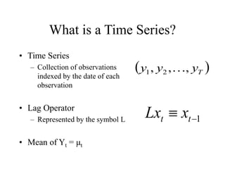
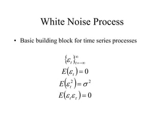
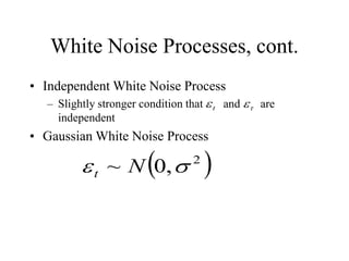
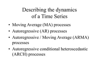
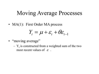
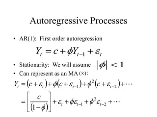
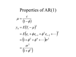
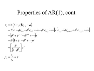
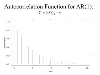
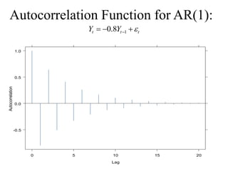
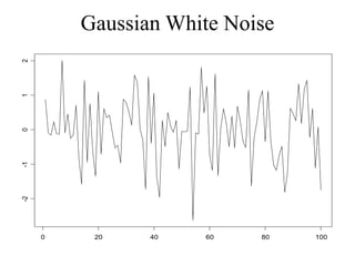
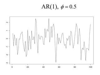
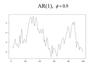
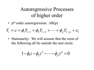
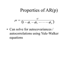
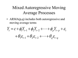
This document provides an introduction to time series analysis. It defines key concepts such as time series, lag operators, mean, autocovariance, stationarity, white noise processes, moving average processes, autoregressive processes, and mixed autoregressive moving average processes. Examples are provided to illustrate properties of different time series models including their autocorrelation functions.

1. An Introduction to Time Series
Ginger Davis
VIGRE Computational Finance Seminar
Rice University
November 26, 2003

2. What is a Time Series?
• Time Series
– Collection of observations
indexed by the date of each
observation
• Lag Operator
– Represented by the symbol L
• Mean of Yt = μt
 
T
y
y
y ,
,
, 2
1 
1

 t
t x
Lx

3. White Noise Process
• Basic building block for time series processes
 
 
 
  0
0
2
2













t
t
t
t
t
E
E
E

4. White Noise Processes, cont.
• Independent White Noise Process
– Slightly stronger condition that and are
independent
• Gaussian White Noise Process
 
2
,
0
~ 
 N
t
t
 


5. Autocovariance
• Covariance of Yt with its own lagged value
• Example: Calculate autocovariances for:
  
j
t
j
t
t
t
jt Y
Y
E 
 

 


    
j
t
t
j
t
t
jt
t
t
E
Y
Y
E
Y

 













6. Stationarity
• Covariance-stationary or weakly stationary
process
– Neither the mean nor the autocovariances depend on
the date t
 
   j
j
t
t
t
Y
Y
E
Y
E










7. Stationarity, cont.
• 2 processes
– 1 covariance stationary, 1 not covariance
stationary
t
t
t
t
t
Y
Y









8. Stationarity, cont.
• Covariance stationary processes
– Covariance between Yt and Yt-j depends only on
j (length of time separating the observations) and
not on t (date of the observation)
j
j 
 


9. Stationarity, cont.
• Strict stationarity
– For any values of j1, j2, …, jn, the joint
distribution of (Yt, Yt+j1
, Yt+j2
, ..., Yt+jn
) depends
only on the intervals separating the dates and
not on the date itself

10. Gaussian Processes
• Gaussian process {Yt}
– Joint density
is Gaussian for any
• What can be said about a covariance stationary
Gaussian process?
 
n
n
j
t
j
t j
t
j
t
t
Y
Y
Y y
y
y
f 



,
,
, 1
1
1 ,
,
, 

n
j
j
j ,
,
, 2
1 

11. Ergodicity
• A covariance-stationary process is said to be
ergodic for the mean if
converges in probability to E(Yt) as



T
t
t
y
T
y
1
1


T

12. Describing the dynamics
of a Time Series
• Moving Average (MA) processes
• Autoregressive (AR) processes
• Autoregressive / Moving Average (ARMA)
processes
• Autoregressive conditional heteroscedastic
(ARCH) processes

13. Moving Average Processes
• MA(1): First Order MA process
• “moving average”
– Yt is constructed from a weighted sum of the two
most recent values of .
1



 t
t
t
Y 




14. Properties of MA(1)
 
   
 
 
     
 
   0
1
2
2
2
1
2
2
2
1
1
2
1
1
1
2
2
2
1
2
1
2
2
1
2































































j
t
t
t
t
t
t
t
t
t
t
t
t
t
t
t
t
t
t
t
t
t
t
t
Y
Y
E
E
E
Y
Y
E
E
E
Y
E
Y
E
for j>1

15. MA(1)
• Covariance stationary
– Mean and autocovariances are not functions of time
• Autocorrelation of a covariance-stationary
process
• MA(1)
0


 j
j 
   
2
2
2
2
1
1
1 










16. Autocorrelation Function for White Noise:
0.0
0.2
0.4
0.6
0.8
1.0
0 5 10 15 20
Lag
Autocorrelation
t
t
Y 


17. Autocorrelation Function for MA(1):
1
8
.
0 

 t
t
t
Y 

0.0
0.2
0.4
0.6
0.8
1.0
0 5 10 15 20
Lag
Autocorrelation

18. Moving Average Processes
of higher order
• MA(q): qth order moving average process
• Properties of MA(q)
q
t
q
t
t
t
t
Y 

 




 






 
2
2
1
1
 
 
q
j
q
j
j
j
q
q
j
j
j
j
q
















,
0
,
,
2
,
1
,
1
2
2
2
1
1
2
2
2
2
2
1
0



















19. Autoregressive Processes
• AR(1): First order autoregression
• Stationarity: We will assume
• Can represent as an MA
t
t
t Y
c
Y 
 

 1
1


     
 

























2
2
1
2
2
1
1
t
t
t
t
t
t
t
c
c
c
c
Y










:
)
(

20. Properties of AR(1)
 
 
 
 
 
2
2
2
4
2
2
2
2
1
2
0
1
1
1































t
t
t
t
E
Y
E
c

21. Properties of AR(1), cont.
  
   
 
 
 
j
j
j
j
j
j
j
j
j
t
j
t
j
t
j
t
j
t
t
t
j
t
t
j
E
Y
Y
E






































































0
2
2
2
4
2
2
4
2
2
2
1
2
2
1
1
1 





22. Autocorrelation Function for AR(1):
t
t
t Y
Y 

 1
8
.
0
0.0
0.2
0.4
0.6
0.8
1.0
0 5 10 15 20
Lag
Autocorrelation

23. Autocorrelation Function for AR(1):
t
t
t Y
Y 


 1
8
.
0
-0.5
0.0
0.5
1.0
0 5 10 15 20
Lag
Autocorrelation

24. Gaussian White Noise
0 20 40 60 80 100
-2
-1
0
1
2

25. AR(1),
0 20 40 60 80 100
-3
-2
-1
0
1
2 5
.
0



26. AR(1),
0 20 40 60 80 100
-2
0
2
4 9
.
0



27. AR(1),
0 20 40 60 80 100
-4
-2
0
2
4 9
.
0




28. Autoregressive Processes
of higher order
• pth order autoregression: AR(p)
• Stationarity: We will assume that the roots of
the following all lie outside the unit circle.
t
p
t
p
t
t
t Y
Y
Y
c
Y 


 




 

 
2
2
1
1
0
1 2
2
1 



 p
p z
z
z 

 

29. Properties of AR(p)
• Can solve for autocovariances /
autocorrelations using Yule-Walker
equations
 
p
c










2
1
1

30. Mixed Autoregressive Moving
Average Processes
• ARMA(p,q) includes both autoregressive and
moving average terms
q
t
q
t
t
t
p
t
p
t
t
t Y
Y
Y
c
Y




























2
2
1
1
2
2
1
1

31. Time Series Models
for Financial Data
• A Motivating Example
– Federal Funds rate
– We are interested in forecasting not only the
level of the series, but also its variance.
– Variance is not constant over time

32. U. S. Federal Funds Rate
Time
1955 1960 1965 1970 1975
2
4
6
8
10
12

33. Modeling the Variance
• AR(p):
• ARCH(m)
– Autoregressive conditional heteroscedastic process
of order m
– Square of ut follows an AR(m) process
– wt is a new white noise process
t
p
t
p
t
t
t u
y
y
y
c
y 




 

 

 
2
2
1
1
t
m
t
m
t
t
t w
u
u
u
u 




 


2
2
2
2
2
1
1
2



 

34. References
• Investopia.com
• Economagic.com
• Hamilton, J. D. (1994), Time Series
Analysis, Princeton, New Jersey: Princeton
University Press.