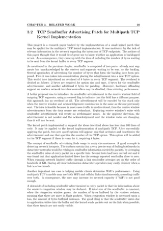
1) The document describes a TCP traffic monitoring and debugging tool created as a bachelor's thesis project. The tool aims to help cloud providers better understand application needs by determining metrics and statistics of TCP connections.
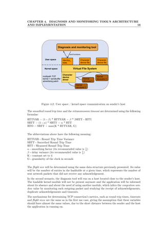
2) Key aspects of the tool include inferring important TCP connection variables like congestion window, combining these with socket-level traffic logs, and a Linux kernel module. Sendbuffer advertising is used to test the tool's accuracy in detecting application-limited connections.
3) The tool seeks to identify network problems by monitoring TCP connections and determining the limiting factor (bandwidth, latency etc.). It displays statistics like RTT, retransmissions and other counters to help cloud operators optimize traffic.


![CHAPTER 5. TESTING 26
As one can see, the physical machines we had access to were used as a mini-network. First, the
multipath TCP kernel sources was copied on the cluster’s filesystem. After that, the sendbuffer
advertising kernel patch was applied to these sources. A configuration file for the multipath
TCP kernel was created, then it was recompiled. The compilation was a success, and after en-
abling the sendbuffer advertising option, a new TCP option emerged when capturing outgoing
network packets using tcpdump tool.
1 18:50:49.583088 IP 10.0.1.1.59832 > 10.0.2.1.12345: Flags [.], seq
36024:37464, ack 1, win 229, options [nop,nop,TS val 4294832922
ecr 717377,nop,nop,unknown-211 0x00005fa0], length 1440
Listing 5.1: Example of tcpdump capture
The next step was configuring the computer acting as a router as a default gateway for the
computer acting as a sender. The same actions were considered for the computer acting as a
receiver, which was the default gateway for the router. On the computer placed in the middle of
the improvised network ip forwarding had to be enabled. For achieving this goal a configuration
script that assigns an IP address and default gateway to each network interface of this machine
was written.
1 #!/bin/bash
2
3 ifconfig eth13 up
4 ip a a 10.0.1.2/24 dev eth13
5 route add default gw 10.0.1.1 eth13
6
7 ifconfig eth10 up
8 ip a a 10.0.2.2/24 dev eth10
9 route add default gw 10.0.2.1 eth10
10
11 echo "1" > /proc/sys/net/ipv4/ip_forward
Listing 5.2: Configuration script for Computer9
Both links in this mini-network had 1 Gbps bandwidth. To simulate different situations, includ-
ing variance in detection point’s placement, dummynet tool was used for varying the bandwidth
and delay of TCP traffic on a specified network interface. Dummynet is an application that
simulates bandwidth limitations, packet losses, or delays, but also multipath effects. It may
be used both on the machine running the user’s application, or on external devices acting as
switches or routers.
1 insmod ipfw_mod.ko
2 ipfw add pipe 1 ip from any to any in via eth13
3 ipfw pipe 1 config bw 200Mbps delay 10ms
Listing 5.3: Example of dummynet tool usage on computer9](https://image.slidesharecdn.com/189311cd-acc5-47df-ba09-0f1ae7057a92-150923082807-lva1-app6892/85/thesis-32-320.jpg)

![Bibliography
[1] W. Richard Stevens, Kevin R. Fall, TCP/IP Illustrated vol. 1
[2] Joao Taveira Araujo, Raul Landa, Richard G. Clegg, George Pavlou, Kensuke Fukuda, A
longitudinal analysis of Internet rate limitations.
[3] Injong Rhee, and Lisong Xu, CUBIC: A New TCP-Friendly High-Speed TCP Variant.
[4] Alexandru Agache, Costin Raiciu, Oh Flow, Are Thou Happy? TCP sendbuffer advertising
for make benefit of clouds and tenants.
[5] RINC Architecture, Mojgan Ghashemi, Theophilus Benson, Jennifer Rexford, RINC: Real-
Time Inference-based Network Diagnosis in the Cloud.
[6] Sharad Jaiswal, Gianluca Iannaccone, Christophe Diot, Jim Kurose, Don Towsley, Inferring
TCP Connection Characteristics Through Passive Measurements.
[7] D.J.Leith, R.N.Shorten, G.McCullagh, Experimental evaluation of Cubic-TCP.
[8] M. Yu, A. Greenberg, D. Maltz, J. Rexford, L. Yuan, S. Kandula, and C. Kim. Profiling
network performance for multi-tier data center applications, 2011.
[9] M. Allman, V. Paxson, Request for Comments: 5681, Sep. 2009.
[10] K. Claffy, Greg Miller, and Kevin Thompson. The Nature of the Beast: Recent Traffic
Measurements from an Internet Backbone. In Proceedings of INET, 1998.
[11] Chuck Fraleigh and et. al. Packet-Level Traffic Measurements from a Tier-1 IP Backbone.
ATL Technical Report TR01-ATL-110101, Sprint, Nov. 2001.
[12] Sean McCreary and Kc Claffy. Trends in Wide Area IP Traffic Patterns: A View from Ames
Internet Exchange. In Proceedings of the 13th ITC Specialist Seminar on Measurement and
Modeling of IP Traffic, Monterey, CA, Jan. 2000.
34](https://image.slidesharecdn.com/189311cd-acc5-47df-ba09-0f1ae7057a92-150923082807-lva1-app6892/85/thesis-40-320.jpg)