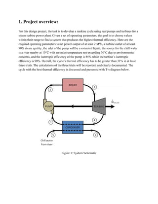
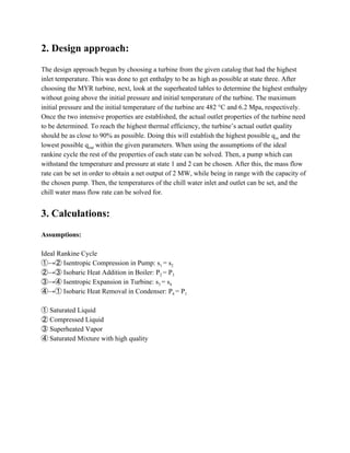
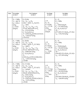
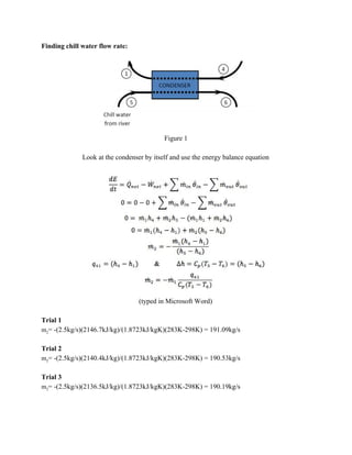
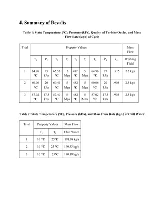
MAE 204
Final Project
Group Members:
Keshshoth Kanagalingam (Sec-B)
Ian Salathiel (Sec-B)
Peter Flood (Sec-F)
Richard Stacey (Sec-B)
Table of Contents
1. Project Overview ………………………………………………………….. X
2. Design Approach ………………………………………………………….. X
3. Calculations …………………………………………………………….…. X
4. Summary of Results……………………………………………………….. X
5. T-s Diagram………………………………………………………………... X
6. Discussions ………………………………………………………………... X
7. Conclusions………………………………………………………………... X
1. Project overview:
For this design project, the task is to develop a rankine cycle using real pumps and turbines for a
steam turbine power plant. Given a set of operating parameters, the goal is to choose values
within their range to find a system that produces the highest thermal efficiency. Here are the
required operating parameters: a net power output of at least 2 MW, a turbine outlet of at least
90% steam quality, the inlet of the pump will be a saturated liquid, the source for the chill water
is a river nearby at 10°C with an outlet temperature not exceeding 30°C due to environmental
concerns, and the isentropic efficiency of the pump is 85% while the turbine’s isentropic
efficiency is 90%. Overall, the cycle’s thermal efficiency has to be greater than 31% in at least
three trials. The calculations of the three trials will be recorded and clearly documented. The
cycle with the best thermal efficiency is discussed and presented with T-s diagram below.
Figure 1: System Schematic
2. Design approach:
The design approach begun by choosing a turbine from the given catalog that had the highest
inlet temperature. This was done to get enthalpy to be as high as possible at state three. After
choosing the MYR turbine, next, look at the superheated tables to determine the highest enthalpy
without going above the initial pressure and initial temperature of the turbine. The maximum
initial pressure and the initial temperature of the turbine are 482 °C and 6.2 Mpa, respectively.
Once the two intensive properties are established, the actual outlet properties of the turbine need
to be determined. To reach the highest thermal efficiency, the turbine’s actual outlet quality
should be as close to 90% as possible. Doing this will establish the highest possible q​in​ and the
lowest possible q​out​ within the given parameters. When using the assumptions of the ideal
rankine cycle the rest of the properties of each state can be solved. Then, a pump which can
withstand the temperature and pressure at state 1 and 2 can be chosen. After this, the mass flow
rate can be set in order to obtain a net output of 2 MW, while being in range with the capacity of
the chosen pump. Then, the temperatures of the chill water inlet and outlet can be set, and the
chill water mass flow rate can be solved for.
3. Calculations:
Assumptions:
Ideal Rankine Cycle
①→② Isentropic Compression in Pump: ​s​1 ​= s​2
②→③ Isobaric Heat Addition in Boiler: ​P​2 ​= P​3
③→④ Isentropic Expansion in Turbine: ​s​3 ​= s​4
④→① Isobaric Heat Removal in Condenser: ​P​4 ​= P​1
① Saturated Liquid
② Compressed Liquid
③ Superheated Vapor
④ Saturated Mixture with high quality
Trial For turbine
@ state 3
For Condenser
@ state 4
For Pump
@ state 1
For Boiler
@ state 2
1 P​3​ = 5 MPa
T​3​ = 482 ​°C
h​3​= 3392.4
kJ/kg
s​3​= 6.922
kJ/kg*k
P​4​=25 kPa
S​s4​ = S​f4​ + x​4s​*S​fg
6.922 = .8932 +x ​4s​*(6.937)
x​4s​ =.8691
h​4s​ = h​f4​ + x​4s​ * h​fg4​ => h​4s
271.96+.8691(2345.5)=h​4s
h​4s​ =2310.43 kJ/kg
n​t​ = (h​3​-h​4​)/(h​3​-h​4s​)
.9 = (3392.4-h​4a​)/(3392.4-2310.43)
h​4a​ = 2418.627 kJ/kg
x=0.91523
x=0
P​4​ = P​1
P​1​=25 kpa
h​1​ = 271.96
kJ/kg
s​1​ = .8932
kJ/kg*k
P​2​ = P​3
P​2​= 5 MPa
s​1​=s​2s
s​2s​ =.8932 kJ/kg*k
h​2s​ = 277.4955 kJ/kg
n​t​ = (h​2s​-h​1​)/(h​2​-h​1​)=
.85 =
(277.4955-271.96)/(h​2a​-271.96)=
h​2a​ = 278.4724 kJ/kg
2 P​3​ = 5 MPa
T​3​ = 482 ​°C
h​3​= 3392.4
kJ/kg
s​3​= 6.922
kJ/kg*k
P​4​=20 kPa
S​s4​ = S​f4​ + x​4s​*S​fg
6.922 = .8320 +x ​4s​*(7.7052)
x​4s​ =.86075
h​4s​ = h​f4​ + x​4s​ * h​fg4​ => h​4s
251.42+.86075(2357.5)=h​4s
h​4s​ =2280.6381 kJ/kg
n​t​ = (h​3​-h​4​)/(h​3​-h​4s​)
.9 =
(3392.4-h​4a​)/(3392.4-2280.6381)
h​4a​ = 2391.8143 kJ/kg
x=0.908
x=0
P​4​ = P​1
P​1​=20 kpa
h​1​ = 251.42
kJ/kg
s​1​ = .8320
kJ/kg*k
P​2​ = P​3
P​2​= 5 MPa
s​1​=s​2s
s​2s​ =.8320 kJ/kg*k
h​2s​ = 256.4925 kJ/kg
n​t​ = (h​2s​-h​1​)/(h​2​-h​1​)=
.85 =
(256.4925-251.42)/(h​2a​-251.42)=
h​2a​ = 257.3876 kJ/kg
3 P​3​ = 5 MPa
T​3​ = 482 ​°C
h​3​= 3392.4
kJ/kg
s​3​= 6.922
kJ/kg*k
P​4​=17.5 kPa
S​4s​ = S​f4​ + x​4s​*S​fg
6.922 = .7934 +x ​4s​*(7.1637)
x​4s​ =.855647
h​4s​ = h​f4​ + x​4s​ * h​fg4​ => h​4s
238.68+.855647(2364.9)=h​4s
h​4s​ =2262.2 kJ/kg
n​t​ = (h​3​-h​4​)/(h​3​-h​4s​)
.9 = (3392.4-h​4a​)/(3392.4-2262.2)
h​4a​ = 2375.22 kJ/kg
x=0.903
x=0
P​4​ = P​1
P​1​=17.5 kpa
h​1​ = 238.68
kJ/kg
s​1​ = .7934
kJ/kg
P​2​ = P​3
P​2​= 5 MPa
s​1​=s​2s
s​2s​ =.7934 kJ/kg*k
h​2s​ = 243.9565 kJ/kg
n​t​ = (h​2s​-h​1​)/(h​2​-h​1​)=
.85 =
(243.9565-238.68)/(h​2a​-238.68)=
h​2a​ = 244.8876 kJ/kg
Finding chill water flow rate:
Figure 1
Look at the condenser by itself and use the energy balance equation
(typed in Microsoft Word)
Trial 1
m​2​= -(2.5kg/s)(2146.7kJ/kg)/(1.8723kJ/kgK)(283K-298K) = 191.09kg/s
Trial 2
m​2​= -(2.5kg/s)(2140.4kJ/kg)/(1.8723kJ/kgK)(283K-298K) = 190.53kg/s
Trial 3
m​2​= -(2.5kg/s)(2136.5kJ/kg)/(1.8723kJ/kgK)(283K-298K) = 190.19kg/s
4. Summary of Results
Table 1: State Temperature (°C), Pressure (kPa), Quality of Turbine Outlet, and Mass
Flow Rate (kg/s) of Cycle
Trial Property Values Mass
Flow
T​1 P​1 T​2 P​2 T​3 P​3 T​4 P​4 x​4 Working
Fluid
1 64.96
°C
25
kPa
65.53
°C
5
Mpa
482
°C
5
Mpa
64.96
​°C
25
kPa
.915 2.5 kg/s
2 60.06
​°C
20
kPa
60.49
°C
5
Mpa
482
°C
5
Mpa
60.06
°C
20
kPa
.908 2.5 kg/s
3 57.02
°C
17.5
kPa
57.49
°C
5
Mpa
482
°C
5
MPa
57.02
°C
17.5
kPa
.903 2.5 kg/s
Table 2: State Temperature (°C), Pressure (kPa), and Mass Flow Rate (kg/s) of Chill Water
Trial Property Values Mass Flow
T​5 T​6 ​Chill Water
1 10 ​°C 25​°C 191.09 kg/s
2 10 ​°C 25 ​°C 190.53 kg/s
3 10 ​°C 25​°C 190.19 kg/s
Table 3: Computed Heat (kJ/kg), Work (kJ/kg), Net Power (kW) and Thermal Efficiency
Trial q​12
(kJ
/kg
)
w​12
(kJ/kg)
q​23
(kJ/kg)
w​23
(kJ/
kg)
q​34
(kJ/
kg)
w​34
(kJ/kg)
q​41
(kJ/kg)
w​41
(kJ/
kg)
Net Power
(kW)
Thermal
Efficiency
1 0 6.5124 3113.9 0 0 973.77 2146.7 0 2418.2 31.06%
2 0 5.9676 3135.0 0 0 1000.6 2140.4 0 2486.5 31.73%
3 0 6.2076 3147.5 0 0 1017.2 2136.5 0 2527.4 32.12%
5. T-s Diagrams:
State 1 State 2 State 3 State 4
T=57.02 °C T=57.488 °C T=482 °C T=57.02 °C
P=17.5 kPa P=5 Mpa P=5 MPa P=17.5 kPa
6. Discussion:
The most important parameters in this design are the temperature and pressure at the inlet of the
turbine, and the pressure and temperature at the outlet of the turbine. In this process, the turbine
with the highest inlet temperature and pressure was considered in order to maximize enthalpy at
state three which will increase the heat in. Next, the main objective was to find the lowest
pressure and temperature at the outlet to minimize the enthalpy at state four while still
maintaining a quality of 90%.This was the main challenge of the design approach. After the first
successful trial with 25 kPa for the outlet turbine pressure, the inlet turbine pressure and
temperature were kept constant while decreasing the outlet pressure to the lowest pressure so that
the turbine will still produce a steam quality of 90%. The pressure was 17.5 kPa, which produced
a quality of 90.03%. A quality of 90.03% is extremely close to 90%. As a result, the temperature
and pressure of the turbine inlet were kept constant for each trial while changing the outlet
temperature and pressure. Once the turbine inlet temperature and pressure were set, the most
important parameters that affected the efficiency was the outlet temperature and pressure. After
the pressure and temperature were chosen at the inlet and outlet of the turbine, the pressure and
temperature at the inlet and outlet of the pump can be solved for by an analysis of the rankine
cycle. These states have to fall within the parameters of a given pump. Although these states fell
within the range of all given pumps, pump MHB was chosen because it has the largest capacity.
The mass flow rate of the cycle was then set to 2.5 kg/s in order to obtain a net output of 2 MW
for each trial. Then, temperatures for the chill water inlet and outlet were chosen within the
specified range, and then the chill water mass flow rate was solved for.
7. Conclusion:
Throughout the design process many unexpected factors and problems were encountered which
constantly changed the approach to engineer a steam turbine plant that satisfied the given
parameters. All three designs achieved the goal of reaching a thermal efficiency above 31%.
After taking everything into consideration, the process was narrowed down to manipulating the
temperatures and pressures at the inlet and outlet states of the turbine, ultimately affecting the
thermal efficiency. However, a lot of different factors were still not taken into consideration. The
cycle running at very high temperatures and pressures to achieve a high efficiency could cause
parts to diminish and fail overtime or limit how long the system can run until damage occurs.
The various advantages and disadvantages of materials and the costs of replacements need to be
taken into consideration in a non-ideal situation. This portrays how complex and challenging the
design of a high efficiency steam turbine power plant is.

Thermo Final Project

  • 1.
    MAE 204 Final Project GroupMembers: Keshshoth Kanagalingam (Sec-B) Ian Salathiel (Sec-B) Peter Flood (Sec-F) Richard Stacey (Sec-B)
  • 2.
    Table of Contents 1.Project Overview ………………………………………………………….. X 2. Design Approach ………………………………………………………….. X 3. Calculations …………………………………………………………….…. X 4. Summary of Results……………………………………………………….. X 5. T-s Diagram………………………………………………………………... X 6. Discussions ………………………………………………………………... X 7. Conclusions………………………………………………………………... X
  • 3.
    1. Project overview: Forthis design project, the task is to develop a rankine cycle using real pumps and turbines for a steam turbine power plant. Given a set of operating parameters, the goal is to choose values within their range to find a system that produces the highest thermal efficiency. Here are the required operating parameters: a net power output of at least 2 MW, a turbine outlet of at least 90% steam quality, the inlet of the pump will be a saturated liquid, the source for the chill water is a river nearby at 10°C with an outlet temperature not exceeding 30°C due to environmental concerns, and the isentropic efficiency of the pump is 85% while the turbine’s isentropic efficiency is 90%. Overall, the cycle’s thermal efficiency has to be greater than 31% in at least three trials. The calculations of the three trials will be recorded and clearly documented. The cycle with the best thermal efficiency is discussed and presented with T-s diagram below. Figure 1: System Schematic
  • 4.
    2. Design approach: Thedesign approach begun by choosing a turbine from the given catalog that had the highest inlet temperature. This was done to get enthalpy to be as high as possible at state three. After choosing the MYR turbine, next, look at the superheated tables to determine the highest enthalpy without going above the initial pressure and initial temperature of the turbine. The maximum initial pressure and the initial temperature of the turbine are 482 °C and 6.2 Mpa, respectively. Once the two intensive properties are established, the actual outlet properties of the turbine need to be determined. To reach the highest thermal efficiency, the turbine’s actual outlet quality should be as close to 90% as possible. Doing this will establish the highest possible q​in​ and the lowest possible q​out​ within the given parameters. When using the assumptions of the ideal rankine cycle the rest of the properties of each state can be solved. Then, a pump which can withstand the temperature and pressure at state 1 and 2 can be chosen. After this, the mass flow rate can be set in order to obtain a net output of 2 MW, while being in range with the capacity of the chosen pump. Then, the temperatures of the chill water inlet and outlet can be set, and the chill water mass flow rate can be solved for. 3. Calculations: Assumptions: Ideal Rankine Cycle ①→② Isentropic Compression in Pump: ​s​1 ​= s​2 ②→③ Isobaric Heat Addition in Boiler: ​P​2 ​= P​3 ③→④ Isentropic Expansion in Turbine: ​s​3 ​= s​4 ④→① Isobaric Heat Removal in Condenser: ​P​4 ​= P​1 ① Saturated Liquid ② Compressed Liquid ③ Superheated Vapor ④ Saturated Mixture with high quality
  • 5.
    Trial For turbine @state 3 For Condenser @ state 4 For Pump @ state 1 For Boiler @ state 2 1 P​3​ = 5 MPa T​3​ = 482 ​°C h​3​= 3392.4 kJ/kg s​3​= 6.922 kJ/kg*k P​4​=25 kPa S​s4​ = S​f4​ + x​4s​*S​fg 6.922 = .8932 +x ​4s​*(6.937) x​4s​ =.8691 h​4s​ = h​f4​ + x​4s​ * h​fg4​ => h​4s 271.96+.8691(2345.5)=h​4s h​4s​ =2310.43 kJ/kg n​t​ = (h​3​-h​4​)/(h​3​-h​4s​) .9 = (3392.4-h​4a​)/(3392.4-2310.43) h​4a​ = 2418.627 kJ/kg x=0.91523 x=0 P​4​ = P​1 P​1​=25 kpa h​1​ = 271.96 kJ/kg s​1​ = .8932 kJ/kg*k P​2​ = P​3 P​2​= 5 MPa s​1​=s​2s s​2s​ =.8932 kJ/kg*k h​2s​ = 277.4955 kJ/kg n​t​ = (h​2s​-h​1​)/(h​2​-h​1​)= .85 = (277.4955-271.96)/(h​2a​-271.96)= h​2a​ = 278.4724 kJ/kg 2 P​3​ = 5 MPa T​3​ = 482 ​°C h​3​= 3392.4 kJ/kg s​3​= 6.922 kJ/kg*k P​4​=20 kPa S​s4​ = S​f4​ + x​4s​*S​fg 6.922 = .8320 +x ​4s​*(7.7052) x​4s​ =.86075 h​4s​ = h​f4​ + x​4s​ * h​fg4​ => h​4s 251.42+.86075(2357.5)=h​4s h​4s​ =2280.6381 kJ/kg n​t​ = (h​3​-h​4​)/(h​3​-h​4s​) .9 = (3392.4-h​4a​)/(3392.4-2280.6381) h​4a​ = 2391.8143 kJ/kg x=0.908 x=0 P​4​ = P​1 P​1​=20 kpa h​1​ = 251.42 kJ/kg s​1​ = .8320 kJ/kg*k P​2​ = P​3 P​2​= 5 MPa s​1​=s​2s s​2s​ =.8320 kJ/kg*k h​2s​ = 256.4925 kJ/kg n​t​ = (h​2s​-h​1​)/(h​2​-h​1​)= .85 = (256.4925-251.42)/(h​2a​-251.42)= h​2a​ = 257.3876 kJ/kg 3 P​3​ = 5 MPa T​3​ = 482 ​°C h​3​= 3392.4 kJ/kg s​3​= 6.922 kJ/kg*k P​4​=17.5 kPa S​4s​ = S​f4​ + x​4s​*S​fg 6.922 = .7934 +x ​4s​*(7.1637) x​4s​ =.855647 h​4s​ = h​f4​ + x​4s​ * h​fg4​ => h​4s 238.68+.855647(2364.9)=h​4s h​4s​ =2262.2 kJ/kg n​t​ = (h​3​-h​4​)/(h​3​-h​4s​) .9 = (3392.4-h​4a​)/(3392.4-2262.2) h​4a​ = 2375.22 kJ/kg x=0.903 x=0 P​4​ = P​1 P​1​=17.5 kpa h​1​ = 238.68 kJ/kg s​1​ = .7934 kJ/kg P​2​ = P​3 P​2​= 5 MPa s​1​=s​2s s​2s​ =.7934 kJ/kg*k h​2s​ = 243.9565 kJ/kg n​t​ = (h​2s​-h​1​)/(h​2​-h​1​)= .85 = (243.9565-238.68)/(h​2a​-238.68)= h​2a​ = 244.8876 kJ/kg
  • 6.
    Finding chill waterflow rate: Figure 1 Look at the condenser by itself and use the energy balance equation (typed in Microsoft Word) Trial 1 m​2​= -(2.5kg/s)(2146.7kJ/kg)/(1.8723kJ/kgK)(283K-298K) = 191.09kg/s Trial 2 m​2​= -(2.5kg/s)(2140.4kJ/kg)/(1.8723kJ/kgK)(283K-298K) = 190.53kg/s Trial 3 m​2​= -(2.5kg/s)(2136.5kJ/kg)/(1.8723kJ/kgK)(283K-298K) = 190.19kg/s
  • 7.
    4. Summary ofResults Table 1: State Temperature (°C), Pressure (kPa), Quality of Turbine Outlet, and Mass Flow Rate (kg/s) of Cycle Trial Property Values Mass Flow T​1 P​1 T​2 P​2 T​3 P​3 T​4 P​4 x​4 Working Fluid 1 64.96 °C 25 kPa 65.53 °C 5 Mpa 482 °C 5 Mpa 64.96 ​°C 25 kPa .915 2.5 kg/s 2 60.06 ​°C 20 kPa 60.49 °C 5 Mpa 482 °C 5 Mpa 60.06 °C 20 kPa .908 2.5 kg/s 3 57.02 °C 17.5 kPa 57.49 °C 5 Mpa 482 °C 5 MPa 57.02 °C 17.5 kPa .903 2.5 kg/s Table 2: State Temperature (°C), Pressure (kPa), and Mass Flow Rate (kg/s) of Chill Water Trial Property Values Mass Flow T​5 T​6 ​Chill Water 1 10 ​°C 25​°C 191.09 kg/s 2 10 ​°C 25 ​°C 190.53 kg/s 3 10 ​°C 25​°C 190.19 kg/s
  • 8.
    Table 3: ComputedHeat (kJ/kg), Work (kJ/kg), Net Power (kW) and Thermal Efficiency Trial q​12 (kJ /kg ) w​12 (kJ/kg) q​23 (kJ/kg) w​23 (kJ/ kg) q​34 (kJ/ kg) w​34 (kJ/kg) q​41 (kJ/kg) w​41 (kJ/ kg) Net Power (kW) Thermal Efficiency 1 0 6.5124 3113.9 0 0 973.77 2146.7 0 2418.2 31.06% 2 0 5.9676 3135.0 0 0 1000.6 2140.4 0 2486.5 31.73% 3 0 6.2076 3147.5 0 0 1017.2 2136.5 0 2527.4 32.12% 5. T-s Diagrams: State 1 State 2 State 3 State 4 T=57.02 °C T=57.488 °C T=482 °C T=57.02 °C P=17.5 kPa P=5 Mpa P=5 MPa P=17.5 kPa
  • 9.
    6. Discussion: The mostimportant parameters in this design are the temperature and pressure at the inlet of the turbine, and the pressure and temperature at the outlet of the turbine. In this process, the turbine with the highest inlet temperature and pressure was considered in order to maximize enthalpy at state three which will increase the heat in. Next, the main objective was to find the lowest pressure and temperature at the outlet to minimize the enthalpy at state four while still maintaining a quality of 90%.This was the main challenge of the design approach. After the first successful trial with 25 kPa for the outlet turbine pressure, the inlet turbine pressure and temperature were kept constant while decreasing the outlet pressure to the lowest pressure so that the turbine will still produce a steam quality of 90%. The pressure was 17.5 kPa, which produced a quality of 90.03%. A quality of 90.03% is extremely close to 90%. As a result, the temperature and pressure of the turbine inlet were kept constant for each trial while changing the outlet temperature and pressure. Once the turbine inlet temperature and pressure were set, the most important parameters that affected the efficiency was the outlet temperature and pressure. After the pressure and temperature were chosen at the inlet and outlet of the turbine, the pressure and temperature at the inlet and outlet of the pump can be solved for by an analysis of the rankine cycle. These states have to fall within the parameters of a given pump. Although these states fell within the range of all given pumps, pump MHB was chosen because it has the largest capacity. The mass flow rate of the cycle was then set to 2.5 kg/s in order to obtain a net output of 2 MW for each trial. Then, temperatures for the chill water inlet and outlet were chosen within the specified range, and then the chill water mass flow rate was solved for. 7. Conclusion: Throughout the design process many unexpected factors and problems were encountered which constantly changed the approach to engineer a steam turbine plant that satisfied the given parameters. All three designs achieved the goal of reaching a thermal efficiency above 31%. After taking everything into consideration, the process was narrowed down to manipulating the temperatures and pressures at the inlet and outlet states of the turbine, ultimately affecting the thermal efficiency. However, a lot of different factors were still not taken into consideration. The cycle running at very high temperatures and pressures to achieve a high efficiency could cause parts to diminish and fail overtime or limit how long the system can run until damage occurs. The various advantages and disadvantages of materials and the costs of replacements need to be taken into consideration in a non-ideal situation. This portrays how complex and challenging the design of a high efficiency steam turbine power plant is.