Download free for 30 days
Sign in
Upload
Language (EN)
Support
Business
Mobile
Social Media
Marketing
Technology
Art & Photos
Career
Design
Education
Presentations & Public Speaking
Government & Nonprofit
Healthcare
Internet
Law
Leadership & Management
Automotive
Engineering
Software
Recruiting & HR
Retail
Sales
Services
Science
Small Business & Entrepreneurship
Food
Environment
Economy & Finance
Data & Analytics
Investor Relations
Sports
Spiritual
News & Politics
Travel
Self Improvement
Real Estate
Entertainment & Humor
Health & Medicine
Devices & Hardware
Lifestyle
Change Language
Language
English
Español
Português
Français
Deutsche
Cancel
Save
EN
Uploaded by
Ruo Ando
321 views
TensorflowとKerasによる深層学習のプログラム実装実践講座
TensorflowとKerasによる深層学習のプログラム実装実践講座 2018年11月14日(水) 10:30-17:30
Engineering
◦
Read more
1
Save
Share
Embed
Embed presentation
Download
Download to read offline
1
/ 44
2
/ 44
3
/ 44
4
/ 44
5
/ 44
6
/ 44
7
/ 44
8
/ 44
9
/ 44
10
/ 44
11
/ 44
12
/ 44
13
/ 44
14
/ 44
15
/ 44
16
/ 44
17
/ 44
18
/ 44
19
/ 44
20
/ 44
21
/ 44
22
/ 44
23
/ 44
24
/ 44
25
/ 44
26
/ 44
27
/ 44
28
/ 44
29
/ 44
30
/ 44
31
/ 44
32
/ 44
33
/ 44
34
/ 44
35
/ 44
36
/ 44
37
/ 44
38
/ 44
39
/ 44
40
/ 44
41
/ 44
42
/ 44
43
/ 44
44
/ 44
More Related Content
PPT
ΝΙΚΟΣ ΚΑΖΑΝΤΖΑΚΗΣ
by
ELENI EFSTATHIADOU
PPT
"Ελεύθεροι πολιορκημένοι" ( Οι στοχασμοί)
by
Flora Kyprianou
DOCX
Eγκλίσεις, χρόνοι και η σημασία τους, αύξηση
by
Georgia Dimitropoulou
PDF
[第2版]Python機械学習プログラミング 第16章
by
Haruki Eguchi
PDF
Scikit-learn and TensorFlow Chap-14 RNN (v1.1)
by
孝好 飯塚
PPTX
【macOSにも対応】AI入門「第3回:数学が苦手でも作って使えるKerasディープラーニング」
by
fukuoka.ex
PPTX
AI入門「第3回:数学が苦手でも作って使えるKerasディープラーニング」【旧版】※新版あります
by
fukuoka.ex
PDF
[第2版]Python機械学習プログラミング 第13章
by
Haruki Eguchi
ΝΙΚΟΣ ΚΑΖΑΝΤΖΑΚΗΣ
by
ELENI EFSTATHIADOU
"Ελεύθεροι πολιορκημένοι" ( Οι στοχασμοί)
by
Flora Kyprianou
Eγκλίσεις, χρόνοι και η σημασία τους, αύξηση
by
Georgia Dimitropoulou
[第2版]Python機械学習プログラミング 第16章
by
Haruki Eguchi
Scikit-learn and TensorFlow Chap-14 RNN (v1.1)
by
孝好 飯塚
【macOSにも対応】AI入門「第3回:数学が苦手でも作って使えるKerasディープラーニング」
by
fukuoka.ex
AI入門「第3回:数学が苦手でも作って使えるKerasディープラーニング」【旧版】※新版あります
by
fukuoka.ex
[第2版]Python機械学習プログラミング 第13章
by
Haruki Eguchi
Similar to TensorflowとKerasによる深層学習のプログラム実装実践講座
PDF
[第2版]Python機械学習プログラミング 第14章
by
Haruki Eguchi
PDF
深層学習(講談社)のまとめ(1章~2章)
by
okku apot
PDF
ディープニューラルネット入門
by
TanUkkii
PPTX
Machine Learning Fundamentals IEEE
by
Antonio Tejero de Pablos
PPTX
深層学習とTensorFlow入門
by
tak9029
PDF
PythonによるDeep Learningの実装
by
Shinya Akiba
PPTX
機械学習 / Deep Learning 大全 (2) Deep Learning 基礎編
by
Daiyu Hatakeyama
PDF
[DL Hacks] Deterministic Variational Inference for RobustBayesian Neural Netw...
by
Deep Learning JP
PPTX
tfug-kagoshima
by
tak9029
DOCX
深層学習 Day1レポート
by
taishimotoda
PDF
2018年01月27日 Keras/TesorFlowによるディープラーニング事始め
by
aitc_jp
PDF
深層学習と確率プログラミングを融合したEdwardについて
by
ryosuke-kojima
PDF
SGDによるDeepLearningの学習
by
Masashi (Jangsa) Kawaguchi
PPTX
「機械学習とは?」から始める Deep learning実践入門
by
Hideto Masuoka
PDF
Chainerの使い方と自然言語処理への応用
by
Seiya Tokui
PDF
dl-with-python01_handout
by
Shin Asakawa
PPTX
深層学習の基礎と導入
by
Kazuki Motohashi
PDF
TensorFlowによるニューラルネットワーク入門
by
Etsuji Nakai
PDF
東京都市大学 データ解析入門 10 ニューラルネットワークと深層学習 1
by
hirokazutanaka
PDF
「深層学習」勉強会LT資料 "Chainer使ってみた"
by
Ken'ichi Matsui
[第2版]Python機械学習プログラミング 第14章
by
Haruki Eguchi
深層学習(講談社)のまとめ(1章~2章)
by
okku apot
ディープニューラルネット入門
by
TanUkkii
Machine Learning Fundamentals IEEE
by
Antonio Tejero de Pablos
深層学習とTensorFlow入門
by
tak9029
PythonによるDeep Learningの実装
by
Shinya Akiba
機械学習 / Deep Learning 大全 (2) Deep Learning 基礎編
by
Daiyu Hatakeyama
[DL Hacks] Deterministic Variational Inference for RobustBayesian Neural Netw...
by
Deep Learning JP
tfug-kagoshima
by
tak9029
深層学習 Day1レポート
by
taishimotoda
2018年01月27日 Keras/TesorFlowによるディープラーニング事始め
by
aitc_jp
深層学習と確率プログラミングを融合したEdwardについて
by
ryosuke-kojima
SGDによるDeepLearningの学習
by
Masashi (Jangsa) Kawaguchi
「機械学習とは?」から始める Deep learning実践入門
by
Hideto Masuoka
Chainerの使い方と自然言語処理への応用
by
Seiya Tokui
dl-with-python01_handout
by
Shin Asakawa
深層学習の基礎と導入
by
Kazuki Motohashi
TensorFlowによるニューラルネットワーク入門
by
Etsuji Nakai
東京都市大学 データ解析入門 10 ニューラルネットワークと深層学習 1
by
hirokazutanaka
「深層学習」勉強会LT資料 "Chainer使ってみた"
by
Ken'ichi Matsui
More from Ruo Ando
PDF
KISTI-NII Joint Security Workshop 2023.pdf
by
Ruo Ando
PDF
Gartner 「セキュリティ&リスクマネジメントサミット 2019」- 安藤
by
Ruo Ando
PDF
解説#86 決定木 - ss.pdf
by
Ruo Ando
PDF
SaaSアカデミー for バックオフィス アイドルと学ぶDX講座 ~アイドル戦略に見るDXを専門家が徹底解説~
by
Ruo Ando
PDF
解説#83 情報エントロピー
by
Ruo Ando
PDF
解説#82 記号論理学
by
Ruo Ando
PDF
解説#81 ロジスティック回帰
by
Ruo Ando
PDF
解説#74 連結リスト
by
Ruo Ando
PDF
解説#76 福岡正信
by
Ruo Ando
PDF
解説#77 非加算無限
by
Ruo Ando
PDF
解説#1 C言語ポインタとアドレス
by
Ruo Ando
PDF
解説#78 誤差逆伝播
by
Ruo Ando
PDF
解説#73 ハフマン符号
by
Ruo Ando
PDF
【技術解説20】 ミニバッチ確率的勾配降下法
by
Ruo Ando
PDF
【技術解説4】assertion failureとuse after-free
by
Ruo Ando
PDF
ITmedia Security Week 2021 講演資料
by
Ruo Ando
PPTX
ファジングの解説
by
Ruo Ando
PDF
AI(機械学習・深層学習)との協働スキルとOperational AIの事例紹介 @ ビジネス+ITセミナー 2020年11月
by
Ruo Ando
PDF
【AI実装4】TensorFlowのプログラムを読む2 非線形回帰
by
Ruo Ando
PDF
Intel Trusted Computing Group 1st Workshop
by
Ruo Ando
KISTI-NII Joint Security Workshop 2023.pdf
by
Ruo Ando
Gartner 「セキュリティ&リスクマネジメントサミット 2019」- 安藤
by
Ruo Ando
解説#86 決定木 - ss.pdf
by
Ruo Ando
SaaSアカデミー for バックオフィス アイドルと学ぶDX講座 ~アイドル戦略に見るDXを専門家が徹底解説~
by
Ruo Ando
解説#83 情報エントロピー
by
Ruo Ando
解説#82 記号論理学
by
Ruo Ando
解説#81 ロジスティック回帰
by
Ruo Ando
解説#74 連結リスト
by
Ruo Ando
解説#76 福岡正信
by
Ruo Ando
解説#77 非加算無限
by
Ruo Ando
解説#1 C言語ポインタとアドレス
by
Ruo Ando
解説#78 誤差逆伝播
by
Ruo Ando
解説#73 ハフマン符号
by
Ruo Ando
【技術解説20】 ミニバッチ確率的勾配降下法
by
Ruo Ando
【技術解説4】assertion failureとuse after-free
by
Ruo Ando
ITmedia Security Week 2021 講演資料
by
Ruo Ando
ファジングの解説
by
Ruo Ando
AI(機械学習・深層学習)との協働スキルとOperational AIの事例紹介 @ ビジネス+ITセミナー 2020年11月
by
Ruo Ando
【AI実装4】TensorFlowのプログラムを読む2 非線形回帰
by
Ruo Ando
Intel Trusted Computing Group 1st Workshop
by
Ruo Ando
TensorflowとKerasによる深層学習のプログラム実装実践講座
1.
TensorflowとKerasによる 深層学習のプログラム実装実践講座 2018年11月14日(水) 10:30-17:30 国立情報学研究所 安藤類央 WEB公開版
2.
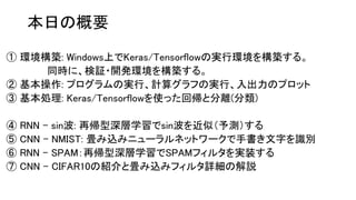
本日の概要 ① 環境構築: Windows上でKeras/Tensorflowの実行環境を構築する。 同時に、検証・開発環境を構築する。 ②
基本操作: プログラムの実行、計算グラフの実行、入出力のプロット ③ 基本処理: Keras/Tensorflowを使った回帰と分離(分類) ④ RNN – sin波: 再帰型深層学習でsin波を近似(予測)する ⑤ CNN – NMIST: 畳み込みニューラルネットワークで手書き文字を識別 ⑥ RNN – SPAM:再帰型深層学習でSPAMフィルタを実装する ⑦ CNN – CIFAR10の紹介と畳み込みフィルタ詳細の解説
3.
①環境構築 1.1 インストールするソフトウェア 1.2 環境構築の手順 1.3
環境構築① Tensorflow 1.4 環境構築② Keras 1.5 構築環境③ GitHub / Atom 1.6 ソフトウェア・ハードウェアスタックの概要
4.
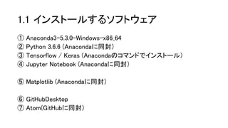
1.1 インストールするソフトウェア ① Anaconda3-5.3.0-Windows-x86_64 ②
Python 3.6.6 (Anacondaに同封) ③ Tensorflow / Keras (Anacondaのコマンドでインストール) ④ Jupyter Notebook (Anacondaに同封) ⑤ Matplotlib (Anacondaに同封) ⑥ GitHubDesktop ⑦ Atom(GitHubに同封)
5.
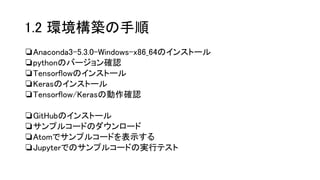
1.2 環境構築の手順 ❏Anaconda3-5.3.0-Windows-x86_64のインストール ❏pythonのバージョン確認 ❏Tensorflowのインストール ❏Kerasのインストール ❏Tensorflow/Kerasの動作確認 ❏GitHubのインストール ❏サンプルコードのダウンロード ❏Atomでサンプルコードを表示する ❏Jupyterでのサンプルコードの実行テスト
6.
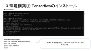
1.3 環境構築① Tensorflowのインストール imort
tensorflow as tf hello = tf.constant(“hello tensorflow”) sess = tf.session() print(sess.run(hello)) exit() 定数に文字列を設定し、セッションを出力することで 出力します。
7.
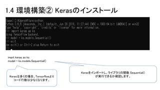
1.4 環境構築② Kerasのインストール imprt
keras as ks model = ks.models.Sequential() Kerasをインポートし、ライブラリの関数 Sequential() が実行できるか確認します。Kerasは多くの場合、Tensorflowより コード行数は少なくなります。
8.
1.5 環境構築③GitHub/Atomでサンプルコードを表示
9.
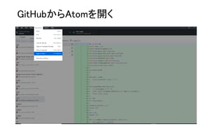
GitHubからAtomを開く
10.
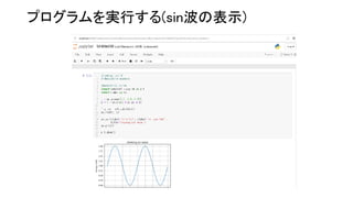
プログラムを実行する(sin波の表示)
11.
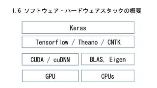
1.6 ソフトウェア・ハードウェアスタックの概要 Keras Tensorflow /
Theano / CNTK CUDA / cuDNN BLAS, Eigen GPU CPUs
12.
②基本操作 2.1 最小の深層学習プログラム 2.2 ランダムプロット 2.3
SIN波のプロット 2.4 計算グラフの構築と実行
13.
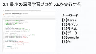
キーワード 【1】Keras 【2】モデル 【3】ラベル 【4】データ 【5】compile 【6】fit 2.1 最小の深層学習プログラムを実行する
14.
from keras.models import
Sequential from keras.layers import Dense, Activation from keras.utils import np_utils import numpy as np # ランダムデータの生成 data = np.random.random((1000, 784)) labels = np.random.randint(10, size=(1000, 1)) labels = np_utils.to_categorical(labels, 10) model = Sequential() model.add(Dense(64, activation='relu', input_dim=784)) model.add(Dense(64, activation='relu')) model.add(Dense(10, activation='softmax')) # モデルをコンパイルする model.compile(optimizer='rmsprop', loss='categorical_crossentropy', metrics=['accuracy']) # 学習を行う model.fit(data, labels) ニューラルネットワークの構成 データとラベルの設定 損失関数とオプティマイザーの設定 作成したラベルとデータを使って学習 2.1 最小の深層学習プログラム を実行する
15.
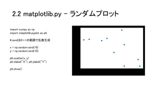
2.2 matplotlib.py –
ランダムプロット import numpy as np import matplotlib.pyplot as plt #.randは0~1の範囲で乱数生成 x = np.random.rand(10) y = np.random.rand(10) plt.scatter(x, y) plt.xlabel("X"), plt.ylabel("Y") plt.show()
16.
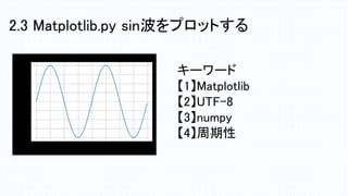
2.3 Matplotlib.py sin波をプロットする キーワード 【1】Matplotlib 【2】UTF-8 【3】numpy 【4】周期性
17.
# coding: utf-8 #
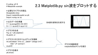
Matplotlib example # 必要なライブラリの読込 #matplotlib inline Import matplotlib.pyplot as plt Import numpy as np # 出力データの準備 T = np.arange(0.0, 2.0, 0.01) S = 1 + np.sin(2 * np.pi * t) # グラフの生成 Fig, ax = plt.subplots() Ax.plot(t, s) # グラフに付けるラベルとグリッドを描画 Ax.set(xlabel=‘time (s)’, ylabel=‘voltage (mV)’, title=‘JT seminar') ax.grid() # グラフの表示 plt.show() グラフの描画設定 matplotlibのpltメソッドを使う 2.3 Matplotlib.py sin波をプロットする SIN波の波形を生成する
18.
2.4 計算グラフの構築と実行 キーワード 【1】Tensorflow 【2】エポック 【3】セッション 【4】プレースホルダー 【5】アサイン
19.
#-*- coding:utf-8 -*- import
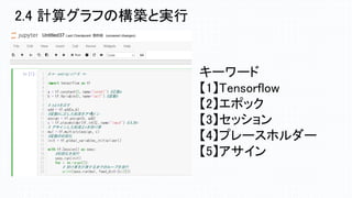
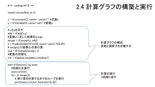
tensorflow as tf x = tf.constant(3, name=‘const1’) #定数x y = tf.Variable(0, name='val1') #変数y # xとyを足す add = tf.add(x,y) #変数yに足した結果をassign assign = tf.assign(y, add) z = tf.placeholder(tf.int32, name='input') #入力c # assignした結果とzを掛け算 mul = tf.multiply(assign, z) #変数の初期化 init = tf.global_variables_initializer() with tf.Session() as sess: #初期化を実行 sess.run(init) for i in range(3): # 掛け算を計算するまでのループを実行 print(sess.run(mul, feed_dict={c:3})) 計算グラフの構成 変数と演算子を定義する 計算の実行 3回繰り返す 2.4 計算グラフの構築と実行
20.
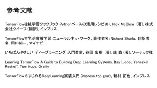
TensorFlow機械学習クックブック Pythonベースの活用レシピ60+, Nick
McClure (著), 株式 会社クイープ (翻訳), インプレス TensorFlowで学ぶ機械学習・ニューラルネットワーク、著作者名:Nishant Shukla、翻訳者 名:岡田佑一、マイナビ いちばんやさしい ディープラーニング 入門教室、谷岡 広樹 (著), 康 鑫 (著)、ソーテック社 Learning TensorFlow A Guide to Building Deep Learning Systems, Itay Lieder, Yehezkel Resheff, Tom Hope, Oreilly TensorFlowではじめるDeepLearning実装入門 (impress top gear)、新村 拓也、インプレス 参考文献
21.
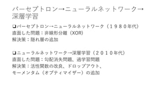
パーセプトロン→ニューラルネットワーク→ 深層学習 ❑パーセプトロン→ニューラルネットワーク(1980年代) 直面した問題:非線形分離(XOR) 解決策:隠れ層の追加 ❑ニューラルネットワーク→深層学習(2010年代) 直面した問題:勾配消失問題、過学習問題 解決策:活性関数の改良、ドロップアウト、 モーメンタム(オプティマイザー)の追加
22.
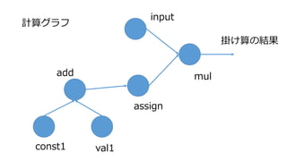
計算グラフ add val1const1 assign input mul 掛け算の結果
23.
③基本処理 3.1 線形回帰 3.2 非線形回帰 3.3
線形分離 3.4 非線形分離
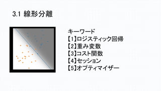
24.
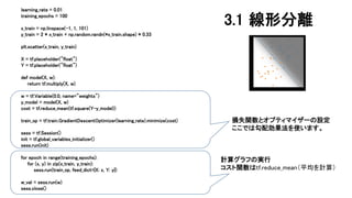
3.1 線形分離 キーワード 【1】ロジスティック回帰 【2】重み変数 【3】コスト関数 【4】セッション 【5】オプティマイザー
25.
learning_rate = 0.01 training_epochs
= 100 x_train = np.linspace(-1, 1, 101) y_train = 2 * x_train + np.random.randn(*x_train.shape) * 0.33 plt.scatter(x_train, y_train) X = tf.placeholder("float") Y = tf.placeholder("float") def model(X, w): return tf.multiply(X, w) w = tf.Variable(0.0, name="weights") y_model = model(X, w) cost = tf.reduce_mean(tf.square(Y-y_model)) train_op = tf.train.GradientDescentOptimizer(learning_rate).minimize(cost) sess = tf.Session() init = tf.global_variables_initializer() sess.run(init) for epoch in range(training_epochs): for (x, y) in zip(x_train, y_train): sess.run(train_op, feed_dict={X: x, Y: y}) w_val = sess.run(w) sess.close() 損失関数とオプティマイザーの設定 ここでは勾配効果法を使います。 計算グラフの実行 コスト関数はtf.reduce_mean(平均を計算) 3.1 線形分離
26.
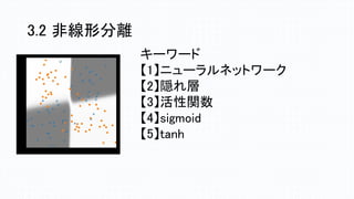
3.2 非線形分離 キーワード 【1】ニューラルネットワーク 【2】隠れ層 【3】活性関数 【4】sigmoid 【5】tanh
27.
num_units1 = 2 num_units2
= 2 x = tf.placeholder(tf.float32, [None, 2]) w1 = tf.Variable(tf.truncated_normal([2, num_units1])) b1 = tf.Variable(tf.zeros([num_units1])) hidden1 = tf.nn.tanh(tf.matmul(x, w1) + b1) w2 = tf.Variable(tf.truncated_normal([num_units1, num_units2])) b2 = tf.Variable(tf.zeros([num_units2])) hidden2 = tf.nn.tanh(tf.matmul(hidden1, w2) + b2) w0 = tf.Variable(tf.zeros([num_units2, 1])) b0 = tf.Variable(tf.zeros([1])) p = tf.nn.sigmoid(tf.matmul(hidden2, w0) + b0) t = tf.placeholder(tf.float32, [None, 1]) loss = -tf.reduce_sum(t*tf.log(p) + (1-t)*tf.log(1-p)) train_step = tf.train.GradientDescentOptimizer(0.001).minimize(loss) correct_prediction = tf.equal(tf.sign(p-0.5), tf.sign(t-0.5)) accuracy = tf.reduce_mean(tf.cast(correct_prediction, tf.float32)) sess = tf.Session() sess.run(tf.initialize_all_variables()) i = 0 for _ in range(2000): i += 1 sess.run(train_step, feed_dict={x:train_x, t:train_t}) if i % 100 == 0: loss_val, acc_val = sess.run( [loss, accuracy], feed_dict={x:train_x, t:train_t}) print ('Step: %d, Loss: %f, Accuracy: %f' % (i, loss_val, acc_val)) 三層モデルの設定 tanh関数とsigmoid関数を 使う 損失関数とオプティマイザー の設定 損失関数はreduce_sumを使う。 学習。誤差を正解率を ステップごとに表示。
28.
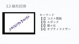
3.3 線形回帰 キーワード 【1】コスト関数 【2】エポック 【3】最小化 【4】オプティマイザー
29.
np.random.seed(20160512) n0, mu0, variance0
= 20, [10, 11], 20 data0 = multivariate_normal(mu0, np.eye(2)*variance0 ,n0) df0 = DataFrame(data0, columns=['x1','x2']) df0['t'] = 0 n1, mu1, variance1 = 15, [18, 20], 22 data1 = multivariate_normal(mu1, np.eye(2)*variance1 ,n1) df1 = DataFrame(data1, columns=['x1','x2']) df1['t'] = 1 df = pd.concat([df0, df1], ignore_index=True) train_set = df.reindex(permutation(df.index)).reset_index(drop=True) train_x = train_set[['x1','x2']].as_matrix() train_t = train_set['t'].as_matrix().reshape([len(train_set), 1]) x = tf.placeholder(tf.float32, [None, 2]) w = tf.Variable(tf.zeros([2, 1])) w0 = tf.Variable(tf.zeros([1])) f = tf.matmul(x, w) + w0 p = tf.sigmoid(f) t = tf.placeholder(tf.float32, [None, 1]) loss = -tf.reduce_sum(t*tf.log(p) + (1-t)*tf.log(1-p)) train_step = tf.train.AdamOptimizer().minimize(loss) correct_prediction = tf.equal(tf.sign(p-0.5), tf.sign(t-0.5)) accuracy = tf.reduce_mean(tf.cast(correct_prediction, tf.float32)) sess = tf.Session() sess.run(tf.initialize_all_variables()) i = 0 for _ in range(20000): i += 1 sess.run(train_step, feed_dict={x:train_x, t:train_t}) if i % 2000 == 0: loss_val, acc_val = sess.run( [loss, accuracy], feed_dict={x:train_x, t:train_t}) print ('Step: %d, Loss: %f, Accuracy: %f' % (i, loss_val, acc_val)) 学習 コスト関数と オプティマイザーの設定 AdamOptimizerを使う。
30.
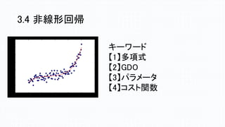
3.4 非線形回帰 キーワード 【1】多項式 【2】GDO 【3】パラメータ 【4】コスト関数
31.
learning_rate = 0.01 training_epochs
= 40 trX = np.linspace(-1, 1, 101) num_coeffs = 6 trY_coeffs = [1, 2, 3, 4, 5, 6] trY = 0 for i in range(num_coeffs): trY += trY_coeffs[i] * np.power(trX, i) trY += np.random.randn(*trX.shape) * 1.5 plt.scatter(trX, trY) plt.show() X = tf.placeholder("float") Y = tf.placeholder("float") def model(X, w): terms = [] for i in range(num_coeffs): term = tf.multiply(w[i], tf.pow(X, i)) terms.append(term) return tf.add_n(terms) w = tf.Variable([0.] * num_coeffs, name="parameters") y_model = model(X, w) cost = tf.reduce_sum(tf.square(Y-y_model)) train_op = tf.train.GradientDescentOptimizer(learning_rate).minimize(cost) sess = tf.Session() init = tf.global_variables_initializer() sess.run(init) for epoch in range(training_epochs): for (x, y) in zip(trX, trY): sess.run(train_op, feed_dict={X: x, Y: y}) w_val = sess.run(w) print(w_val) 学習 モデルの設定 多項式を決定する 6次の多項式 3.4 非線形回帰
32.
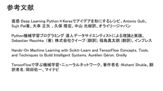
直感 Deep Learning
Python×Kerasでアイデアを形にするレシピ、Antonio Gulli、 Sujit Pal著、大串 正矢 、久保 隆宏、中山 光樹訳、オライリージャパン Python機械学習プログラミング 達人データサイエンティストによる理論と実践、 Sebastian Raschka (著), 株式会社クイープ (翻訳), 福島真太朗 (翻訳)、インプレス Hands-On Machine Learning with Scikit-Learn and TensorFlow Concepts, Tools, and Techniques to Build Intelligent Systems, Aurélien Géron, Oreilly TensorFlowで学ぶ機械学習・ニューラルネットワーク、著作者名:Nishant Shukla、翻 訳者名:岡田佑一、マイナビ 参考文献
33.
④sin波とRNN 4.1 リカレントニューラルネットワークの解説 4.2 Tensorflowで実装する 4.3
Kerasで実装する
34.
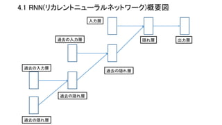
4.1 RNN(リカレントニューラルネットワーク)概要図 過去の隠れ層 過去の入力層 過去の入力層 過去の隠れ層 出力層 過去の隠れ層 隠れ層 入力層
35.
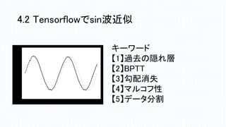
4.2 Tensorflowでsin波近似 キーワード 【1】過去の隠れ層 【2】BPTT 【3】勾配消失 【4】マルコフ性 【5】データ分割
36.
def inference(x, n_batch,
maxlen=None, n_hidden=None, n_out=None): def weight_variable(shape): initial = tf.truncated_normal(shape, stddev=0.01) return tf.Variable(initial) def bias_variable(shape): initial = tf.zeros(shape, dtype=tf.float32) return tf.Variable(initial) cell = tf.nn.rnn_cell.BasicRNNCell(n_hidden) initial_state = cell.zero_state(n_batch, tf.float32) state = initial_state outputs = [] # 過去の隠れ層の出力を保存 with tf.variable_scope('RNN'): for t in range(maxlen): if t > 0: tf.get_variable_scope().reuse_variables() (cell_output, state) = cell(x[:, t, :], state) outputs.append(cell_output) output = outputs[-1] V = weight_variable([n_hidden, n_out]) c = bias_variable([n_out]) y = tf.matmul(output, V) + c # 線形活性 return y リカレントニューラルネットワーク層を構成 時系列に沿った状態を保持しておくための実装 活性関数の設定 内部で state( 隠れ層の状態)を保持し、 時間軸に沿った順伝播を計算する
37.
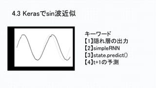
4.3 Kerasでsin波近似 キーワード 【1】隠れ層の出力 【2】simpleRNN 【3】state.predict() 【4】t+1の予測
38.
model = Sequential() model.add(SimpleRNN(n_hidden, kernel_initializer=weight_variable, input_shape=(maxlen,
n_in))) model.add(Dense(n_out, kernel_initializer=weight_variable)) model.add(Activation('linear')) optimizer = Adam(lr=0.001, beta_1=0.9, beta_2=0.999) model.compile(loss='mean_squared_error', optimizer=optimizer) '''s モデル学習 ''' epochs = 500 batch_size = 10 model.fit(X_train, Y_train, batch_size=batch_size, epochs=epochs, validation_data=(X_validation, Y_validation), callbacks=[early_stopping]) モデルとオプティマイザーの設定 隠れ層をsimpleRNNに設定 学習 Early stopping:学習が進んで精度の 向上がこれ以上見込めないとなったら、 そこで学習を止める」
39.
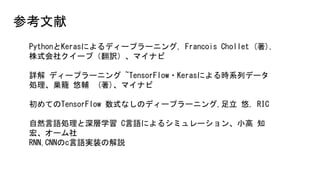
PythonとKerasによるディープラーニング, Francois Chollet
(著), 株式会社クイープ(翻訳)、マイナビ 詳解 ディープラーニング ~TensorFlow・Kerasによる時系列データ 処理、巣籠 悠輔 (著)、マイナビ 初めてのTensorFlow 数式なしのディープラーニング,足立 悠, RIC 自然言語処理と深層学習 C言語によるシミュレーション、小高 知 宏、オーム社 RNN,CNNのc言語実装の解説 参考文献
40.
⑤NMISTとCNN 5.1 畳み込みニューラルネットワークの説明 5.2 Tensorflowで実装 5.3
Kerasで実装
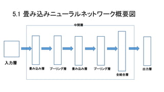
41.
5.1 畳み込みニューラルネットワーク概要図 入力層 畳み込み層プーリング層畳み込み層 プーリング層 全結合層 出力層 中間層
42.
# Initialize Model
Operations def my_conv_net(conv_input_data): # 第1層 conv1 = tf.nn.conv2d(conv_input_data, conv1_weight, strides=[1, 1, 1, 1], padding='SAME') relu1 = tf.nn.relu(tf.nn.bias_add(conv1, conv1_bias)) max_pool1 = tf.nn.max_pool(relu1, ksize=[1, max_pool_size1, max_pool_size1, 1], strides=[1, max_pool_size1, max_pool_size1, 1], padding='SAME') # 第2層 conv2 = tf.nn.conv2d(max_pool1, conv2_weight, strides=[1, 1, 1, 1], padding='SAME') relu2 = tf.nn.relu(tf.nn.bias_add(conv2, conv2_bias)) max_pool2 = tf.nn.max_pool(relu2, ksize=[1, max_pool_size2, max_pool_size2, 1], strides=[1, max_pool_size2, max_pool_size2, 1], padding='SAME') final_conv_shape = max_pool2.get_shape().as_list() final_shape = final_conv_shape[1] * final_conv_shape[2] * final_conv_shape[3] flat_output = tf.reshape(max_pool2, [final_conv_shape[0], final_shape]) fully_connected1 = tf.nn.relu(tf.add(tf.matmul(flat_output, full1_weight), full1_bias)) final_model_output = tf.add(tf.matmul(fully_connected1, full2_weight), full2_bias) return final_model_output 畳み込み第1層と第2層の設定 活性関数にreluを使う プーリング層と全結合層の設定 結合層の第1層はrelu, 第2層は乗算を用いる
43.
# モデルを作成 model =
Sequential() model.add(Dense(512, input_shape=(784, ))) model.add(Activation('relu')) model.add(Dropout(0.2)) model.add(Dense(512)) model.add(Activation('relu')) model.add(Dropout(0.2)) model.add(Dense(10)) model.add(Activation('softmax')) # サマリーを出力 model.summary() # モデルのコンパイル model.compile(loss='categorical_crossentropy', optimizer=RMSprop(), metrics=['accuracy']) es = EarlyStopping(monitor='val_loss', patience=2) csv_logger = CSVLogger('training.log') hist = model.fit(x_train, y_train, batch_size=batch_size, epochs=epochs, verbose=1, validation_split=0.1, callbacks=[es, csv_logger]) モデルの設定 第1層、第2層にrelu、第3層にsoftmaxを 用いる 学習
44.
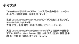
TensorFlowで学ぶディープラーニング入門~畳み込みニューラル ネットワーク徹底解説、中井悦司、マイナビ 直感 Deep Learning
Python×Kerasでアイデアを形にするレシピ、 Antonio Gulli、Sujit Pal著、 大串 正矢 、久保 隆宏、中山 光樹訳、オライリージャパン 実践 Deep Learning PythonとTensorFlowで学ぶ次世代の機械学 習アルゴリズム、Nikhil Buduma (著), 太田 満久 (監修), 藤原 秀平 (監修), 牧野 聡 (翻訳)、オライリージャパン 参考文献
Download


![from keras.models import Sequential
from keras.layers import Dense, Activation
from keras.utils import np_utils
import numpy as np
# ランダムデータの生成
data = np.random.random((1000, 784))
labels = np.random.randint(10, size=(1000, 1))
labels = np_utils.to_categorical(labels, 10)
model = Sequential()
model.add(Dense(64, activation='relu', input_dim=784))
model.add(Dense(64, activation='relu'))
model.add(Dense(10, activation='softmax'))
# モデルをコンパイルする
model.compile(optimizer='rmsprop',
loss='categorical_crossentropy',
metrics=['accuracy'])
# 学習を行う
model.fit(data, labels)
ニューラルネットワークの構成
データとラベルの設定
損失関数とオプティマイザーの設定
作成したラベルとデータを使って学習
2.1 最小の深層学習プログラム
を実行する](https://image.slidesharecdn.com/tensorflow-keras-handson-tutorial-2018-11-200729102550/85/Tensorflow-Keras-14-320.jpg)

![num_units1 = 2
num_units2 = 2
x = tf.placeholder(tf.float32, [None, 2])
w1 = tf.Variable(tf.truncated_normal([2, num_units1]))
b1 = tf.Variable(tf.zeros([num_units1]))
hidden1 = tf.nn.tanh(tf.matmul(x, w1) + b1)
w2 = tf.Variable(tf.truncated_normal([num_units1, num_units2]))
b2 = tf.Variable(tf.zeros([num_units2]))
hidden2 = tf.nn.tanh(tf.matmul(hidden1, w2) + b2)
w0 = tf.Variable(tf.zeros([num_units2, 1]))
b0 = tf.Variable(tf.zeros([1]))
p = tf.nn.sigmoid(tf.matmul(hidden2, w0) + b0)
t = tf.placeholder(tf.float32, [None, 1])
loss = -tf.reduce_sum(t*tf.log(p) + (1-t)*tf.log(1-p))
train_step = tf.train.GradientDescentOptimizer(0.001).minimize(loss)
correct_prediction = tf.equal(tf.sign(p-0.5), tf.sign(t-0.5))
accuracy = tf.reduce_mean(tf.cast(correct_prediction, tf.float32))
sess = tf.Session()
sess.run(tf.initialize_all_variables())
i = 0
for _ in range(2000):
i += 1
sess.run(train_step, feed_dict={x:train_x, t:train_t})
if i % 100 == 0:
loss_val, acc_val = sess.run(
[loss, accuracy], feed_dict={x:train_x, t:train_t})
print ('Step: %d, Loss: %f, Accuracy: %f'
% (i, loss_val, acc_val))
三層モデルの設定
tanh関数とsigmoid関数を
使う
損失関数とオプティマイザー
の設定
損失関数はreduce_sumを使う。
学習。誤差を正解率を
ステップごとに表示。](https://image.slidesharecdn.com/tensorflow-keras-handson-tutorial-2018-11-200729102550/85/Tensorflow-Keras-27-320.jpg)
![np.random.seed(20160512)
n0, mu0, variance0 = 20, [10, 11], 20
data0 = multivariate_normal(mu0, np.eye(2)*variance0 ,n0)
df0 = DataFrame(data0, columns=['x1','x2'])
df0['t'] = 0
n1, mu1, variance1 = 15, [18, 20], 22
data1 = multivariate_normal(mu1, np.eye(2)*variance1 ,n1)
df1 = DataFrame(data1, columns=['x1','x2'])
df1['t'] = 1
df = pd.concat([df0, df1], ignore_index=True)
train_set = df.reindex(permutation(df.index)).reset_index(drop=True)
train_x = train_set[['x1','x2']].as_matrix()
train_t = train_set['t'].as_matrix().reshape([len(train_set), 1])
x = tf.placeholder(tf.float32, [None, 2])
w = tf.Variable(tf.zeros([2, 1]))
w0 = tf.Variable(tf.zeros([1]))
f = tf.matmul(x, w) + w0
p = tf.sigmoid(f)
t = tf.placeholder(tf.float32, [None, 1])
loss = -tf.reduce_sum(t*tf.log(p) + (1-t)*tf.log(1-p))
train_step = tf.train.AdamOptimizer().minimize(loss)
correct_prediction = tf.equal(tf.sign(p-0.5), tf.sign(t-0.5))
accuracy = tf.reduce_mean(tf.cast(correct_prediction, tf.float32))
sess = tf.Session()
sess.run(tf.initialize_all_variables())
i = 0
for _ in range(20000):
i += 1
sess.run(train_step, feed_dict={x:train_x, t:train_t})
if i % 2000 == 0:
loss_val, acc_val = sess.run(
[loss, accuracy], feed_dict={x:train_x, t:train_t})
print ('Step: %d, Loss: %f, Accuracy: %f'
% (i, loss_val, acc_val))
学習
コスト関数と
オプティマイザーの設定
AdamOptimizerを使う。](https://image.slidesharecdn.com/tensorflow-keras-handson-tutorial-2018-11-200729102550/85/Tensorflow-Keras-29-320.jpg)
![learning_rate = 0.01
training_epochs = 40
trX = np.linspace(-1, 1, 101)
num_coeffs = 6
trY_coeffs = [1, 2, 3, 4, 5, 6]
trY = 0
for i in range(num_coeffs):
trY += trY_coeffs[i] * np.power(trX, i)
trY += np.random.randn(*trX.shape) * 1.5
plt.scatter(trX, trY)
plt.show()
X = tf.placeholder("float")
Y = tf.placeholder("float")
def model(X, w):
terms = []
for i in range(num_coeffs):
term = tf.multiply(w[i], tf.pow(X, i))
terms.append(term)
return tf.add_n(terms)
w = tf.Variable([0.] * num_coeffs, name="parameters")
y_model = model(X, w)
cost = tf.reduce_sum(tf.square(Y-y_model))
train_op = tf.train.GradientDescentOptimizer(learning_rate).minimize(cost)
sess = tf.Session()
init = tf.global_variables_initializer()
sess.run(init)
for epoch in range(training_epochs):
for (x, y) in zip(trX, trY):
sess.run(train_op, feed_dict={X: x, Y: y})
w_val = sess.run(w)
print(w_val)
学習
モデルの設定
多項式を決定する
6次の多項式
3.4 非線形回帰](https://image.slidesharecdn.com/tensorflow-keras-handson-tutorial-2018-11-200729102550/85/Tensorflow-Keras-31-320.jpg)

![def inference(x, n_batch, maxlen=None, n_hidden=None, n_out=None):
def weight_variable(shape):
initial = tf.truncated_normal(shape, stddev=0.01)
return tf.Variable(initial)
def bias_variable(shape):
initial = tf.zeros(shape, dtype=tf.float32)
return tf.Variable(initial)
cell = tf.nn.rnn_cell.BasicRNNCell(n_hidden)
initial_state = cell.zero_state(n_batch, tf.float32)
state = initial_state
outputs = [] # 過去の隠れ層の出力を保存
with tf.variable_scope('RNN'):
for t in range(maxlen):
if t > 0:
tf.get_variable_scope().reuse_variables()
(cell_output, state) = cell(x[:, t, :], state)
outputs.append(cell_output)
output = outputs[-1]
V = weight_variable([n_hidden, n_out])
c = bias_variable([n_out])
y = tf.matmul(output, V) + c # 線形活性
return y
リカレントニューラルネットワーク層を構成
時系列に沿った状態を保持しておくための実装
活性関数の設定
内部で state( 隠れ層の状態)を保持し、
時間軸に沿った順伝播を計算する](https://image.slidesharecdn.com/tensorflow-keras-handson-tutorial-2018-11-200729102550/85/Tensorflow-Keras-36-320.jpg)
![model = Sequential()
model.add(SimpleRNN(n_hidden,
kernel_initializer=weight_variable,
input_shape=(maxlen, n_in)))
model.add(Dense(n_out, kernel_initializer=weight_variable))
model.add(Activation('linear'))
optimizer = Adam(lr=0.001, beta_1=0.9, beta_2=0.999)
model.compile(loss='mean_squared_error',
optimizer=optimizer)
'''s
モデル学習
'''
epochs = 500
batch_size = 10
model.fit(X_train, Y_train,
batch_size=batch_size,
epochs=epochs,
validation_data=(X_validation, Y_validation),
callbacks=[early_stopping])
モデルとオプティマイザーの設定
隠れ層をsimpleRNNに設定
学習
Early stopping:学習が進んで精度の
向上がこれ以上見込めないとなったら、
そこで学習を止める」](https://image.slidesharecdn.com/tensorflow-keras-handson-tutorial-2018-11-200729102550/85/Tensorflow-Keras-38-320.jpg)

![# Initialize Model Operations
def my_conv_net(conv_input_data):
# 第1層
conv1 = tf.nn.conv2d(conv_input_data, conv1_weight, strides=[1, 1, 1, 1], padding='SAME')
relu1 = tf.nn.relu(tf.nn.bias_add(conv1, conv1_bias))
max_pool1 = tf.nn.max_pool(relu1, ksize=[1, max_pool_size1, max_pool_size1, 1],
strides=[1, max_pool_size1, max_pool_size1, 1], padding='SAME')
# 第2層
conv2 = tf.nn.conv2d(max_pool1, conv2_weight, strides=[1, 1, 1, 1], padding='SAME')
relu2 = tf.nn.relu(tf.nn.bias_add(conv2, conv2_bias))
max_pool2 = tf.nn.max_pool(relu2, ksize=[1, max_pool_size2, max_pool_size2, 1],
strides=[1, max_pool_size2, max_pool_size2, 1], padding='SAME')
final_conv_shape = max_pool2.get_shape().as_list()
final_shape = final_conv_shape[1] * final_conv_shape[2] * final_conv_shape[3]
flat_output = tf.reshape(max_pool2, [final_conv_shape[0], final_shape])
fully_connected1 = tf.nn.relu(tf.add(tf.matmul(flat_output, full1_weight), full1_bias))
final_model_output = tf.add(tf.matmul(fully_connected1, full2_weight), full2_bias)
return final_model_output
畳み込み第1層と第2層の設定
活性関数にreluを使う
プーリング層と全結合層の設定
結合層の第1層はrelu,
第2層は乗算を用いる](https://image.slidesharecdn.com/tensorflow-keras-handson-tutorial-2018-11-200729102550/85/Tensorflow-Keras-42-320.jpg)
![# モデルを作成
model = Sequential()
model.add(Dense(512, input_shape=(784, )))
model.add(Activation('relu'))
model.add(Dropout(0.2))
model.add(Dense(512))
model.add(Activation('relu'))
model.add(Dropout(0.2))
model.add(Dense(10))
model.add(Activation('softmax'))
# サマリーを出力
model.summary()
# モデルのコンパイル
model.compile(loss='categorical_crossentropy',
optimizer=RMSprop(),
metrics=['accuracy'])
es = EarlyStopping(monitor='val_loss', patience=2)
csv_logger = CSVLogger('training.log')
hist = model.fit(x_train, y_train,
batch_size=batch_size,
epochs=epochs,
verbose=1,
validation_split=0.1,
callbacks=[es, csv_logger])
モデルの設定
第1層、第2層にrelu、第3層にsoftmaxを
用いる
学習](https://image.slidesharecdn.com/tensorflow-keras-handson-tutorial-2018-11-200729102550/85/Tensorflow-Keras-43-320.jpg)


![[第2版]Python機械学習プログラミング 第16章](https://cdn.slidesharecdn.com/ss_thumbnails/16-190318023255-thumbnail.jpg?width=640&height=640&fit=bounds)


![[第2版]Python機械学習プログラミング 第13章](https://cdn.slidesharecdn.com/ss_thumbnails/13-190318023252-thumbnail.jpg?width=640&height=640&fit=bounds)
![[第2版]Python機械学習プログラミング 第14章](https://cdn.slidesharecdn.com/ss_thumbnails/14-190318023253-thumbnail.jpg?width=640&height=640&fit=bounds)


![[DL Hacks] Deterministic Variational Inference for RobustBayesian Neural Netw...](https://cdn.slidesharecdn.com/ss_thumbnails/adobepdffile2-190628001736-thumbnail.jpg?width=640&height=640&fit=bounds)


