The document explores the impact of temperature on a new type of ferroelectric interfaced negative capacitance double gate junctionless accumulation mode field effect transistor (nc-dg-jam-fet). It presents a compact model that analyzes various performance parameters, including surface potential and gain, as temperature varies between 200 to 500 K, revealing significant effects such as increased sub-threshold swing and loss of gain at high temperatures. The findings suggest that while nc-dg-jam-fets are promising for low power applications, temperature management is crucial for optimizing their performance.

1. royalsocietypublishing.org/journal/rspa
Research
Cite this article: Yadav S, Rewari S, Pandey R.
2023 Impact of temperature on a ferroelectric
interfaced negative capacitance double gate
junctionless accumulation mode field effect
transistor-compact model. Proc.R.Soc.A 479:
20220528.
https://doi.org/10.1098/rspa.2022.0528
Received: 1 August 2022
Accepted: 3 February 2023
Subject Areas:
nanotechnology, solid-state physics,
mathematical modelling
Keywords:
ferroelectric material, junctionless
accumulation mode, negative capacitance,
temperature
Author for correspondence:
Snehlata Yadav
e-mail: snehlata_2k19phdec03@dtu.ac.in
Impact of temperature on a
ferroelectric interfaced
negative capacitance double
gatejunctionlessaccumulation
mode field effect
transistor-compact model
Snehlata Yadav, Sonam Rewari and
Rajeshwari Pandey
Department of Electronics and Communication Engineering, Delhi
Technological University, Delhi, Delhi 110042, India
SY, 0000-0003-3929-2306
Ferroelectric interfaced negative capacitance field
effect transistors are gaining popularity for low
power applications; however, as temperature is
a constant influencing factor, further study is
required to comprehend how these devices are
influenced. Through a proposed compact model,
this paper analytically investigates the influence of
temperature on a ferroelectric interfaced negative
capacitance double gate junctionless accumulation
mode field effect transistor. This device integrates
the benefits of negative capacitance with the
junctionless accumulation mode structure. An
extensive comparison of the proposed device is
made with the existing structure to evaluate the
benefits offered by the ferroelectric layer at different
temperatures. The Landau–Khalatnikov equation and
Pao–Sah integral are employed to obtain the surface
potential and drain current model with temperature
variation. Various key parameters of the device have
been analysed extensively by varying the temperature
from 200 to 500 K. It has been found that internal
voltage amplification declines as temperature rises,
but the sub-threshold swing increases from 46 to
72 mV decade−1 with an increase in temperature.
Additionally, with a progressive rise in temperature,
the loss of gain and degradation of gate capacitance
are observed.
2023 The Author(s) Published by the Royal Society. All rights reserved.
Downloaded
from
https://royalsocietypublishing.org/
on
01
March
2023

2. 2
royalsocietypublishing.org/journal/rspa
Proc.
R.
Soc.
A
479:
20220528
.
.
.
.
.
.
.
.
.
.
.
.
.
.
.
.
.
.
.
.
.
.
.
.
.
.
.
.
.
.
.
.
.
.
.
.
.
.
.
.
.
.
.
.
.
.
.
.
.
.
.
.
.
.
.
.
.
.
1. Introduction
There has been an intensive study on ferroelectric devices with negative capacitance, especially
in the last decade. This is attributed to the fact that these devices drop the sub-threshold
swing (SS) below the Boltzmann tyranny, hence reducing off-state leakage current [1]. To further
comprehend the theories and modelling approach, simulations of the negative capacitance field
effect transistor (NC-FET) have been used effectively in addition to practical demonstrations [2].
Analytical methods have been used to solve the Landau–Khalatnikov (L-K) equation [3,4] to
illustrate the NC effect, temperature influence on NC-FET, the design process of NC-FET and the
design of ferroelectric capacitance. However, these analyses were limited to negative capacitance-
based junctionless transistors (JLTs). Although JLTs ease the fabrication complexity, these have
some major limitations, such as higher gate work function in order to turn off the device, lower
drain current and transconductance. Therefore, a newly modified structure called JAM-MOSFET
was introduced to eliminate these drawbacks. In JAM-MOSFET, JAM stands for junctionless
accumulation mode and MOSFET is an acronym for metal oxide semiconductor field effect
transistor. JAM-MOSFET has an n +-n-n + homojunction and is a single-doping-type structure.
The doping concentration of the channel region is lower than that of the source/drain region.
Higher doping is used in the source/drain areas of the JAM-MOSFET to boost conductivity
and prevent high parasitic access resistance. The lower doping in the channel region fixes the
issue of carrier mobility degradation and offers better transconductance and On-state current.
The carriers in a JAM-MOSFET accumulate at the source–channel–drain junctions in a manner
akin to an ohmic contact [5,6]. Owing to the merits of both NC and JAM structures, the negative
capacitance double gate junctionless accumulation mode field effect transistor (NC-DG-JAM-FET)
is proposed.
For any device, temperature plays a crucial role in diverse applications like memories,
microcontrollers, sensors, converters and so on [7]. In addition to this, ferroelectric materials are
susceptible to changes in temperature because ferroelectric material properties are based on Gibbs
free energy, and it captures the NC fundamental property up to Curie temperature. Increasing
the temperature above the Curie point causes the ferroelectric material to transition into a non-
ferroelectric or paraelectric phase [8]. The L-K explanation of phase transition can be theoretically
understood in terms of Gibbs Free Energy: U = αP2 + βP4 + γ P6, where α = α0 (T − Tc), P
denotes the polarization and Tc is the Curie temperature. Here, α0, β and γ are constants for
the given ferroelectric material, hafnium zirconium oxide (HZO) (i.e. α0 = −2.5 × 109 Vm C−1,
β = 6.0 × 1010 Vm5 C−3 and γ = 1.5 × 1011 Vm9 C−5 [9]). Since α < 0 which implies T < Tc, the
phase transition for ferroelectric material does not occur. From the previous report, Mueller et al.
demonstrated that HZO thin films have a stable ferroelectric phase in a temperature range from
100 to 400 K. The phase transition takes place above 450 K. Therefore, the Curie temperature of
HZO material is above 450 K [10]. Hence, a temperature-dependent compact model of the NC-
DG-JAM-FET is developed in this work, and a thorough investigation is done on its various
performance parameters for temperatures ranging from 200 to 500 K. These parameters include
surface potential, gain, capacitance, drain current, threshold voltage and SS.
Section 2 describes the device structure and characteristic parameters to obtain its key traits
at different temperatures. The proposed compact model in §3 integrates the benefits of both
negative capacitance and JAM-FET for improved device performance. The results and discussion
are covered in §4. Section 5 concludes the work.
2. Proposed device
(a) Device structure and simulation
The proposed device (NC-DG-JAM-FET) uses an n-type doped, symmetric double gate
junctionless accumulation mode transistor with HZO as the ferroelectric layer and an insulator
Downloaded
from
https://royalsocietypublishing.org/
on
01
March
2023

3. 3
royalsocietypublishing.org/journal/rspa
Proc.
R.
Soc.
A
479:
20220528
.
.
.
.
.
.
.
.
.
.
.
.
.
.
.
.
.
.
.
.
.
.
.
.
.
.
.
.
.
.
.
.
.
.
.
.
.
.
.
.
.
.
.
.
.
.
.
.
.
.
.
.
.
.
.
.
.
.
gate metal
gate metal
gate
gate
ferroelectric layer
ferroelectric layer
ferroelectric
energy
(U)
insulator layer
insulator layer
L
channel
N
source
tIL
tFE
tFE
tCH
VG
CFE
CIL
CSC
tIL
y
x N+
drain
N+
SC
IL
FE
M
(a) (b) (c)
(e)
(d)
0
10
–10
–20
20
0.5 1.0 1.5
0
electric field (MV cm–1)
–1.5 –1.0 –0.5
0
0.8
C < 0
NC region
(C < 0)
–1.6
–0.8
–2.4
–20 –10
FE FE
IL IL
EV
–TCH/2 TCH/2
0
Ei
EC
N doped Si
Ei
EF
φSP
φCP
0
polarization (P)
polarization
(C
cm
–2
)
10 20
Figure 1. (a) Schematic diagram of the NC-DG-JAM-FET. (b) MFIS structure and its equivalent capacitance model. (c) The
double-wellferroelectricenergyversuspolarizationusingLKtheory.(d)Ferroelectricpolarizationasafunctionofelectricfield.
(e) Energy bands that are normal to the channel are obtained when the device is operated in the NC region.
layer between the silicon channel and the ferroelectric layer, as shown in figure 1a. The thicknesses
of the ferroelectric (tFE), insulator (tIL) and channel layers (tCH) are taken as 5, 1 and 10 nm,
respectively. In ferroelectric FETs, it is crucial to properly tune the thickness of the ferroelectric
layer to obtain high gain and minimum hysteresis. Here, 5 nm HZO is taken as the critical
thickness for hysteresis-free operation and guarantees SS < 60 mV decade−1 [11]. The thickness
of the insulator layer is usually considered in nanometres. Here, it is taken as 1 nm to achieve
a small area and low power consumption and also allows a smaller voltage to induce the same
channel charge and drive current [12]. The quantum mechanical effects have been neglected in
the TCAD simulations since the channel thickness is 10 nm [13]. Since the device configuration is
of metal-ferroelectric-insulator-semiconductor type, its equivalent capacitive model is shown in
figure 1b. To realize the JAM structure, doping concentration at the source–drain and the channel
region are taken as 1 × 1019 cm−3 and 1 × 1017 cm−3, respectively.
Since the JAM structure requires a low work function, therefore, titanium nitride (TiN) is taken
as gate metal whose work function is 4.65 eV. The simulations are performed using the Silvaco
ATLAS TCAD simulator, with the Lombardi CVT model, Shockley–Read–Hall recombination,
Fermi, Ferro and L-K models [14].
The concept of NC can be understood by considering the ferroelectric’s free energy density.
A ferroelectric material is traditionally modelled based on Landau–Ginzburg–Devonshire theory
[15]. In this theory, a ferroelectric is explained by a double-well energy density (U) as a function
of polarization (P) [16] depicted in figure 1c and expressed as
U = αP2
+ βP4
+ γ P6
− E.P, (2.1)
where E is the external applied electric field, and α, β and γ are ferroelectric material parameters
typical of HZO. By differentiating U with respect to P and setting dU/dP = 0, the following L-K
Downloaded
from
https://royalsocietypublishing.org/
on
01
March
2023

4. 4
royalsocietypublishing.org/journal/rspa
Proc.
R.
Soc.
A
479:
20220528
.
.
.
.
.
.
.
.
.
.
.
.
.
.
.
.
.
.
.
.
.
.
.
.
.
.
.
.
.
.
.
.
.
.
.
.
.
.
.
.
.
.
.
.
.
.
.
.
.
.
.
.
.
.
.
.
.
.
equation [17] is obtained:
E = 2αP + 4βP3
+ 6γ P5
. (2.2)
The S-shaped P-E characteristic curve is obtained from the above equation, as depicted in
figure 1d. This S-shaped curve displays an unstable negative slope (dP/dE) area from which the
negative capacitance (C < 0) arises because capacitance (C) is proportional to the slope, dP/dE.
When the device is used in the NC region, the relevant energy bands are shown in figure 1e
in the direction normal to the channel. N-doped and curved upward in the accumulation mode
is the channel area. The analytically derived surface and centre potentials are denoted by the
symbols φSP and φCP. Ei is referred to as the intrinsic Fermi level, EC and EV are the conduction
band and valence band, respectively, and the energy band gap is determined by the difference
between them. This energy gap is also used to calculate silicon’s work function.
(b) Device fabrication and calibration
The proposed device (NC-DG-JAM-FET), based on ferroelectric insulators, is easier to fabricate,
with important fabrication processes being phosphorous implantation to generate the channel
and source/drain areas, accompanied by rapid thermal annealing that enables dopant activation.
Using atomic layer deposition, a doped ferroelectric layer is formed on a SiO2 interface
layer, followed by the deposition of a metal gate using physical vapour deposition, and then
ferroelectric films can be crystallized after metal annealing. These fabrication techniques for
ferroelectric-based devices have been experimentally proven [18]. The fabrication steps are shown
in figure 2a. The experimental research work under identical device dimensions is used to
calibrate this research work properly. To date, there are no experimental data in the literature for
the ferroelectric JAM-FET and that makes our proposed work more novel. However, to validate
and make our model more reliable, we have compared the simulation (realized using a Silvaco
ATLAS device simulator) with experimental data of the JAM-FET [19] and ferroelectric FET [20],
respectively. It is so found from figure 2b–d that the experimental results are near to our simulated
results.
3. Temperature-dependent compact modelling
The channel has a number of electrostatic properties whose fluctuation along the channel is quite
interesting. The gradual-channel approximation is found in terms of the width of the conductive
channel [21]. It provides the results for the potential inside the conductive channel and the drain
current of an n-channel device. Therefore, by employing Pao–Sah gradual-channel approximation
[22] and considering only mobile charges, the Poisson equation in the channel region is expressed
as
∂2φ(x, T)
∂x2
=
−qND
εsi
(1 − e(φ−V/(kT/q))
), (3.1)
where φ represents the channel potential and is a function of temperature, x represents the
distance along the vertical direction, k is the Boltzmann constant, T is the temperature in Kelvin
(K) and ND is the channel doping concentration. εsi, q and V represent the silicon permittivity,
electronic charge and electron quasi-Fermi potential, respectively. To obtain an expression for the
channel potential, the parabolic potential approximation as in [23,24] is applied in equation (3.1)
and represented by the following expression:
φ(x, T) = (φSP(x, T) − φCP(x, T))
4x2
t2
CH
+ φCP(x, T), (3.2)
where φSP and φCP are the surface potential and centre potential, respectively. The solutions
to these temperature-dependent parameters may be attained by administering these boundary
conditions:
Downloaded
from
https://royalsocietypublishing.org/
on
01
March
2023

5. 5
royalsocietypublishing.org/journal/rspa
Proc.
R.
Soc.
A
479:
20220528
.
.
.
.
.
.
.
.
.
.
.
.
.
.
.
.
.
.
.
.
.
.
.
.
.
.
.
.
.
.
.
.
.
.
.
.
.
.
.
.
.
.
.
.
.
.
.
.
.
.
.
.
.
.
.
.
.
.
(b)
(a)
(d)
(c)
0.5 1.0 1.5 2.0
0
VGS (V)
0.5 1.0 1.5 2.0
0
VD (V)
I
D
(A)
I
D
(A)
VDS = 1.0 V
VDS = 0.5 V
tFE = 1.8 nm
tIL = 2 nm
VDS = 0.1 V
VGS = 1.5 V
VGS = 1.0 V
–1.0
10–12
10–11
10–10
10–9
10–8
10–7
10–6
10–5
drain
current
I
D
(A)
10–12
10–11
10–10
10–9
10–8
10–7
10–6
10–5
line: experimental
symbol: simulation
line: experimental
simulation
experimental
symbol: simulation
–0.5
0
0.5
1.0
1.5
2.0
1.0
0.8
0.6
0.4
–0.4 0.2
–0.2
gate voltage VGS (V)
0
bulk silicon wafer
phosphorous implantation for
source/drain and channel
regions formation
rapid thermal annealing to
activate the dopant
the doped ferroelectric layer
deposition by atomic layer
deposition (ALD)
metal gate formation by
physical vapour deposition
(PVD)
post annealing to crystallize
ferroelectric films
Figure 2. (a) Fabrication steps of the proposed device. Calibration of simulated data with experimental data of (b) transfer
function of the ferroelectric FET, (c) transfer function of the JAM-FET and (d) output characteristics of the JAM-FET.
φ(x = 0, T) = φCP, (3.3)
dφ(x, T)
dx
x=0
= 0, (3.4)
φ
x =
tCH
2
, T
= φSP
tCH
2
, T
(3.5)
and
dφ(x, T)
dx
x=
tCH
2
=
4(φSP((tCH/2), T) − φCP)
tCH
. (3.6)
The relationships among φSP, φCP and the gate voltage (VGS) can be achieved by employing a
boundary condition and Gauss’s law at the interface as follows:
CTOT(VGS − VFB − φSP(x, T) =
4εsi
tCH
(φSP(x, T) − φCP), (3.7)
where
CTOT =
εFEεsi
(tFEεIL + εFEtIL)
. (3.8)
The total gate capacitance (CTOT) is expressed in terms of ferroelectric permittivity (εFE),
insulator permittivity (εIL), silicon permittivity (εsi), thicknesses of ferroelectric (tFE) and insulator
(tIL) layers. Since the source/drain portions of JAM-FETs have higher doping concentrations
than the channel region, a built-in potential (Vbi), exists at the source–channel and channel–drain
interfaces [25]:
Vbi =
kT
q
ln
N+
D
ND
, (3.9)
where N+
D is the doping concentration in source–drain regions. Hence, its effect on the
temperature-dependent parameters such as silicon’s work function (φsi) and flat-band voltage
Downloaded
from
https://royalsocietypublishing.org/
on
01
March
2023

6. 6
royalsocietypublishing.org/journal/rspa
Proc.
R.
Soc.
A
479:
20220528
.
.
.
.
.
.
.
.
.
.
.
.
.
.
.
.
.
.
.
.
.
.
.
.
.
.
.
.
.
.
.
.
.
.
.
.
.
.
.
.
.
.
.
.
.
.
.
.
.
.
.
.
.
.
.
.
.
.
(VFB) is given below:
φsi(T) = χ +
Eg
2
− Vbi (3.10)
and
VFB(T) = φM − φsi(T), (3.11)
where φM depicts the gate metal work function, χ depicts the electron affinity, Eg depicts the
energy band gap and ND is the doping concentration in the channel region. There are two
unknowns φSP and φCP in (3.7), so another expression relating φSP and φCP is needed to obtain a
solution. Therefore, by integrating (3.1) twice, the electrostatic channel potential along the x-axis
at the arbitrary position is derived as follows:
φSP(T) − φCP(T) =
m
0
n
0
−
q
εSi
[ND(1 − e(φ−V/(kT/q))
)]dmdn, (3.12)
where m and n integral variables. Taking one of the boundary conditions,dφ/dx|x=0 = 0 the above
equation may be reformulated as
φSP(T) − φCP(T) = −
q
εSi
Ae(φCP(T)/(kT/q))
+ Be(−φCP(T)/(kT/q))
+
NDt2
CH
8
, (3.13)
A = e(−V/(kT/q))
ND
tCH/2
0
n
0
e(φSP(T)−φCP(T)/(kT/q))
dmdn (3.14)
and B = −ND
tCH/2
0
n
0
e−(φSP(T)−φCP(T))/(kT/q)
dmdn. (3.15)
To solve (3.14) and (3.15), the difference between the surface and the centre potential is
assumed as constant [26]:
φSP(T) − φCP(T) = −
q
εsi
ND
2
tCH
2
2
. (3.16)
The above expression between the surface potential and centre potential is derived from the
one-dimensional Poisson’s equation valid in the sub-threshold region. Using equations (3.14) to
(3.16) and substituting into equation (3.13), a new expression is obtained as
φSP(T) − φCP(T) = ae(φCP/(kT/q))
+ be(−φCP/(kT/q))
+ c, (3.17)
where a = q/εSi(t2
CH/8)NDe(qNDt2
CH/(8εSi(kT/q)−V/kT/q), b = (−q/εSi)NDe(−qNDt2
CH/(8εSi(kT/q))) and
c = qNDt2
CH/8εSi.
Therefore, the centre potential is obtained by simultaneously solving equations (3.7) and (3.16).
Now, the total charge density (QTOT) over the entire channel can be determined by integrating
the charge density twice and is expressed as follows [27]:
QTOT(x = tCH, T) = qNDtCH − qND
+tCH/2
−tCH/2
e(φ−V)/(kT/q)
dx (3.18)
and
QTOT(x = tCH, T) = qNDtCH
1 −
e(φCP−V)/(kT/q)
2
πkT/q
φCP(T) − φSP(T)
. (3.19)
The total applied gate voltage is expressed as the sum of drops across the insulator layer (VIL),
ferroelectric layer (VFE), flat-band voltage (VFB) and surface potential (φSP) as under:
VGS(T) = VFE(T) + VIL(T) + VFB(T) + φSP(T), (3.20)
where VIL = QTOT/CIL, CIL = εIL/tIL,
Downloaded
from
https://royalsocietypublishing.org/
on
01
March
2023

7. 7
royalsocietypublishing.org/journal/rspa
Proc.
R.
Soc.
A
479:
20220528
.
.
.
.
.
.
.
.
.
.
.
.
.
.
.
.
.
.
.
.
.
.
.
.
.
.
.
.
.
.
.
.
.
.
.
.
.
.
.
.
.
.
.
.
.
.
.
.
.
.
.
.
.
.
.
.
.
.
where CIL is the insulator capacitance. To incorporate the negative capacitance offered by the
ferroelectric layer, VFE is calculated by using the L-K equation as follows [28]:
U = α(T)tFEQ2
TOT(T) + βtFEQ4
TOT(T) + γ tFEQ6
TOT(T) − VFE(T)QTOT(T). (3.21)
The voltage drop across the ferroelectric layer is obtained by taking the derivative of U and
setting it to zero as follows:
dU
dQTOT
= 2α(T)tFEQTOT(T) + 4βtFEQ3
TOT(T) + 6γ tFEQ5
TOT(T) − VFE(T) (3.22)
and
VFE(T) = 2α(T)tFEQTOT(T) + 4βtFEQ3
TOT(T) + 6γ tFEQ5
TOT(T). (3.23)
The Landau-coefficients α, β, γ are the material constants typical of HZO, which are
determined using the properties of the material given in [29]. The expression obtained after
solving (3.19) and (3.20) is as under:
VGS(T) − VFB(T) − φSP(T) =
QTOT(T)
CIL
+ 2α(T)tFE
QTOT(T)
2
+ 4βtFE
QTOT(T)
2
3
+ 6γ tFE
QTOT(T)
2
5
. (3.24)
Therefore, to determine φSP (3.7) and (3.24) are solved simultaneously. Now, the threshold
voltage (Vth) is obtained by assuming a fully depleted channel and approximating φCP to zero in
(3.19). Hence, the charge density at VGS = Vth can be expressed as
Qth(T) = qNDtCH
1 −
1
2
πkT/q
−φSP(T)
, (3.25)
φSP can be evaluated from (3.16) as
φSP(T) = −
qNDt2
CH
8εsi
. (3.26)
Now, substituting (3.25) and (3.26) in (3.24), the threshold voltage can be obtained as follows:
Vth(T) = VFB(T) + φSP(T) +
Qth(T)
CIL
+ 2α(T)tFE
Qth(T)
2
+ 4βtFE
Qth(T)
2
3
+ 6γ tFE
Qth(T)
2
5
(3.27)
and
Vth(T) = VFB(T) −
qNDt2
CH
8εsi
+
1
CIL
+ α(T)tFE
Qth(T) + 4βtFE
Qth(T)
2
3
+ 6γ tFE
Qth(T)
2
5
.
(3.28)
The expression for the mobile charge (QMOB) in the channel can be derived by substituting
φCP(T) − φSP(T) = (tCH/8εsi)(QMOB(T) + qNDtCH) [25] and QTOT(T) = (QMOB(T) + qNDtCH) along
with simple mathematical computations of (3.19) and (3.24) as
VGS(T) − VFB(T) − V +
tCH
8εsi
(QMOB(T) + qNDtCH) +
kT
q
ln
QMOB(T)
(QMOB(T) + qNDtCH)
2εsiπkTqN2
DtCH
=
αtFE +
1
CIL
(QMOB + qNDtCH) + 4βtFE
QMOB(T) + qNDtCH
2
3
+ 6γ tFE
QMOB(T) + qNDtCH
2
5
. (3.29)
The above mobile charge model is used to derive the drain current (ID) expression. It is
evaluated by using the Pao–Sah integral [23] and integrating QMOB from source to drain as
follows:
Downloaded
from
https://royalsocietypublishing.org/
on
01
March
2023

8. 8
royalsocietypublishing.org/journal/rspa
Proc.
R.
Soc.
A
479:
20220528
.
.
.
.
.
.
.
.
.
.
.
.
.
.
.
.
.
.
.
.
.
.
.
.
.
.
.
.
.
.
.
.
.
.
.
.
.
.
.
.
.
.
.
.
.
.
.
.
.
.
.
.
.
.
.
.
.
.
ID(T) = −μ
W
L
VDS
0
QMOB(T)dV (3.30)
and
ID(T) = −μ
W
L
QMOBD
QMOBS
QMOB(T)dV. (3.31)
Here, (QMOBS) and (QMOBD) are obtained from (3.29) for V = 0 and V = VDS, respectively. μ is
the electron mobility and W/L represents the width to length ratio of the transistor.
ID(T) = −μ
W
L
⎡
⎢
⎢
⎢
⎢
⎢
⎢
⎢
⎢
⎣
qNDtCH
2 ln(QMOB(T) + qNDtCH) −
αtFEQ2
MOB(T)
2
−3βt2
FEQ2
MOB(T)
⎧
⎨
⎩
Q2
MOB(T)
8 +
QMOB(T)NDqtCH
2
+
NDqtCH
2
2
⎫
⎬
⎭
−QMOB(T)
2
3kT
q − QMOB(T)tCH
8εsi
+ QMOB(T)tCH
2εIL
⎤
⎥
⎥
⎥
⎥
⎥
⎥
⎥
⎥
⎦
QMOBD
QMOBS
. (3.32)
It should be noted that the obtained expression for drain current is in closed form without any
smoothing functions and fits very well even for JAM devices.
The gain of this device is determined by taking the differentiation of surface potential [30]:
gain(T) =
dφSP(T)
dVGS
. (3.33)
Transconductance is the rate of change of drain current to the gate voltage with constant drain
voltage and can be expressed as follows [31]:
gm(T) =
dID(T)
dVGS
. (3.34)
SS is the alteration in the gate voltage for each decade of change of drain current and is given
as [32]
SS(T) =
∂VGS
∂log10ID
=
∂VGS
∂φSP
∂φSP
∂log10ID
=
∂VGS
∂φSP
kT
q
ln 10 =
1 +
CS
CFE
kT
q
ln 10, (3.35)
where CSand CFE represent the semiconductor and ferroelectric capacitances, respectively.
4. Results and discussions
(a) Temperature analysis of the double gate junctionless accumulation mode field effect
transistor with and without ferroelectric
This section provides simulative comparisons of the electrical characteristics for the JAM-FET
configuration with and without a ferroelectric layer. The comparison shows the impact of
temperature variation from 200 to 500 K on the respective devices. Device parameters such as
drain current, transconductance, output conductance, SS and switching ratio are studied for the
temperature range of 200–500 K to better understand how the negative capacitance affects the
device. Figure 3a represents the transfer characteristics for DG-JAM-FET and NC-DG-JAM-FET.
As observed, the drain current parameters of NC-DG-JAM-FET are sharper than DG-JAM-FET
because negative capacitance leads to lower leakage current. Regardless of the fact that the
NC-DG-JAM-FET has superior performance over DG-JAM-FET, it is clear that the properties
of NC-DG-JAM-FET decline at high temperatures owing to the elimination of the negative
capacitance effect.
Figure 3b shows the transconductance variation for both devices at temperatures 200, 300,
400 and 500 K. The peak value of transconductance in the NC-DG-JAM-FET is significantly
higher than those of the DG-JAM-FET, which makes it suitable for various CMOS applications.
Figure 3c,d represents the output characteristics and output conductance at various temperatures
for the respective devices. As observed, there is a decrease in drain current with temperature
Downloaded
from
https://royalsocietypublishing.org/
on
01
March
2023

9. 9
royalsocietypublishing.org/journal/rspa
Proc.
R.
Soc.
A
479:
20220528
.
.
.
.
.
.
.
.
.
.
.
.
.
.
.
.
.
.
.
.
.
.
.
.
.
.
.
.
.
.
.
.
.
.
.
.
.
.
.
.
.
.
.
.
.
.
.
.
.
.
.
.
.
.
.
.
.
.
1.0
0.8
0.6
0.4
0.2
0
VGS (V)
1.0
0.8
0.6
0.4
0.2
0
VGS (V)
1.0
0.8
0.6
0.4
0.2
0
VDS (V)
1.0
0.8
0.6
0.4
0.2
0
VDS (V)
800
600
400
200
0
1800
1500
900
1200
300
600
0
I
D
(A
m
–1
)
I
D
(A
m
–1
)
g
d
(mS)
g
m
(mS)
5
4
line for NC-DG-JAM-FET
symbol for DG-JAM-FET
3
2
1
0
14
12
10
8
6
4
2
0
T = 200 K
T = 300 K
T = 400 K
T = 500 K
line for NC-DG-JAM-FET
symbol for DG-JAM-FET
line for NC-DG-JAM-FET
symbol for DG-JAM-FET
T = 200 K
T = 300 K
T = 400 K
T = 500 K
line for NC-DG-JAM-FET
symbol for DG-JAM-FET
T = 200 K
T = 300 K
T = 400 K
T = 500 K
T = 200 K
T = 300 K
T = 400 K
T = 500 K
(b)
(a)
(d)
(c)
Figure3. Transfercharacteristics(a),transconductance(b),outputcharacteristics(c)andoutputconductance(d)ofthedevices
with temperature variation.
for both the devices, but the characteristics of the NC-DG-JAM-FET are still better than the
DG-JAM-FET, even at 500 K. The output conductance depends on the region under which
the device is operated. It is also observed that the output conductance values are higher
for the NC-DG-JAM-FET, despite the fact that this parameter decreases with an increase in
temperature.
Figure 4a,b represents the comparison between the DG-JAM-FET and the NC-DG-JAM-FET
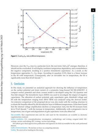
in terms of SS, ION/IOFF ratio and threshold voltage with respect to temperature. As shown,
the SS is much steeper at lower temperatures, while Vth and ION/IOFF are lower at higher
temperatures. Since SS = kT/q, it is clear that the SS increases with the increase in temperature. The
threshold voltage decreases with an increase in temperature showing the positive temperature
coefficient because of the changes in the Fermi level and bandgap [33]. The ION/IOFF ratio
achieves maximum value at lower temperatures, but the switching ratio of the NC-DG-JAM-FET
is still better than that of the DG-JAM-FET.
Figures 5 and 6 show the contour plots of the electron concentration and conduction band
energy at various temperatures for both the DG-JAM-FET and NC-DG-JAM-FET devices. It can
be interpreted that the conduction happens through the bulk of silicon in the NC-DG-JAM-FET,
due to which the depletion capacitance exists from the off-state to the on-state of the transistor.
This varying depletion capacitance offers effective capacitance matching and thus reduces the
major issue of hysteresis in FE-FETs [34].
(b) Analytical results showing the effects of temperature on the negative capacitance
double gate junctionless accumulation mode field effect transistor
The surface potential (φSP) variation with gate voltage (VGS) for a particular temperature (T)
range in figure 7a is directly calculated from equations (3.7) and (3.14). As is evident, the step-up
Downloaded
from
https://royalsocietypublishing.org/
on
01
March
2023

10. 10
royalsocietypublishing.org/journal/rspa
Proc.
R.
Soc.
A
479:
20220528
.
.
.
.
.
.
.
.
.
.
.
.
.
.
.
.
.
.
.
.
.
.
.
.
.
.
.
.
.
.
.
.
.
.
.
.
.
.
.
.
.
.
.
.
.
.
.
.
.
.
.
.
.
.
.
.
.
.
(b)
(a)
200 250 300
NC-DG-JAM-FET
DG-JAM-FET
NC-DG-JAM-FET
DG-JAM-FET
350
temperature (K)
400 450 500 200 250 300 350
temperature (K)
400 450 500
40 0.24
0.28
0.32
0.36
0.40
0.44
60
SS
(mV
dec
–1
)
80
100
1.5 × 1012
1.2 × 1012
9.0 × 1011
6.0 × 1011
3.0 × 1011
0
I
ON
/I
OFF
V
th
(V)
Figure 4. (a) SS and ION/IOFF ratio. (b) Threshold voltage of the devices with temperature variation.
5.60 × 1020
4.80 × 1020
4.00 × 1020
3.20 × 1020
2.40 × 1020
1.60 × 1020
8.00 × 1020
0
electron conc. (cm–3)
1.68 × 1020
1.44 × 1020
1.20 × 1020
9.60 × 1019
7.20 × 1019
4.80 × 1019
2.40 × 1019
0
electron conc. (cm–3)
T = 200 K
T = 200 K
T = 300 K
T = 300 K
T = 400 K
T = 400 K
T = 500 K
T = 500 K
(a)
(b)
Figure5. ContourplotforelectronconcentrationoftheDG-JAM-FET(a)andtheNC-DG-JAM-FET(b)atdifferenttemperatures.
conduction band energy (eV)
conduction band energy (eV)
3.3
2.7
2.1
1.5
0.9
0.3
–0.3
3.5
2.9
2.3
1.7
1.1
0.5
–0.1
T = 200 K
T = 200 K
T = 300 K
T = 300 K
T = 400 K
T = 400 K
T = 500 K
T = 500 K
(a)
(b)
Figure6. ContourplotforconductionbandenergyoftheDG-JAM-FET(a)andtheNC-DG-JAM-FET(b)atdifferenttemperatures.
conversion capacity of the NC-DG-JAM-FET gradually diminishes as the temperature rises.
This trend can also be seen in figure 7b. The voltage amplification factor or gain is defined in
equation (3.21). This property indicates that the negative capacitance effect diminishes with rising
temperature, which is consistent with experimental observations [35]. The ability to raise the
surface potential in this arrangement when the ferroelectric is in the negative capacitance area can
Downloaded
from
https://royalsocietypublishing.org/
on
01
March
2023

11. 11
royalsocietypublishing.org/journal/rspa
Proc.
R.
Soc.
A
479:
20220528
.
.
.
.
.
.
.
.
.
.
.
.
.
.
.
.
.
.
.
.
.
.
.
.
.
.
.
.
.
.
.
.
.
.
.
.
.
.
.
.
.
.
.
.
.
.
.
.
.
.
.
.
.
.
.
.
.
.
(a) (b) (c)
0.5 4 1.0
0.8
0.6
0.4
0.2
0
3
2
1
0
0.4
0.3
0.2
0.1
0
surface
potential
(V)
gain
gate
capacitance
(F
m
–2
)
–0.1
0 0.2 0.4 0.6 0.8 1.0
VGS (V)
0 0.2 0.4 0.6 0.8 1.0
VGS (V)
0 0.2 0.4 0.6 0.8 1.0
VGS (V)
T = 200 K
T = 300 K
T = 400 K
T = 500 K
T = 200 K
T = 300 K
T = 400 K
T = 500 K
T = 200 K
T = 300 K
T = 400 K
T = 500 K
Figure 7. Surface potential (a), gain (b), gate capacitance (c) as a function of VGS at various temperatures.
3.0
1800
1500
1200
900
600
300
0
0 0.2 0.4 0.6 0.8 1.0
0
2
4
6
8
10
12
2.5
2.0
1.5
1.0
0.5
0
0.8 1.0
0.6
0.4
0.2
0
VGS (V) VDS (V)
g
m
(mS)
g
d
(mS)
T = 200 K
T = 200 K
T = 400 K
T = 500 K
T = 200 K
T = 200 K
T = 400 K
T = 500 K
I
D
(A
m
–1
)
I
D
(A
m
–1
)
(a) (b)
10–14
10–12
10–10
10–8
10–6
10–4
Figure 8. Transfer characteristics and transconductance (a), output characteristics and output conductance (b) of the NC-DG-
JAM-FET at various temperatures.
be used to increase gate electrode control over a FET channel, yielding steeper SS that surpasses
the Boltzmann limit (SS 60 mV decade−1) [36].
We plotted the C–V characteristic curve of this structure at different temperatures in figure 7c
to study the temperature influence on gate capacitance in such devices. A significant gain is
indicated by the peaked C–V characteristic, which decreases as temperature increases. In other
words, when the temperature increases from 200 to 500 K, the NC impact continues to decrease.
The SS is generally stated by measuring the transfer characteristics curve. The ferroelectric
NC idea can explain values of SS 60 mV decade−1 at room temperature. Figure 8a shows the
input characteristics on the primary axis and transconductance on the secondary axis of our
investigated NC-DG-JAM-FET structure. Figure 8b shows the effects of temperature on the
output characteristics and output conductance of the proposed device when the gate voltage is
maintained at 1 V. As the temperature rises, the drain current decreases, leading to a fall in the
ION/IOFF ratio, as shown in the secondary axis of figure 9. This is how the phenomenon of the
temperature-dependent negative capacitance of drain current can be explained. The gate stack
capacitance (CG = Q/VGS) depends directly on the charge flowing across the channel while VGS is
constant.
The SS values increased from 46 to 72 mV decade−1 with the increase in temperature, as
is evident in the primary axis of figure 9. The dependency of SS on temperature is evident
from equation (3.23). On the other hand, when the temperature rises, the inverse of amplified
voltage grows. The definition of ferroelectric capacitance might help you understand this:
1/CFE = 2αtFE + 12βtFEQ2 [37]. When the temperature approaches Tc, the maximum value of
2αtFE, which overrides the negative capacitance, drops, causing the negative capacitance to grow.
Downloaded
from
https://royalsocietypublishing.org/
on
01
March
2023

12. 12
royalsocietypublishing.org/journal/rspa
Proc.
R.
Soc.
A
479:
20220528
.
.
.
.
.
.
.
.
.
.
.
.
.
.
.
.
.
.
.
.
.
.
.
.
.
.
.
.
.
.
.
.
.
.
.
.
.
.
.
.
.
.
.
.
.
.
.
.
.
.
.
.
.
.
.
.
.
.
2.6 × 107
2.4 × 107
2.2 × 107
2.0 × 107
1.8 × 107
I
ON
/I
OFF
1.6 × 107
1.4 × 107
1.2 × 107
8.0 × 106
500
450
400
350
temperature (K)
300
250
200
1.0 × 107
75
70
65
60
SS
(mV
dec
–1
)
55
50
45
Figure 9. SS and ION/IOFF ratio at different temperatures.
However, once the VGS rises to a particular level, the next term 12βtFEQ2 emerges; therefore, it
should not be overlooked. It will display nonlinear temperature dependency and counterbalance
the negative component, resulting in a positive ferroelectric capacitance. As a result, as the
temperature approaches Tc, CFE drops. According to equation (3.23), there is a linear increase
in the SS with temperature. Consequently, after an inevitable rise in temperature, the SS is
significantly more than 60 mV decade−1.
5. Conclusion
In this study, we presented an analytical approach for showing the influence of temperature
on the surface potential and drain current of a symmetric long-channel NC-DG-JAM-FET. A
compact surface potential and drain current model is developed using the L-K equation and
Pao–Sah integral. The ferroelectric layer (HZO) was used to investigate the impact of negative
capacitance. The alteration of surface potential, gate capacitance, gain, threshold voltage and
SS with the temperature ranging from 200 to 500 K was analysed using the derived model.
An extensive comparison of the proposed device was also made with the existing structure to
evaluate the benefits offered by the ferroelectric layer at different temperatures. It has been found
that the internal voltage amplification declines as temperature rises, but the SS increases from
46 to 72 mV decade−1 with the increase in temperature. Additionally, with a progressive rise in
temperature, loss of gain and degradation of gate capacitance were also observed.
Data accessibility. Raw experimental data and the code used for the simulations are available as electronic
supplementary material.
Authors’ contributions. S.Y.: conceptualization, investigation, methodology and writing—original draft; S.R.:
writing—review and editing; R.P.: writing—review and editing.
All authors gave final approval for publication and agreed to be held accountable for the work performed
therein.
Conflict of interest declaration. We declare we have no competing interests.
Funding. We received no funding for this study.
Downloaded
from
https://royalsocietypublishing.org/
on
01
March
2023

13. 13
royalsocietypublishing.org/journal/rspa
Proc.
R.
Soc.
A
479:
20220528
.
.
.
.
.
.
.
.
.
.
.
.
.
.
.
.
.
.
.
.
.
.
.
.
.
.
.
.
.
.
.
.
.
.
.
.
.
.
.
.
.
.
.
.
.
.
.
.
.
.
.
.
.
.
.
.
.
.
Appendix A
Table 1. Various symbols and their meanings.
symbols meaning
φ electrostatic channel potential of the device
. . . . . . . . . . . . . . . . . . . . . . . . . . . . . . . . . . . . . . . . . . . . . . . . . . . . . . . . . . . . . . . . . . . . . . . . . . . . . . . . . . . . . . . . . . . . . . . . . . . . . . . . . . . . . . . . . . . . . . . . . . . . . . . . . . . . . . . . . . . . . . . . . . . . . . . . . . . . . . . . . . . . . . . . . . . . . . . . . . . . . . . . . . . . . . . . . . . . . . . . . .
ND doping concentration in channel region
. . . . . . . . . . . . . . . . . . . . . . . . . . . . . . . . . . . . . . . . . . . . . . . . . . . . . . . . . . . . . . . . . . . . . . . . . . . . . . . . . . . . . . . . . . . . . . . . . . . . . . . . . . . . . . . . . . . . . . . . . . . . . . . . . . . . . . . . . . . . . . . . . . . . . . . . . . . . . . . . . . . . . . . . . . . . . . . . . . . . . . . . . . . . . . . . . . . . . . . . . .
εsi silicon permittivity
. . . . . . . . . . . . . . . . . . . . . . . . . . . . . . . . . . . . . . . . . . . . . . . . . . . . . . . . . . . . . . . . . . . . . . . . . . . . . . . . . . . . . . . . . . . . . . . . . . . . . . . . . . . . . . . . . . . . . . . . . . . . . . . . . . . . . . . . . . . . . . . . . . . . . . . . . . . . . . . . . . . . . . . . . . . . . . . . . . . . . . . . . . . . . . . . . . . . . . . . . .
εIL insulator/oxide permittivity
. . . . . . . . . . . . . . . . . . . . . . . . . . . . . . . . . . . . . . . . . . . . . . . . . . . . . . . . . . . . . . . . . . . . . . . . . . . . . . . . . . . . . . . . . . . . . . . . . . . . . . . . . . . . . . . . . . . . . . . . . . . . . . . . . . . . . . . . . . . . . . . . . . . . . . . . . . . . . . . . . . . . . . . . . . . . . . . . . . . . . . . . . . . . . . . . . . . . . . . . . .
q electronic charge
. . . . . . . . . . . . . . . . . . . . . . . . . . . . . . . . . . . . . . . . . . . . . . . . . . . . . . . . . . . . . . . . . . . . . . . . . . . . . . . . . . . . . . . . . . . . . . . . . . . . . . . . . . . . . . . . . . . . . . . . . . . . . . . . . . . . . . . . . . . . . . . . . . . . . . . . . . . . . . . . . . . . . . . . . . . . . . . . . . . . . . . . . . . . . . . . . . . . . . . . . .
V electron quasi-Fermi potential
. . . . . . . . . . . . . . . . . . . . . . . . . . . . . . . . . . . . . . . . . . . . . . . . . . . . . . . . . . . . . . . . . . . . . . . . . . . . . . . . . . . . . . . . . . . . . . . . . . . . . . . . . . . . . . . . . . . . . . . . . . . . . . . . . . . . . . . . . . . . . . . . . . . . . . . . . . . . . . . . . . . . . . . . . . . . . . . . . . . . . . . . . . . . . . . . . . . . . . . . . .
φSP surface potential: in simplest terms, it is the difference between the voltage at the surface of the MOSFET capacitor.
. . . . . . . . . . . . . . . . . . . . . . . . . . . . . . . . . . . . . . . . . . . . . . . . . . . . . . . . . . . . . . . . . . . . . . . . . . . . . . . . . . . . . . . . . . . . . . . . . . . . . . . . . . . . . . . . . . . . . . . . . . . . . . . . . . . . . . . . . . . . . . . . . . . . . . . . . . . . . . . . . . . . . . . . . . . . . . . . . . . . . . . . . . . . . . . . . . . . . . . . . .
φCP centre potential
. . . . . . . . . . . . . . . . . . . . . . . . . . . . . . . . . . . . . . . . . . . . . . . . . . . . . . . . . . . . . . . . . . . . . . . . . . . . . . . . . . . . . . . . . . . . . . . . . . . . . . . . . . . . . . . . . . . . . . . . . . . . . . . . . . . . . . . . . . . . . . . . . . . . . . . . . . . . . . . . . . . . . . . . . . . . . . . . . . . . . . . . . . . . . . . . . . . . . . . . . .
φM work function of metal
. . . . . . . . . . . . . . . . . . . . . . . . . . . . . . . . . . . . . . . . . . . . . . . . . . . . . . . . . . . . . . . . . . . . . . . . . . . . . . . . . . . . . . . . . . . . . . . . . . . . . . . . . . . . . . . . . . . . . . . . . . . . . . . . . . . . . . . . . . . . . . . . . . . . . . . . . . . . . . . . . . . . . . . . . . . . . . . . . . . . . . . . . . . . . . . . . . . . . . . . . .
φsi work function of semiconductor
. . . . . . . . . . . . . . . . . . . . . . . . . . . . . . . . . . . . . . . . . . . . . . . . . . . . . . . . . . . . . . . . . . . . . . . . . . . . . . . . . . . . . . . . . . . . . . . . . . . . . . . . . . . . . . . . . . . . . . . . . . . . . . . . . . . . . . . . . . . . . . . . . . . . . . . . . . . . . . . . . . . . . . . . . . . . . . . . . . . . . . . . . . . . . . . . . . . . . . . . . .
χ electron affinity
. . . . . . . . . . . . . . . . . . . . . . . . . . . . . . . . . . . . . . . . . . . . . . . . . . . . . . . . . . . . . . . . . . . . . . . . . . . . . . . . . . . . . . . . . . . . . . . . . . . . . . . . . . . . . . . . . . . . . . . . . . . . . . . . . . . . . . . . . . . . . . . . . . . . . . . . . . . . . . . . . . . . . . . . . . . . . . . . . . . . . . . . . . . . . . . . . . . . . . . . . .
Eg energy band gap
. . . . . . . . . . . . . . . . . . . . . . . . . . . . . . . . . . . . . . . . . . . . . . . . . . . . . . . . . . . . . . . . . . . . . . . . . . . . . . . . . . . . . . . . . . . . . . . . . . . . . . . . . . . . . . . . . . . . . . . . . . . . . . . . . . . . . . . . . . . . . . . . . . . . . . . . . . . . . . . . . . . . . . . . . . . . . . . . . . . . . . . . . . . . . . . . . . . . . . . . . .
ND
+
doping concentration in source/drain regions
. . . . . . . . . . . . . . . . . . . . . . . . . . . . . . . . . . . . . . . . . . . . . . . . . . . . . . . . . . . . . . . . . . . . . . . . . . . . . . . . . . . . . . . . . . . . . . . . . . . . . . . . . . . . . . . . . . . . . . . . . . . . . . . . . . . . . . . . . . . . . . . . . . . . . . . . . . . . . . . . . . . . . . . . . . . . . . . . . . . . . . . . . . . . . . . . . . . . . . . . . .
tCH thickness of the channel layer
. . . . . . . . . . . . . . . . . . . . . . . . . . . . . . . . . . . . . . . . . . . . . . . . . . . . . . . . . . . . . . . . . . . . . . . . . . . . . . . . . . . . . . . . . . . . . . . . . . . . . . . . . . . . . . . . . . . . . . . . . . . . . . . . . . . . . . . . . . . . . . . . . . . . . . . . . . . . . . . . . . . . . . . . . . . . . . . . . . . . . . . . . . . . . . . . . . . . . . . . . .
tFE thickness of the ferroelectric layer
. . . . . . . . . . . . . . . . . . . . . . . . . . . . . . . . . . . . . . . . . . . . . . . . . . . . . . . . . . . . . . . . . . . . . . . . . . . . . . . . . . . . . . . . . . . . . . . . . . . . . . . . . . . . . . . . . . . . . . . . . . . . . . . . . . . . . . . . . . . . . . . . . . . . . . . . . . . . . . . . . . . . . . . . . . . . . . . . . . . . . . . . . . . . . . . . . . . . . . . . . .
tIL thickness of the insulator layer
. . . . . . . . . . . . . . . . . . . . . . . . . . . . . . . . . . . . . . . . . . . . . . . . . . . . . . . . . . . . . . . . . . . . . . . . . . . . . . . . . . . . . . . . . . . . . . . . . . . . . . . . . . . . . . . . . . . . . . . . . . . . . . . . . . . . . . . . . . . . . . . . . . . . . . . . . . . . . . . . . . . . . . . . . . . . . . . . . . . . . . . . . . . . . . . . . . . . . . . . . .
QTOT total charge density over the entire channel (per unit gate area)
. . . . . . . . . . . . . . . . . . . . . . . . . . . . . . . . . . . . . . . . . . . . . . . . . . . . . . . . . . . . . . . . . . . . . . . . . . . . . . . . . . . . . . . . . . . . . . . . . . . . . . . . . . . . . . . . . . . . . . . . . . . . . . . . . . . . . . . . . . . . . . . . . . . . . . . . . . . . . . . . . . . . . . . . . . . . . . . . . . . . . . . . . . . . . . . . . . . . . . . . . .
VFE drop across ferroelectric layer
. . . . . . . . . . . . . . . . . . . . . . . . . . . . . . . . . . . . . . . . . . . . . . . . . . . . . . . . . . . . . . . . . . . . . . . . . . . . . . . . . . . . . . . . . . . . . . . . . . . . . . . . . . . . . . . . . . . . . . . . . . . . . . . . . . . . . . . . . . . . . . . . . . . . . . . . . . . . . . . . . . . . . . . . . . . . . . . . . . . . . . . . . . . . . . . . . . . . . . . . . .
VIL drop across insulator layer
. . . . . . . . . . . . . . . . . . . . . . . . . . . . . . . . . . . . . . . . . . . . . . . . . . . . . . . . . . . . . . . . . . . . . . . . . . . . . . . . . . . . . . . . . . . . . . . . . . . . . . . . . . . . . . . . . . . . . . . . . . . . . . . . . . . . . . . . . . . . . . . . . . . . . . . . . . . . . . . . . . . . . . . . . . . . . . . . . . . . . . . . . . . . . . . . . . . . . . . . . .
VFB flat-band voltage which results due to the difference in the work function of the metal and semiconductors
. . . . . . . . . . . . . . . . . . . . . . . . . . . . . . . . . . . . . . . . . . . . . . . . . . . . . . . . . . . . . . . . . . . . . . . . . . . . . . . . . . . . . . . . . . . . . . . . . . . . . . . . . . . . . . . . . . . . . . . . . . . . . . . . . . . . . . . . . . . . . . . . . . . . . . . . . . . . . . . . . . . . . . . . . . . . . . . . . . . . . . . . . . . . . . . . . . . . . . . . . .
Vth threshold voltage
. . . . . . . . . . . . . . . . . . . . . . . . . . . . . . . . . . . . . . . . . . . . . . . . . . . . . . . . . . . . . . . . . . . . . . . . . . . . . . . . . . . . . . . . . . . . . . . . . . . . . . . . . . . . . . . . . . . . . . . . . . . . . . . . . . . . . . . . . . . . . . . . . . . . . . . . . . . . . . . . . . . . . . . . . . . . . . . . . . . . . . . . . . . . . . . . . . . . . . . . . .
QMOB mobile charge density over the entire channel
. . . . . . . . . . . . . . . . . . . . . . . . . . . . . . . . . . . . . . . . . . . . . . . . . . . . . . . . . . . . . . . . . . . . . . . . . . . . . . . . . . . . . . . . . . . . . . . . . . . . . . . . . . . . . . . . . . . . . . . . . . . . . . . . . . . . . . . . . . . . . . . . . . . . . . . . . . . . . . . . . . . . . . . . . . . . . . . . . . . . . . . . . . . . . . . . . . . . . . . . . .
ID drain current
. . . . . . . . . . . . . . . . . . . . . . . . . . . . . . . . . . . . . . . . . . . . . . . . . . . . . . . . . . . . . . . . . . . . . . . . . . . . . . . . . . . . . . . . . . . . . . . . . . . . . . . . . . . . . . . . . . . . . . . . . . . . . . . . . . . . . . . . . . . . . . . . . . . . . . . . . . . . . . . . . . . . . . . . . . . . . . . . . . . . . . . . . . . . . . . . . . . . . . . . . .
VGS gate to source voltage
. . . . . . . . . . . . . . . . . . . . . . . . . . . . . . . . . . . . . . . . . . . . . . . . . . . . . . . . . . . . . . . . . . . . . . . . . . . . . . . . . . . . . . . . . . . . . . . . . . . . . . . . . . . . . . . . . . . . . . . . . . . . . . . . . . . . . . . . . . . . . . . . . . . . . . . . . . . . . . . . . . . . . . . . . . . . . . . . . . . . . . . . . . . . . . . . . . . . . . . . . .
k Boltzmann constant
. . . . . . . . . . . . . . . . . . . . . . . . . . . . . . . . . . . . . . . . . . . . . . . . . . . . . . . . . . . . . . . . . . . . . . . . . . . . . . . . . . . . . . . . . . . . . . . . . . . . . . . . . . . . . . . . . . . . . . . . . . . . . . . . . . . . . . . . . . . . . . . . . . . . . . . . . . . . . . . . . . . . . . . . . . . . . . . . . . . . . . . . . . . . . . . . . . . . . . . . . .
T temperature
. . . . . . . . . . . . . . . . . . . . . . . . . . . . . . . . . . . . . . . . . . . . . . . . . . . . . . . . . . . . . . . . . . . . . . . . . . . . . . . . . . . . . . . . . . . . . . . . . . . . . . . . . . . . . . . . . . . . . . . . . . . . . . . . . . . . . . . . . . . . . . . . . . . . . . . . . . . . . . . . . . . . . . . . . . . . . . . . . . . . . . . . . . . . . . . . . . . . . . . . . .
Tc Curie temperature
. . . . . . . . . . . . . . . . . . . . . . . . . . . . . . . . . . . . . . . . . . . . . . . . . . . . . . . . . . . . . . . . . . . . . . . . . . . . . . . . . . . . . . . . . . . . . . . . . . . . . . . . . . . . . . . . . . . . . . . . . . . . . . . . . . . . . . . . . . . . . . . . . . . . . . . . . . . . . . . . . . . . . . . . . . . . . . . . . . . . . . . . . . . . . . . . . . . . . . . . . .
CTOT total gate capacitance
. . . . . . . . . . . . . . . . . . . . . . . . . . . . . . . . . . . . . . . . . . . . . . . . . . . . . . . . . . . . . . . . . . . . . . . . . . . . . . . . . . . . . . . . . . . . . . . . . . . . . . . . . . . . . . . . . . . . . . . . . . . . . . . . . . . . . . . . . . . . . . . . . . . . . . . . . . . . . . . . . . . . . . . . . . . . . . . . . . . . . . . . . . . . . . . . . . . . . . . . . .
CIL capacitance across insulator layer
. . . . . . . . . . . . . . . . . . . . . . . . . . . . . . . . . . . . . . . . . . . . . . . . . . . . . . . . . . . . . . . . . . . . . . . . . . . . . . . . . . . . . . . . . . . . . . . . . . . . . . . . . . . . . . . . . . . . . . . . . . . . . . . . . . . . . . . . . . . . . . . . . . . . . . . . . . . . . . . . . . . . . . . . . . . . . . . . . . . . . . . . . . . . . . . . . . . . . . . . . .
CS semiconductor capacitance
. . . . . . . . . . . . . . . . . . . . . . . . . . . . . . . . . . . . . . . . . . . . . . . . . . . . . . . . . . . . . . . . . . . . . . . . . . . . . . . . . . . . . . . . . . . . . . . . . . . . . . . . . . . . . . . . . . . . . . . . . . . . . . . . . . . . . . . . . . . . . . . . . . . . . . . . . . . . . . . . . . . . . . . . . . . . . . . . . . . . . . . . . . . . . . . . . . . . . . . . . .
CFE ferroelectric capacitance
. . . . . . . . . . . . . . . . . . . . . . . . . . . . . . . . . . . . . . . . . . . . . . . . . . . . . . . . . . . . . . . . . . . . . . . . . . . . . . . . . . . . . . . . . . . . . . . . . . . . . . . . . . . . . . . . . . . . . . . . . . . . . . . . . . . . . . . . . . . . . . . . . . . . . . . . . . . . . . . . . . . . . . . . . . . . . . . . . . . . . . . . . . . . . . . . . . . . . . . . . .
CG gate stack capacitance
. . . . . . . . . . . . . . . . . . . . . . . . . . . . . . . . . . . . . . . . . . . . . . . . . . . . . . . . . . . . . . . . . . . . . . . . . . . . . . . . . . . . . . . . . . . . . . . . . . . . . . . . . . . . . . . . . . . . . . . . . . . . . . . . . . . . . . . . . . . . . . . . . . . . . . . . . . . . . . . . . . . . . . . . . . . . . . . . . . . . . . . . . . . . . . . . . . . . . . . . . .
Q surface charge
. . . . . . . . . . . . . . . . . . . . . . . . . . . . . . . . . . . . . . . . . . . . . . . . . . . . . . . . . . . . . . . . . . . . . . . . . . . . . . . . . . . . . . . . . . . . . . . . . . . . . . . . . . . . . . . . . . . . . . . . . . . . . . . . . . . . . . . . . . . . . . . . . . . . . . . . . . . . . . . . . . . . . . . . . . . . . . . . . . . . . . . . . . . . . . . . . . . . . . . . . .
α,β,γ the Landau-coefficients that depend on the ferroelectric material properties typical of HZO
. . . . . . . . . . . . . . . . . . . . . . . . . . . . . . . . . . . . . . . . . . . . . . . . . . . . . . . . . . . . . . . . . . . . . . . . . . . . . . . . . . . . . . . . . . . . . . . . . . . . . . . . . . . . . . . . . . . . . . . . . . . . . . . . . . . . . . . . . . . . . . . . . . . . . . . . . . . . . . . . . . . . . . . . . . . . . . . . . . . . . . . . . . . . . . . . . . . . . . . . . .
gm transconductance
. . . . . . . . . . . . . . . . . . . . . . . . . . . . . . . . . . . . . . . . . . . . . . . . . . . . . . . . . . . . . . . . . . . . . . . . . . . . . . . . . . . . . . . . . . . . . . . . . . . . . . . . . . . . . . . . . . . . . . . . . . . . . . . . . . . . . . . . . . . . . . . . . . . . . . . . . . . . . . . . . . . . . . . . . . . . . . . . . . . . . . . . . . . . . . . . . . . . . . . . . .
(Continued.)
Downloaded
from
https://royalsocietypublishing.org/
on
01
March
2023

14. 14
royalsocietypublishing.org/journal/rspa
Proc.
R.
Soc.
A
479:
20220528
.
.
.
.
.
.
.
.
.
.
.
.
.
.
.
.
.
.
.
.
.
.
.
.
.
.
.
.
.
.
.
.
.
.
.
.
.
.
.
.
.
.
.
.
.
.
.
.
.
.
.
.
.
.
.
.
.
.
Table 1. (Continued.)
symbols meaning
. . . . . . . . . . . . . . . . . . . . . . . . . . . . . . . . . . . . . . . . . . . . . . . . . . . . . . . . . . . . . . . . . . . . . . . . . . . . . . . . . . . . . . . . . . . . . . . . . . . . . . . . . . . . . . . . . . . . . . . . . . . . . . . . . . . . . . . . . . . . . . . . . . . . . . . . . . . . . . . . . . . . . . . . . . . . . . . . . . . . . . . . . . . . . . . . . . . . . . . . . .
W/L width to length ratio of the transistor
. . . . . . . . . . . . . . . . . . . . . . . . . . . . . . . . . . . . . . . . . . . . . . . . . . . . . . . . . . . . . . . . . . . . . . . . . . . . . . . . . . . . . . . . . . . . . . . . . . . . . . . . . . . . . . . . . . . . . . . . . . . . . . . . . . . . . . . . . . . . . . . . . . . . . . . . . . . . . . . . . . . . . . . . . . . . . . . . . . . . . . . . . . . . . . . . . . . . . . . . . .
μ mobility of the charge carrier
. . . . . . . . . . . . . . . . . . . . . . . . . . . . . . . . . . . . . . . . . . . . . . . . . . . . . . . . . . . . . . . . . . . . . . . . . . . . . . . . . . . . . . . . . . . . . . . . . . . . . . . . . . . . . . . . . . . . . . . . . . . . . . . . . . . . . . . . . . . . . . . . . . . . . . . . . . . . . . . . . . . . . . . . . . . . . . . . . . . . . . . . . . . . . . . . . . . . . . . . . .
U ferroelectric’s free energy density
. . . . . . . . . . . . . . . . . . . . . . . . . . . . . . . . . . . . . . . . . . . . . . . . . . . . . . . . . . . . . . . . . . . . . . . . . . . . . . . . . . . . . . . . . . . . . . . . . . . . . . . . . . . . . . . . . . . . . . . . . . . . . . . . . . . . . . . . . . . . . . . . . . . . . . . . . . . . . . . . . . . . . . . . . . . . . . . . . . . . . . . . . . . . . . . . . . . . . . . . . .
E external applied electric field
. . . . . . . . . . . . . . . . . . . . . . . . . . . . . . . . . . . . . . . . . . . . . . . . . . . . . . . . . . . . . . . . . . . . . . . . . . . . . . . . . . . . . . . . . . . . . . . . . . . . . . . . . . . . . . . . . . . . . . . . . . . . . . . . . . . . . . . . . . . . . . . . . . . . . . . . . . . . . . . . . . . . . . . . . . . . . . . . . . . . . . . . . . . . . . . . . . . . . . . . . .
P polarization
. . . . . . . . . . . . . . . . . . . . . . . . . . . . . . . . . . . . . . . . . . . . . . . . . . . . . . . . . . . . . . . . . . . . . . . . . . . . . . . . . . . . . . . . . . . . . . . . . . . . . . . . . . . . . . . . . . . . . . . . . . . . . . . . . . . . . . . . . . . . . . . . . . . . . . . . . . . . . . . . . . . . . . . . . . . . . . . . . . . . . . . . . . . . . . . . . . . . . . . . . .
References
1. Alam MA, Si M, Ye PD. 2019 A critical review of recent progress on negative capacitance
field-effect transistors. Appl. Phys. Lett. 114, 090401. (doi:10.1063/1.5092684)
2. Salahuddin S. 2016 Review of negative capacitance transistors. In International Symposium
on VLSI Technology, Systems and Application (VLSI-TSA), Hsinchu, Taiwan, 1-1. IEEE.
(doi:10.1109/VLSI-TSA.2016.7480491)
3. Lin CI, Khan AI, Salahuddin S, Hu C. 2016 Effects of the variation of ferroelectric properties
on negative capacitance FET characteristics. IEEE Trans. Electron Devices 63, 2197–2199.
(doi:10.1109/TED.2016.2514783)
4. Mehta H, Kaur H. 2020 Superior performance and reliability of double gate Gaussian doped
negative capacitance junctionless transistor for 200–500K. IETE Tech. Rev. (Institution Electron.
Telecommun. Eng. India) 37, 391–401. (doi:10.1080/02564602.2019.1642149)
5. Kim TK et al. 2013 First demonstration of junctionless accumulation-mode bulk FinFETs
with robust junction isolation. IEEE Electron Device Lett. 34, 1479–1481. (doi:10.1109/
LED.2013.2283291)
6. Hun Choi J, Kyun Kim TK, Member S, Min Moon J, Gwang Yoon Y, Woon Hwang B,
Hyun Kim D, Lee SH. 2014 Origin of device performance enhancement of junctionless
accumulation-mode (JAM) bulk FinFETs with high-κ gate spacers. IEEE Electron Device Lett.
35, 1182–1184. (doi:10.1109/LED.2014.2364093)
7. Neshatpour K, Burleson W, Khajeh A, Homayoun H. 2018 Enhancing power, performance,
and energy efficiency in chip multiprocessors exploiting inverse thermal dependence. IEEE
Trans. Very Large Scale Integr. Syst. 26, 778–791. (doi:10.1109/TVLSI.2017.2780800)
8. Jo J, Shin C. 2015 Impact of temperature on negative capacitance field-effect transistor.
Electron. Lett. 51, 106–108. (doi:10.1049/el.2014.3515)
9. Saha AK, Gupta SK. 2020 Multi-domain negative capacitance effects in metal-ferroelectric-
insulator-semiconductor/metal stacks: a phase-field simulation based study. Sci. Rep. 10,
10207. (doi:10.1038/s41598-020-66313-1)
10. Müller J, Böscke TS, Schröder U, Mueller S, Bräuhaus D, Böttger U, Frey L, Mikolajick T.
2012 Ferroelectricity in simple binary ZrO2 and HfO2. Nano Lett. 12, 4318–4323. (doi:10.1021/
nl302049k)
11. Tsai MJ, Chen PJ, Ruan DB, Hou FJ, Peng PY, Chen LG, Wu YC. 2019 Investigation of 5-
nm-thick Hf0.5Zr0.5O2 ferroelectric FinFET dimensions for sub-60-mV/decade subthreshold
slope. IEEE J. Electron Devices Soc. 7, 1033–1037. (doi:10.1109/JEDS.2019.2942381)
12. Mulaosmanovic H, Breyer ET, Dünkel S, Beyer S, Mikolajick T, Slesazeck S. 2021
Ferroelectric field-effect transistors based on HfO2: a review. Nanotechnology 32, 502002.
(doi:10.1088/1361-6528/AC189F)
13. Singh B, Gola D, Singh K, Goel E, Kumar S, Jit S. 2017 Analytical modeling of subthreshold
characteristics of ion-implanted symmetric double gate junctionless field effect transistors.
Mater. Sci. Semicond. Process. 58, 82–88. (doi:10.1016/j.mssp.2016.10.051)
14. Atlas User Manual. 2019 A device simulation software package. Santa Clara, CA: Silvaco Int.
(https://silvaco.com/tcad/).
15. Hoffmann M, Slesazeck S, Mikolajick T. 2021 Progress and future prospects of negative
capacitance electronics: a materials perspective. APL Mater. 9, 20902. (doi:10.1063/5.0032954)
16. Liu Y, Li J. 2019 Seeing is believing: negative capacitance captured at both nano- and macro-
scales. Sci. Bull. 64, 361–363. (doi:10.1016/j.scib.2019.02.020)
Downloaded
from
https://royalsocietypublishing.org/
on
01
March
2023

15. 15
royalsocietypublishing.org/journal/rspa
Proc.
R.
Soc.
A
479:
20220528
.
.
.
.
.
.
.
.
.
.
.
.
.
.
.
.
.
.
.
.
.
.
.
.
.
.
.
.
.
.
.
.
.
.
.
.
.
.
.
.
.
.
.
.
.
.
.
.
.
.
.
.
.
.
.
.
.
.
17. Khan AI. 2019 On the microscopic origin of negative capacitance in ferroelectric materials: a
toy model. Tech. Dig. Int. Electron Devices Meet. IEDM 9.3.1–9.3.4.
18. Seo M et al. 2018 First demonstration of a logic-process compatible junctionless ferroelectric
FinFET synapse for neuromorphic applications. IEEE Electron Device Lett. 39, 1445–1448.
(doi:10.1109/LED.2018.2852698)
19. Najmzadeh M, Bouvet D, Grabinski W, Sallese JM, Ionescu AM. 2012 Accumulation-mode
gate-all-around si nanowire nMOSFETs with sub-5 nm cross-section and high uniaxial tensile
strain. Solid State Electron. 74, 114–120. (doi:10.1016/j.sse.2012.04.021)
20. Kwon D, Cheema S, Shanker N, Chatterjee K, Liao YH, Tan AJ, Hu C, Salahuddin S. 2019
Negative capacitance FET with 1.8-nm-thick Zr-doped HfO2 oxide. IEEE Electron Device Lett.
40, 993–996. (doi:10.1109/LED.2019.2912413)
21. Kim CK, Yang ES. 1970 On the validity of the gradual-channel approximation for field effect
transistors. Proceedings of the IEEE. 58, 841–842. (doi:10.1109/PROC.1970.7778)
22. Pao HC. 1966 Effects of diffusion current on characteristics of metal-oxide (insulator)-
semiconductor transistors. Solid. State. Electron. 9, 927–937.
23. Duarte JP, Choi SJ, Choi YK. 2011 A full-range drain current model for double-
gate junctionless transistors. IEEE Trans. Electron Devices 58, 4219–4225. (doi:10.1109/
TED.2011.2169266)
24. Peng Y, Han G, Chen Z, Li Q, Zhang J, Hao Y. 2018 Analytical calculation of influence of
ferroelectric properties on electrical characteristics negative capacitance germanium FETs.
IEEE J. Electron Devices Soc. 6, 233–239. (doi:10.1109/JEDS.2018.2794069)
25. Holtij T, Graef M, Hain FM, Kloes A, Iniguez B. 2014 Compact model for short-channel
junctionless accumulation mode double gate MOSFETs. IEEE Trans. Electron Devices 61,
288–299. (doi:10.1109/TED.2013.2281615)
26. He J, Liu F, Zhou XY, Zhang J, Zhang LN. 2011 A continuous analytic channel potential
solution to doped symmetric double-gate MOSFETs from the accumulation to the strong-
inversion region. Chinese Phys. B 20, 1–6. (doi:10.1088/1674-1056/20/1/016102)
27. Mehta H, Kaur H. 2016 Modeling and simulation study of novel Double Gate Ferroelectric
Junctionless (DGFJL) transistor. Superlattices Microstruct. 97, 536–547. (doi:10.1016/
j.spmi.2016.07.024)
28. Salahuddin S, Datta S. 2008 Use of negative capacitance to provide voltage amplification for
low power nanoscale devices. Nano Lett. 8, 405–410. (doi:10.1021/nl071804g)
29. Hoffmann M, Max B, Mittmann T, Schroeder U, Slesazeck S, Mikolajick T. 2019
Demonstration of High-speed Hysteresis-free Negative Capacitance in Ferroelectric
Hf0.5Zr0.5O2. IEEE International Electron Devices Meeting (IEDM), San Francisco, CA, 31.6.1–
31.6.4. (doi:10.1109/IEDM.2018.8614677)
30. Pahwa G, Dutta T, Agarwal A, Khandelwal S, Salahuddin S, Hu C, Chauhan YS. 2016 Analysis
and compact modeling of negative capacitance transistor with high on-current and negative
output differential resistance - Part II: model validation. IEEE Trans. Electron Devices 63,
4986–4992. (doi:10.1109/TED.2016.2614436)
31. Lee H, Yoon Y, Shin C. 2017 Current-voltage model for negative capacitance field-effect
transistors. IEEE Electron Device Lett. 38, 669–672. (doi:10.1109/LED.2017.2679102)
32. Kim Y et al. 2021 Analytical current–voltage modeling and analysis of the mfis gate-all-around
transistor featuring negative-capacitance. Electron 10, 1177. (doi:10.3390/electronics10101177)
33. Pandey P, Kaur H. 2020 Improved temperature resilience and device performance of negative
capacitance reconfigurable field effect transistors. IEEE Trans. Electron Devices 67, 738–744.
(doi:10.1109/TED.2019.2961876)
34. Kumar M, Aditya K, Dixit A. 2020 A junctionless accumulation mode NC-FinFET gate
underlap design for improved stability and self-heating reduction. IEEE Trans. Electron Devices
67, 3424–3430. (doi:10.1109/TED.2020.2997848)
35. Salvatore GA, Rusu A, Ionescu AM. 2012 Experimental confirmation of temperature
dependent negative capacitance in ferroelectric field effect transistor. Appl. Phys. Lett. 100,
163504. (doi:10.1063/1.4704179)
36. Wang C, Wu J, Yu H, Han G, Miao X, Wang X. 2020 Effects of Temperature on the performance
of Hf0.5Zr0.5O2-based negative capacitance FETs. IEEE Electron Device Lett. 41, 1625–1628.
(doi:10.1109/LED.2020.3022384)
37. Kanithan S, Vignesh NA, Jana S, Prasad CG, Konguvel E, Vimalnath S. 2022 Negative
capacitance ferroelectric FET based on short channel effect for low power applications. Silicon
14, 9569–9579. (doi:10.1007/s12633-021-01625-z)
Downloaded
from
https://royalsocietypublishing.org/
on
01
March
2023