John and Betty Smith, aged 60 and 58 respectively, have 4 children and 9 grandchildren. They recently sold their business and are looking to retire. They have $6 million in total assets including $5 million in investments. Their annual expenses total $280,000. They want to ensure a financially secure retirement while funding their grandchildren's education and other goals. A proposed asset allocation of 60% stocks and 40% bonds is projected to meet their needs with an 8.3% expected annual return.

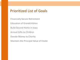
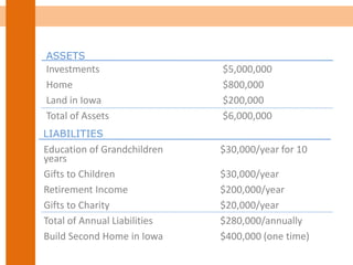
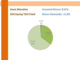
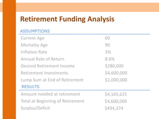
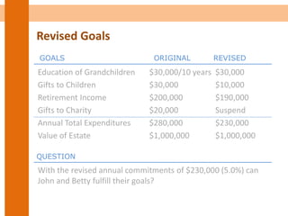
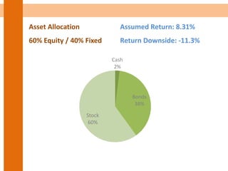
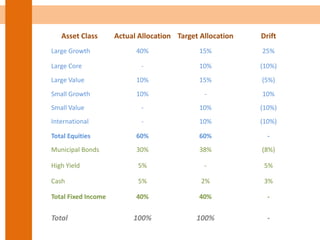
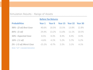
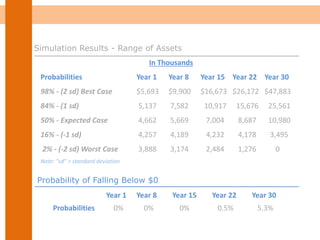
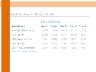
1. Wealth Management
Case Study– John & Betty Smith

2. John & Betty Smith
John and Betty recently
completed the sale of their
business and are looking
forward to a long and fulfilling
retirement.
JOHN
(AGE 60)
BETTY
(AGE 58)
4 CHILDREN
9 GRANDCHILDREN
Example

3. Prioritized List of Goals
Financially Secure Retirement
Education of Grandchildren
Build Second Home in Iowa
Annual Gifts to Children
Donate Money to Charity
Maintain the Principal Value of Estate

4. Investments $5,000,000
Home $800,000
Land in Iowa $200,000
Total of Assets $6,000,000
ASSETS
LIABILITIES
Education of Grandchildren $30,000/year for 10
years
Gifts to Children $30,000/year
Retirement Income $200,000/year
Gifts to Charity $20,000/year
Total of Annual Liabilities $280,000/annually
Build Second Home in Iowa $400,000 (one time)

5. Investment Assets $4,600,000
PRODUCTIVE ASSETS
USE ASSETS
Home $800,000
Land in Iowa $200,000
Set Aside for Second Home $400,000
LIABILITIES
Their annual commitments total $280,000 or approximately 6.1%
of their investment assets
QUESTION
With $4,600,000, can the Smith’s afford to fulfill their goals?

6. Hierarchy of Investment Priorities
High Returns - Growth
Low Volatility of Account
Consistency of Returns
Asset Growth
Fees (Lowest Possible)
Preservation of Income
Out Performing the Market
Finding Great Stock
Buying Hot Fund
Studying Economic Activities
Employing Market Timing Strategies
Finding Opportunities in the Markets
Understanding Your Investment Process
Making All Investment Decision
Not Running Out Of Money
Hedge Funds
Direct Real Estate
Venture Capital
Finding Highest Performing Money Manager

7. High Returns - Growth
Low Volatility of Account
Consistency of Returns
Asset Growth
Fees (Lowest Possible)
Preservation of Income
Out Performing the Market
Finding Great Stock
Buying Hot Fund
Studying Economic Activities
Employing Market Timing Strategies
Finding Opportunities in the Markets
Understanding Your Investment Process
Making All Investment Decision
Not Running Out Of Money
Hedge Funds
Direct Real Estate
Venture Capital
Finding Highest Performing Money Manager
Hierarchy of Investment Priorities
1
3
5
4
2

8. Asset Allocation? Assumed Return?

9. Asset Allocation Assumed Return: 8.61%
65% Equity/ 35% Fixed Return Downside: -11.8%
Cash
2%
Bonds
33%
Stock
65%

10. Retirement Funding Analysis
Current Age
Mortality Age
Inflation Rate
Annual Rate of Return
Desired Retirement Income
Retirement Investments
Lump Sum at End of Retirement
ASSUMPTIONS
60
90
3%
8.6%
$280,000
$4,600,000
$1,000,000
RESULTS
Amount needed at retirement
Total at Beginning of Retirement
Surplus/Deficit
$4,105,625
$4,600,000
$494,374

11. Probability of Falling Below $0
Year 1 Year 8 Year 15 Year 22 Year 30
Probabilities 0% 0% 0% 13.2% 37.1%
Note: “SD” = Standard Deviation
In Thousands
Probabilities Year 1 Year 8 Year 15 Year 22 Year 30
98% - (2 sd) Best Case $5,767 $9,552 $15,075 $22,462 $37,724
84% - (1 sd) 5,152 6,859 8,835 11,282 16,458
50% - Expected Case 4,660 4,830 4,863 4,591 3,135
16% - (-1 sd) 4,209 3,358 2,372 359 0
2% - (-2 sd) Worst Case 3,851 2,396 668 0 0
Note: "sd" = standard deviation
Simulation Results - Range of Assets

12. Asset Allocation Assumed Return: 9.51%
80% Equity / 20% Fixed Return Downside: -13.3%
Cash
2%
Bonds
18%
Stock
80%

13. Year 1 Year 8 Year 15 Year 22 Year 30
Probabilities 0% 0% 0% 11.5% 32.5%
In Thousands
Probabilities Year 1 Year 8 Year 15 Year 22 Year 30
98% - (2 sd) Best Case $6,101 $11,353 $22,985 $38,267 $57,470
84% - (1 sd) 5,293 7,308 10,775 15,835 27,269
50% - Expected Case 4,721 5,084 5,704 6,048 6,075
16% - (-1 sd) 4,102 3,239 2,572 902 0
2% - (-2 sd) Worst Case 3,737 2,303 312 0 0
Note: "sd" = standard deviation
Simulation Results - Range of Assets
Probability of Falling Below $0

14. Revised Goals
Education of Grandchildren
Gifts to Children
Retirement Income
Gifts to Charity
Annual Total Expenditures
Value of Estate
REVISEDORIGINALGOALS
QUESTION
With the revised annual commitments of $230,000 (5.0%) can
John and Betty fulfill their goals?
$30,000/10 years
$30,000
$200,000
$20,000
$280,000
$1,000,000
$30,000
$10,000
$190,000
Suspend
$230,000
$1,000,000

15. Asset Allocation Assumed Return: 8.31%
60% Equity / 40% Fixed Return Downside: -11.3%
Cash
2%
Bonds
38%
Stock
60%

16. Year 1 Year 8 Year 15 Year 22 Year 30
Probabilities 0% 0% 0% 0.5% 5.3%
In Thousands
Probabilities Year 1 Year 8 Year 15 Year 22 Year 30
98% - (2 sd) Best Case $5,693 $9,900 $16,673 $26,172 $47,883
84% - (1 sd) 5,137 7,582 10,917 15,676 25,561
50% - Expected Case 4,662 5,669 7,004 8,687 10,980
16% - (-1 sd) 4,257 4,189 4,232 4,178 3,495
2% - (-2 sd) Worst Case 3,888 3,174 2,484 1,276 0
Note: "sd" = standard deviation
Simulation Results - Range of Assets
Probability of Falling Below $0

17. Cash
5%
Muni Bonds
30%
High Yield
5%
Large
Growth
40%
Large Value
10%
Small
Growth
10%
Asset Allocation - Current Assumed Return: 8.76%
60% Equity / 40% Fixed Return Downside: -11.3%

18. Asset Class Actual Allocation Target Allocation Drift
Large Growth 40% 15% 25%
Large Core - 10% (10%)
Large Value 10% 15% (5%)
Small Growth 10% - 10%
Small Value - 10% (10%)
International - 10% (10%)
Total Equities 60% 60% -
Municipal Bonds 30% 38% (8%)
High Yield 5% - 5%
Cash 5% 2% 3%
Total Fixed Income 40% 40% -
Total 100% 100% -

19. In Thousands
Probabilities Year 1 Year 8 Year 15 Year 22 Year 30
98% - (2 sd) Best Case $5,884 $11,143 $18,711 $32,337 $60,658
84% - (1 sd) 5,209 7,975 11,801 17,245 29,891
50% - Expected Case 4,679 5,600 7,070 8,905 11,632
16% - (-1 sd) 4,188 3,988 3,985 3,577 2,790
2% - (-2 sd) Worst Case 3,801 2,891 1,918 583 0
Note: "sd" = standard deviation
Year 1 Year 8 Year 15 Year 22 Year 30
Probabilities 0% 0% 0% 1.1% 8.1%
Simulation Results - Range of Assets
Probability of Falling Below $0

20. Before-Tax Returns
Probabilities Year 1 Year 8 Year 15 Year 22 Year 30
98% - (2 sd) Best Case 40.6% 18.5% 15.5% 13.8% 12.8%
84% - (1 sd) 24.4% 13.2% 11.8% 11.1% 10.5%
50% - Expected Case 8.5% 8.3% 8.4% 8.4% 8.4%
16% - (-1 sd) -4.6% 4.1% 5.2% 5.7% 6.2%
2% - (-2 sd) Worst Case -15.2% -0.7% 2.2% 3.1% 4.1%
Note: "sd" = standard deviation
Simulation Results - Range of Assets

21. Cash
2%
Muni Bonds
38%
Large
Growth
15%Large Core
10%
Large Value
15%
Small Value
10%
Int'l Growth
5%
Int'l Value
5%
Asset Allocation - Proposed Assumed Return: 8.31%
60% Equity/ 40% Fixed Return Downside: -10.5%

22. Asset Class Actual Allocation Target Allocation Drift
Large Growth 15% 15% -
Large Core 10% 10% -
Large Value 15% 15% -
Small Growth 10% - 10%
Small Value 5% 10% (5%)
International 5% 10% (5%)
Total Equities 60% 60% -
Municipal Bonds 38% 38% -
Cash 2% 2% -
Total Fixed Income 40% 40% -
Total 100% 100% -

23. In Thousands
Probabilities Year 1 Year 8 Year 15 Year 22 Year 30
98% - (2 sd) Best Case $5,693 $9,900 $16,673 $26,172 $47,883
84% - (1 sd) 5,137 7,582 10,917 15,676 25,561
50% - Expected Case 4,662 5,669 7,004 8,687 10,980
16% - (-1 sd) 4,257 4,189 4,232 4,178 3,495
2% - (-2 sd) Worst Case 3,888 3,174 2,484 1,276 0
Note: "sd" = standard deviation
Year 1 Year 8 Year 15 Year 22 Year 30
Probabilities 0% 0% 0% 0.5% 5.3%
Simulation Results - Range of Assets
Probability of Falling Below $0

24. Before-Tax Returns
Probabilities Year 1 Year 8 Year 15 Year 22 Year 30
98% - (2 sd) Best Case 34.5% 16.8% 14.1% 13.0% 12.5%
84% - (1 sd) 21.5% 12.5% 11.4% 10.8% 10.5%
50% - Expected Case 8.5% 8.8% 8.7% 8.7% 8.6%
16% - (-1 sd) -2.5% 5.2% 6.0% 6.4% 6.8%
2% - (-2 sd) Worst Case -11.7% 1.5% 3.6% 4.2% 4.8%
Note: "sd" = standard deviation
Simulation Results - Range of Assets