Download as PDF, PPTX
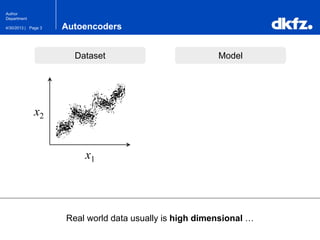
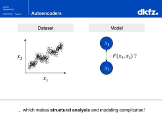
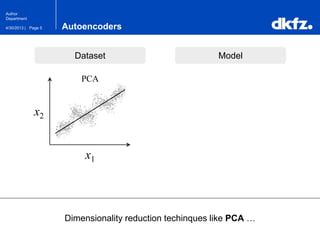
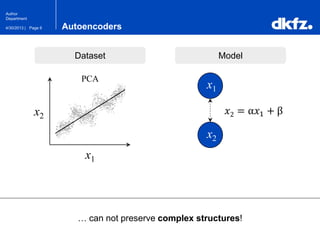
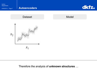
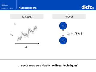
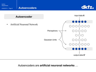
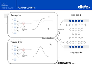

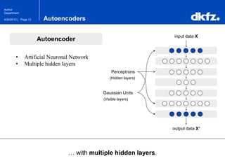
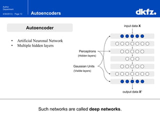
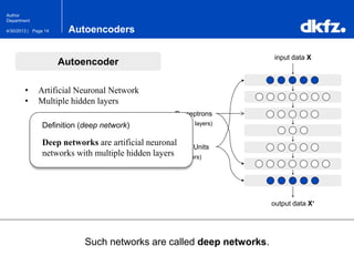


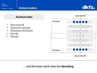
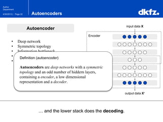
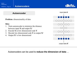
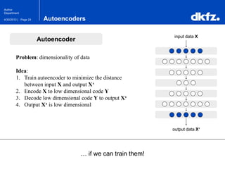

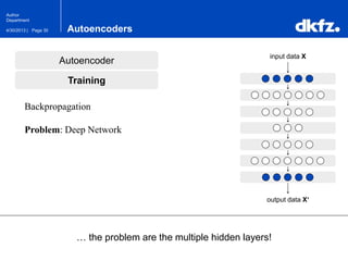

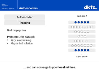
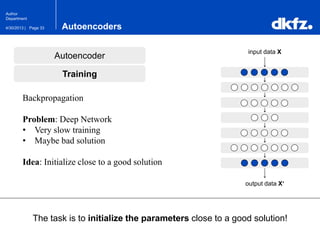
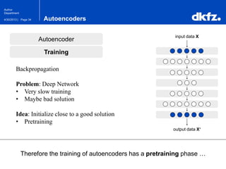
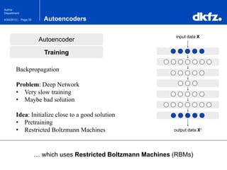
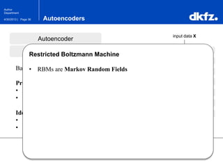
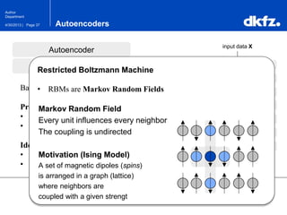
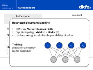

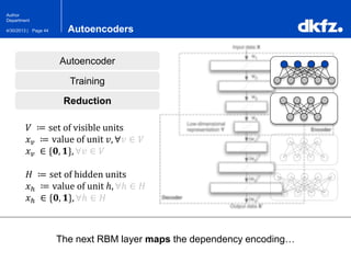
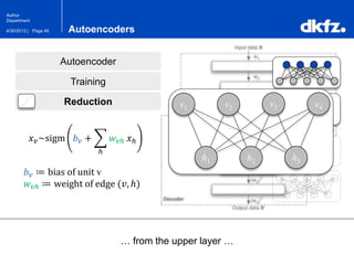

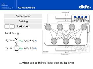
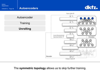
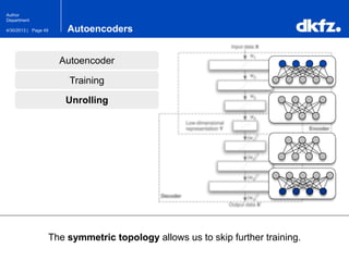
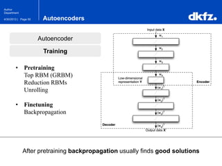
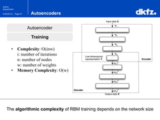


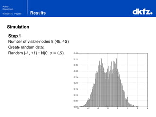
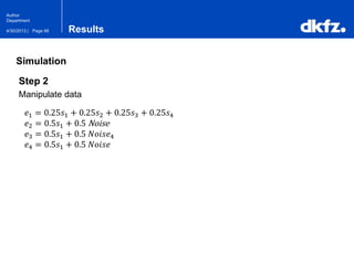
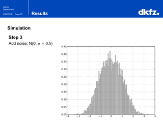
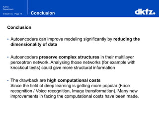

The document discusses the use of deep autoencoders for structural learning and modeling, emphasizing their ability to handle high-dimensional data through dimensionality reduction techniques. It outlines the architecture of autoencoders, including the encoding and decoding processes, and the importance of pretraining with Restricted Boltzmann Machines (RBMs) to improve training efficiency. The document also presents results related to the validation and implementation of autoencoders using artificial datasets to assess performance.