2. P. Sterlini et al.
1 3
linked to the NAO, especially during winter (Tsimplis and
Shaw 2008). Atmospheric forcing, in terms of barotropic
wind and pressure effects, has been shown to be a dominant
forcing factor (Wakelin et al. 2003; Woolf et al. 2003; Yan
et al. 2004). However, these barotropic influences seem to
diminish after a few years (Dangendorf et al. 2013). On
longer timescales baroclinic adjustment processes become
more important (Chen et al. 2014). Recent studies, for
instance, suggest that on longer timescales there is a large-
scale coherent response of the coastal waters to longshore
winds in the form of propagating boundary waves in the
NEA (Sturges and Douglas 2011; Calafat et al. 2012, 2013;
Dangendorf et al. 2014a). Changes in ocean heat content
also influence regional SSV (Bilbao et al. 2015) as it leads
to expansion or contraction of the water column, affects
ocean circulation and density patterns as well as the melt-
ing of (land) ice (Gornitz et al. 1982).
Much work investigating the mean sea level and SSV in
the North Sea has used tide gauge data as data records span
several decades and in some cases centuries (e.g. Yan et al.
2004; Woodworth et al. 2010; Calafat et al. 2012, 2013;
Richter et al. 2012; Calafat and Chambers 2013; Dan-
gendorf et al. 2014a). Tide gauge studies have provided a
wealth of detailed information relating to SSV at specific
stations which are usually situated coastally and inher-
ently limited in spatial coverage. A further limitation of tide
gauge data however is that they are not a priori representa-
tive of open ocean processes or mechanisms that affect SSH
from a remote location. Supplementary data sets such as
altimetry, steric heights from models or assumptions from
consistency between tide gauge locations have been used
to augment tide gauge data in order to connect them to the
spatial scale and make assumptions relating to processes
that operate over a spatial domain (Chambers et al. 2002;
Dangendorf et al. 2014a). Indeed, spatial signals have been
numerically modelled and removed from tide gauge data
from which there is otherwise no spatial information (Mar-
cos and Tsimplis 2007). In this last study the atmospheric
component of SSV was quantified and removed from
tide gauge data through the use of a 2D barotropic ocean
model. Both barotropic and baroclinic models have been
used extensively to assess linkages between climate indi-
ces or physical processes and their effect on the North Sea
(e.g. Wakelin et al. 2003; Calafat et al. 2012; Chen et al.
2014) or to provide information on the sea level itself (e.g.
Dangendorf et al. 2014a; Chen et al. 2014). In these cases,
model input conditions can be tuned to make these models
into powerful tools to test the response of the ocean to any
number of parameters.
To identify and isolate the primary natural modes
of SSV in the NEA we use satellite altimetry data. This
allows a spatial view of the SSV in the region, and an
examination into identifying drivers that may operate over
the area, both locally and those which act remotely. In this
way we cover the response of SSH to forcing mechanisms
that operate on different spatial scales. Here we define
SSV as the standard deviation of the monthly anoma-
lies of observed SSH with respect to the deseasoned and
linearly untrended SSH time series over the 21 years of
observation.
Using altimetry for SSV studies is not without its draw-
backs; where it offers spatial information, the length of
time series is limited to that of the satellite altimetry era
at best. SSV studies using altimetry are therefore limited
to short term variability (<21 years) and SLA response to
mechanisms which act in these time scales because it is
difficult to separate long-term signals from decadal-scale
variability.
Another motivation for the use of altimetry is that it can
help us understand how and to which extent oceanic signals
are transmitted through the shelf to the coast. Exploring
open ocean variability is important, but linking such vari-
ability to coastal sea level changes is crucial as the coastal
zone is where the effects of climate change are really felt.
However, we are cautious with altimeter data in coastal
regions due to a degradation of data, for example, due to
the corruption of the altimeter instrument wave forms by
land and inaccurate geophysical corrections.
Our approach is to model observed SSV with a linear
regression model (LRM) to test potential forcing mecha-
nisms as regressors which have been identified from a cor-
relation analysis that looks at covariance of those drivers
with the SSH and with each other. A similar technique
using LRMs has also been used by Calafat and Chambers
(2013) and Dangendorf et al. (2013, 2014a) to address
internal climate variability using data from tide gauges in
the North Sea.
One of the difficulties is that there is interdependence
between some of the proposed (atmospheric) forcing mech-
anisms. Additionally there are substantial decorrelation
time and spatial scales so there is a real possibility of over-
fitting if too many regressors are included in the model.
This issue can be partially avoided with the use of climate
indices that bring together many parameters and represent
them in a single index. Alternative approaches are to use
stepwise models with a significance level based on red
noise models, or to identify and (where possible) isolate a
number of primary or key forcing mechanisms at the top of
the forcing process chain and limit the number of regres-
sors used in the LRM.
The paper is subdivided as follows. Section 2 describes
the methodology in determining the primary SSV drivers,
with data sources given in Sect. 3. Observed SSV is dis-
cussed in Sect. 4; results and an insight into understanding
the processes driving the SSV is discussed in Sects. 5 and
6. Finally, conclusions are drawn in Sect. 7.
3. Sea surface height variability in the North East Atlantic from satellite altimetry
1 3
2 Methodology
2.1 Areas of interest
The primary area of interest for this study is a region off
the coast of Denmark bounded by 5°E–7°E, 54°N–56°N.
This region of the North Sea, which we refer to as the
DaNS (Danish North Sea) area, is characterised by par-
ticularly high SSV as shown in Fig. 1 and detailed in Sect.
4. In order to put the DaNS area into perspective the SSV
structure for the larger domain of the NEA will also be
discussed.
2.2 Parameters affecting SSV
SSV is forced by driving mechanisms that act in different
time and spatial scales. Regionally the number, role and rel-
ative importance of these factors can vary as it will depend
on local considerations such as basin shape, bathymetry
and the vicinity of the coastal boundary. Note that at this
stage we assume no a priori knowledge of which factors
may play an important role in affecting SLA at a particular
location, and we effectively build a list of potential descrip-
tive parameters from which relationships may be found at a
later stage.
In this paper we categorise the parameters into two
groups depending on their spatial scale: local and remote:
• Local As local factors we consider zonal and meridional
wind at 10 m height (u10, v10) and sea surface tempera-
ture (SST). Wind speed (WS) and surface wind stress
(zonal and meridional; UST and VST respectively) are
also tested for completeness. Detailed studies targeted
at a specific coastline have been shown to benefit from
using rotated perpendicular components of wind speed
to maximise the cross-shore component (de Ronde et al.
2014). However, since our aim is to examine SSV more
generally and not only near the coast, rotation of the
wind field is not used and we simply use both zonal and
meridional wind.
• Remote The North Atlantic oscillation (NAO) is
included as a far field parameter potentially relevant to
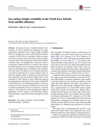
Fig. 1 a Observed SSV (m) in the North East Atlantic. The black
contours show the 300 and 500 m bathymetry isolines. b Monthly
SLA for the DaNS area. c Annual cycle of SSV for the DaNS area in
the North Sea and a location near the continental shelf edge, off the
west coast of Ireland (see legend and Panel a). d Correlation between
box-average SLA (DaNS area) and the local SLA elsewhere
4. P. Sterlini et al.
1 3
the DaNS area. We also test with atmospheric pressure
at sea level (SLP) as an indication of a pressure gradient
which acts remotely.
Additional components that can (of course) be added
to this list of potential SSV drivers. Generally this will
be dependent upon the specific region and for areas other
than the North Sea we would probably need to consider
drivers that are more specifically related to those regions.
For example, in our analysis of the SSV in the Indonesian
archipelago region (not presented), the NINO 3.4 index and
the Pacific Decadal Oscillation index were found to be sig-
nificant in describing the SSV.
A first order estimate of the potential relevance of a can-
didate SSV driver is provided by its correlation with SLA
in the desired target area, though it is noted that a high cor-
relation does not necessarily imply a physical or dynamical
relation between the driver and the SLA.
2.3 Linear regression model (LRM)
A multiple LRM is constructed using (a subset of) the driv-
ers above to test how well they can describe local SSV. The
most general LRM formula is:
where αi(x, y) indicates the regression coefficients
(determined locally), Fi(x, y, t) the driving mecha-
nisms (not necessarily local), and ǫloc(x, y, t) a local
residual error. The inclusion of auto-regressive terms
(sshloc(x, y, t − j), j = 1, 2, . . .) in the right hand side of the
above equation is not considered at this stage, although it is
known that memory is generally important for SSV (Dan-
gendorf et al. 2014b).
The inclusion or exclusion of the forcing mechanisms
identified above will lead to a reconstructed SLA with vari-
ous degrees of fit to the observed sea levels. It is assumed
that higher correlation between reconstructed and observed
sea level indicates a better representation of the variability
described by the selected combination of forcing mecha-
nisms. Following Calafat et al. (2013) we also test for
explained variance which takes both variability and the dif-
ferences in the amplitude between the observed and mod-
elled sea surface into account. Explained variance is com-
puted as:
where y denotes SLA and yi denotes the reconstructed
SLA, or simply a particular component. Because of the
relatively short time-span of the altimeter data (21 years)
we use the entire period for both constructing and testing
(1)
sshloc(x, y, t) =
i
αi(x, y)Fi(x, y, t) + ǫloc(x, y, t)
(2)EVi =
var(y − yi)
var(y)
our linear statistical model. In addition we have tested the
robustness of these results by using only the first third of
the data to train the model and testing it on the full data set.
2.4 Cross‑correlations and multi‑collinearity
A fundamental problem encountered in any multiple linear
regression approach is that the candidate driver compo-
nents (i.e. the possible regressors) may not be statistically
independent from each other. This inter-relation between
components not only obscures the interpretation of the
results (especially the partitioning) but also inflates their
confidence estimates. In statistical literature this problem is
known as multi-collinearity.
Here we use a simple and objective method to assess the
relevance of a particular regressor in a statistical model.
This method is based on the variance inflation factor (VIF).
The VIF of a particular regressor in a regression model
measures to what extent this regressor can be understood
from a linear combination of the other regressors. For a
given regression model with Fj, j = 1, 2, . . . n regressors,
the VIF of component Fi is given by:
where R2
i is the squared correlation between Xi and Xfit,i
with Xi = Xfit,i + ǫ and Xfit,i = c0 + j�=i βjXj. A compo-
nent is completely independent from the other components
if its VIF is unity. There is however no upper-bound to the
VIF.
Based on VIF analysis a straightforward stepwise
regressor selection method is employed. Starting with all
regressors, in the first round of selection we compute all
VIF factors and remove the regressor with the highest VIF
if it is larger than a predefined threshold of 2. From Eq. 3
this corresponds to a correlation of 0.5, meaning that if at
least 25 % of a regressor’s variance can be explained by the
remaining regressors, it will be discarded. After this regres-
sor has been removed from the model the VIF factors are
determined again, isolating a second possibly “redundant”
regressor. This procedure continues until all remaining
VIF factors are below the desired threshold. This stepwise
approach means that ultimately we end up with a number
of drivers that can describe other parameters but which can-
not themselves be described and are statistically distinct
from each other (R is less than 0.5). This facilitates subse-
quent interpretation.
It is important to note that the independence of data does
not mean that it is a relevant descriptor or forcing mecha-
nism for a change in sea level. Connection of a data set with
an underlying physical process is therefore of paramount
importance and ultimately data to be included or excluded
in the LRM is subject to such a physical motivation.
(3)VIFi =
1
1 − R2
i
5. Sea surface height variability in the North East Atlantic from satellite altimetry
1 3
Ideally, the hierarchical selection is carried out locally
because different local areas may experience very different
driving mechanisms. This is true for the North Sea where
Chen et al. (2014) and Dangendorf et al. (2014a) showed
that the it can be divided into different regimes which are
dominated by either wind or SLP. This consideration also
holds for the area over which spatial averaging is carried
out (SSV of the GMSL encounters different drivers than
local sea level of the Bay of Bengal, for example). How-
ever, when representing results graphically on a map it may
destroy their spatial coherence if different components are
used in nearby locations. We therefore apply the VIF-based
method to our target area (discussed below) and subse-
quently use those components for the entire domain.
3 Data and pre‑processing
Daily gridded mean sea level anomaly (SLA) data for the
NEA area were downloaded from AVISO for the period
1993–2013 at 0.25° spatial resolution. The “all-sat-merged”
product is used, to which standard corrections, including
the Dynamic Atmospheric Correction, have been applied as
documented in the AVISO Handbook (AVISO 2014). Daily
zonal and meridional wind speed at 10 m height (u10 and v10
respectively), atmospheric pressure at sea level (SLP) and
sea surface temperature (SST) were downloaded from the
Global Reanalysis ERA-Interim dataset (Dee et al. 2011). In
using SST we assume that the surface layer in shallow waters
is well mixed. This assumption is validated through a com-
parison between the SST field and vertical mean temperature
(VMT) data based on 3D ocean temperature from the ORAS4
ocean reanalysis model (ECMWF 2015). VMT is not directly
used here as the product assimilates altimetric SLA (ECMWF
2015) so is excluded for reasons of consistency. ICOADS 2°
enhanced surface wind stress was downloaded from NOAA/
OAR/ESRL PSD (2015) (meridional, UST; zonal, VST).
Monthly values of the North Atlantic oscillation index (NAO)
were downloaded from CRU/UEA (2014) through the KNMI
Climate Explorer website (www.climexp.knmi.nl).
To remove the trend associated with the changing
mass of the oceans we subtract the GMSL from the SLA
field. Since this also removes the global mean, only pro-
cesses which act regionally in the time series remain. Only
monthly mean fields are used to remove temporal high-fre-
quency variability in all fields. In addition we subtract the
multi-year monthly means over the period 1993–2013 for
all fields to remove the basic seasonal cycle.
Low frequency signals can alias as a long term trend in
a relatively short altimetry record of 21 years. Since regres-
sion models are unable to separate these decadal fluctua-
tions from long term trends, stationarity of the underlying
time series is required. To address this we linearly detrend
all time series. However, Frankcombe et al. (2014) demon-
strated that removing linear trends based on short term data
may lead to biases. We therefore test for the robustness of
the regression coefficients used in the LRM. Thus our study
is based on the SSV of detrended monthly anomaly fields.
4 Observed regional SSV
Figure 1a shows the mean SSV pattern by means of the
standard deviation of the monthly SLA over 21 years for
the NEA. The SSV pattern is rich in structure and charac-
terised by large regional differences. Strong SSV is seen
in the North Sea with a maximum of around 14 cm off the
west coast of Denmark (DaNS area). There are isolated ‘hot
spots’ of high SSV in the English Channel, as well as a dif-
fuse region of high SSV in the Atlantic Ocean that coincides
with the tail end of the Gulf Stream. Approximate bathym-
etry is also shown and seems to indicate areas of low varia-
bility near the edges of the continental shelves. The monthly
time-series of SLA in the DaNS region is shown in Fig. 1b.
In the construction of the monthly SLA values we
removed the mean seasonal cycle. However the SSV of the
SLA contains a seasonal cycle; the mean standard deviation
of all SLA values over the 21 year period for each month
are shown in Fig. 1c for two subregions: the DaNS area and
a region at the continental shelf edge off the west coast of
Ireland. Both regions are indicated in Fig. 1a. For the DaNS
area the variability peaks in the winter months; we will see
in the next section that this is consistent with a variability
forcing dominated by wind. Near the continental shelf edge
the SSV remains rather low throughout the year.
Figure 1a, c show that SLA displays regional behaviour
with marked differences. However, this does not imply that
there is no spatial coherence within the SLA field. On the
contrary, certain areas display a surprisingly high degree of
spatial coherence, especially those over shallow continental
shelf seas such as the North Sea. As the DaNS area in the
North Sea is our area of interest (Fig. 1) it is instructive to
reveal this coherence with respect to that particular region.
Figure 1d shows the correlation between SLA in the
DaNS area and local SLA elsewhere. As expected this cor-
relation is near unity in the vicinity of the DaNS box but it
remains surprisingly high in much of the entire North Sea
basin before rapidly becoming insignificant off the conti-
nental shelf. This is an indication of strong spatial coherence
over the entire North Sea shelf. This spatial coherence is a
common feature of (shallow) shelf seas worldwide (Hughes
and Meredith 2006). However, we note here that the coher-
ence that is clearly visible on the shelf does not extend into
the English Channel which suggests that this region experi-
ences different processes in driving SSV than in the DaNS
region. This may be due to differences in water depth,
6. P. Sterlini et al.
1 3
coastal geometry and local meteorology, and highlights the
spatial variation in the predominant causes of SSV.
5 Understanding regional SSV
A picture emerges from the previous section of a locally
substantially different SSV that might be explained from a
combination of different driving mechanisms. In Sect. 2 we
explained the methodology that will be used to determine
what those driving mechanisms might be. Here we present
and explain the results from this analysis with attention to
the processes acting behind the drivers, where applicable.
5.1 Local field parameters
Local correlation maps for SLA with u10, v10, SLP and
SST are shown in Fig. 2. The figure shows that there is a
clear spatial structure in the correlation patterns in the
North Sea for the wind components (and SLP which partly
drives the wind). The wind components u10 and v10 are
coupled and on monthly time-scales largely follow the
atmospheric pressure distribution. However, which of the
two components play the most significant role in driv-
ing SLA in a given location is strongly dependent on the
coastal geometry.
Correlations of SLA with zonal wind speed (u10, east-
ward wind defined positive) are very high and positive
(maximum values above 0.9) in most of the North Sea
basin (and extending along the Norwegian coast line). The
correlation between u10 and SLA decreases as we go fur-
ther north and off the continental shelf. This near-coastal
zone influence of the wind on SLA is found throughout
the world but is extremely clear in the North Sea. Negative
correlations are found off the north coast of Scotland and
along the west of Ireland.
The structure of the correlation map with meridional
wind speed (v10, northward wind defined positive) is very
Fig. 2 Correlation maps between local SLA and field parameters;
u10 (upper left), v10 (upper right), SLP (lower left) and SST (lower
right). Statistical significance of the correlations has been assessed on
the basis of the Fisher z-transform. Crossed where non-significant at
95 % confidence level
7. Sea surface height variability in the North East Atlantic from satellite altimetry
1 3
different from that of u10. Positive correlations between
SLA and v10 are found off the west coast of the UK and off
the Norwegian coast, and a region of negative correlation
is evident against the east coast of the UK. Respective cor-
relation maps with UST and VST (not shown) show simi-
lar spatial patterns as with wind speed, but exhibit a more
gridded structure due to the lower resolution of the surface
wind stress data than the SLA.
The overall picture of the SLA response to wind forcing
is one of Ekman transport, and is in line with results found
by Dangendorf et al. (2014a) who used tide gauge records
to assess the barotropic response of the North Sea to atmos-
pheric forcing; longshore components of wind dominate
the SLA everywhere along the coast in the North Sea basin.
Specifically, Ekman transport in the open ocean is gener-
ated by the northward winds which results in a net move-
ment of water towards the east and against the UK coast.
Similarly, Ekman transport within the North Sea basin is
generated from eastward winds leading to a southward
movement of water against the Dutch and German coast-
lines. In these cases the coastlines induce a convergence of
water and a subsequent SLA response through mass con-
servation. This response of the SLA to wind appears to be
largely confined to the shallow seas on the continental shelf
and therefore suggests that wind is the primary forcing
mechanism of SSV in the North Sea.
The correlation pattern of SLA with SLP shows high
positive values off the east coast of the UK and to the
north of Scotland and weakly negative values to the west
of France and off the Danish coast. This pattern is broadly
similar to the inferred correlation patterns seen in model
simulations performed by Chen et al. (2014) who tested
for the IB effect induced by local SLP. However, we note
that the correlation seen in Fig. 2 exists even though the
inverse barometer correction has been applied to the altim-
eter data. This implies that whilst the SLP does not repre-
sent an actual physical connection with SLA, the correla-
tions seen here may be due to the SLP acting though other
(non local) forcing factors such as wind. This is explored in
more detail in Sect. 6.3.
The final local driver we consider is SST which is used
here as a measure of the heat content of the local well
mixed waters. We therefore expect to find increasing sea
levels with increasing values of SST due to thermal expan-
sion of the water column. The spatial pattern of the cor-
relation between SLA and SST seen in Fig. 2 is generally
positive with high values folding around southern Iceland
towards Scotland. This positive correlation with SST con-
firms our expectation that sea level is generally higher with
warmer SSTs.
5.2 The DaNS area (1): local drivers and remote
forcing
We now provide further detail for the DaNS area. Table 1
lists the correlation coefficients between monthly SLA
over the DaNS area and the tested field drivers. Wind speed
(WS) and zonal and meridional wind stress (UST and VST
respectively) are included for completeness. Of the tested
local SSV drivers, zonal wind clearly stands out as being
most important, consistent with Fig. 2.
Correlation between SLA and SLP in the DaNS is not
significant (also see Fig. 3f). As the local SLA response to
local SLP is the IB effect (Dangendorf et al. 2014a) this
hints that the DAC correction (including IB) applied to the
altimetry data is correct in the DaNS region as it removes
the wind and pressure effects for periods below 20 days and
the IB effect for periods larger than 30 days (AVISO 2014).
Up to now we have tested only the correlation between
the SLA and a driver (for example, the wind) at the same
location. However, especially in near coastal zones where
bathymetry, coastline geometry and other effects may be
important, it can be argued that one should relax this con-
dition of examining colocated SLA and driver fields. In
this section we therefore expand the colocated correlation
analysis to a local SLA (box average over the DaNS area)
to a driver over a field with the aim of ascertaining whether
there is a spatial pattern in forcing SSV by drivers from a
remote location.
Figure 3 shows the correlation between the box average
SLA over the DaNS area and fields of wind parameters,
SLP and SST. It is clear that the influence of u10 on SLA in
the DaNS area is a large-scale pattern. In fact, the highest
correlations are found in an area to the North of the DaNS.
Negative correlations up to −0.6 also exist between u10
and SLA in the DaNS off the South of Spain. This nega-
tive correlation comes about because the wind field itself is
forced by large-scale pressure differences. Indeed, a simi-
lar but displaced correlation structure is seen in the panel
showing correlation with SLP (lower left). Note that the
SLP correlation structure supports the predominance of
eastward wind and its effect on SLA in the DaNS region,
though in itself does not have a direct role in driving local
SLA (Wakelin et al. 2003; Dangendorf et al. 2013).
Table 1 Correlation between
SLA and possible field
parameters for the DaNS area
NS not significant at the 95 % confidence level
Field driver u10 v10 UST VST WS SST SLP
SLA (DaNS) 0.84 −0.13 0.84 NS 0.37 0.36 NS
8. P. Sterlini et al.
1 3
The correlation map with the v10 field nowhere yields
correlations above 0.4, and shows less spatial structure than
the maps from u10 and SLP. The highest correlations are
seen in the Atlantic Ocean off the west coast of Ireland and
indicates that strong northward winds in the Atlantic lead
to increasing levels of SLA in the DaNS. Meridional wind
may be important because it’s inherently coupled with the
more dominant zonal wind component in the DaNS region.
Indeed, prevailing winds drive cyclonic circulation within
the North Sea basin which can lead to increased sea lev-
els towards the DaNS area Dangendorf et al. (2014c). An
alternative view is that an anticyclonic wind system with
low pressure over the UK or a cyclonic system centred
over Norway leads to wind set up in the DaNS. However,
in light of the SLP correlation map and the DAC correc-
tion applied to the altimeter data which removes high fre-
quency (20 days) atmospheric responses, this explanation
is tenuous. It is more likely that the meridional winds are
correlated with SLA in the DaNS due to Ekman transport
into the North Sea, implying that there is a remote forcing
off the west UK coast.
Correlations with SST are quite low and attain a maxi-
mum near the DaNS area itself. Interestingly the pattern
is rather consistent along the coast which could be in part
related to upwelling/downwelling.
It is interesting that the correlation results presented here
are in line with those found by Dangendorf et al. (2013)
who performed a similar analysis using observations of
sea level taken from the Cuxhaven tide gauge (situated to
the south west of the DaNS region). In that study correla-
tions were performed using data from 1871 to 2008. The
consistency between the long term study at a fixed loca-
tion and the work presented here with a spatial analysis
over a shorter time span is a strong indicator of the stability
in time between the local wind and local sea level in this
region.
Fig. 3 Correlation maps between box average SLA over the DaNS
area and u10 (upper left), v10 (upper right), SST (lower left) and
SLP (lower right). Statistical significance of the correlations has been
assessed on the basis of the Fisher z-transform. Crossed where non-
significant at 95 % confidence level
9. Sea surface height variability in the North East Atlantic from satellite altimetry
1 3
5.3 Remote drivers
We now look at remote drivers of SSV. The correlation pat-
tern for the NAO is shown in Fig. 4. Whereas several stud-
ies have shown that highest correlations between the NAO
index and the sea level in the North Sea occur at decadal
time scales and in the winter months (e.g. Yan et al. 2004;
Tsimplis and Shaw 2008; Chen et al. 2014) correlations
using monthly data through all seasons also show a clear
spatial structure. Highest positive correlations (around 0.6)
with SLA are seen in the eastern parts of the North Sea,
extending northwards off the coast of Norway. Negative
values of up to −0.4 are found to the east of Iceland and
in the Mediterranean. The NAO correlation map is broadly
similar to those of SLP and u10 (Fig. 2), consistent with the
findings from Dangendorf et al. (2013). This is not surpris-
ing as the NAO is defined as a pressure difference and the
large-scale wind on monthly time-scales is geostrophically
balanced.
5.4 The DaNS area (2): identification of forcing
mechanisms
The similarity of the correlation patterns found between
parameters in the previous section make it very clear that
significant cross-correlations occur between the drivers.
Here we focus on the DaNS area to examine this more
fully. Table 2 shows the full cross-correlation matrix of
SLA and the tested drivers for the DaNS area. Apart from
the local drivers that have already been discussed, high cor-
relations are found with NAO (0.48). However, the corre-
lation between NAO and u10 is also high (0.54) which is
consistent with an index based on atmospheric pressure dif-
ferences and resulting wind patterns.
In the previous sections we presented a number of poten-
tial drivers of SSV in the NEA. The correlation coefficients
between those and the SLA help to paint a picture which
identifies the primary forcing mechanisms. u10 and SST
show significant correlation with SLA and low cross corre-
lations with other potential drivers. v10 is included for con-
sistency with the wind being a vector rather than a scalar
quantity. Table 1 shows that SLP has an insignificant local
correlation with SLA in the DaNS area as expected. At this
stage it is excluded from the LRM model. Climate indices
are inherently representative of a number of higher level
forcing mechanisms which act behind them and which in the
ideal case we are seeking to identify. For example, the NAO
affects wind, pressure and SST which means that a change
in the NAO subsequently brings about corresponding baro-
clinic and barotropic responses from the ocean (Chen et al.
2014). We saw from Table 2 that there is a strong cross cor-
relation between the NAO and u10 which suggests that much
of the NAO signal can be captured using wind. Note that we
will test this assumption with the VIF analysis in Sect. 6.4.
The NAO is therefore also excluded from the LRM at this
stage. u10, v10 and SST are thus identified from the simple
physically motivated correlation analysis.
Fig. 4 Correlation maps between local SLA and NAO. Statistical
significance of the correlations has been assessed on the basis of the
Fisher z-transform. Crossed where non-significant at 95 % confidence
level
Table 2 (Cross-) correlation
between tested local and remote
forcing mechanisms for the
DaNS area in the North Sea
(5°–7°E 54°–56° N) and SLA
DaNS SLA u10 v10 UST VST WS SST SLP NAO
SLA X 0.84 -0.13 0.84 NS 0.37 0.36 NS 0.48
u10 X NS 0.95 NS 0.55 0.21 -0.2 0.54
v10 X NS 0.88 NS NS -0.26 0.4
UST X NS 0.53 0.26 -0.21 0.52
VST X 0.26 0.13 -0.33 0.43
WS X NS -0.45 0.35
SST X NS 0.17
SLP X NS
NAO X
Figures in blue and red indicate values above an arbitrary value of 0.35; blue for correlation against
SLA, red for cross-correlation with another driver
NS denotes not significant at the 95% confidence level
10. P. Sterlini et al.
1 3
In Sect. 2 we described an alternative method to iden-
tify relevant drivers by using VIFs. In this method VIFs are
used to detect possible regressors that are well explained by
linear combinations of other regressors. If the VIF-method
is applied to DaNS area, SLP is added to the above list of
relevant regressors, but excludes the NAO based on statisti-
cal significance. For this we have used a VIF threshold of
2. This means that a multiple LRM with SLP in addition to
the other identified components, yields a strong increase in
explained variance. In the next section we present results
for both subsets of drivers, with and without SLP. We also
explore the role of SLP as a descriptive parameter of SSV
and seek to identify an underlying physical explanation for
its apparent involvement in affecting SSV in the North Sea.
6 Statistical modelling of regional SSV
In this section we test the effect of the forcing mechanisms
identified in Sect. 5.4 on driving SSV. A multiple LRM is
used to test this hypothesis where we make the assump-
tion that a good correlation between observed SLA and
modelled SLA signifies a good capture of the SSV driv-
ers. We also use explained variance which takes account of
the amplitude of the variation between a parameter and the
observed SLA.
We start with the inclusion of local wind (u10 and v10)
and local SST in the LRM as these are the drivers identified
by the simple correlation analysis with the highest corre-
lation coefficients. We then test with SLP as an additional
driver as identified from the VIF-optimised regressor selec-
tion method. As already explained in Sect. 2 the VIF-opti-
misation was carried out for the DaNS area and the same
regressors are then used for the entire NEA domain for
consistency.
6.1 Reconstruction and explained variance
The top panels in Fig. 5 show the correlation between the
observed and the reconstructed SLA using the two sets
of forcing parameters as regressors. Explained variance
is given below. The general pattern seen in each panel is
similar; highest correlations and explained variance are
seen in the North Sea, extending from Denmark towards
the entrance to the North Sea in the north west. Correla-
tions greater than 0.5 appear to be confined to the rela-
tively shallow waters (less than 300 m) on the continental
shelf. The suggestion that water depth plays a role in SSV
is seen clearly near the Norwegian Trench where local
water depths exceed 300 m and correlations are (strongly)
reduced. Adding SLP as an additional regressor in the
LRM, as motivated by the hierarchical VIF-selection, sub-
stantially increases the footprint size of high correlation
and explained variance values in the North Sea, towards the
east coast of the UK (right panel). The correlation between
observed and modelled SLA in the DaNS area increases
from 0.87 to 0.91.
Figure 6 provides further detail for the VIF-based model.
Since the VIF-based model explains more than 80 % of
the variance it comes as no surprise that the residual (left
panel, vertical dashes) is much smaller than the observed
SLA (red circles). The model captures the slow variations
(5-year running averages) quite well. In fact, the VIF-based
model provides a rather good estimate of the entire SLA
distribution between the 5-th 95-quantile, as can be inferred
from the quantile-quantile plot (right panel, red triangles)
and only weakly underestimates the very low and high
extremes.
It may seem obvious that the highest correlations are
found for the DaNS area given that the parameters used
in the LRM are selected based on our detailed analysis of
the DaNS area; the LRM is effectively optimised for this
region. Indeed the high SSV region in the open North
Atlantic Ocean as identified in Fig. 1 (top-left) is not very
well reconstructed with the parameters chosen here, imply-
ing that none of them can be classed as significant drivers
of SSV in this region. The hot spots of high SSV in the
English Channel have also not been reproduced as differ-
ent forcing factors for SSV come in to play in a differing
region, despite its relative proximity to the DaNS. In this
case, the dominant process behind SSV in the DaNS region
(u10) is not responsible for the SSV that seen in the Eng-
lish Channel.
6.2 Regression patterns
We now take a closer look at the regression coefficients that
appear in the LRM (using drivers identified from the VIF
regression for the DaNS area). High regression coefficients
indicate a high sensitivity of SLA to the predictor. We scale
these regression coefficients by their standard deviation
so that they can be compared against each other. Figure 7
shows the regression coefficients and explained variance
patterns (REVP).
The REVP of u10 shows a clear similarity to the spatial
pattern visible in Fig. 5; a region of high explained vari-
ance exists off the west coast of Denmark. This indicates
the high dominance that u10 has over the other regressors
in explaining SSV in this region. The pattern for meridi-
onal wind is very different. High values are found north-
ward from Spain and along the west of the UK (confined to
the continental shelf) and the west of Norway. These results
appear to be consistent with the findings of Calafat et al.
(2012), Calafat and Chambers (2013) and Dangendorf et al.
(2014a) who identify remote boundary wave forcing as a
driver for SSV in this region brought about by changes in
11. Sea surface height variability in the North East Atlantic from satellite altimetry
1 3
v10 along the continental slope. Dangendorf et al. (2014a)
further note that this forcing is not purely local because the
propagation of the coastally trapped waves will affect SLA
at all points along its path.
The REVP for SLP is positive throughout the North Sea
and not relevant offshore from the continental shelf. SLP
explains the variance of the SLA most strongly in a region
off the east coast of the UK. Patterns for local SST is spa-
tially rather uniform over the North Sea area with positive
coefficients everywhere, implying higher SLA if the local
SST is warmer, due to the thermal expansion of the mixed
surface layer. Values for explained variance of are highest
along the continental shelf, and to the north of Scotland.
6.3 The remote effect of sea level pressure (SLP)
on SSV
As we noted earlier, Fig. 2 shows a significant correlation
between SLP and SLA. Further, the VIF analysis identi-
fies SLP as a descriptive parameter for SSV (Fig. 7) which
appears to be at odds with Fig. 3 which shows that SLP has
no local role on the observed sea level in the DaNS region.
Assuming that the IB correction holds in the North Sea, the
implication is that SLP may exert an effect on SLA through
a remote mechanism. We therefore test here the remote
forcing effect that SLP exerts on the SLA within the North
Sea basin.
Fig. 5 Top Correlation maps between observed and reconstructed sea
surface height over the period 1993–2013. Only correlations larger
than 0.5 are coloured. Left (Local) u10, v10, and SST are included.
Right SLP is also included. Explained variance is given beneath. Con-
tours show the 300 and 500 m bathymetry isolines. Statistical signifi-
cance of the correlations has been assessed on the basis of the Fisher
z-transform. Crossed where non-significant at 95 % confidence level
12. P. Sterlini et al.
1 3
Figure 8 shows correlation maps between SLP and the
box average SLA for 3 additional locations in, and to the
north of the North Sea basin (upper right, lower left and
lower right respectively). In contrast to the DaNS region
(upper left panel) we note significant correlation between
SLP and SLA within these 3 regions. This points towards
a physical process which is driven by SLP and exerts an
effect which varies spatially.
In a meteorological setting, external surges can be gen-
erated by pressure systems passing the northern entrance
region of the North Sea. However, this is not likely to be
what we see here as this effect will have been removed from
the SLA data through the DAC correction. Instead it is more
likely that there is a remote influence of wind expressed in
the SLP gradient. The spatial structure within the correla-
tion maps for the boxes within the North Sea basin suggests
an eastward wind pattern at the North Sea entrance. This
would lead to Ekman transport directed into the North Sea,
propagating along the UK coastline and increasing the sea
level along the UK east coast. For the region outside of the
basin (lower right panel) we see an inverted correlation pat-
tern where this effect no longer holds.
The overall picture is that local eastward wind explains
the variance of the SLA in the DaNS region, and to a lower
degree, that remote eastward wind explains the variance
towards the west of the North Sea basin. This regional
dominance of a given parameter over another in the North
Sea has previously been noted by Chen et al. (2014) and
Dangendorf et al. (2014a). These results show that the VIF
analysis is a useful tool in isolating descriptive parameters
of SSV which can be used in LRMs if underlying physical
processes can be identified.
6.4 VIF‑optimised versus ‘full’ model: Does it make a
difference?
One question that comes to mind is whether, and if so how,
can the LRM be extended? For example, does the cor-
relation pattern between observed and reconstructed SLA
change much if we include all regressors regardless of their
possibly high VIF values and regardless of their cross-cor-
relations. Figure 9 shows a representation of the monthly
SLA time series for the DaNS area using (left) the VIF-
optimised regressor selection, and (right) the ‘full’ model
with all regressors stated in Sect. 2. Each row indicates the
contribution from a particular regressor and oblique dashes
are used to indicate VIF-excluded components and com-
ponents that are found to be non-significant following a
standard t-test. As one can see the full VIF model includes
UST as well as u10. These parameters are known to covary
and including both in a LRM model would not make sense.
This provides confidence in the VIF optimisation process.
(In fact the optimised VIF model selects VST in preference
over v10; v10 is used in the LRM as it is coupled with u10
which is more dominant than UST.) Otherwise the differ-
ences between the approaches are marginal for the DaNS
area. Those components that are excluded in the VIF-meth-
odology are found to be non-significant in the ‘full’ model
(right panel) which notably holds for the NAO.
1995 2000 2005 2010
−20
−10
0
10
20
Date
SLA[cm]
obs
resid
obs−5yr
mod−5yr
resid−5yr
COR(obs,mod)= 0.91
P05
P25
P75
P95
P05 P25 P75 P95
Observed SLA [cm]
ReconstructedSLA[cm]
−20 −10 0 10 20
−20
−10
0
10
20
scatter
qqplot
Fig. 6 Left Time series of the observed DaNS SLA (red circles) with
vertical dashes indicating the residuals from the VIF-based model.
Running-average values over 5 year periods as indicated by the leg-
end are also shown. Right Scatter of observed and reconstructed
DaNS SLA (black) and quantile–quantile plot (red), with lines indi-
cating empirical quantiles (blue)
Fig. 7 Regression coefficients and explained variance for the VIF-
optimised LRM model for u10, v10, SLP and SST in the multiple
regression model. Statistical significance of the correlations has been
assessed on the basis of the Fisher z-transform. Crossed where non-
significant at 95 % confidence level
▸
13. Sea surface height variability in the North East Atlantic from satellite altimetry
1 3
14. P. Sterlini et al.
1 3
Fig. 8 Correlation maps between box average SLA and SLP for a
number of locations in the North Sea (solid box). Figure 3 is repeated
here for ease of comparison in upper left. Dotted boxes show location
of DaNS. Statistical significance of the correlations has been assessed
on the basis of the Fisher z-transform. Crossed where non-significant
at 95 % confidence level
1995 2000 2005 2010
DaNS cor= 0.91 (VIF−optimised)
Year
sla
fitted
resid
u10
v10
ust
vst
sst
slp
nao // = VIF−excluded
= N.S. at 95%
1995 2000 2005 2010
DaNS cor= 0.92 (COMPLETE MODEL)
Year
sla
fitted
resid
u10
v10
ust
vst
sst
slp
nao = N.S. at 95%
−20
−10
0
10
20
cm
Fig. 9 Representation of the monthly SLA time series from VIF analysis for the DaNS area. VIF-optimised model (left) and full model (right).
N.S. not significant
15. Sea surface height variability in the North East Atlantic from satellite altimetry
1 3
The findings here therefore suggest that there are no
additional parameters from our initial start point which can
be used to improve the LRM. That’s not to say that there
are no further covarying parameters which can be used to
describe the SSV in the DaNS region, and indeed we note
that whilst the inclusion of more parameters may appear
to increase the general performance of the LRM, it is done
so at the risk of instability when using the model in a pre-
dictive capacity. We therefore assert that the LRM is valid
only for the 21 year period in which the SLA and regressor
data is present.
However, in order to test the robustness of the LRM we
train it using the first third of the data and test it on the full
data set. We find that there is no degradation of the result
with correlation coefficients and explained variances are
not significantly altered.
6.5 Memory in the ocean: introducing autoregressive
terms in the LRM
Sea level anomalies are long-lived in the open ocean once
they are excited (Hughes and Williams 2010). This means
that a natural way in which the LRM can be extended is
by including lagged SLA terms (“lag-1” and “lag-2”) as
additional regressors. In these cases the SLA information
of the previous or 2 months is used to predict the SLA
at month 0. This provides information on how much of
the signal can be understood from simple persistence in
time. The inclusion of these auto-regressive terms has a
huge impact on the correlation maps off the continental
shelf. Figure 10 (upper panel) shows this correlation map
where the VIF optimised model is used, but in addition
the lag-1 and lag-2 month autocorrelations are included.
The inclusion of these two terms does not change any-
thing on the continental shelf but dramatically improves
its accuracy in the open ocean. The regression coefficients
(shown in the lower two panels) confirm that they play an
important role in the regression. Whereas the lag-1 regres-
sion field is predominantly positive over the open ocean,
the lag-2 field is much smaller and mostly negative, thus
revealing a typical time-scale of 1–3 months for the eddy-
ing phenomena.
7 Conclusions
To increase our understanding of sea surface height varia-
bility (SSV) in the North East Atlantic we analyse monthly
altimeter data. Particular focus has been on a region of high
SSV off the Danish coast, referred to as the DaNS area.
Variability in that region is high, as it is in a large part of
the North Sea. Since the GMSL has been removed from
the data and we also use linear detrending, our attention is
turned towards variability in sub decadal time scales and
not trending analyses.
The approach undertaken in this work to test and apply
potential SSV forcing mechanisms in both the local and
remote context has provided a spatial awareness of the
processes which act across the region. We have identified
a number of key drivers and have constructed a statistical
model that is able to explain more than 80 % of the vari-
ance in that region using information relating to local wind
and SST conditions as well as atmospheric pressure which
exerts a remote influence on the SLA through it’s gradi-
ent and subsequent wind forcing. It appears unnecessary
at these monthly time-scales to include information from
large-scale drivers like the NAO which has been shown
to be important in decadal scale SSV in the North Sea
(e.g. Tsimplis and Shaw 2008; Chen et al. 2014), though
it is noted that using seasonal or derivative indices such as
NAO+, NAO−, RDG and GS as defined by Cassou et al.
(2004) may increase the explained variance, especially dur-
ing the winter months. Off the continental shelf, the statisti-
cal model performs rather poorly (correlations below 0.5),
yet a powerful way to increase its performance is to include
an auto-regressive term.
The LRM provides spatial information on the response
of the North Sea to a number of parameters with underly-
ing physical processes which describe the observed SSV
in the DaNS area well, and confirms findings from previ-
ous studies. The importance of long shore winds in the
North Sea basin found by tide gauge studies (Calafat et al.
2013; Dangendorf et al. 2013) is seen here with the areal
data afforded by altimetry. The use of altimetry data here
has also shown not only the linkage between a parameter
and local SSV at a specific location, but also spatial pat-
terns from which further inferences can be made relating to
SSV over the model domain, for example, the role of SLP
in forcing a non isosteric ocean response through Ekman
pumping.
In addition to providing a spatial awareness of the local
and remote factors affecting the SSV in the North Sea over
the 21 years of observational data, the regression coeffi-
cients in the LRM show a stability over time; those derived
from the first 6 years of data and applied to the complete
21 year data period lead to a modelled sea level which is
not significantly different to the results presented here. This
provides confidence in extending the model with either
historical or forecast data. VIF analysis has been used to
introduce a degree of objectivity in identifying parameters
which can be used in the LRM, though these are subject
to an insight and understanding of the underlying physical
processes at work in them.
Although ’tuned’ for the DaNS regions, the methodol-
ogy used here is a general approach which can be extended
and applied to other regions. The inclusion (or exclusion) of
16. P. Sterlini et al.
1 3
additional parameters into the LRM will be location specific,
and likewise provide an insight into the SSV in a spatial con-
text. In particular, the spatial advantage that satellite altim-
etry holds will assist in addressing the issue of how oceanic
signals are transmitted through the shelf to the coast.
There are clear limitations in this work. An inherent weak-
ness in that whilst the LRM model appears to be stable in
time and shows potential for extension for longer periods, the
model is based on data which is limited in duration to that
of the satellite altimetry era. This means that only high fre-
quency (i.e. sub decadal) forcing mechanisms can be identi-
fied. Further, the model is optimised for the DaNS region, with
parameters identified as being most relevant here and applied
throughout the model domain. The dominance of forcing
0.5
0.6
0.7
0.8
0.9
1.0
−20 −15 −10 −5 0 5 10
45
50
55
60
65 VIF_WITH_LAGS
Correlation between observed and reconstructed SLR
−5
45
50
55
60
65
45
50
55
60
65LAG1
Regression coefficient for LAG1
−5
0
5
cm/sd
−20 −15 −10 −5 0 5 10 −20 −15 −10 −5 0 5 10
LAG2
Regression coefficient for LAG2
Fig. 10 Correlation between observed and reconstructed sea surface
height over the period 1993–2013. Only correlations larger than 0.5
are coloured. Upper ‘VIF optimised’ model + lag-1 and lag-2 month
SLA. Contours show the 300 and 500 m bathymetry isolines. Statisti-
cal significance of the correlations has been assessed on the basis of
the Fisher z-transform. Crossed where non-significant at 95 % confi-
dence level. Bottom row patterns of the regression coefficients of the
(left) lag-1 and (right) lag-2 SLA component used in the construction
of the upper panel
17. Sea surface height variability in the North East Atlantic from satellite altimetry
1 3
parameters has been shown to vary over the region (for exam-
ple, u10 is dominant in the east of the North Sea basin; SLP in
the west) and this is manifest in magnitude of the local regres-
sion coefficients. For simplicity here, no account has been
taken into regarding an entirely different selection of param-
eters to be used across the model and applied locally and we
have focussed here on the DaNS region which exhibits the
highest levels of SSV in the model domain.
Whilst local wind was shown to be a dominant driver of
SSV in this region, no account is made that the response
of the ocean to wind forcing is not purely local because
information can be carried along the coast by boundary
waves (Sturges and Douglas 2011; Calafat and Chambers
2013; Dangendorf et al. 2014a). Additionally we have not
considered any explicit terms to account for mass-loss
changes from glaciers and ice-sheets. As the time-series
we have considered here are relatively short, the mass loss
contributions which are approximately linear have been put
‘silently’ removed by linearly detrending the data. Neither
have we explicitly included specific oceanic processes,
such as ocean circulation, movement of transient features
or Rossby wave propagation (Calafat and Chambers 2013).
We have carried out tests that augment the LRM with
a 0–700 m heat content regressor, as could for example
be obtained from the ECMWF ocean reanalysis ORAS4
model. However that ocean reanalysis product assimi-
lates altimetric SLA (ECMWF 2015) so it was excluded
for reasons of consistency. SST was found to be nearly as
effective over the open ocean, and more effective over the
continental shelf of the North Sea, which for most part is
shallower than 70 m. Additionally, tests using ESA CCI
altimetry data showed no significantly different results to
those obtained and presented here using AVISO altimetry.
Further, tests with the inclusion of regressors which relate
to deep ocean processes such as meridional heat transport
did not improve the correlations over the open ocean. It
appears that the ocean eddies become independent once
they are shed by the Gulf Stream, as clearly demonstrated
by the large correlations found if auto-regressive terms are
retained in the LRM.
Acknowledgments This work is part of the research programme
“Nieuw Nederlands Polair Programma” which is (partly) financed
by the Netherlands Organisation for Scientific Research (NWO). The
authors gratefully received constructive comments from Richard Bin-
tanja, Roderik van de Wal and Sönke Dangendorf. We are also thank-
ful to two anonymous reviewers whose comments helped to improve
an earlier version of this manuscript.
Open Access This article is distributed under the terms of the Crea-
tive Commons Attribution 4.0 International License (http://creativecom-
mons.org/licenses/by/4.0/), which permits unrestricted use, distribution,
and reproduction in any medium, provided you give appropriate credit
to the original author(s) and the source, provide a link to the Creative
Commons license, and indicate if changes were made.
References
AVISO (2014) SSALTO/DUACS user handbook: (M)SLA and (M)
ADT near-real time and delayed time products CLS-DOS-
NT-06-034, 4.1. AVISO
Bilbao RAF, Gregory JM, Bouttes N (2015) Analysis of the regional
pattern of sea level change due to ocean dynamics and density
change for 1993–2099 in observations and cmip5 aogcms. Clim
Dyn. doi:10.1007/s00382-015-2499-z
Calafat FM, Chambers DP (2013) Quantifying recent acceleration in
sea level unrelated to internal climate variability. Geophys Res
Lett 40(14):3661–3666. doi:10.1002/grl.50731
Calafat FM, Chambers DP, Tsimplis MN (2013) Inter-annual to dec-
adal sea-level variability in the coastal zones of the Norwegian
and Siberian Seas: the role of atmospheric forcing. J Geophys
Res Oceans 118(3):1287–1301. doi:10.1002/jgrc.20106
Calafat FM, Chambers DP (2013) Quantifying recent acceleration in
sea level unrelated to internal climate variability. Geophys Res
Lett 40(14):3661–3666. doi:10.1002/grl.50731
Cassou C, Terray L, Hurrell JW, Deser C (2004) North Atlan-
tic winter climate regimes: spatial asymmetry, stationar-
ity with time, and oceanic forcing. J Clim 17(5):1055–1068.
doi:10.1175/1520-0442(2004)0171055:NAWCRS2.0.CO;2
Cazenave A, Dieng H-B, Meyssignac B, von Schukmann K,
Decharme B, Berthier E (2014) The rate of sea-level rise. Nat
Clim Change 4:358–361. doi:10.1038/NCLIMATE2159
Chambers DP, Mehlhaff CA, Urban TJ, Fujii D, Nerem RS (2002)
Low-frequency variations in global mean sea level: 1950–2000.
J Geophys Res Oceans (1978–2012) 107(C4):1–1. doi:10.1029/
2001JC001089
Chen X, Dangendorf S, Narayan N, O’Driscoll K, Tsimplis MN,
Su J, Mayer B, Pohlmann T (2014) On sea level change in the
North Sea influenced by the North Atlantic Oscillation: local
and remote steric effects. Estuar Coast Shelf Sci 151:186–195.
doi:10.1016/j.ecss.2014.10.009
Church JA, Clarke PU, Cazenave A, Gregory JM, Jevrejeva S, Lever-
mann A, Merrifield MA, Milne GA, Nerem RS, Nunn PD, Payne
AJ, Pfeffer WT, Stammer D, Unnikrishnan AS (2013) Sea level
change. In: Climate Change 2013: the Physical Science Basis.
Contribution of working group I contribution to the IPCC fifth
assessment report
Church JA, White NJ (2006) A 20th century acceleration in global
sea-level rise. Geophy Res Lett 33:L01602. doi:10.1029/200
5GL024826
Church JA, White NJ (2011) Sea-level rise from the late 19th to the
early 21st century. Surv Geophys 32(4–5):585–602. doi:10.1007/
s10712-011-9119-1
CRU/UEA (2014) North Atlantic Oscillation (NAO). Retrieved from
http://www.cru.uea.ac.uk/cru/data/nao/. Accessed 6 Aug 2014
Dangendorf S, Mudersbach C, Wahl T, Jensen J (2013) Character-
istics of intra-, inter-annual and decadal sea-level variability
and the role of meteorological forcing: the long record of Cux-
haven. Ocean Dyn 63(2–3):209–224. doi:10.1007/s10236-013-
0598-0
Dangendorf S, Calafat FM, Arns A, Wahl T, Haigh ID, Jensen
J (2014a) Mean sea level variability in the North Sea: pro-
cesses and implications. J Geophys Res Oceans. doi:10.1007/
s00382-013-1932-4
Dangendorf S, Rybski D, Mudersbach C, Müller A, Kaufmann E,
Zorita E, Jensen J (2014b) Evidence for long-term memory in
sea level. Geophys Res Lett. doi:10.1002/2014GL060538
Dangendorf S, Wahl T, Nilson E, Klein B, Jensen J (2014c) A new
atmospheric proxy for sea level variability in the southeastern
North Sea: observations and future ensemble projections. Clim
Dyn 43(1–2):447–467. doi:10.1007/s00382-013-1932-4
18. P. Sterlini et al.
1 3
de Ronde JG, Baart F, Katsman CA., Vuik V (2014). Zeespiegelmoni-
tor. Kenmerk 1208712-000-ZKS-0010
Dee DP, Uppala SM, Simmons AJ, Berrisford P, Poli P, Kobayashi S,
Andrae U, Balmaseda MA, Balsamo G, Bauer P et al (2011) The
ERA-interim reanalysis: configuration and performance of the
data assimilation system. Q J R Meteorol Soc 137(656):553–597
ECMWF (2015). Ocean reanalysis. Retrieved from http://www.
ecmwf.int/en/research/climate-reanalysis/ocean-reanalysis.
Accessed 20 May 2015
Frankcombe LM, McGregor S, England MH (2014) Robustness
of the modes of indo-pacific sea level variability. Clim Dyn.
doi:10.1007/s00382-014-2377-0
Gornitz V, Lebedeff S, Hansen J (1982) Global sea level trend in the
past century. Science 215(4540):1611–1614
Haigh ID, Wahl T, Rohling EJ, Price RM, Pattiaratchi CB, Calafat
FM, Dangendorf S (2014) Timescales for detecting a signifi-
cant acceleration in sea level rise. Nat Commun. doi:10.1038/
ncomms4635
Hughes CW, Meredith MP (2006) Coherent sea-level fluctua-
tions along the global continental slope. Philos Trans R Soc
Lond A Math Phys Eng Sci 364(1841):885–901. doi:10.1098/
rsta.2006.1744
Hughes CW, Meredith MP (2006) Coherent sea-level fluctua-
tions along the global continental slope. Philos Trans R Soc
Lond A Math Phys Eng Sci 364(1841):885–901. doi:10.1098/
rsta.2006.1744
Katsman CA, Hazeleger W, Drijfhout SS, van Oldenborgh GJ, Burg-
ers G (2008) Climate scenarios of sea level rise for the northeast
Atlantic Ocean: a study including the effects of ocean dynamics
and gravity changes induced by ice melt. Clim Change 91:351–
374. doi:10.1007/s10584-008-9442-9
Marcos M, Tsimplis MN (2007) Forcing of coastal sea level rise pat-
terns in the North Atlantic and the Mediterranean Sea. Geophys
Res Lett. doi:10.1029/2007GL030641
NOAA/OAR/ESRL PSD (2015). ICOADS 2 degree. Retrieved from
http://www.esrl.noaa.gov/psd/data/gridded/data.coads.2deg.html.
Accessed 29 July 2015
Richter K, Nilsen JE, Drange H (2012) Contributions to sea level
variability along the Norwegian coast for 1960–2010. J Geophys
Res Oceans (1978–2012). doi:10.1029/2011JC007826
Slangen A, Carson M, Katsman C, van de Wal R, Kohl A, Vermeersen
L, Stammer D (2014) Projecting twenty-first century regional
sea-level changes. Clim Change 124(1–2):317–332
Sturges W, Douglas BC (2011) Wind effects on estimates of sea level
rise. J Geophys Res Oceans (1978–2012). doi:10.1029/201
0JC006492
Tsimplis MN, Shaw AGP (2008) The forcing of mean sea level vari-
ability around Europe. Global Planet Change 63(2):196–202.
doi:10.1016/j.gloplacha.2007.08.018
Wakelin SL, Woodworth PL, Flather RA, Williams JA (2003) Sea-
level dependence on the nao over the NW European continental
shelf. Geophys Res Lett. doi:10.2029/2003GL017041
Woodworth PL, Pouvreau N, Wöppelmann G (2010) The gyre-scale
circulation of the North Atlantic and sea level at Brest. Ocean Sci
6(1):185–190. doi:10.5194/os-6-185-2010
Woolf DK, Shaw AGP, Tsimplis MN (2003) The influence of the
North Atlantic Oscillation on sea-level variability in the North
Atlantic region. Global Atmos Ocean Syst 9(4):145–167
Yan Z, Tsimplis MN, Woolf D (2004) Analysis of the relationship
between the North Atlantic Oscillation and sea-level changes in
northwest Europe. Int J Climatol 24(6):743–758. doi:10.1002/
joc.1035