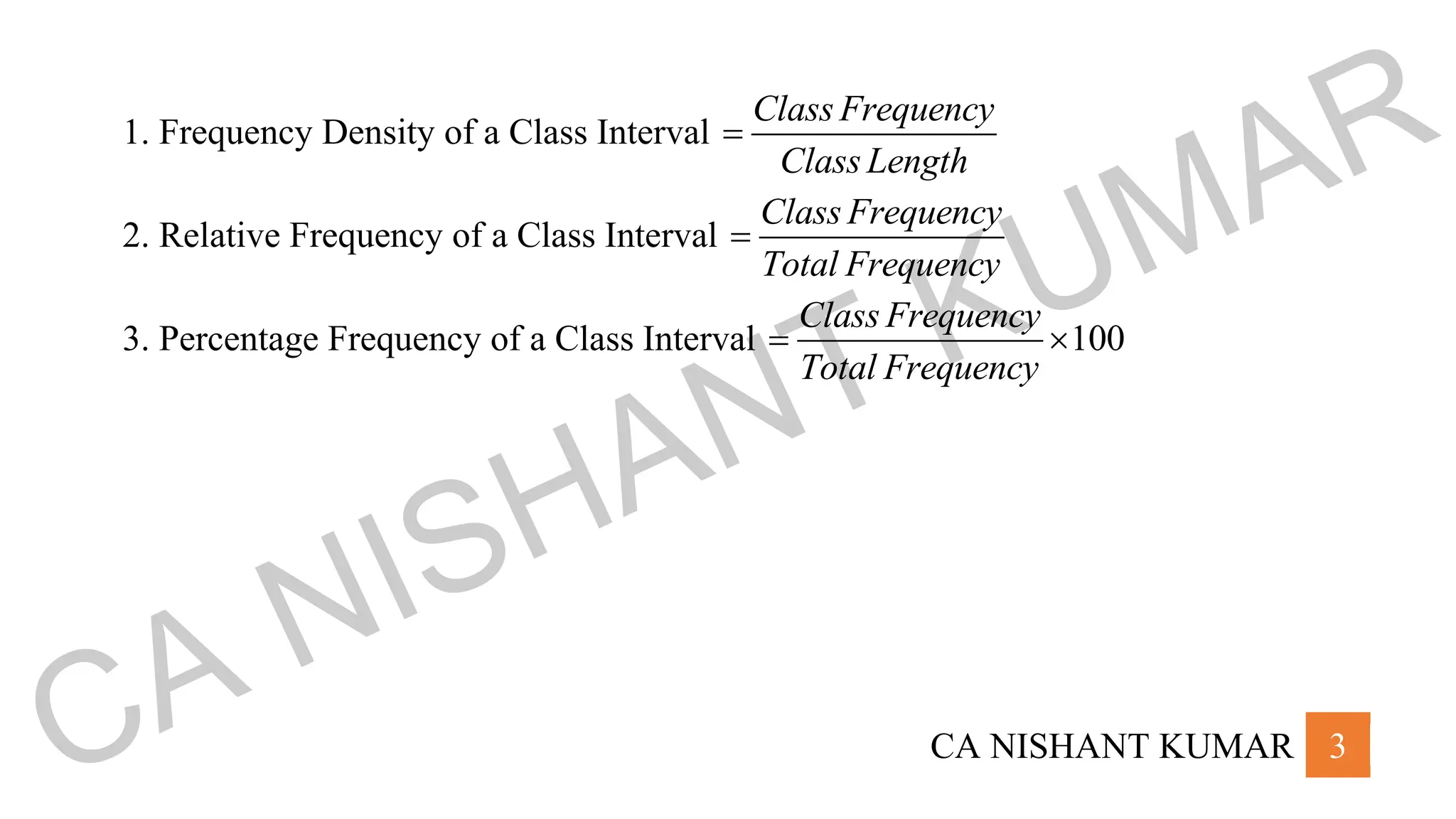
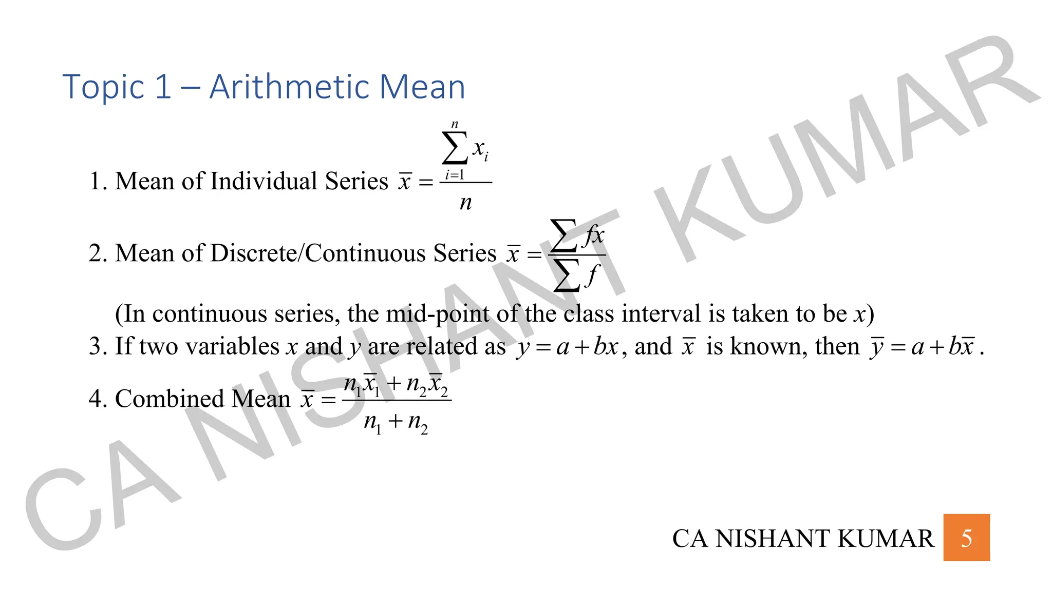
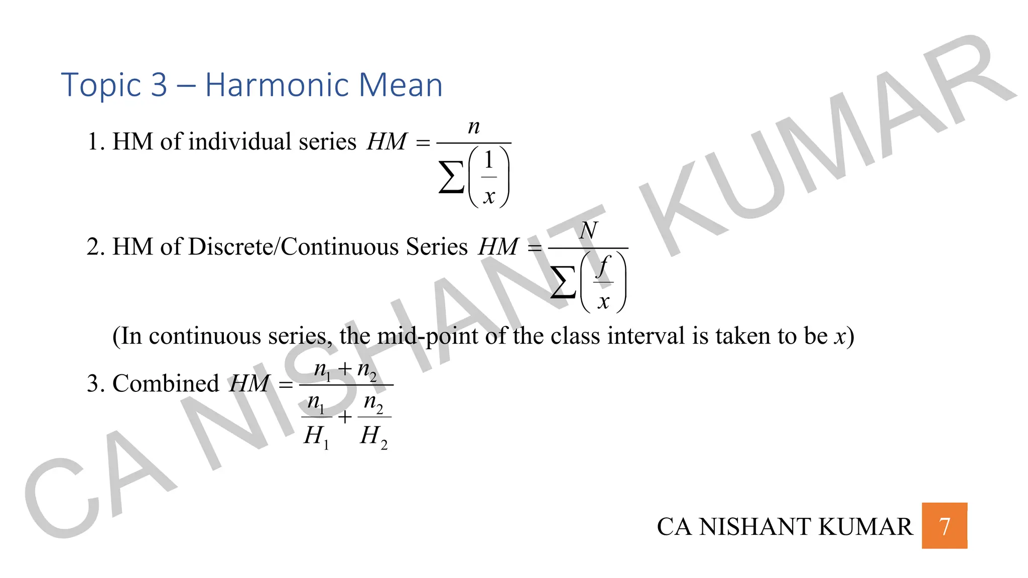
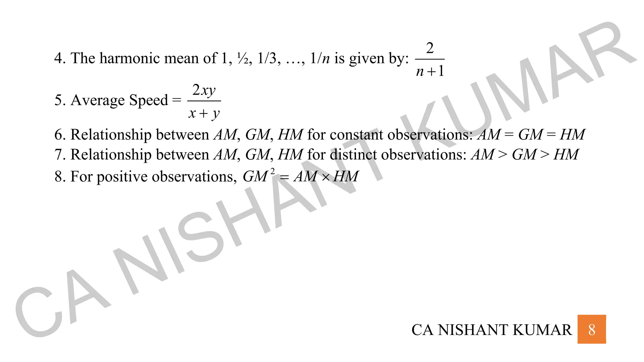
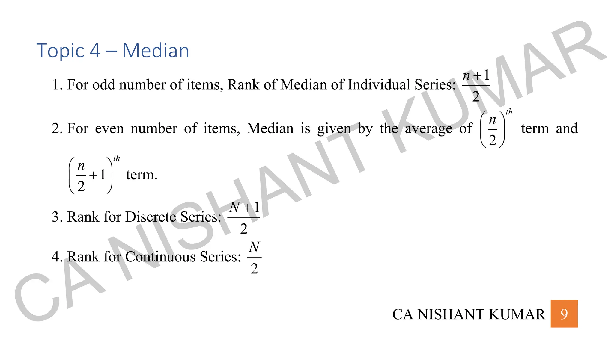
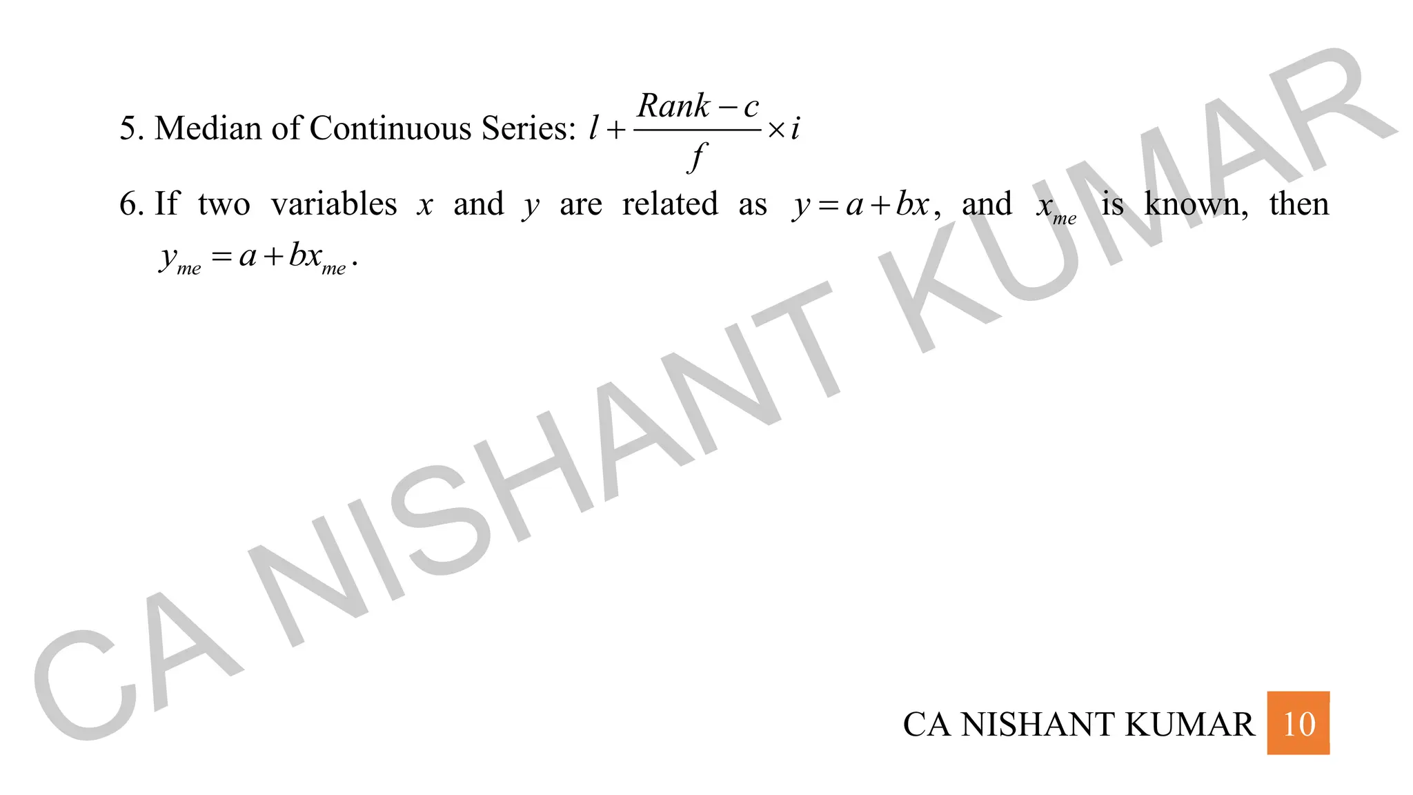
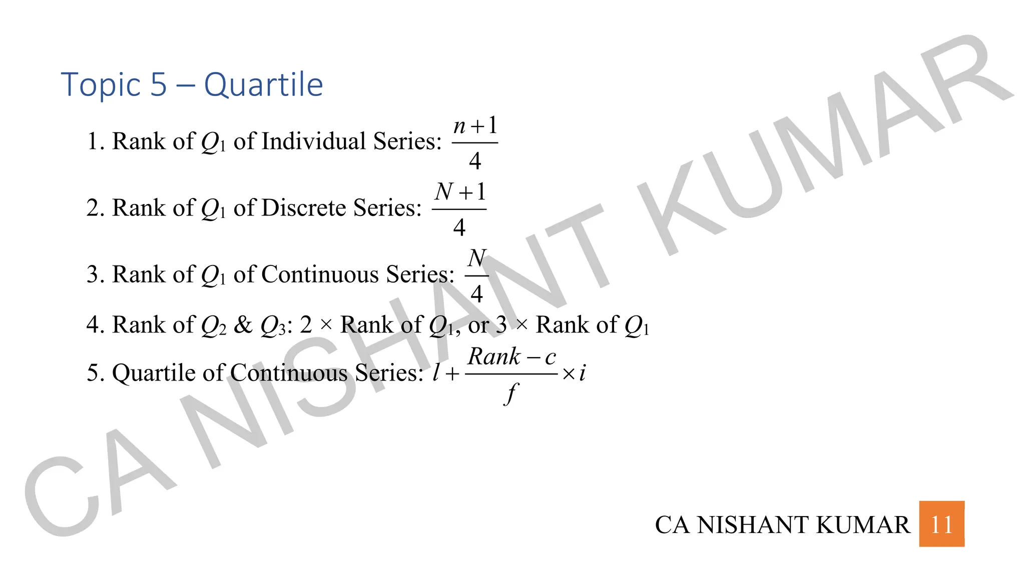
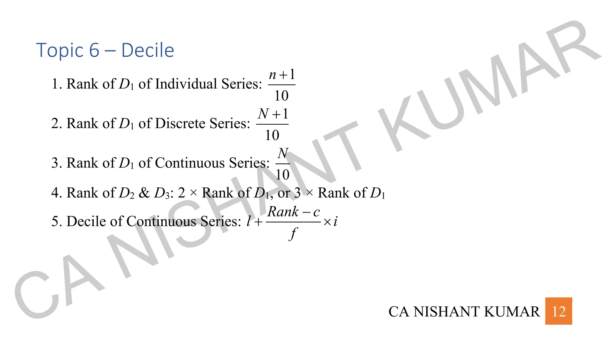
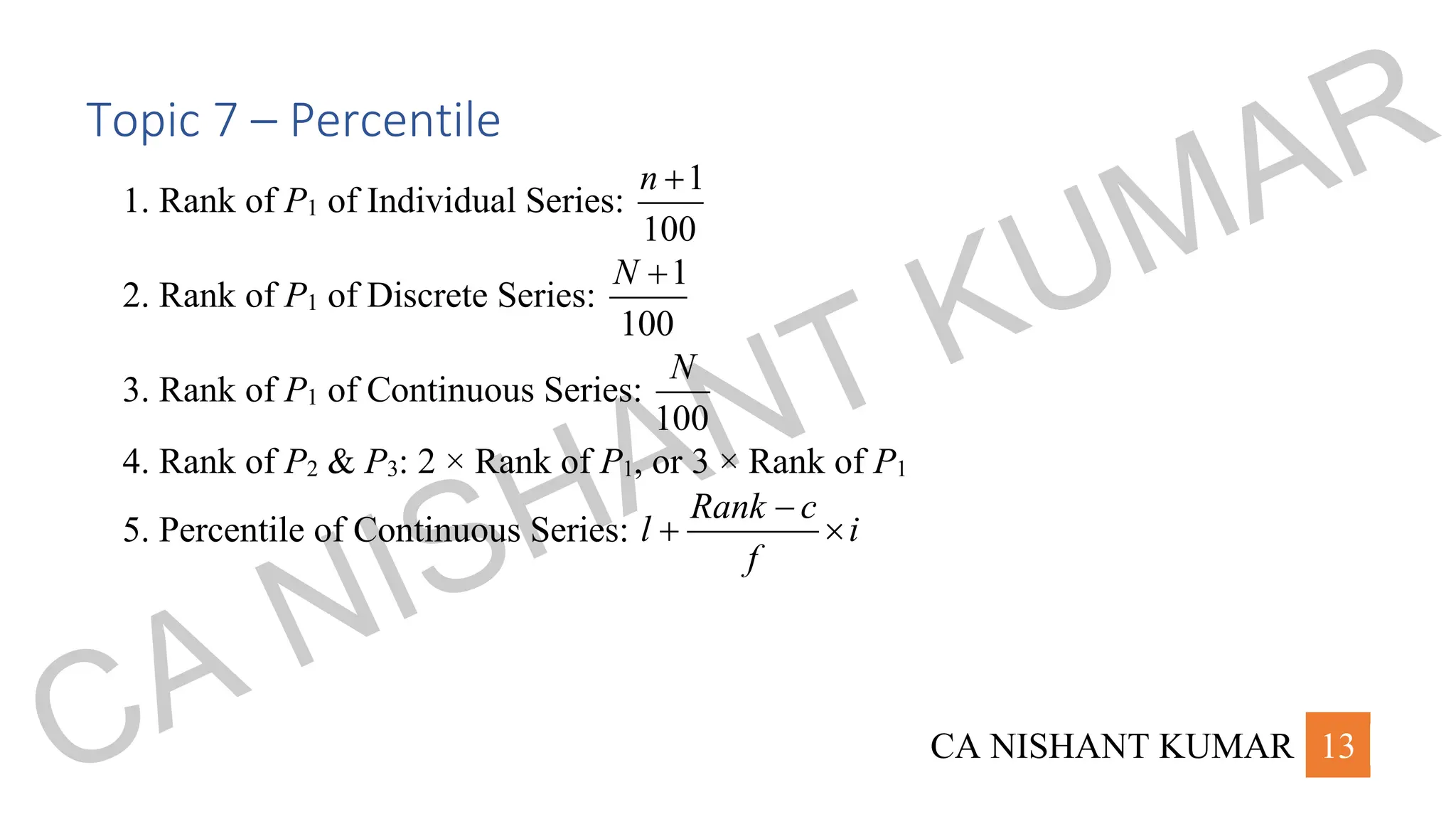
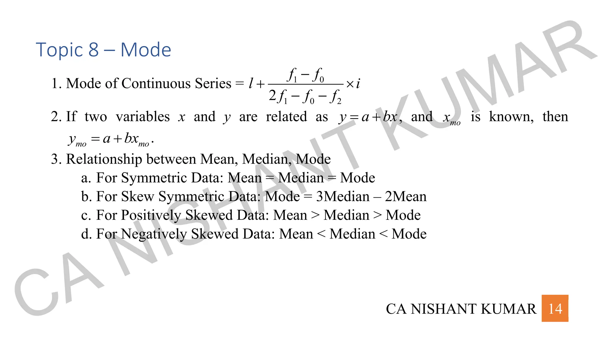
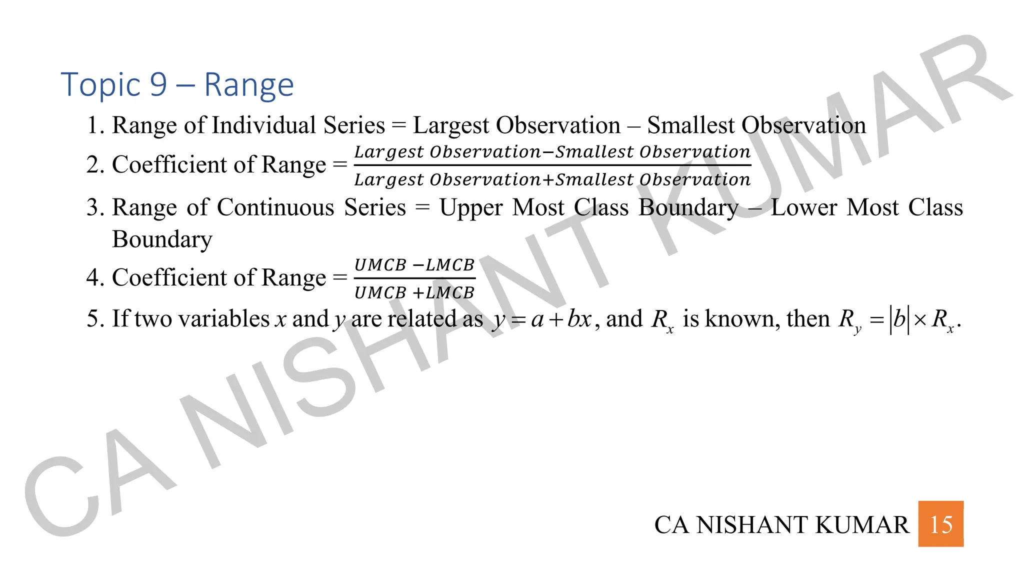
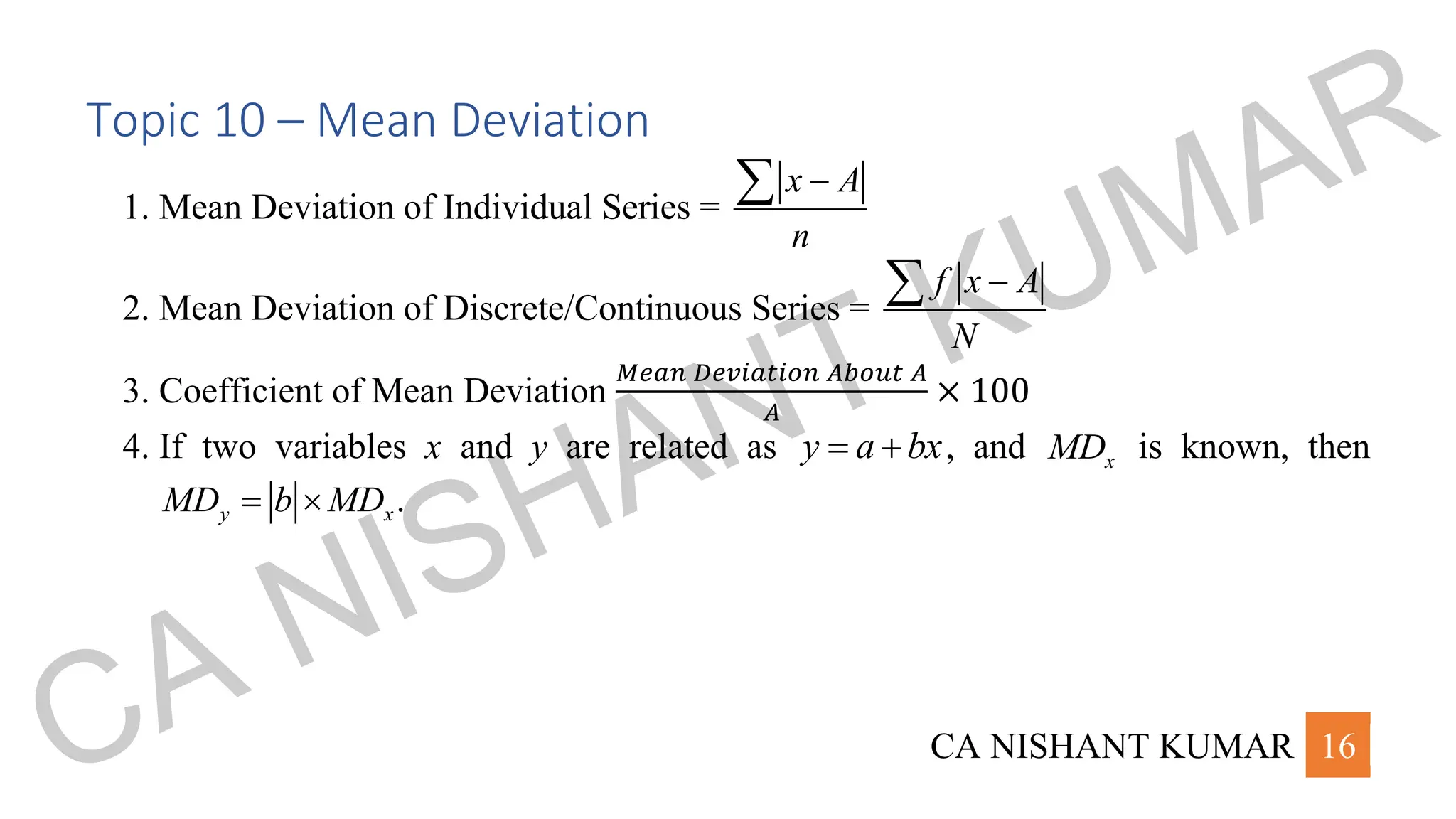
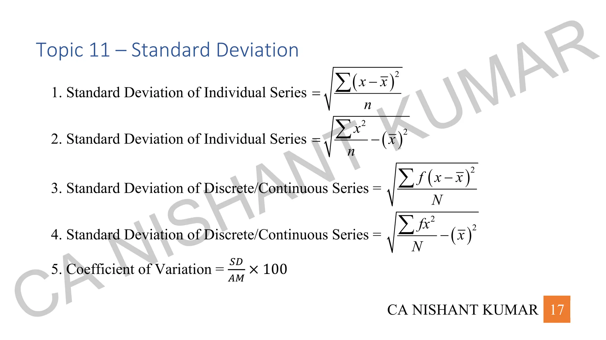
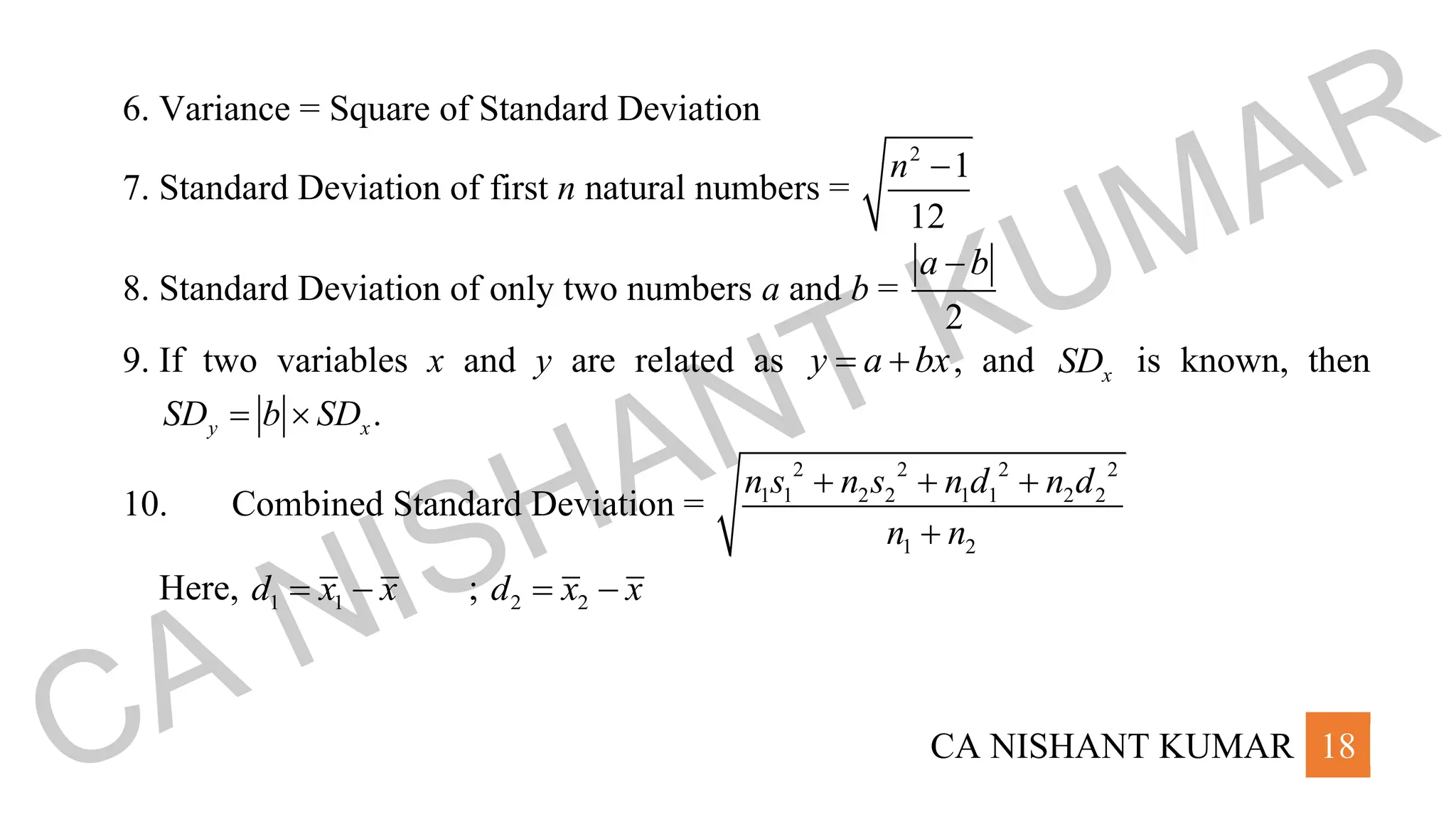
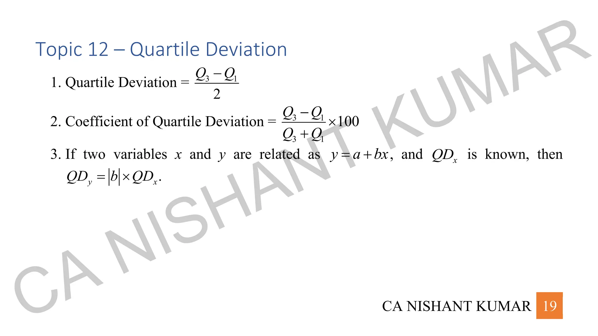
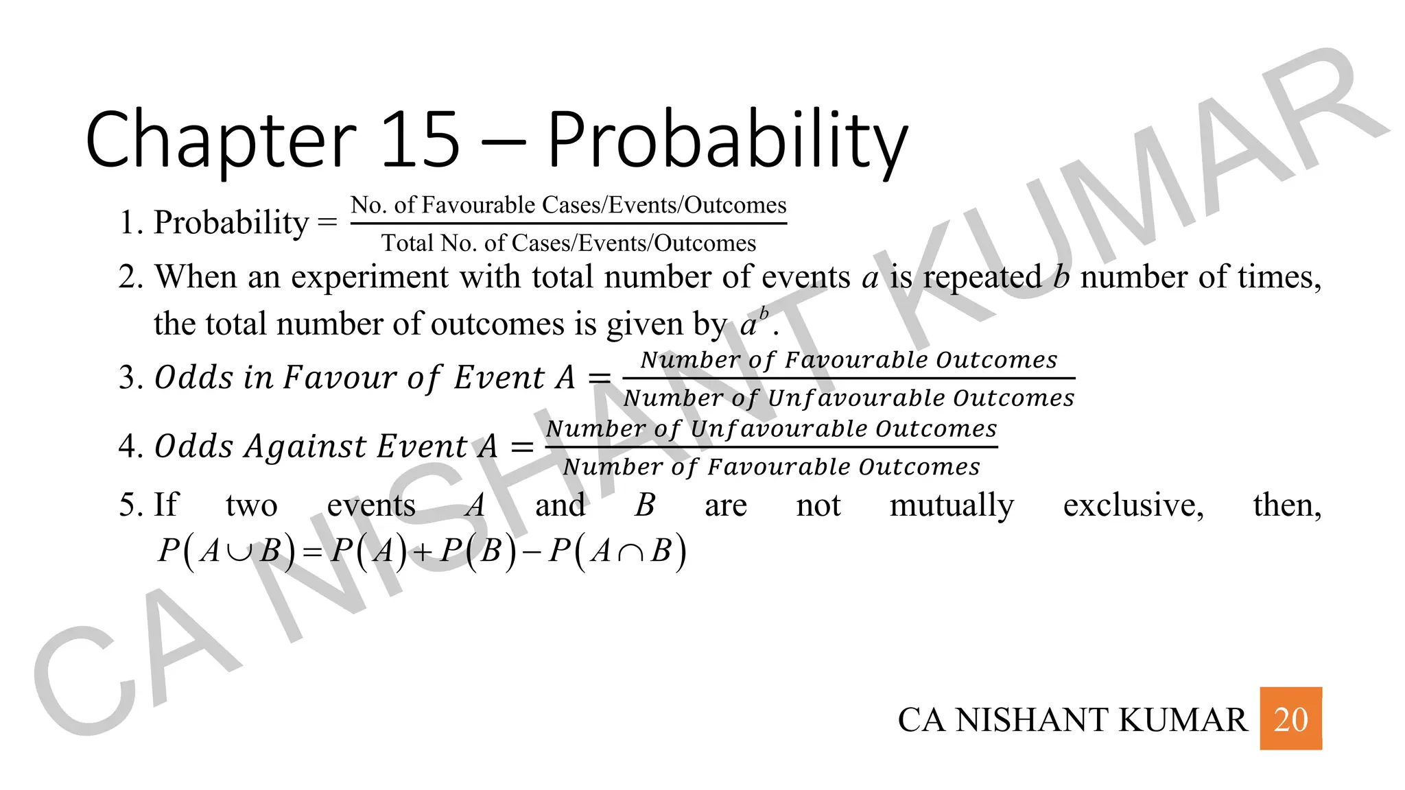
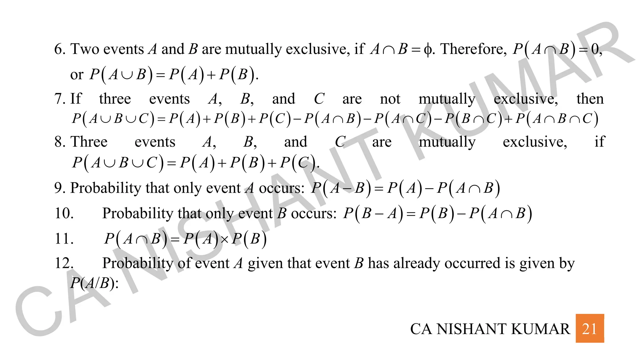
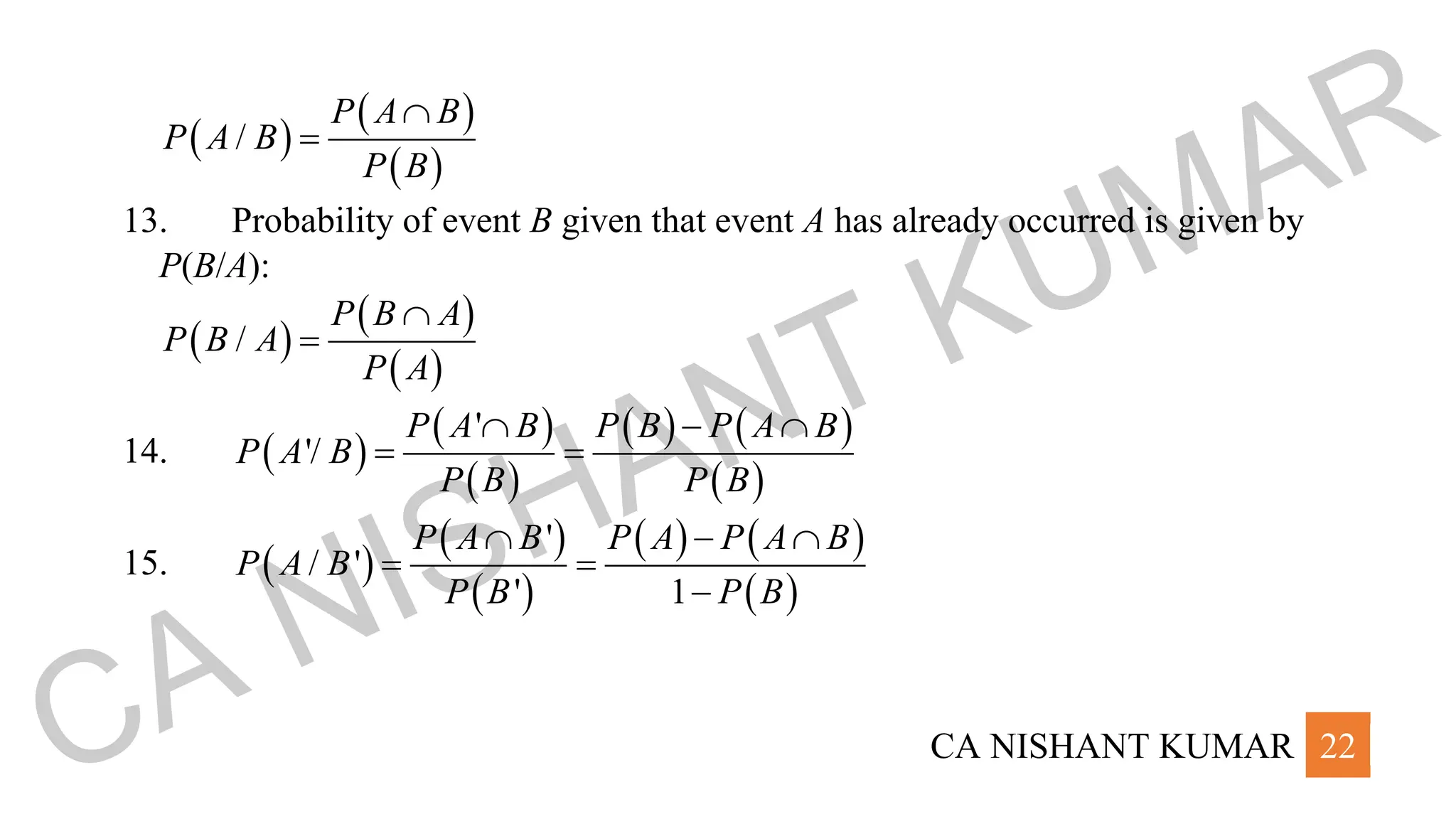
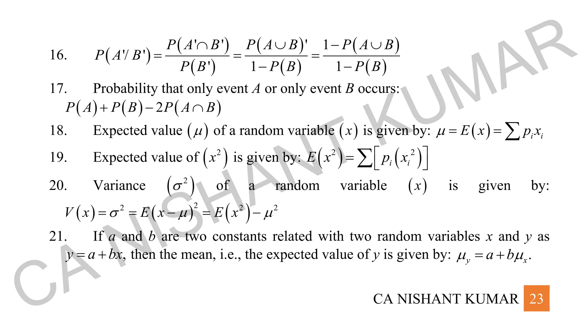
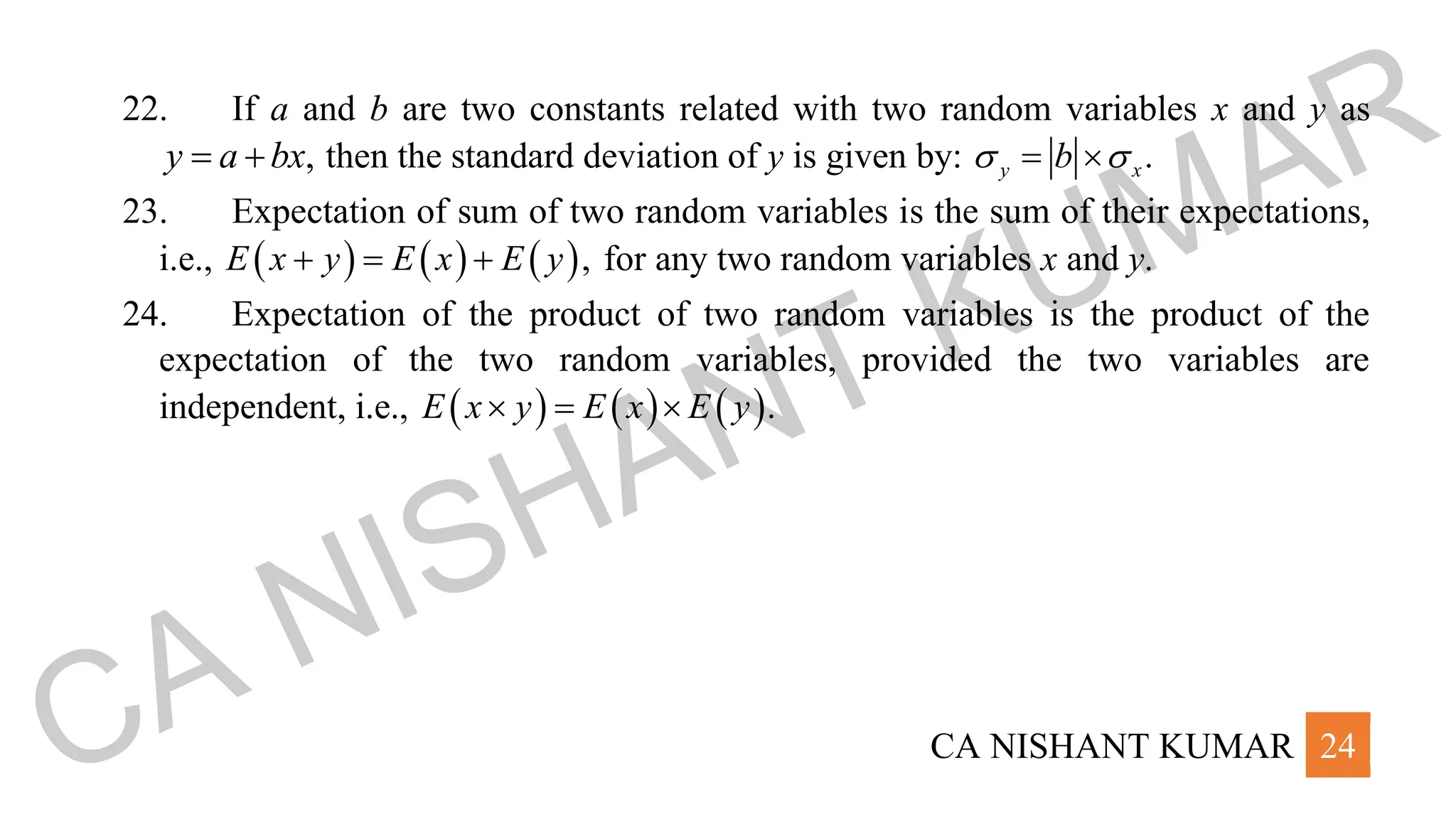
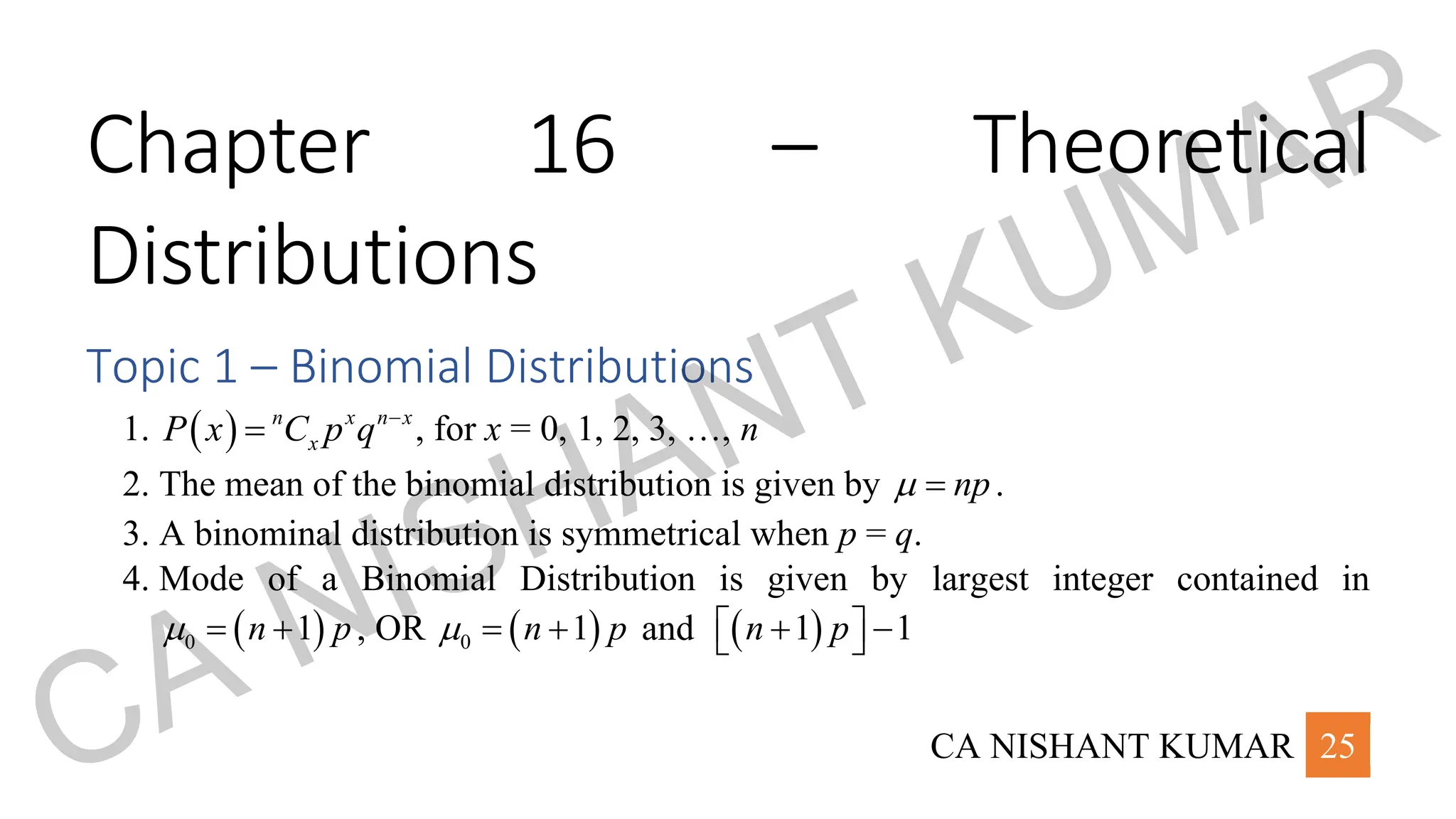
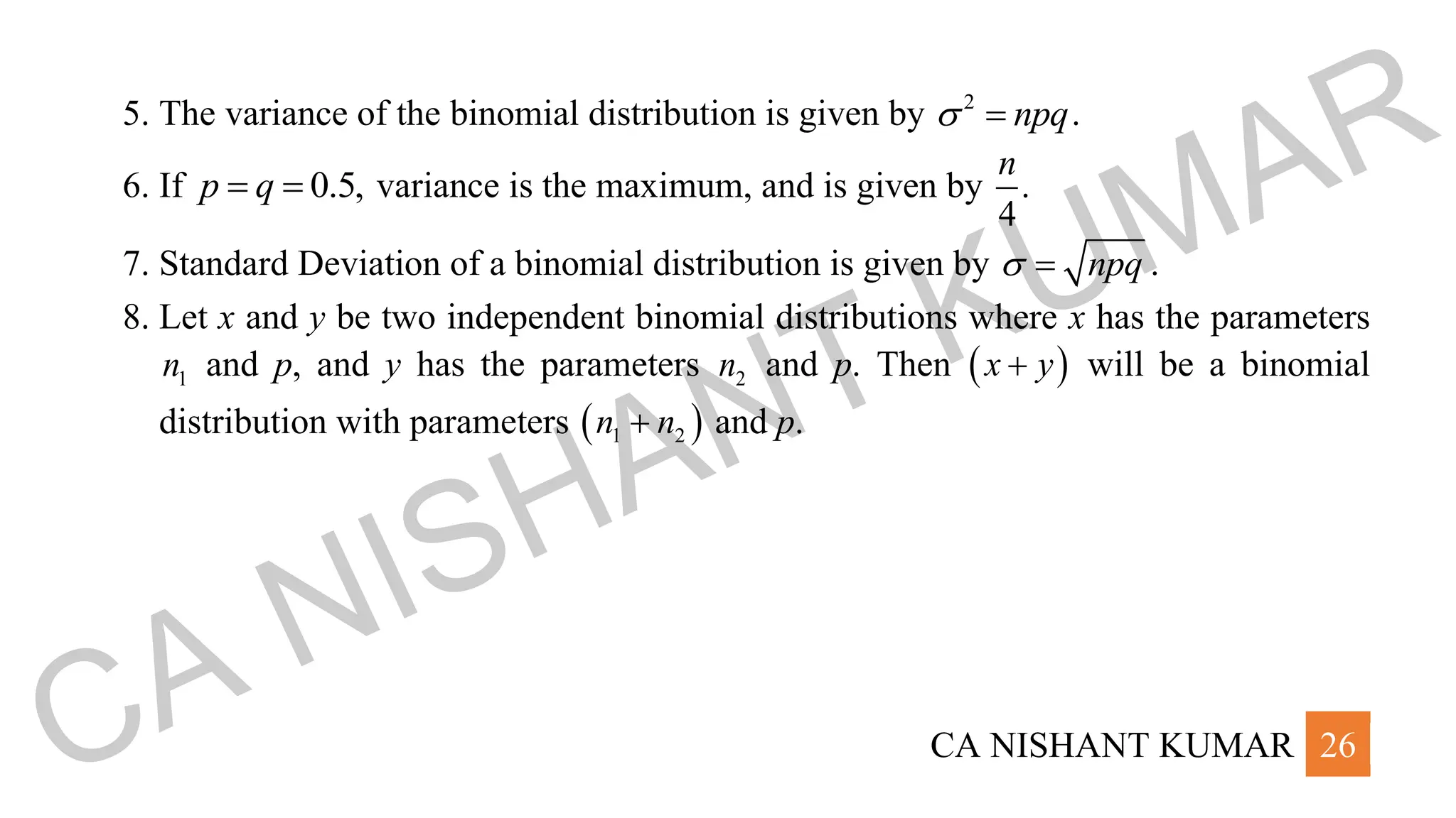
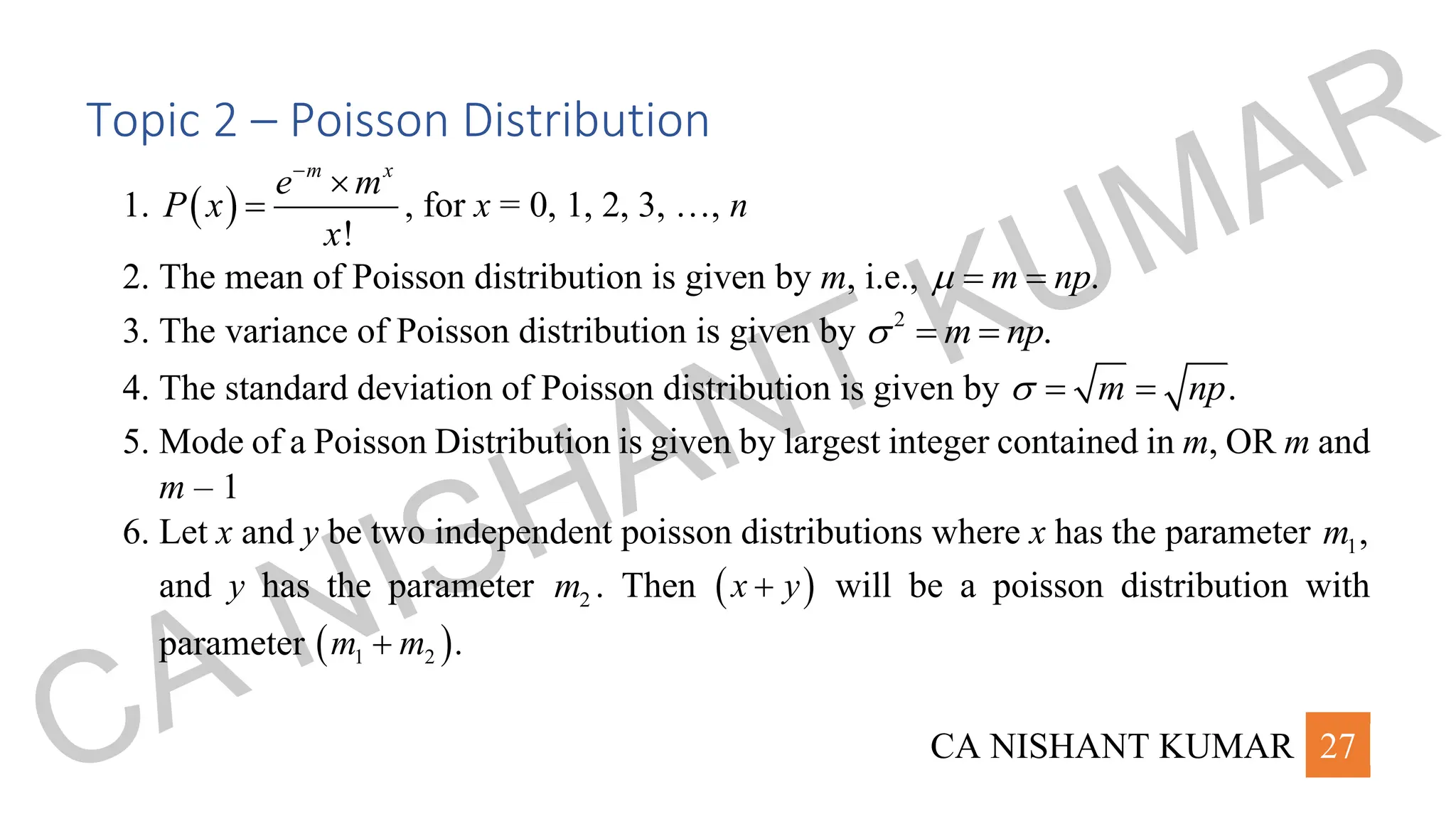
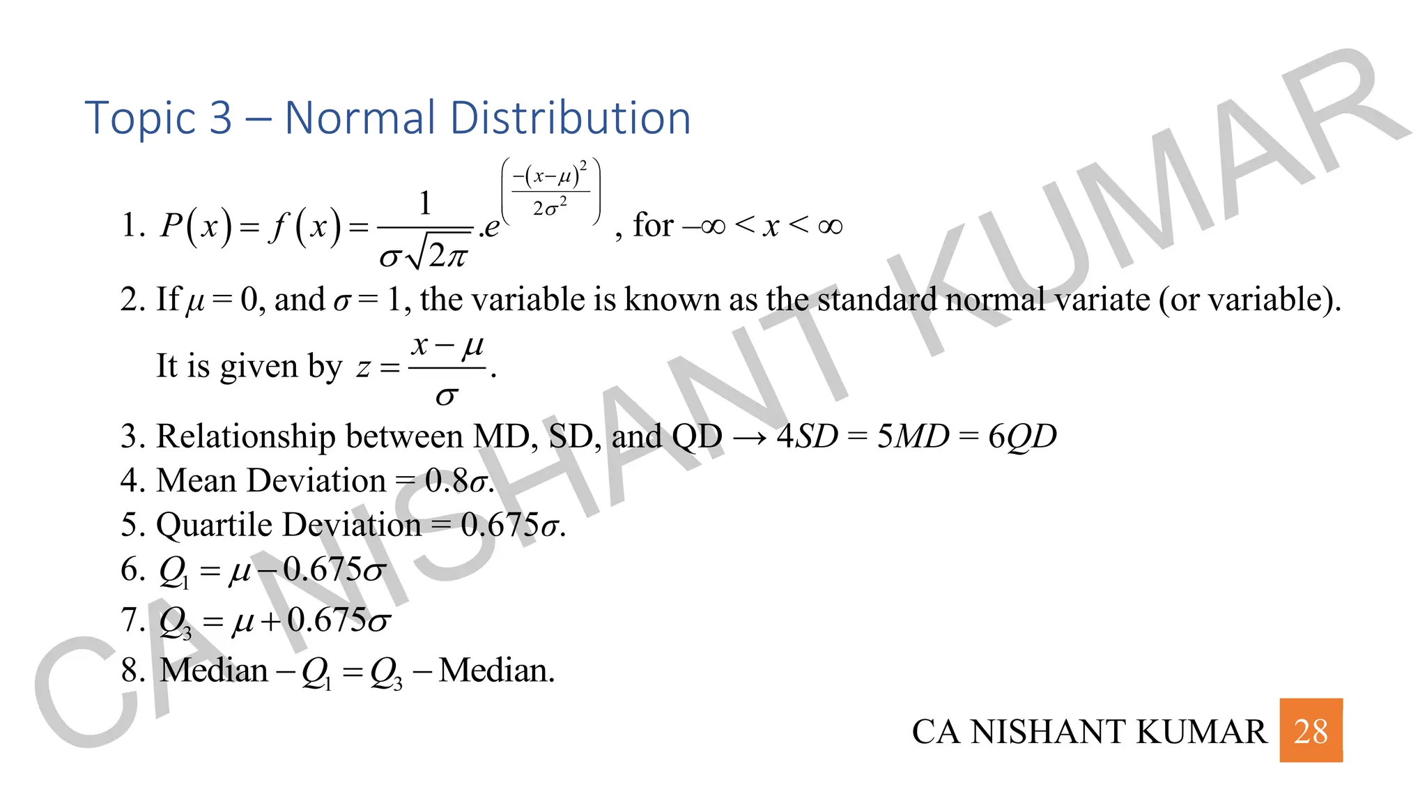
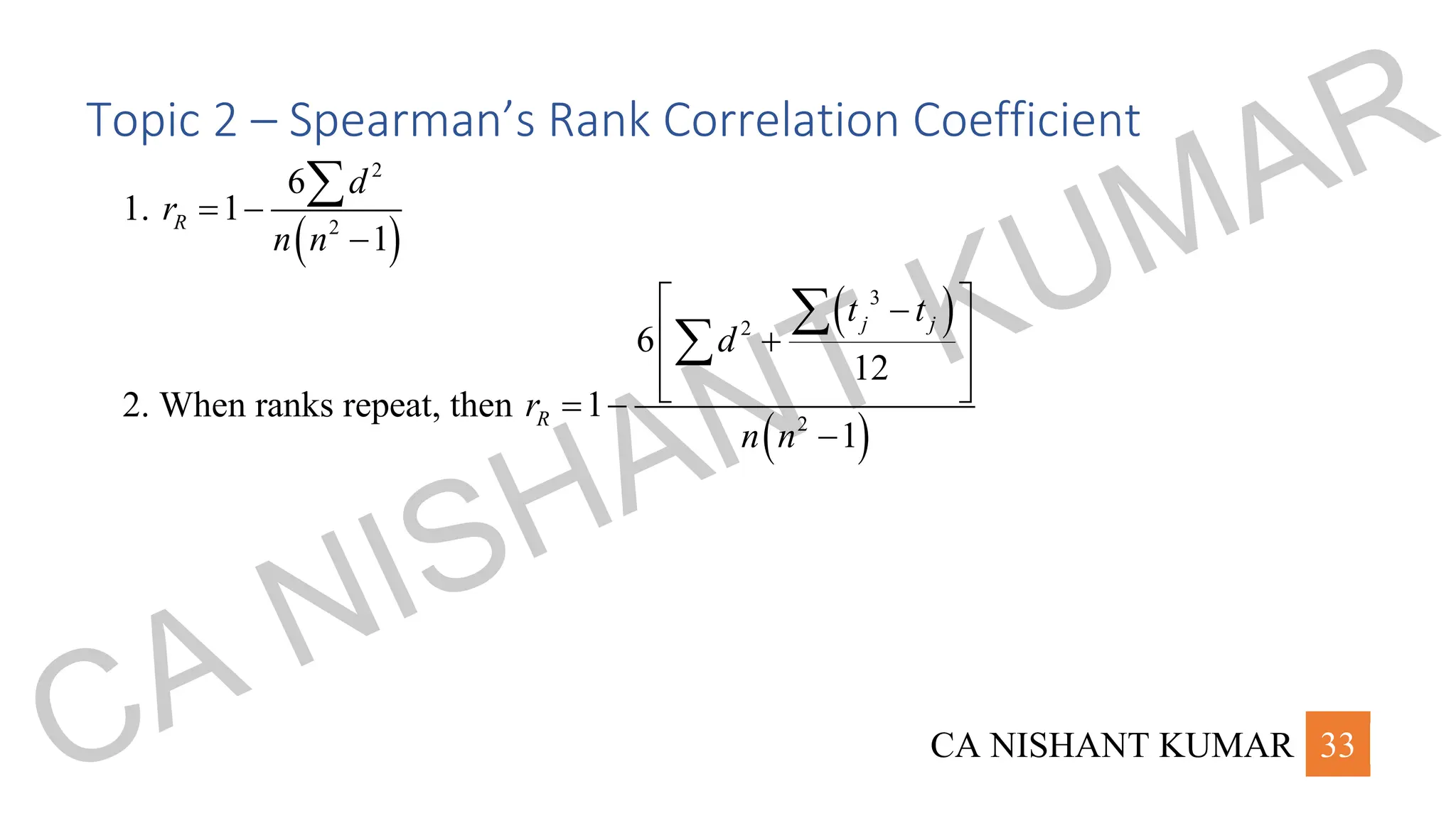
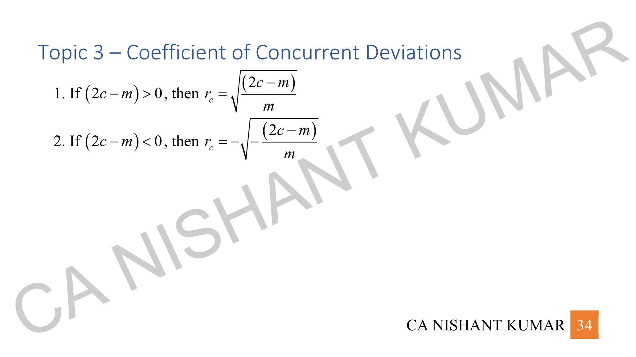
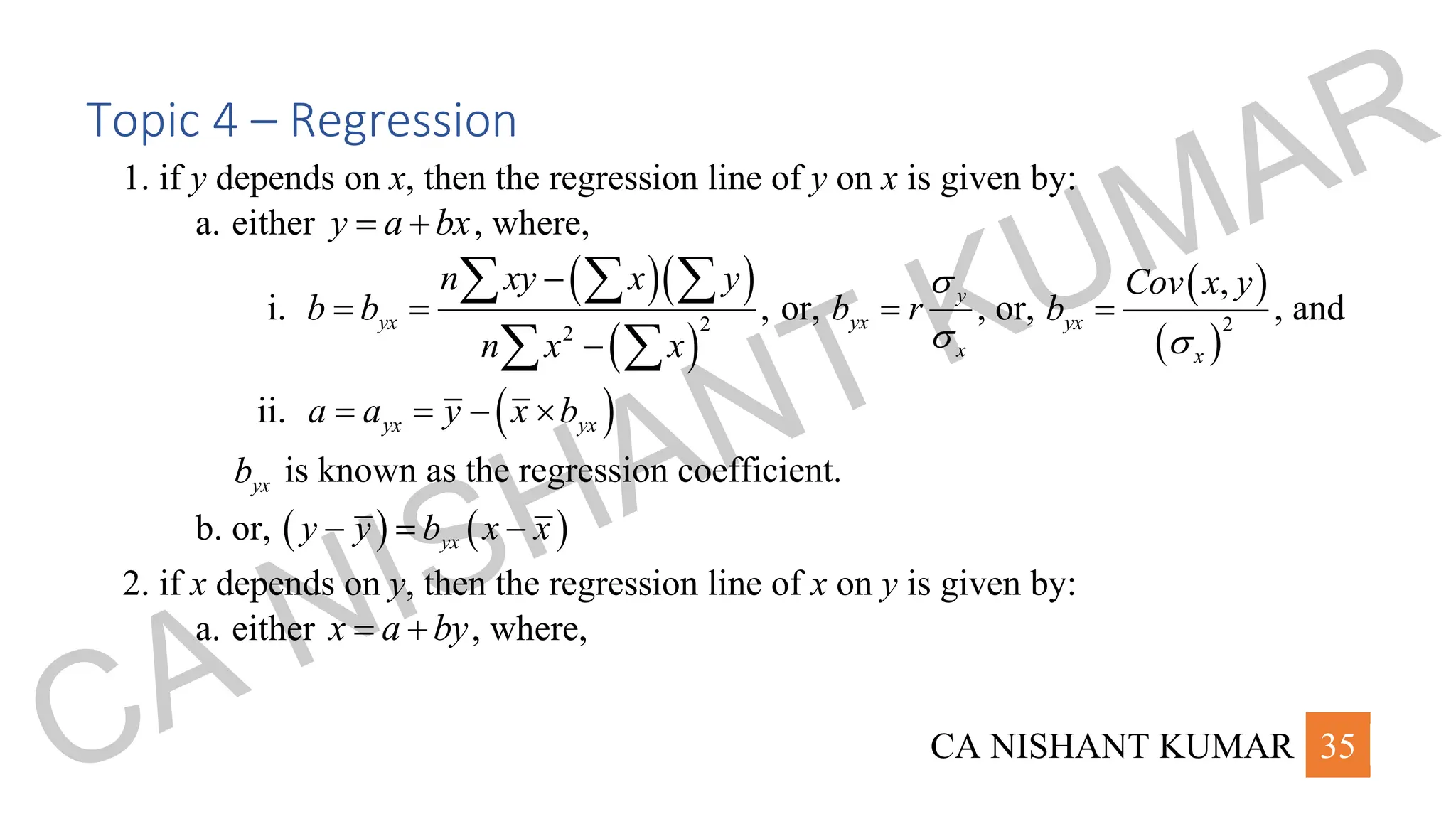
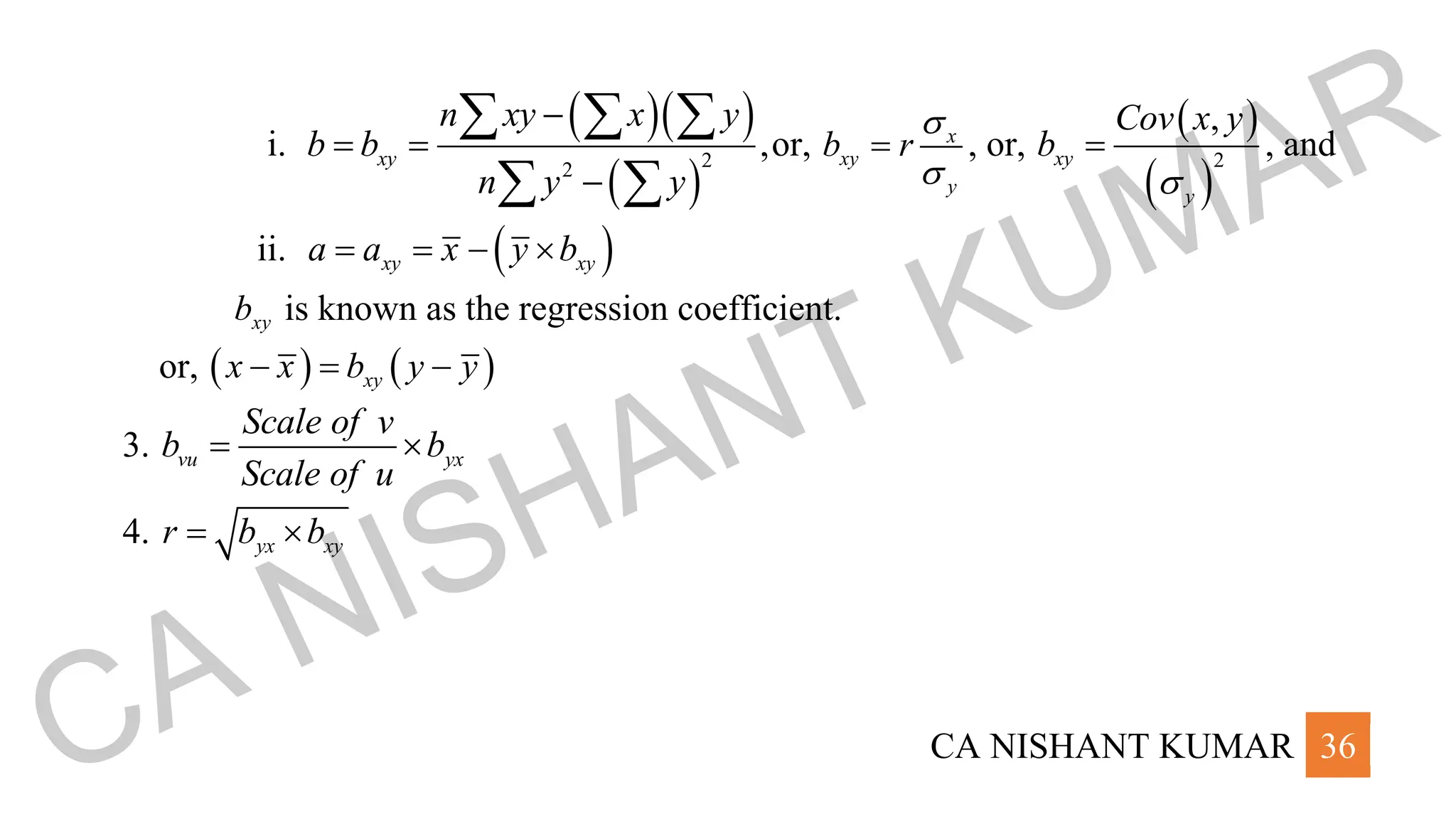
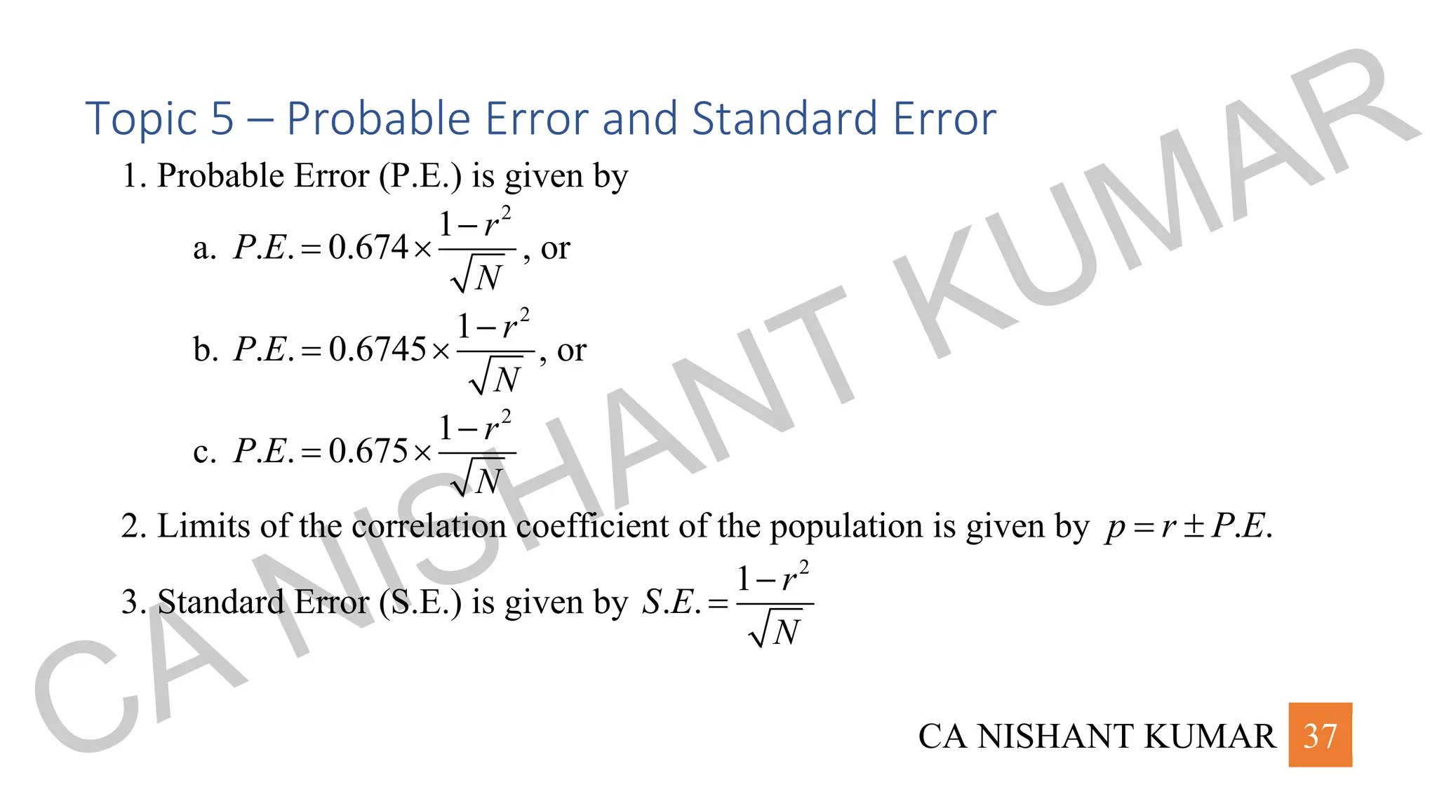
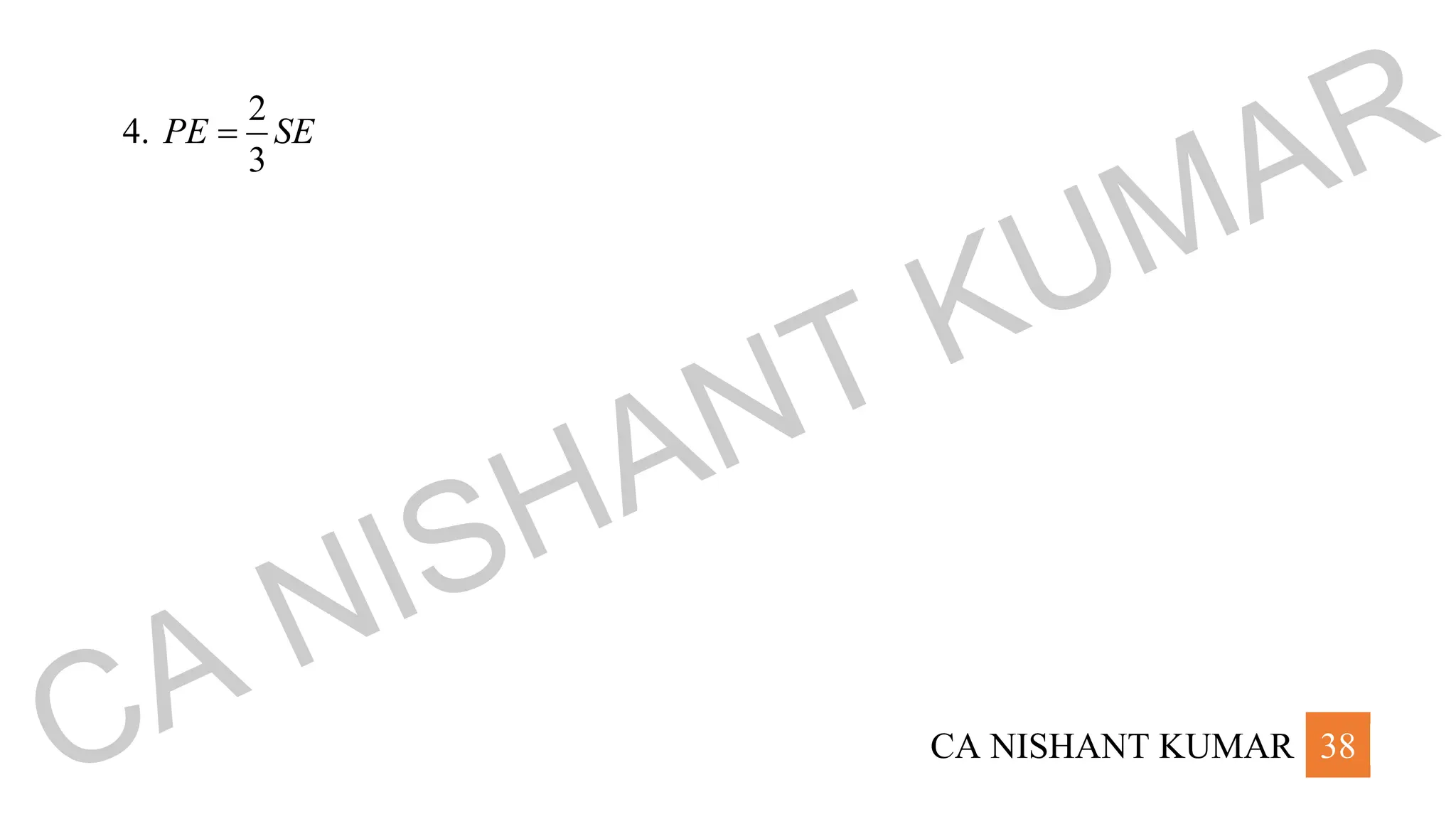
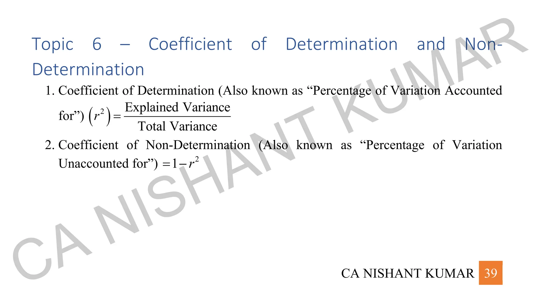
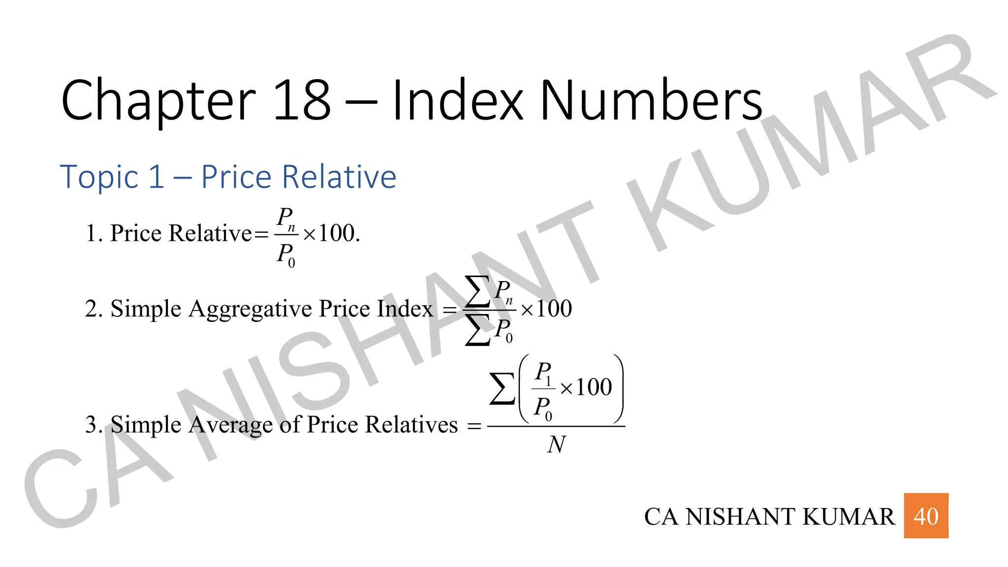
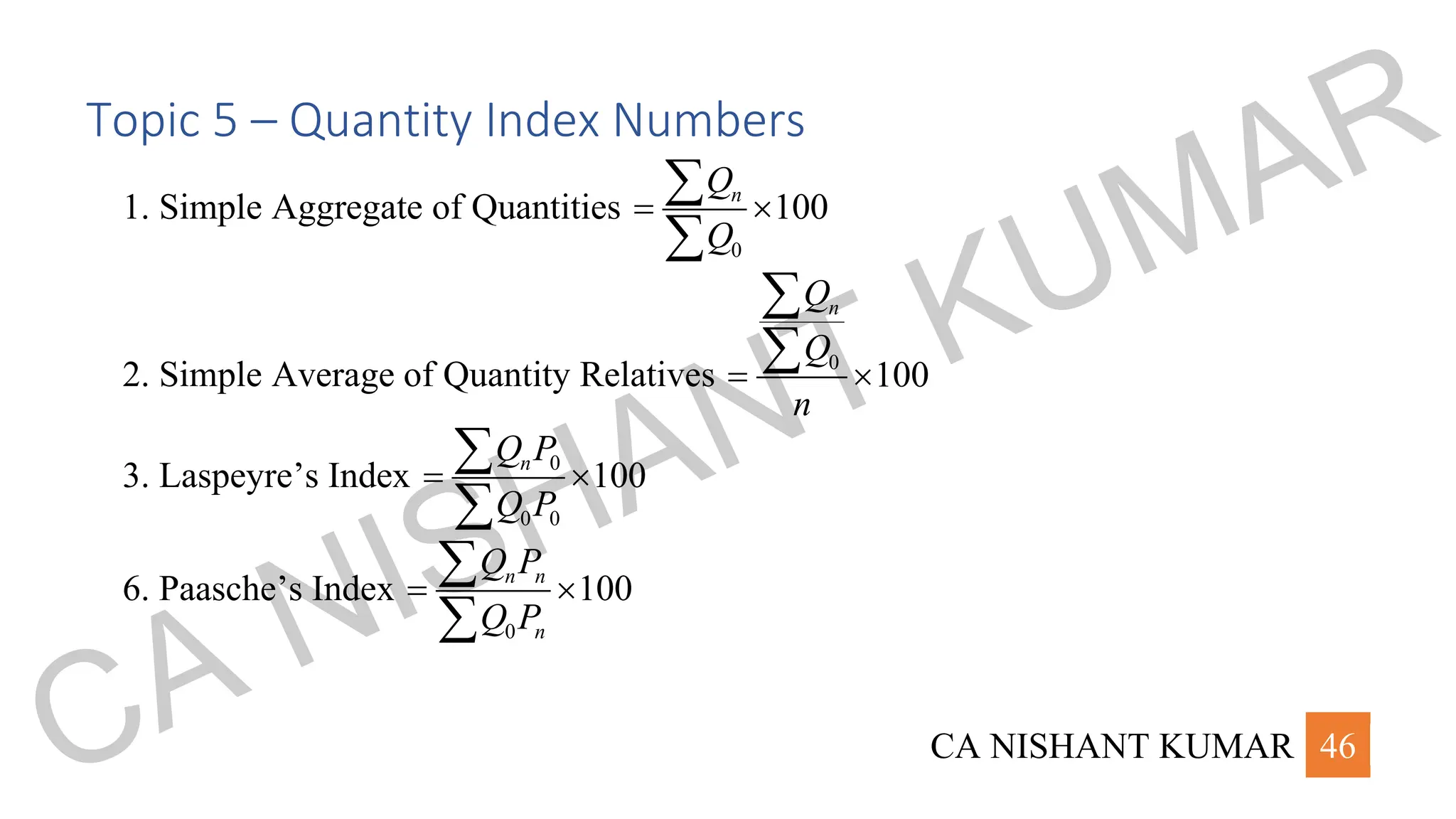
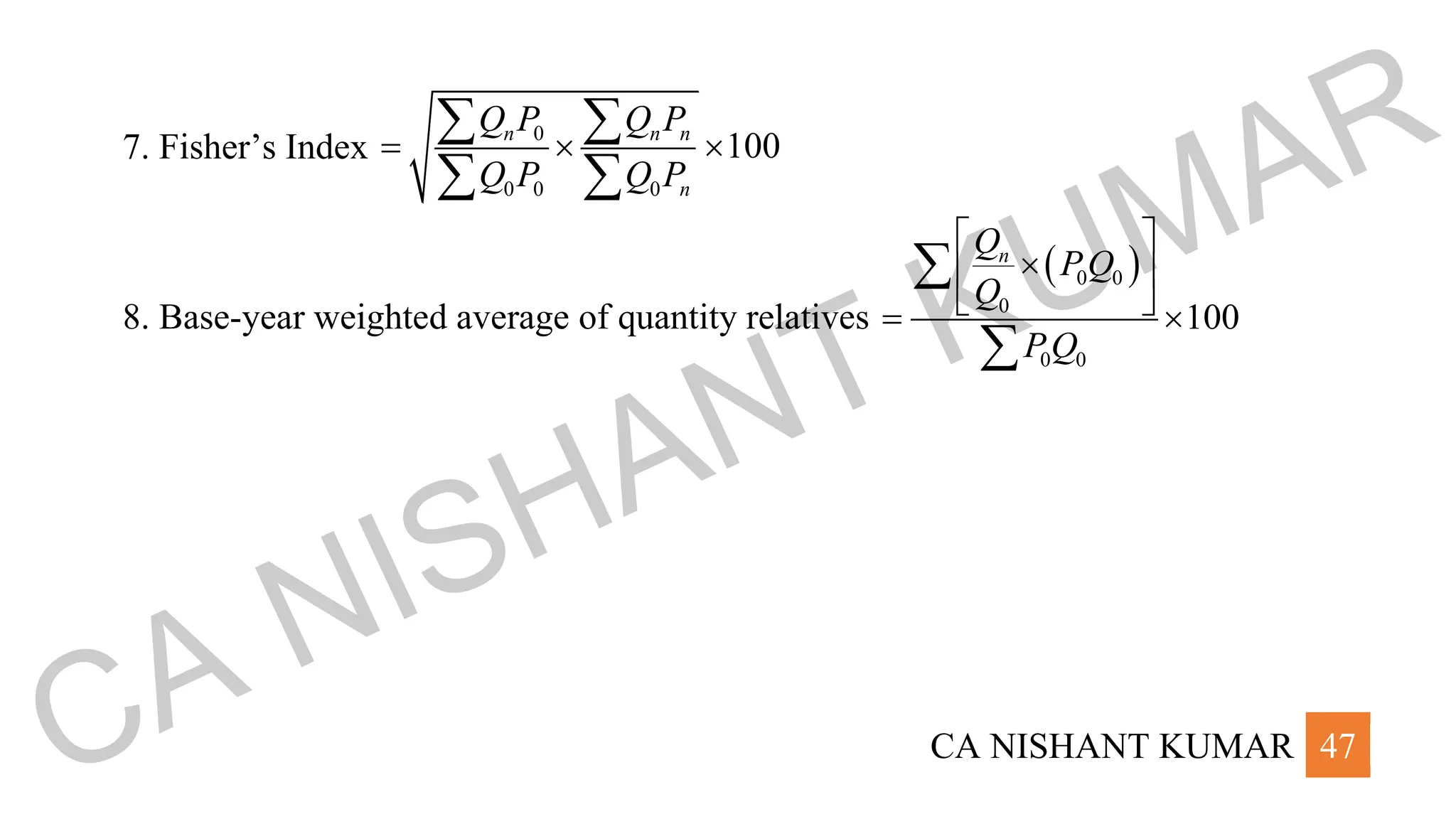
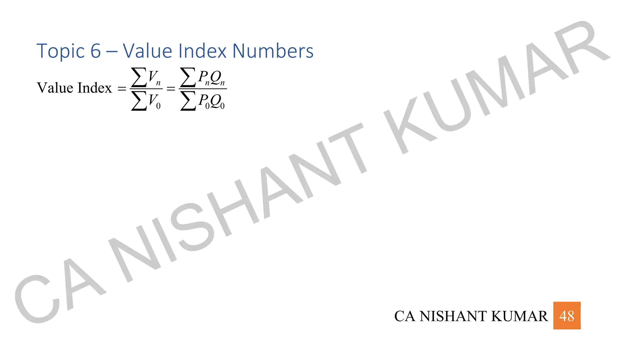
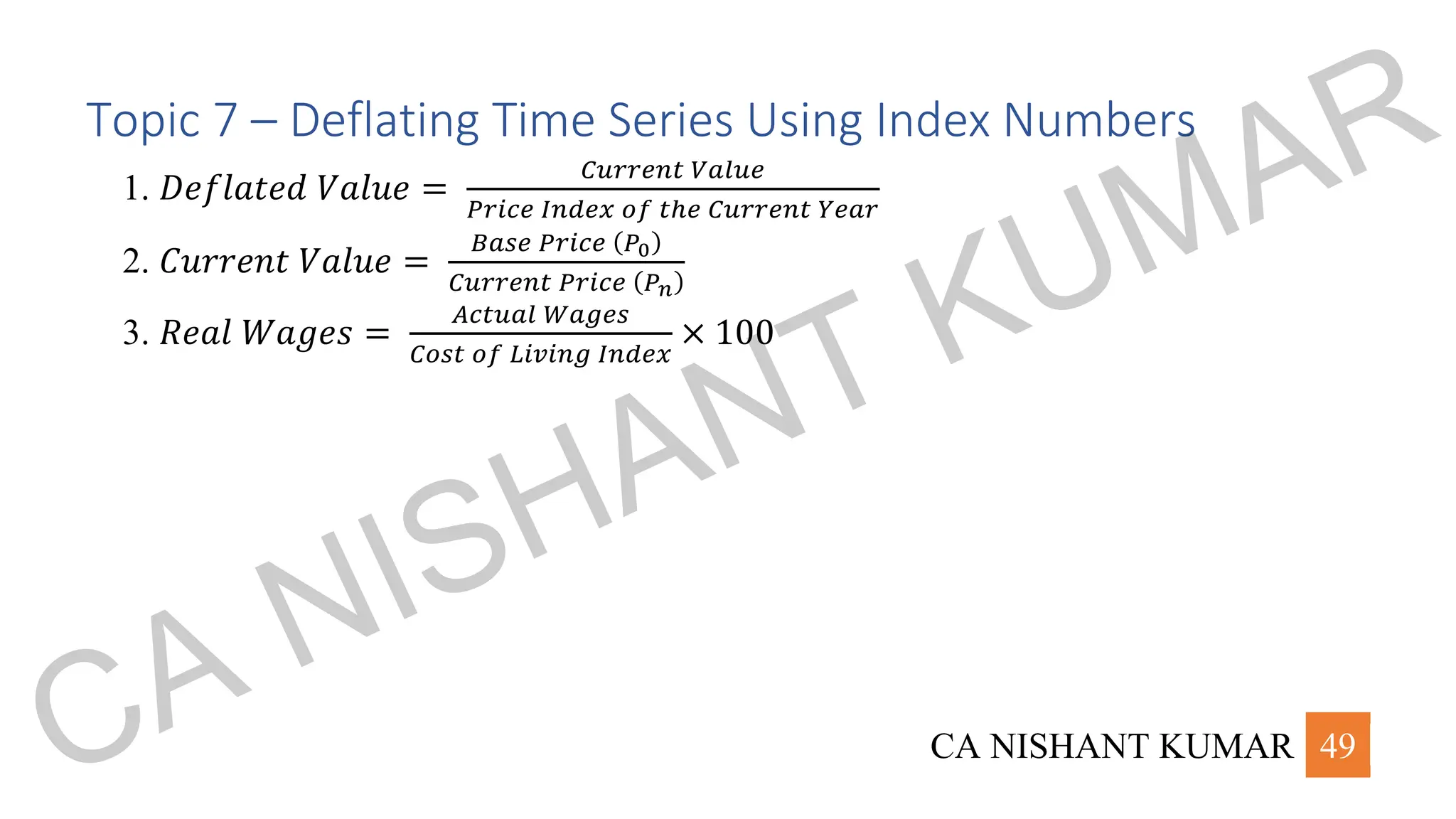
CA Nishant Kumar
STATISTICS FORMULA SHEET
CA NISHANT KUMAR
CA NISHANT KUMAR 1
Stay updated with the latest FREE lectures: https://www.youtube.com/@ekagrataca
CA NISHANT KUMAR
CA NISHANT KUMAR 2
Chapter 13 – Statistical Description
of Data
CA NISHANT KUMAR
CA NISHANT KUMAR 3
1. Frequency Density of a Class Interval
Class Frequency
Class Length
=
2. Relative Frequency of a Class Interval
Class Frequency
Total Frequency
=
3. Percentage Frequency of a Class Interval 100
Class Frequency
Total Frequency
= 
CA NISHANT KUMAR
CA NISHANT KUMAR 4
Chapter 14 – Measures of Central
Tendency and Dispersion
CA NISHANT KUMAR
CA NISHANT KUMAR 5
Topic 1 – Arithmetic Mean
1. Mean of Individual Series 1
n
i
i
x
x
n
=
=

2. Mean of Discrete/Continuous Series
fx
x
f
=


(In continuous series, the mid-point of the class interval is taken to be x)
3. If two variables x and y are related as y a bx
= + , and x is known, then y a bx
= + .
4. Combined Mean 1 1 2 2
1 2
n x n x
x
n n
+
=
+
CA NISHANT KUMAR
CA NISHANT KUMAR 6
Topic 2 – Geometric Mean
1. GM of Individual Series = nth
root of the product of n numbers
2. GM of Discrete/Continuous Series = ( )
1 2
1
1 2 ... n
f
f f N
n
x x x
  
(In continuous series, the mid-point of the class interval is taken to be x)
3. If z = xy, then GM of z = GM of x × GM of y
4. If
x
z
y
= , then
GM of x
GM of z
GM of y
=
5. For a set of r observations,
1
log log
G x
r
= 
CA NISHANT KUMAR
CA NISHANT KUMAR 7
Topic 3 – Harmonic Mean
1. HM of individual series
1
n
HM
x
=
 
 
 

2. HM of Discrete/Continuous Series
N
HM
f
x
=
 
 
 

(In continuous series, the mid-point of the class interval is taken to be x)
3. Combined 1 2
1 2
1 2
n n
HM
n n
H H
+
=
+
CA NISHANT KUMAR
CA NISHANT KUMAR 8
4. The harmonic mean of 1, ½, 1/3, …, 1/n is given by:
2
1
n +
5. Average Speed =
2xy
x y
+
6. Relationship between AM, GM, HM for constant observations: AM = GM = HM
7. Relationship between AM, GM, HM for distinct observations: AM > GM > HM
8. For positive observations, 2
GM AM HM
= 
CA NISHANT KUMAR
CA NISHANT KUMAR 9
Topic 4 – Median
1. For odd number of items, Rank of Median of Individual Series:
1
2
n +
2. For even number of items, Median is given by the average of
2
th
n
 
 
 
term and
1
2
th
n
 
+
 
 
term.
3. Rank for Discrete Series:
1
2
N +
4. Rank for Continuous Series:
2
N
CA NISHANT KUMAR
CA NISHANT KUMAR 10
5. Median of Continuous Series:
Rank c
l i
f
−
+ 
6. If two variables x and y are related as y a bx
= + , and me
x is known, then
me me
y a bx
= + .
CA NISHANT KUMAR
CA NISHANT KUMAR 11
Topic 5 – Quartile
1. Rank of Q1 of Individual Series:
1
4
n +
2. Rank of Q1 of Discrete Series:
1
4
N +
3. Rank of Q1 of Continuous Series:
4
N
4. Rank of Q2 & Q3: 2 × Rank of Q1, or 3 × Rank of Q1
5. Quartile of Continuous Series:
Rank c
l i
f
−
+ 
CA NISHANT KUMAR
CA NISHANT KUMAR 12
Topic 6 – Decile
1. Rank of D1 of Individual Series:
1
10
n +
2. Rank of D1 of Discrete Series:
1
10
N +
3. Rank of D1 of Continuous Series:
10
N
4. Rank of D2 & D3: 2 × Rank of D1, or 3 × Rank of D1
5. Decile of Continuous Series:
Rank c
l i
f
−
+ 
CA NISHANT KUMAR
CA NISHANT KUMAR 13
Topic 7 – Percentile
1. Rank of P1 of Individual Series:
1
100
n +
2. Rank of P1 of Discrete Series:
1
100
N +
3. Rank of P1 of Continuous Series:
100
N
4. Rank of P2 & P3: 2 × Rank of P1, or 3 × Rank of P1
5. Percentile of Continuous Series:
Rank c
l i
f
−
+ 
CA NISHANT KUMAR
CA NISHANT KUMAR 14
Topic 8 – Mode
1. Mode of Continuous Series = 1 0
1 0 2
2
f f
l i
f f f
−
+ 
− −
2. If two variables x and y are related as y a bx
= + , and mo
x is known, then
mo mo
y a bx
= + .
3. Relationship between Mean, Median, Mode
a. For Symmetric Data: Mean = Median = Mode
b. For Skew Symmetric Data: Mode = 3Median – 2Mean
c. For Positively Skewed Data: Mean > Median > Mode
d. For Negatively Skewed Data: Mean < Median < Mode
CA NISHANT KUMAR
CA NISHANT KUMAR 15
Topic 9 – Range
1. Range of Individual Series = Largest Observation – Smallest Observation
2. Coefficient of Range =
𝐿𝑎𝑟𝑔𝑒𝑠𝑡 𝑂𝑏𝑠𝑒𝑟𝑣𝑎𝑡𝑖𝑜𝑛−𝑆𝑚𝑎𝑙𝑙𝑒𝑠𝑡 𝑂𝑏𝑠𝑒𝑟𝑣𝑎𝑡𝑖𝑜𝑛
𝐿𝑎𝑟𝑔𝑒𝑠𝑡 𝑂𝑏𝑠𝑒𝑟𝑣𝑎𝑡𝑖𝑜𝑛+𝑆𝑚𝑎𝑙𝑙𝑒𝑠𝑡 𝑂𝑏𝑠𝑒𝑟𝑣𝑎𝑡𝑖𝑜𝑛
3. Range of Continuous Series = Upper Most Class Boundary – Lower Most Class
Boundary
4. Coefficient of Range =
𝑈𝑀𝐶𝐵 −𝐿𝑀𝐶𝐵
𝑈𝑀𝐶𝐵 +𝐿𝑀𝐶𝐵
5. If two variables x and y are related as y a bx
= + , and x
R is known, then .
y x
R b R
= 
CA NISHANT KUMAR
CA NISHANT KUMAR 16
Topic 10 – Mean Deviation
1. Mean Deviation of Individual Series =
x A
n
−

2. Mean Deviation of Discrete/Continuous Series =
f x A
N
−

3. Coefficient of Mean Deviation
𝑀𝑒𝑎𝑛 𝐷𝑒𝑣𝑖𝑎𝑡𝑖𝑜𝑛 𝐴𝑏𝑜𝑢𝑡 𝐴
𝐴
× 100
4. If two variables x and y are related as y a bx
= + , and x
MD is known, then
.
y x
MD b MD
= 
CA NISHANT KUMAR
CA NISHANT KUMAR 17
Topic 11 – Standard Deviation
1. Standard Deviation of Individual Series
( )
2
x x
n
−
=

2. Standard Deviation of Individual Series ( )
2
2
x
x
n
= −

3. Standard Deviation of Discrete/Continuous Series =
( )
2
f x x
N
−

4. Standard Deviation of Discrete/Continuous Series = ( )
2
2
fx
x
N
−

5. Coefficient of Variation =
𝑆𝐷
𝐴𝑀
× 100
CA NISHANT KUMAR
CA NISHANT KUMAR 18
6. Variance = Square of Standard Deviation
7. Standard Deviation of first n natural numbers =
2
1
12
n −
8. Standard Deviation of only two numbers a and b =
2
a b
−
9. If two variables x and y are related as y a bx
= + , and x
SD is known, then
.
y x
SD b SD
= 
10. Combined Standard Deviation =
2 2 2 2
1 1 2 2 1 1 2 2
1 2
n s n s n d n d
n n
+ + +
+
Here, 1 1
d x x
= − ; 2 2
d x x
= −
CA NISHANT KUMAR
CA NISHANT KUMAR 19
Topic 12 – Quartile Deviation
1. Quartile Deviation = 3 1
2
Q Q
−
2. Coefficient of Quartile Deviation = 3 1
3 1
100
Q Q
Q Q
−

+
3. If two variables x and y are related as y a bx
= + , and x
QD is known, then
.
y x
QD b QD
= 
CA NISHANT KUMAR
CA NISHANT KUMAR 20
Chapter 15 – Probability
1. Probability =
No. of Favourable Cases/Events/Outcomes
Total No. of Cases/Events/Outcomes
2. When an experiment with total number of events a is repeated b number of times,
the total number of outcomes is given by .
b
a
3. 𝑂𝑑𝑑𝑠 𝑖𝑛 𝐹𝑎𝑣𝑜𝑢𝑟 𝑜𝑓 𝐸𝑣𝑒𝑛𝑡 𝐴 =
𝑁𝑢𝑚𝑏𝑒𝑟 𝑜𝑓 𝐹𝑎𝑣𝑜𝑢𝑟𝑎𝑏𝑙𝑒 𝑂𝑢𝑡𝑐𝑜𝑚𝑒𝑠
𝑁𝑢𝑚𝑏𝑒𝑟 𝑜𝑓 𝑈𝑛𝑓𝑎𝑣𝑜𝑢𝑟𝑎𝑏𝑙𝑒 𝑂𝑢𝑡𝑐𝑜𝑚𝑒𝑠
4. 𝑂𝑑𝑑𝑠 𝐴𝑔𝑎𝑖𝑛𝑠𝑡 𝐸𝑣𝑒𝑛𝑡 𝐴 =
𝑁𝑢𝑚𝑏𝑒𝑟 𝑜𝑓 𝑈𝑛𝑓𝑎𝑣𝑜𝑢𝑟𝑎𝑏𝑙𝑒 𝑂𝑢𝑡𝑐𝑜𝑚𝑒𝑠
𝑁𝑢𝑚𝑏𝑒𝑟 𝑜𝑓 𝐹𝑎𝑣𝑜𝑢𝑟𝑎𝑏𝑙𝑒 𝑂𝑢𝑡𝑐𝑜𝑚𝑒𝑠
5. If two events A and B are not mutually exclusive, then,
( ) ( ) ( ) ( )
P A B P A P B P A B
 = + − 
CA NISHANT KUMAR
CA NISHANT KUMAR 21
6. Two events A and B are mutually exclusive, if A B
 =  Therefore, ( ) 0,
P A B
 =
or ( ) ( ) ( ).
P A B P A P B
 = +
7. If three events A, B, and C are not mutually exclusive, then
( ) ( ) ( ) ( ) ( ) ( ) ( ) ( )
P A B C P A P B P C P A B P A C P B C P A B C
  = + + −  −  −  +  
8. Three events A, B, and C are mutually exclusive, if
( ) ( ) ( ) ( ).
P A B C P A P B P C
  = + +
9. Probability that only event A occurs: ( ) ( ) ( )
P A B P A P A B
− = − 
10. Probability that only event B occurs: ( ) ( ) ( )
P B A P B P A B
− = − 
11. ( ) ( ) ( )
P A B P A P B
 = 
12. Probability of event A given that event B has already occurred is given by
P(A/B):
CA NISHANT KUMAR
CA NISHANT KUMAR 22
( )
( )
( )
/
P A B
P A B
P B

=
13. Probability of event B given that event A has already occurred is given by
P(B/A):
( )
( )
( )
/
P B A
P B A
P A

=
14. ( )
( )
( )
( ) ( )
( )
'
'/
P A B P B P A B
P A B
P B P B
 − 
= =
15. ( )
( )
( )
( ) ( )
( )
'
/ '
' 1
P A B P A P A B
P A B
P B P B
 − 
= =
−
CA NISHANT KUMAR
CA NISHANT KUMAR 23
16. ( )
( )
( )
( )
( )
( )
( )
' ' ' 1
'/ '
' 1 1
P A B P A B P A B
P A B
P B P B P B
  − 
= = =
− −
17. Probability that only event A or only event B occurs:
( ) ( ) ( )
2
P A P B P A B
+ − 
18. Expected value ( )
 of a random variable ( )
x is given by: ( ) i i
E x p x
 = = 
19. Expected value of ( )
2
x is given by: ( ) ( )
2 2
i i
E x p x
 
=  

20. Variance ( )
2
 of a random variable ( )
x is given by:
( ) ( ) ( )
2
2 2 2
V x E x E x
  
= = − = −
21. If a and b are two constants related with two random variables x and y as
,
y a bx
= + then the mean, i.e., the expected value of y is given by: .
y x
a b
 
= +
CA NISHANT KUMAR
CA NISHANT KUMAR 24
22. If a and b are two constants related with two random variables x and y as
,
y a bx
= + then the standard deviation of y is given by: .
y x
b
 
= 
23. Expectation of sum of two random variables is the sum of their expectations,
i.e., ( ) ( ) ( ),
E x y E x E y
+ = + for any two random variables x and y.
24. Expectation of the product of two random variables is the product of the
expectation of the two random variables, provided the two variables are
independent, i.e., ( ) ( ) ( ).
E x y E x E y
 = 
CA NISHANT KUMAR
CA NISHANT KUMAR 25
Chapter 16 – Theoretical
Distributions
Topic 1 – Binomial Distributions
1. ( ) n x n x
x
P x C p q −
= , for x = 0, 1, 2, 3, …, n
2. The mean of the binomial distribution is given by np
 = .
3. A binominal distribution is symmetrical when p = q.
4. Mode of a Binomial Distribution is given by largest integer contained in
( )
0 1
n p
 = + , OR ( )
0 1
n p
 = + and ( )
1 1
n p
 
+ −
 
CA NISHANT KUMAR
CA NISHANT KUMAR 26
5. The variance of the binomial distribution is given by 2
npq
 = .
6. If 0.5,
p q
= = variance is the maximum, and is given by .
4
n
7. Standard Deviation of a binomial distribution is given by npq
 = .
8. Let x and y be two independent binomial distributions where x has the parameters
1
n and p, and y has the parameters 2
n and p. Then ( )
x y
+ will be a binomial
distribution with parameters ( )
1 2
n n
+ and p.
CA NISHANT KUMAR
CA NISHANT KUMAR 27
Topic 2 – Poisson Distribution
1. ( )
!
m x
e m
P x
x
−

= , for x = 0, 1, 2, 3, …, n
2. The mean of Poisson distribution is given by m, i.e., .
m np
 = =
3. The variance of Poisson distribution is given by 2
.
m np
 = =
4. The standard deviation of Poisson distribution is given by .
m np
 = =
5. Mode of a Poisson Distribution is given by largest integer contained in m, OR m and
m – 1
6. Let x and y be two independent poisson distributions where x has the parameter 1,
m
and y has the parameter 2
m . Then ( )
x y
+ will be a poisson distribution with
parameter ( )
1 2 .
m m
+
CA NISHANT KUMAR
CA NISHANT KUMAR 28
Topic 3 – Normal Distribution
1. ( ) ( )
( )2
2
2
1
.
2
x
P x f x e


 
 
− −
 
 
 
= = , for –∞ < x < ∞
2. If μ = 0, and σ = 1, the variable is known as the standard normal variate (or variable).
It is given by .
x
z


−
=
3. Relationship between MD, SD, and QD → 4SD = 5MD = 6QD
4. Mean Deviation = 0.8σ.
5. Quartile Deviation = 0.675σ.
6. 1 0.675
Q  
= −
7. 3 0.675
Q  
= +
8. 1 3
Median Median.
Q Q
− = −
CA NISHANT KUMAR
CA NISHANT KUMAR 29
9. Points of inflexion are given by x  
= − and x  
= +
10. If there are two Independent Normal Distributions ( )
2
1 1
~ ,
x N   and
( )
2
2 2
~ ,
y N   , then z x y
= + follows normal distribution with mean ( )
1 2
 
+ and
2 2
1 2
SD  
= + respectively.
CA NISHANT KUMAR
CA NISHANT KUMAR 30
Chapter 17 – Correlation and
Regression
CA NISHANT KUMAR
CA NISHANT KUMAR 31
Topic 1 – Karl Pearson’s Product Moment Correlation
Coefficient
1.
( ) ( )
, ,
xy
x y x y
Cov x y Cov x y
r r
S S  
= = =
 
a. ( )
( )( )
, .
x x y y xy
Cov x y x y
n n
− −
= = −
 
b.
( )
2 2
2
x
x x x
S x
n n
−
= = −
 
c.
( )
2 2
2
y
y y y
S y
n n
−
= = −
 
CA NISHANT KUMAR
CA NISHANT KUMAR 32
2.
( ) ( )
2 2
2 2
n xy x y
r
n x x n y y
− 
=
− −
  
   
3. Let there be two variables x and y. Let the correlation coefficient between them be
.
xy
r Now, if they are changed to another set of variables, say, u and v, then,
uv xy
r r
= , if b and d have the same sign, or
uv xy
r r
= − , if b and d have opposite signs.
Here,
Coefficient of
Coefficient of
u
b
x
−
= , and
Coefficient of
Coefficient of
v
d
y
−
=
4. .
xy uv
bd
r r
b d
=
CA NISHANT KUMAR
CA NISHANT KUMAR 33
Topic 2 – Spearman’s Rank Correlation Coefficient
1.
( )
2
2
6
1
1
R
d
r
n n
= −
−

2. When ranks repeat, then
( )
( )
3
2
2
6
12
1
1
j j
R
t t
d
r
n n
 
−
 
+
 
 
= −
−


CA NISHANT KUMAR
CA NISHANT KUMAR 34
Topic 3 – Coefficient of Concurrent Deviations
1. If ( )
2 0
c m
−  , then
( )
2
c
c m
r
m
−
=
2. If ( )
2 0
c m
−  , then
( )
2
c
c m
r
m
−
= − −
CA NISHANT KUMAR
CA NISHANT KUMAR 35
Topic 4 – Regression
1. if y depends on x, then the regression line of y on x is given by:
a. either y a bx
= + , where,
i.
( )( )
( )
2
2
,
yx
n xy x y
b b
n x x
−
= =
−
  
 
or, y
yx
x
b r


= , or,
( )
( )
2
,
yx
x
Cov x y
b

= , and
ii. ( )
yx yx
a a y x b
= = − 
yx
b is known as the regression coefficient.
b. or, ( ) ( )
yx
y y b x x
− = −
2. if x depends on y, then the regression line of x on y is given by:
a. either x a by
= + , where,
CA NISHANT KUMAR
CA NISHANT KUMAR 36
i.
( )( )
( )
2
2
,
xy
n xy x y
b b
n y y
−
= =
−
  
 
or, x
xy
y
b r


= , or,
( )
( )
2
,
xy
y
Cov x y
b

= , and
ii. ( )
xy xy
a a x y b
= = − 
xy
b is known as the regression coefficient.
or, ( ) ( )
xy
x x b y y
− = −
3. vu yx
Scale of v
b b
Scale of u
= 
4. yx xy
r b b
= 
CA NISHANT KUMAR
CA NISHANT KUMAR 37
Topic 5 – Probable Error and Standard Error
1. Probable Error (P.E.) is given by
a.
2
1
. . 0.674
r
P E
N
−
=  , or
b.
2
1
. . 0.6745
r
P E
N
−
=  , or
c.
2
1
. . 0.675
r
P E
N
−
= 
2. Limits of the correlation coefficient of the population is given by . .
p r P E
= 
3. Standard Error (S.E.) is given by
2
1
. .
r
S E
N
−
=
CA NISHANT KUMAR
CA NISHANT KUMAR 38
4.
2
3
PE SE
=
CA NISHANT KUMAR
CA NISHANT KUMAR 39
Topic 6 – Coefficient of Determination and Non-
Determination
1. Coefficient of Determination (Also known as “Percentage of Variation Accounted
for”) ( )
2 Explained Variance
Total Variance
r =
2. Coefficient of Non-Determination (Also known as “Percentage of Variation
Unaccounted for”) 2
1 r
= −
CA NISHANT KUMAR
CA NISHANT KUMAR 40
Chapter 18 – Index Numbers
Topic 1 – Price Relative
1. Price Relative
0
100.
n
P
P
= 
2. Simple Aggregative Price Index
0
100
n
P
P
= 


3. Simple Average of Price Relatives
1
0
100
P
P
N
 

 
 
=

CA NISHANT KUMAR
CA NISHANT KUMAR 41
4. 𝑊𝑒𝑖𝑔ℎ𝑡𝑒𝑑 𝐴𝑣𝑒𝑟𝑎𝑔𝑒 𝐺𝑒𝑛𝑒𝑟𝑎𝑙 𝐼𝑛𝑑𝑒𝑥 =
𝑆𝑢𝑚 𝑜𝑓 𝑃𝑟𝑜𝑑𝑢𝑐𝑡𝑠
𝑆𝑢𝑚 𝑜𝑓 𝑊𝑒𝑖𝑔ℎ𝑡𝑠
CA NISHANT KUMAR
CA NISHANT KUMAR 42
Topic 2 – Weighted Aggregative Index
1. Laspeyres Index 0
0 0
100
n
PQ
PQ
= 


2. Passche's Index
0
100
n n
n
PQ
PQ
= 


3. Marshall-Edgeworth Index
( )
( )
0
0 0
100
n n
n
P Q Q
P Q Q
+
= 
+


4. Bowley’s Index
Laspeyres' Paasche's
2
+
=
5. Fisher's Index
0
0 0 0
100
n n n
n
P Q P Q
PQ PQ
=  
 
 
CA NISHANT KUMAR
CA NISHANT KUMAR 43
CA NISHANT KUMAR
CA NISHANT KUMAR 44
Topic 3 – Weighted Average of Price Relatives
1. Weighted Average
( )
0 0
0
0 0
100
n
P
PQ
P
PQ
 

 
 
= 


CA NISHANT KUMAR
CA NISHANT KUMAR 45
Topic 4 – The Chain Index Numbers
1. 𝐶ℎ𝑎𝑖𝑛 𝐼𝑛𝑑𝑒𝑥 =
𝐿𝑖𝑛𝑘 𝑅𝑒𝑙𝑎𝑡𝑖𝑣𝑒 𝑜𝑓 𝑡ℎ𝑒 𝐶𝑢𝑟𝑟𝑒𝑛𝑡 𝑌𝑒𝑎𝑟 × 𝐶ℎ𝑎𝑖𝑛 𝐼𝑛𝑑𝑒𝑥 𝑜𝑓 𝑡ℎ𝑒 𝑃𝑟𝑒𝑣𝑖𝑜𝑢𝑠 𝑌𝑒𝑎𝑟
100
CA NISHANT KUMAR
CA NISHANT KUMAR 46
Topic 5 – Quantity Index Numbers
1. Simple Aggregate of Quantities
0
100
n
Q
Q
= 


2. Simple Average of Quantity Relatives 0
100
n
Q
Q
n
= 


3. Laspeyre’s Index 0
0 0
100
n
Q P
Q P
= 


6. Paasche’s Index
0
100
n n
n
Q P
Q P
= 


CA NISHANT KUMAR
CA NISHANT KUMAR 47
7. Fisher’s Index
0
0 0 0
100
n n n
n
Q P Q P
Q P Q P
=  
 
 
8. Base-year weighted average of quantity relatives
( )
0 0
0
0 0
100
n
Q
PQ
Q
PQ
 

 
 
= 


CA NISHANT KUMAR
CA NISHANT KUMAR 48
Topic 6 – Value Index Numbers
Value Index
0 0 0
n n n
V PQ
V PQ
= =
 
 
CA NISHANT KUMAR
CA NISHANT KUMAR 49
Topic 7 – Deflating Time Series Using Index Numbers
1. 𝐷𝑒𝑓𝑙𝑎𝑡𝑒𝑑 𝑉𝑎𝑙𝑢𝑒 =
𝐶𝑢𝑟𝑟𝑒𝑛𝑡 𝑉𝑎𝑙𝑢𝑒
𝑃𝑟𝑖𝑐𝑒 𝐼𝑛𝑑𝑒𝑥 𝑜𝑓 𝑡ℎ𝑒 𝐶𝑢𝑟𝑟𝑒𝑛𝑡 𝑌𝑒𝑎𝑟
2. 𝐶𝑢𝑟𝑟𝑒𝑛𝑡 𝑉𝑎𝑙𝑢𝑒 =
𝐵𝑎𝑠𝑒 𝑃𝑟𝑖𝑐𝑒 (𝑃0)
𝐶𝑢𝑟𝑟𝑒𝑛𝑡 𝑃𝑟𝑖𝑐𝑒 (𝑃𝑛)
3. 𝑅𝑒𝑎𝑙 𝑊𝑎𝑔𝑒𝑠 =
𝐴𝑐𝑡𝑢𝑎𝑙 𝑊𝑎𝑔𝑒𝑠
𝐶𝑜𝑠𝑡 𝑜𝑓 𝐿𝑖𝑣𝑖𝑛𝑔 𝐼𝑛𝑑𝑒𝑥
× 100
CA NISHANT KUMAR
CA NISHANT KUMAR 50
Topic 8 – Shifting and Splicing of Index Numbers
1. 𝑆ℎ𝑖𝑓𝑡𝑒𝑑 𝑃𝑟𝑖𝑐𝑒 𝐼𝑛𝑑𝑒𝑥 =
𝑂𝑟𝑖𝑔𝑖𝑛𝑎𝑙 𝑃𝑟𝑖𝑐𝑒 𝐼𝑛𝑑𝑒𝑥
𝑃𝑟𝑖𝑐𝑒 𝐼𝑛𝑑𝑒𝑥 𝑜𝑓 𝑡ℎ𝑒 𝑌𝑒𝑎𝑟 𝑜𝑛 𝑤ℎ𝑖𝑐ℎ 𝑖𝑡 ℎ𝑎𝑠 𝑡𝑜 𝑏𝑒 𝑠ℎ𝑖𝑓𝑡𝑒𝑑
× 100
CA NISHANT KUMAR
CA NISHANT KUMAR 51
Topic 9 – Test of Adequacy
1. Time Reversal Test 01 10 1
P P
 =
2. Factor Reversal Test 01 01 01
P Q V
 =
3. Circular Test 01 12 20 1
P P P
  =
CA NISHANT KUMAR

Statistics Formula Sheet for class 11th and 12th commerce course.pdf

  • 1.
    CA Nishant Kumar STATISTICSFORMULA SHEET CA NISHANT KUMAR
  • 2.
    CA NISHANT KUMAR1 Stay updated with the latest FREE lectures: https://www.youtube.com/@ekagrataca CA NISHANT KUMAR
  • 3.
    CA NISHANT KUMAR2 Chapter 13 – Statistical Description of Data CA NISHANT KUMAR
  • 4.
    CA NISHANT KUMAR3 1. Frequency Density of a Class Interval Class Frequency Class Length = 2. Relative Frequency of a Class Interval Class Frequency Total Frequency = 3. Percentage Frequency of a Class Interval 100 Class Frequency Total Frequency =  CA NISHANT KUMAR
  • 5.
    CA NISHANT KUMAR4 Chapter 14 – Measures of Central Tendency and Dispersion CA NISHANT KUMAR
  • 6.
    CA NISHANT KUMAR5 Topic 1 – Arithmetic Mean 1. Mean of Individual Series 1 n i i x x n = =  2. Mean of Discrete/Continuous Series fx x f =   (In continuous series, the mid-point of the class interval is taken to be x) 3. If two variables x and y are related as y a bx = + , and x is known, then y a bx = + . 4. Combined Mean 1 1 2 2 1 2 n x n x x n n + = + CA NISHANT KUMAR
  • 7.
    CA NISHANT KUMAR6 Topic 2 – Geometric Mean 1. GM of Individual Series = nth root of the product of n numbers 2. GM of Discrete/Continuous Series = ( ) 1 2 1 1 2 ... n f f f N n x x x    (In continuous series, the mid-point of the class interval is taken to be x) 3. If z = xy, then GM of z = GM of x × GM of y 4. If x z y = , then GM of x GM of z GM of y = 5. For a set of r observations, 1 log log G x r =  CA NISHANT KUMAR
  • 8.
    CA NISHANT KUMAR7 Topic 3 – Harmonic Mean 1. HM of individual series 1 n HM x =        2. HM of Discrete/Continuous Series N HM f x =        (In continuous series, the mid-point of the class interval is taken to be x) 3. Combined 1 2 1 2 1 2 n n HM n n H H + = + CA NISHANT KUMAR
  • 9.
    CA NISHANT KUMAR8 4. The harmonic mean of 1, ½, 1/3, …, 1/n is given by: 2 1 n + 5. Average Speed = 2xy x y + 6. Relationship between AM, GM, HM for constant observations: AM = GM = HM 7. Relationship between AM, GM, HM for distinct observations: AM > GM > HM 8. For positive observations, 2 GM AM HM =  CA NISHANT KUMAR
  • 10.
    CA NISHANT KUMAR9 Topic 4 – Median 1. For odd number of items, Rank of Median of Individual Series: 1 2 n + 2. For even number of items, Median is given by the average of 2 th n       term and 1 2 th n   +     term. 3. Rank for Discrete Series: 1 2 N + 4. Rank for Continuous Series: 2 N CA NISHANT KUMAR
  • 11.
    CA NISHANT KUMAR10 5. Median of Continuous Series: Rank c l i f − +  6. If two variables x and y are related as y a bx = + , and me x is known, then me me y a bx = + . CA NISHANT KUMAR
  • 12.
    CA NISHANT KUMAR11 Topic 5 – Quartile 1. Rank of Q1 of Individual Series: 1 4 n + 2. Rank of Q1 of Discrete Series: 1 4 N + 3. Rank of Q1 of Continuous Series: 4 N 4. Rank of Q2 & Q3: 2 × Rank of Q1, or 3 × Rank of Q1 5. Quartile of Continuous Series: Rank c l i f − +  CA NISHANT KUMAR
  • 13.
    CA NISHANT KUMAR12 Topic 6 – Decile 1. Rank of D1 of Individual Series: 1 10 n + 2. Rank of D1 of Discrete Series: 1 10 N + 3. Rank of D1 of Continuous Series: 10 N 4. Rank of D2 & D3: 2 × Rank of D1, or 3 × Rank of D1 5. Decile of Continuous Series: Rank c l i f − +  CA NISHANT KUMAR
  • 14.
    CA NISHANT KUMAR13 Topic 7 – Percentile 1. Rank of P1 of Individual Series: 1 100 n + 2. Rank of P1 of Discrete Series: 1 100 N + 3. Rank of P1 of Continuous Series: 100 N 4. Rank of P2 & P3: 2 × Rank of P1, or 3 × Rank of P1 5. Percentile of Continuous Series: Rank c l i f − +  CA NISHANT KUMAR
  • 15.
    CA NISHANT KUMAR14 Topic 8 – Mode 1. Mode of Continuous Series = 1 0 1 0 2 2 f f l i f f f − +  − − 2. If two variables x and y are related as y a bx = + , and mo x is known, then mo mo y a bx = + . 3. Relationship between Mean, Median, Mode a. For Symmetric Data: Mean = Median = Mode b. For Skew Symmetric Data: Mode = 3Median – 2Mean c. For Positively Skewed Data: Mean > Median > Mode d. For Negatively Skewed Data: Mean < Median < Mode CA NISHANT KUMAR
  • 16.
    CA NISHANT KUMAR15 Topic 9 – Range 1. Range of Individual Series = Largest Observation – Smallest Observation 2. Coefficient of Range = 𝐿𝑎𝑟𝑔𝑒𝑠𝑡 𝑂𝑏𝑠𝑒𝑟𝑣𝑎𝑡𝑖𝑜𝑛−𝑆𝑚𝑎𝑙𝑙𝑒𝑠𝑡 𝑂𝑏𝑠𝑒𝑟𝑣𝑎𝑡𝑖𝑜𝑛 𝐿𝑎𝑟𝑔𝑒𝑠𝑡 𝑂𝑏𝑠𝑒𝑟𝑣𝑎𝑡𝑖𝑜𝑛+𝑆𝑚𝑎𝑙𝑙𝑒𝑠𝑡 𝑂𝑏𝑠𝑒𝑟𝑣𝑎𝑡𝑖𝑜𝑛 3. Range of Continuous Series = Upper Most Class Boundary – Lower Most Class Boundary 4. Coefficient of Range = 𝑈𝑀𝐶𝐵 −𝐿𝑀𝐶𝐵 𝑈𝑀𝐶𝐵 +𝐿𝑀𝐶𝐵 5. If two variables x and y are related as y a bx = + , and x R is known, then . y x R b R =  CA NISHANT KUMAR
  • 17.
    CA NISHANT KUMAR16 Topic 10 – Mean Deviation 1. Mean Deviation of Individual Series = x A n −  2. Mean Deviation of Discrete/Continuous Series = f x A N −  3. Coefficient of Mean Deviation 𝑀𝑒𝑎𝑛 𝐷𝑒𝑣𝑖𝑎𝑡𝑖𝑜𝑛 𝐴𝑏𝑜𝑢𝑡 𝐴 𝐴 × 100 4. If two variables x and y are related as y a bx = + , and x MD is known, then . y x MD b MD =  CA NISHANT KUMAR
  • 18.
    CA NISHANT KUMAR17 Topic 11 – Standard Deviation 1. Standard Deviation of Individual Series ( ) 2 x x n − =  2. Standard Deviation of Individual Series ( ) 2 2 x x n = −  3. Standard Deviation of Discrete/Continuous Series = ( ) 2 f x x N −  4. Standard Deviation of Discrete/Continuous Series = ( ) 2 2 fx x N −  5. Coefficient of Variation = 𝑆𝐷 𝐴𝑀 × 100 CA NISHANT KUMAR
  • 19.
    CA NISHANT KUMAR18 6. Variance = Square of Standard Deviation 7. Standard Deviation of first n natural numbers = 2 1 12 n − 8. Standard Deviation of only two numbers a and b = 2 a b − 9. If two variables x and y are related as y a bx = + , and x SD is known, then . y x SD b SD =  10. Combined Standard Deviation = 2 2 2 2 1 1 2 2 1 1 2 2 1 2 n s n s n d n d n n + + + + Here, 1 1 d x x = − ; 2 2 d x x = − CA NISHANT KUMAR
  • 20.
    CA NISHANT KUMAR19 Topic 12 – Quartile Deviation 1. Quartile Deviation = 3 1 2 Q Q − 2. Coefficient of Quartile Deviation = 3 1 3 1 100 Q Q Q Q −  + 3. If two variables x and y are related as y a bx = + , and x QD is known, then . y x QD b QD =  CA NISHANT KUMAR
  • 21.
    CA NISHANT KUMAR20 Chapter 15 – Probability 1. Probability = No. of Favourable Cases/Events/Outcomes Total No. of Cases/Events/Outcomes 2. When an experiment with total number of events a is repeated b number of times, the total number of outcomes is given by . b a 3. 𝑂𝑑𝑑𝑠 𝑖𝑛 𝐹𝑎𝑣𝑜𝑢𝑟 𝑜𝑓 𝐸𝑣𝑒𝑛𝑡 𝐴 = 𝑁𝑢𝑚𝑏𝑒𝑟 𝑜𝑓 𝐹𝑎𝑣𝑜𝑢𝑟𝑎𝑏𝑙𝑒 𝑂𝑢𝑡𝑐𝑜𝑚𝑒𝑠 𝑁𝑢𝑚𝑏𝑒𝑟 𝑜𝑓 𝑈𝑛𝑓𝑎𝑣𝑜𝑢𝑟𝑎𝑏𝑙𝑒 𝑂𝑢𝑡𝑐𝑜𝑚𝑒𝑠 4. 𝑂𝑑𝑑𝑠 𝐴𝑔𝑎𝑖𝑛𝑠𝑡 𝐸𝑣𝑒𝑛𝑡 𝐴 = 𝑁𝑢𝑚𝑏𝑒𝑟 𝑜𝑓 𝑈𝑛𝑓𝑎𝑣𝑜𝑢𝑟𝑎𝑏𝑙𝑒 𝑂𝑢𝑡𝑐𝑜𝑚𝑒𝑠 𝑁𝑢𝑚𝑏𝑒𝑟 𝑜𝑓 𝐹𝑎𝑣𝑜𝑢𝑟𝑎𝑏𝑙𝑒 𝑂𝑢𝑡𝑐𝑜𝑚𝑒𝑠 5. If two events A and B are not mutually exclusive, then, ( ) ( ) ( ) ( ) P A B P A P B P A B  = + −  CA NISHANT KUMAR
  • 22.
    CA NISHANT KUMAR21 6. Two events A and B are mutually exclusive, if A B  =  Therefore, ( ) 0, P A B  = or ( ) ( ) ( ). P A B P A P B  = + 7. If three events A, B, and C are not mutually exclusive, then ( ) ( ) ( ) ( ) ( ) ( ) ( ) ( ) P A B C P A P B P C P A B P A C P B C P A B C   = + + −  −  −  +   8. Three events A, B, and C are mutually exclusive, if ( ) ( ) ( ) ( ). P A B C P A P B P C   = + + 9. Probability that only event A occurs: ( ) ( ) ( ) P A B P A P A B − = −  10. Probability that only event B occurs: ( ) ( ) ( ) P B A P B P A B − = −  11. ( ) ( ) ( ) P A B P A P B  =  12. Probability of event A given that event B has already occurred is given by P(A/B): CA NISHANT KUMAR
  • 23.
    CA NISHANT KUMAR22 ( ) ( ) ( ) / P A B P A B P B  = 13. Probability of event B given that event A has already occurred is given by P(B/A): ( ) ( ) ( ) / P B A P B A P A  = 14. ( ) ( ) ( ) ( ) ( ) ( ) ' '/ P A B P B P A B P A B P B P B  −  = = 15. ( ) ( ) ( ) ( ) ( ) ( ) ' / ' ' 1 P A B P A P A B P A B P B P B  −  = = − CA NISHANT KUMAR
  • 24.
    CA NISHANT KUMAR23 16. ( ) ( ) ( ) ( ) ( ) ( ) ( ) ' ' ' 1 '/ ' ' 1 1 P A B P A B P A B P A B P B P B P B   −  = = = − − 17. Probability that only event A or only event B occurs: ( ) ( ) ( ) 2 P A P B P A B + −  18. Expected value ( )  of a random variable ( ) x is given by: ( ) i i E x p x  = =  19. Expected value of ( ) 2 x is given by: ( ) ( ) 2 2 i i E x p x   =    20. Variance ( ) 2  of a random variable ( ) x is given by: ( ) ( ) ( ) 2 2 2 2 V x E x E x    = = − = − 21. If a and b are two constants related with two random variables x and y as , y a bx = + then the mean, i.e., the expected value of y is given by: . y x a b   = + CA NISHANT KUMAR
  • 25.
    CA NISHANT KUMAR24 22. If a and b are two constants related with two random variables x and y as , y a bx = + then the standard deviation of y is given by: . y x b   =  23. Expectation of sum of two random variables is the sum of their expectations, i.e., ( ) ( ) ( ), E x y E x E y + = + for any two random variables x and y. 24. Expectation of the product of two random variables is the product of the expectation of the two random variables, provided the two variables are independent, i.e., ( ) ( ) ( ). E x y E x E y  =  CA NISHANT KUMAR
  • 26.
    CA NISHANT KUMAR25 Chapter 16 – Theoretical Distributions Topic 1 – Binomial Distributions 1. ( ) n x n x x P x C p q − = , for x = 0, 1, 2, 3, …, n 2. The mean of the binomial distribution is given by np  = . 3. A binominal distribution is symmetrical when p = q. 4. Mode of a Binomial Distribution is given by largest integer contained in ( ) 0 1 n p  = + , OR ( ) 0 1 n p  = + and ( ) 1 1 n p   + −   CA NISHANT KUMAR
  • 27.
    CA NISHANT KUMAR26 5. The variance of the binomial distribution is given by 2 npq  = . 6. If 0.5, p q = = variance is the maximum, and is given by . 4 n 7. Standard Deviation of a binomial distribution is given by npq  = . 8. Let x and y be two independent binomial distributions where x has the parameters 1 n and p, and y has the parameters 2 n and p. Then ( ) x y + will be a binomial distribution with parameters ( ) 1 2 n n + and p. CA NISHANT KUMAR
  • 28.
    CA NISHANT KUMAR27 Topic 2 – Poisson Distribution 1. ( ) ! m x e m P x x −  = , for x = 0, 1, 2, 3, …, n 2. The mean of Poisson distribution is given by m, i.e., . m np  = = 3. The variance of Poisson distribution is given by 2 . m np  = = 4. The standard deviation of Poisson distribution is given by . m np  = = 5. Mode of a Poisson Distribution is given by largest integer contained in m, OR m and m – 1 6. Let x and y be two independent poisson distributions where x has the parameter 1, m and y has the parameter 2 m . Then ( ) x y + will be a poisson distribution with parameter ( ) 1 2 . m m + CA NISHANT KUMAR
  • 29.
    CA NISHANT KUMAR28 Topic 3 – Normal Distribution 1. ( ) ( ) ( )2 2 2 1 . 2 x P x f x e       − −       = = , for –∞ < x < ∞ 2. If μ = 0, and σ = 1, the variable is known as the standard normal variate (or variable). It is given by . x z   − = 3. Relationship between MD, SD, and QD → 4SD = 5MD = 6QD 4. Mean Deviation = 0.8σ. 5. Quartile Deviation = 0.675σ. 6. 1 0.675 Q   = − 7. 3 0.675 Q   = + 8. 1 3 Median Median. Q Q − = − CA NISHANT KUMAR
  • 30.
    CA NISHANT KUMAR29 9. Points of inflexion are given by x   = − and x   = + 10. If there are two Independent Normal Distributions ( ) 2 1 1 ~ , x N   and ( ) 2 2 2 ~ , y N   , then z x y = + follows normal distribution with mean ( ) 1 2   + and 2 2 1 2 SD   = + respectively. CA NISHANT KUMAR
  • 31.
    CA NISHANT KUMAR30 Chapter 17 – Correlation and Regression CA NISHANT KUMAR
  • 32.
    CA NISHANT KUMAR31 Topic 1 – Karl Pearson’s Product Moment Correlation Coefficient 1. ( ) ( ) , , xy x y x y Cov x y Cov x y r r S S   = = =   a. ( ) ( )( ) , . x x y y xy Cov x y x y n n − − = = −   b. ( ) 2 2 2 x x x x S x n n − = = −   c. ( ) 2 2 2 y y y y S y n n − = = −   CA NISHANT KUMAR
  • 33.
    CA NISHANT KUMAR32 2. ( ) ( ) 2 2 2 2 n xy x y r n x x n y y −  = − −        3. Let there be two variables x and y. Let the correlation coefficient between them be . xy r Now, if they are changed to another set of variables, say, u and v, then, uv xy r r = , if b and d have the same sign, or uv xy r r = − , if b and d have opposite signs. Here, Coefficient of Coefficient of u b x − = , and Coefficient of Coefficient of v d y − = 4. . xy uv bd r r b d = CA NISHANT KUMAR
  • 34.
    CA NISHANT KUMAR33 Topic 2 – Spearman’s Rank Correlation Coefficient 1. ( ) 2 2 6 1 1 R d r n n = − −  2. When ranks repeat, then ( ) ( ) 3 2 2 6 12 1 1 j j R t t d r n n   −   +     = − −   CA NISHANT KUMAR
  • 35.
    CA NISHANT KUMAR34 Topic 3 – Coefficient of Concurrent Deviations 1. If ( ) 2 0 c m −  , then ( ) 2 c c m r m − = 2. If ( ) 2 0 c m −  , then ( ) 2 c c m r m − = − − CA NISHANT KUMAR
  • 36.
    CA NISHANT KUMAR35 Topic 4 – Regression 1. if y depends on x, then the regression line of y on x is given by: a. either y a bx = + , where, i. ( )( ) ( ) 2 2 , yx n xy x y b b n x x − = = −      or, y yx x b r   = , or, ( ) ( ) 2 , yx x Cov x y b  = , and ii. ( ) yx yx a a y x b = = −  yx b is known as the regression coefficient. b. or, ( ) ( ) yx y y b x x − = − 2. if x depends on y, then the regression line of x on y is given by: a. either x a by = + , where, CA NISHANT KUMAR
  • 37.
    CA NISHANT KUMAR36 i. ( )( ) ( ) 2 2 , xy n xy x y b b n y y − = = −      or, x xy y b r   = , or, ( ) ( ) 2 , xy y Cov x y b  = , and ii. ( ) xy xy a a x y b = = −  xy b is known as the regression coefficient. or, ( ) ( ) xy x x b y y − = − 3. vu yx Scale of v b b Scale of u =  4. yx xy r b b =  CA NISHANT KUMAR
  • 38.
    CA NISHANT KUMAR37 Topic 5 – Probable Error and Standard Error 1. Probable Error (P.E.) is given by a. 2 1 . . 0.674 r P E N − =  , or b. 2 1 . . 0.6745 r P E N − =  , or c. 2 1 . . 0.675 r P E N − =  2. Limits of the correlation coefficient of the population is given by . . p r P E =  3. Standard Error (S.E.) is given by 2 1 . . r S E N − = CA NISHANT KUMAR
  • 39.
    CA NISHANT KUMAR38 4. 2 3 PE SE = CA NISHANT KUMAR
  • 40.
    CA NISHANT KUMAR39 Topic 6 – Coefficient of Determination and Non- Determination 1. Coefficient of Determination (Also known as “Percentage of Variation Accounted for”) ( ) 2 Explained Variance Total Variance r = 2. Coefficient of Non-Determination (Also known as “Percentage of Variation Unaccounted for”) 2 1 r = − CA NISHANT KUMAR
  • 41.
    CA NISHANT KUMAR40 Chapter 18 – Index Numbers Topic 1 – Price Relative 1. Price Relative 0 100. n P P =  2. Simple Aggregative Price Index 0 100 n P P =    3. Simple Average of Price Relatives 1 0 100 P P N        =  CA NISHANT KUMAR
  • 42.
    CA NISHANT KUMAR41 4. 𝑊𝑒𝑖𝑔ℎ𝑡𝑒𝑑 𝐴𝑣𝑒𝑟𝑎𝑔𝑒 𝐺𝑒𝑛𝑒𝑟𝑎𝑙 𝐼𝑛𝑑𝑒𝑥 = 𝑆𝑢𝑚 𝑜𝑓 𝑃𝑟𝑜𝑑𝑢𝑐𝑡𝑠 𝑆𝑢𝑚 𝑜𝑓 𝑊𝑒𝑖𝑔ℎ𝑡𝑠 CA NISHANT KUMAR
  • 43.
    CA NISHANT KUMAR42 Topic 2 – Weighted Aggregative Index 1. Laspeyres Index 0 0 0 100 n PQ PQ =    2. Passche's Index 0 100 n n n PQ PQ =    3. Marshall-Edgeworth Index ( ) ( ) 0 0 0 100 n n n P Q Q P Q Q + =  +   4. Bowley’s Index Laspeyres' Paasche's 2 + = 5. Fisher's Index 0 0 0 0 100 n n n n P Q P Q PQ PQ =       CA NISHANT KUMAR
  • 44.
    CA NISHANT KUMAR43 CA NISHANT KUMAR
  • 45.
    CA NISHANT KUMAR44 Topic 3 – Weighted Average of Price Relatives 1. Weighted Average ( ) 0 0 0 0 0 100 n P PQ P PQ        =    CA NISHANT KUMAR
  • 46.
    CA NISHANT KUMAR45 Topic 4 – The Chain Index Numbers 1. 𝐶ℎ𝑎𝑖𝑛 𝐼𝑛𝑑𝑒𝑥 = 𝐿𝑖𝑛𝑘 𝑅𝑒𝑙𝑎𝑡𝑖𝑣𝑒 𝑜𝑓 𝑡ℎ𝑒 𝐶𝑢𝑟𝑟𝑒𝑛𝑡 𝑌𝑒𝑎𝑟 × 𝐶ℎ𝑎𝑖𝑛 𝐼𝑛𝑑𝑒𝑥 𝑜𝑓 𝑡ℎ𝑒 𝑃𝑟𝑒𝑣𝑖𝑜𝑢𝑠 𝑌𝑒𝑎𝑟 100 CA NISHANT KUMAR
  • 47.
    CA NISHANT KUMAR46 Topic 5 – Quantity Index Numbers 1. Simple Aggregate of Quantities 0 100 n Q Q =    2. Simple Average of Quantity Relatives 0 100 n Q Q n =    3. Laspeyre’s Index 0 0 0 100 n Q P Q P =    6. Paasche’s Index 0 100 n n n Q P Q P =    CA NISHANT KUMAR
  • 48.
    CA NISHANT KUMAR47 7. Fisher’s Index 0 0 0 0 100 n n n n Q P Q P Q P Q P =       8. Base-year weighted average of quantity relatives ( ) 0 0 0 0 0 100 n Q PQ Q PQ        =    CA NISHANT KUMAR
  • 49.
    CA NISHANT KUMAR48 Topic 6 – Value Index Numbers Value Index 0 0 0 n n n V PQ V PQ = =     CA NISHANT KUMAR
  • 50.
    CA NISHANT KUMAR49 Topic 7 – Deflating Time Series Using Index Numbers 1. 𝐷𝑒𝑓𝑙𝑎𝑡𝑒𝑑 𝑉𝑎𝑙𝑢𝑒 = 𝐶𝑢𝑟𝑟𝑒𝑛𝑡 𝑉𝑎𝑙𝑢𝑒 𝑃𝑟𝑖𝑐𝑒 𝐼𝑛𝑑𝑒𝑥 𝑜𝑓 𝑡ℎ𝑒 𝐶𝑢𝑟𝑟𝑒𝑛𝑡 𝑌𝑒𝑎𝑟 2. 𝐶𝑢𝑟𝑟𝑒𝑛𝑡 𝑉𝑎𝑙𝑢𝑒 = 𝐵𝑎𝑠𝑒 𝑃𝑟𝑖𝑐𝑒 (𝑃0) 𝐶𝑢𝑟𝑟𝑒𝑛𝑡 𝑃𝑟𝑖𝑐𝑒 (𝑃𝑛) 3. 𝑅𝑒𝑎𝑙 𝑊𝑎𝑔𝑒𝑠 = 𝐴𝑐𝑡𝑢𝑎𝑙 𝑊𝑎𝑔𝑒𝑠 𝐶𝑜𝑠𝑡 𝑜𝑓 𝐿𝑖𝑣𝑖𝑛𝑔 𝐼𝑛𝑑𝑒𝑥 × 100 CA NISHANT KUMAR
  • 51.
    CA NISHANT KUMAR50 Topic 8 – Shifting and Splicing of Index Numbers 1. 𝑆ℎ𝑖𝑓𝑡𝑒𝑑 𝑃𝑟𝑖𝑐𝑒 𝐼𝑛𝑑𝑒𝑥 = 𝑂𝑟𝑖𝑔𝑖𝑛𝑎𝑙 𝑃𝑟𝑖𝑐𝑒 𝐼𝑛𝑑𝑒𝑥 𝑃𝑟𝑖𝑐𝑒 𝐼𝑛𝑑𝑒𝑥 𝑜𝑓 𝑡ℎ𝑒 𝑌𝑒𝑎𝑟 𝑜𝑛 𝑤ℎ𝑖𝑐ℎ 𝑖𝑡 ℎ𝑎𝑠 𝑡𝑜 𝑏𝑒 𝑠ℎ𝑖𝑓𝑡𝑒𝑑 × 100 CA NISHANT KUMAR
  • 52.
    CA NISHANT KUMAR51 Topic 9 – Test of Adequacy 1. Time Reversal Test 01 10 1 P P  = 2. Factor Reversal Test 01 01 01 P Q V  = 3. Circular Test 01 12 20 1 P P P   = CA NISHANT KUMAR