1. • Boltzmann Distribution
• Partition Functions
• Molecular Energies
• The Canonical Ensemble
• Internal energy and entropy
• Derived functions
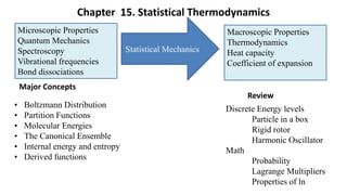
Chapter 15. Statistical Thermodynamics
Major Concepts
Review
Discrete Energy levels
Particle in a box
Rigid rotor
Harmonic Oscillator
Math
Probability
Lagrange Multipliers
Properties of ln
Microscopic Properties
Quantum Mechanics
Spectroscopy
Vibrational frequencies
Bond dissociations
Macroscopic Properties
Thermodynamics
Heat capacity
Coefficient of expansion
Statistical Mechanics
2. Statistical Thermodynamics
Statistical thermodynamics provides the link between the microscopic (i.e., molecular) properties of matter
and its macroscopic (i.e., bulk) properties. It provides a means of calculating thermodynamic properties
from the statistical relationship between temperature and energy.
Based on the concept that all macroscopic systems consist of a large number of states of differing energies,
and that the numbers of atoms or molecules that populate each of these states are a function of the
thermodynamic temperature of the system.
One of the first applications of this concept was the development of the kinetic theory of gases and the
resulting Maxwell-Boltzmann distribution of molecular velocities, which was first developed by Maxwell in
1860 on purely heuristic grounds and was based on the assumption that gas molecules in a system at thermal
equilibrium had a range of velocities and, hence, energies.
Boltzmann performed a detailed analysis of this distribution in the 1870’s and put it on a firm statistical
foundation. He eventually extended the concept of a statistical basis for all thermodynamic properties to all
macroscopic systems.
3.
2 2
3/2 3/2
v Mv
2 2
2 2
v 4 v 4 v
2 2
m
kT RT
m M
f e e
kT RT
Maxwell-Boltzmann Distribution:
5. Statistics and Entropy
Macroscopic state :- state of a system
is established by specifying its T, E ,S ...
Microscopic state :- state of a system is
established by specifying x, p, ε... of ind.
constituents
More than one microstate can lead to the
same macrostate.
Example: 2 particles with total E = 2
Can be achieved by microstates 1, 1 or
2, 0 or 0, 2
Configuration:- The equivalent ways to
achieve a state
W (weight):- The # of configurations
comprising a state
Probability of a state:- # configuration
in state / total # of configurations
(Assumes that the five molecules are distinguishable.)
6. Weight of a Configuration
0 1 2 3
0 1 2 3
0 1 2 3
!
! ! ! !
!
ln ln
! ! ! !
ln ! ln ! ! ! !
ln ! ln !
i
i
N
W
N N N N
N
W
N N N N
N N N N N
N N
Using Sterling’s Approximation:
ln N! ~ N ln N − N, which is valid for N » 1,
ln ln ln
i i
i
W N N N N
7. • Global maximum in f when df = 0 df
f
x
y
dx
f
y
x
dy
• Seek a maximum in f(x,y) subject to a constraint defined by g(x,y) = 0
• Since g(x,y) is constant dg = 0 and: dg
g
x
y
dx
g
y
x
dy 0
• This defines dx
g
y
g
x
dy and dy
g
x
g
y
dx
• Eliminating dx or dy from the equation for df: df
f
y
f
x
g
y
g
x
dy 0 or df
f
x
f
y
g
x
g
y
dx 0
• Defines undetermined multiplier
f
y
g
y
or
f
x
g
x
f
x
g
x
0 or
x
f g
0 f
y
g
y
0
y
f g
0
or
Same as getting unconstrained maximum of K f g
Undetermined Multipliers (Chemist’s Toolkit 15A.1)
8. Example of Undetermined Multipliers
A rectangular area is to be enclosed by a fence having a total length of 16
meters, where one side of the rectangle does not need fence because it is
adjacent to a river. What are the dimensions of the fence that will enclose
the largest possible area?
river
y
x x
Thus, the principal (area) function is: F(x,y) = xy (1)
and the constraint (16 meters) is: f(x,y) = 2x + y − 16 = 0 (2)
If F(x,y) were not constrained, i.e., if x and y were independent, then the derivative (slope) of F would be zero:
(3)
and
(4)
However, this provides only two equations to be solved for the variables x and y, whereas three equations must
be satisfied, viz., Eqs. (4) and the constraint equation f(x,y) = 0.
dF x y
F
x
dx
F
y
dy
( , )
0
0 and 0
F F
x y
9. Example of Undetermined Multipliers
The method of undetermined multipliers involves multiplying the constraint equation by another quantity, λ,
whose value can be chosen to make x and y appear to be independent. This results in a third variable being
introduced into the three-equation problem. Because f(x,y) = 0, maximizing the new function F’
F’(x,y) ≡ F(x,y) + λ f(x,y) (5)
is equivalent to the original problem, except that now there are three variables, x, y, and λ, to satisfy three
equations:
(6)
Thus Eq. 5 becomes
F’(x,y) = xy + λ (2x + y -16) (7)
Applying Eqs. (6),
yielding λ = −4, which results in x = 4 and y = 8. Hence, the maximum area possible is A = 32 m2.
' '
0 0 and ( , ) 0
F F
f x y
x y
'
2 0 2
F
y y
x
'
0
F
x x
y
2 16 2 2 16 0
x y
10. Find a maximum of f x,y
e
x2
y2
Subject to the constraint g x,y
x 4y 17 0
From slope formula df
f
x
y
dx
f
y
x
dy 0 df 2xe
x2
y2
dx 2ye
x2
y2
dy 0
Global maximum: x = y = 0 Need to find constrained maximum
• Find undetermined multiplier K(x,y) f (x,y) g(x, y) e
x2
y2
x 4y 17
• An unconstrained maximum in K must
K
x
2xe
x2
y2
0
K
y
2ye
x2
y2
4 0
2xf
y
2 f
• This implies 2x
y
2
4x y
• Original condition g = 0 g x,y
x 4 4x
17 0
• Constrained maximum : x = 1; y = 4
Example of Undetermined Multipliers
11. Most Probable Distribution
𝐸 =
𝑖
𝑁𝑖 ∈𝑖
𝑊 =
𝑁!
𝑁1! 𝑁2! 𝑁3! …
Configurations:
(permutations)
Total energy:
Maximum probability (and, hence, maximum entropy) occurs when each particle is in a different energy level.
But minimum energy occurs when all particles are in the lowest energy level. Thus, must find the maximum
probability that is possible, consistent with a given total energy, E, and a given total number of particles, N.
This is an example of a classic problem, in which one must determine the extrema (i.e., maxima and/or
minima) of a function, e.g. entropy, that are consistent with constraints that may be imposed because of other
functions, e.g., energy and number of particles. This problem is typically solved by using the so-called
LaGrange Method of Undetermined Multipliers.
Example: N = 20,000; E = 10,000; three energy levels 𝜖1 = 0, 𝜖2 = 1, 𝜖3 = 2.
Constant E requires that N2 + 2N3 = 10,000; constant N requires that N1 + N2 + N3 = 20,000
0 < N3 < 3333; W is maximum when N3 ~1300.
𝑁 =
𝑖
𝑁𝑖
Total number of particles:
12.
13. The most probable distribution is the one with greatest weight, W. Thus, must maximize lnW. Because there
are two constraints (constant E and constant N), must use two undetermined multipliers: g(xi) = 0 and h(xi) = 0
so K = (f + ag +bh)
• Use this to approach to find most probable population: K ln W a N Nj
j
b E Njj
j
(constant N) (constant E)
Want constrained maximum of lnW (equivalent to unconstrained maximum of K)
• Use Stirling's Approximation for lnW: K N ln N Nj ln Nj
j
a N Nj
j
b E Nj j
j
• Can solve for any single population Ni (all others 0):
N
Ni
0
Ni
Ni
1
Nj
Ni
0
K
Ni
lnNi Ni
1
Ni
a 1
b i
0
K
Ni
lnNi 1 a bi 0
ln Ni 1a
bi
Most Probable Distribution
14. N Nj
j
A e
b j
j
A N
e
bj
j
Ni
Nebi
e
bj
j
b
1
kbT
pi
Ni
N
e
i
kbT
e
j
kbT
j
A exp 1a
Ni Ae
bi
If , then
• A (a) can be eliminated
by introducing N:
Boltzmann Temperature (will prove later)
Boltzmann Distribution
Boltzmann Distribution
ln Ni 1a
bi
Τ
𝑁𝑖 𝑁𝑗 = e−𝛽 𝜀𝑖−𝜀𝑗 = e− Τ
𝜀𝑖−𝜀𝑗 𝑘𝑇
For relative populations:
Gives populations of states, not levels.
If more than one state at same energy, must account
for degeneracy of state, gi.
Τ
𝑁𝑖 𝑁𝑗 = Τ
𝑔𝑖 𝑔𝑗 e−𝛽 𝜀𝑖−𝜀𝑗
15. Most Probable Distribution
In summary, the populations in the configuration of greatest weight, subject to the constraints of fixed E and N,
depend on the energy of the state, according to the Boltzmann Distribution:
i
i
kT
i
kT
i
N e
N
e
The denominator of this expression is denoted by q and is called the partition function, a concept that is
absolutely central to the statistical interpretation of thermodynamic properties which is being developed here.
As can be seen in the above equation, because k is a constant (Boltzmann’s Constant), the thermodynamic
temperature, T, is the unique factor that determines the most probable populations of the states of a system that is
at thermal equilibrium.
16. Most Probable Distribution
If comparing the relative populations of only two states, εi and εj, for example,
i
i j
j
kT
i kT
j kT
N e
e
N
e
The Boltzmann distribution gives the relative populations of states, not energy levels. More than one
state might have the same energy, and the population of each state is given by the Boltzmann
distribution. If the relative populations of energy levels, rather than states, is to be determined, then
this energy degeneracy must be taken into account. For example, if the level of energy εi is gi-fold
degenerate (i.e., gi states have that energy), and the level of energy εj is gj-fold degenerate, then the
relative total populations of these two levels is given by:
i
i j
j
kT
i i i kT
j j
kT
j
N g e g
e
N g
g e
18. Example Partition Function: Uniform Ladder
Because the partition function for the uniform ladder
of energy levels is given by:
then the Boltzmann distribution for the populations in
this system is:
Fig. 15B.4 shows schematically how pi varies with
temperature. At very low T, where q ≈ 1, only the
lowest state is significantly populated. As T increases,
higher states become more highly populated. Thus,
the numerical value of the partition function gives an
indication of the range of populated states at a given T.
1 1
1
1 kT
q
e
e
b
(1 ) (1 )
i
i
i
i kT kT
i
N e
p e e e e
N q
b
b
b
19. Two-Level System
For a two-level system, the partition function and
corresponding population distribution are given
by:
and
1 1 kT
q e e
b
1
1
i
i i kT
i
kT
e e e
p
q e
e
b b
b
20. Two-Level System
In this case, because there are only two levels
and, hence, only two populations, p0 and p1,
and because ε0 = 0 and ε1 = 1, then
and
At T = 0 K, q = 1, indicating that only one state
is occupied. With increasing temperature, q
approaches 0.5, at which point both states are
equally populated. Thus, it can be generalized
that as T → ∞, all available states become
equally populated.
0
1 1
1
1 kT
p
e
e
b
1
1
1
kT
kT
e e
p
e
e
b
b
21. Generalizations Regarding the Partition Function
Conclusions regarding the partition function:
• Indicates the number of thermally accessible states in a system.
• As T → 0, the parameter β = 1/kT → ∞, and the number of populated states → 1, the lowest (ground)
state, i.e., , where g0 is the degeneracy of the lowest state.
• As T → ∞, each of the terms β = ε/kT in the partition function sum → 0, so each term = 1.
Thus, , since the number of available states is, in general, infinite.
• In summary, the molecular partition function q corresponds to the number of states that are thermally
accessible to a molecule at the temperature of the system.
0
0
lim
T
q g
i
e b
lim
T
q
22. Contributions to Partition Function
● Total energy of a molecule is the sum of the contributions from its different modes of motion
(translational, rotational, vibrational), plus its electronic energy:
● Thus, the partition function for the molecule consists of the product of the components from each
of the four individual types of energy:
g: degeneracy of the corresponding energy level
23. Translational Partition Function
● Translational energy levels are very closely spaced, thus, at normal
temperatures, large numbers of them are typically accessible.
● Assume that gas is confined in a three-dimensional volume.
● Quantum states can be modeled by a particle in a 3D box with side
lengths a, b, and c:
● The translational partition function for a single molecule is
2 2
2 2 2 2
2 2 2
( , , )
8 8 8
y
x z
x y z
n h
n h n h
E n n n
ma mb mc
2
2 2
2
2 2 2
2
2
2 2
2 2
2
2 2
8
1 1 1
8
8 8
1 1 1
y
x z
x y z
y
x z
x y z
n
n n
h
mkT a b c
T
n n n
n
h
n n
h h
mkT b
mkT mkT
a c
n n n
q e
e e e
24. ● For a system having macroscopic dimensions, the summations can be replaced by integrals:
● The above definite integrals evaluate to:
Thus,
● If the thermal de Broglie wavelength, Λ, is defined as , then
where Λ has units of length, and qT is dimensionless.
Translational Partition Function
2
2 2
2 2 2
2 2 2
8 8 8
0 0 0
y
x z
x y z
n
n n
h h h
T mkT mkT mkT
a b c
x y z
n n n
q e dn e dn e dn
3
T V
q
25. Example: Calculate the translational partition function for an O2 molecule in a 1 L vessel at 25oC.
Thus, under these conditions, an O2 molecule would have ~1029 quantum states thermally accessible to it.
The thermal wavelength of the O2 molecule (Λ = h/(2πmkT)1/2) is ~18 pm, which is ~eight orders of
magnitude smaller than the size of the containing vessel.
In order for the above equation for qT to be valid, the average separation of the particles must be much
greater than their thermal wavelength. Assuming that O2 molecules behave as a perfect gas at 298K and
1 bar, for example, the average separation between molecules is ~3 nm, which is ~168 times larger than
the thermal wavelength.
34
1/2 27 23 1/2
11
3 3
29
3 11 3 3
6.626 10 J×s
(2 ) (2 32 amu 1.67 10 kg/amu 1.38 10 J/K 298K)
1.78 10 m =17.8 pm
1 10 m
1.77 10
(1.78 10 ) m
T
h
mkT
V
q
Translational Partition Function
26. Translational Partition Function
As seen by its definition:
the three-dimensional translational partition function increases with the mass of the particle, as m3/2, and
with the volume, V, of the container.
For a given particle mass and container volume, qT also increases with temperature, as T3/2 because an
infinite number of states becomes accessible as the temperature increases:
qT → ∞ as T → ∞
3/2
3 3
2
T mkT
V
q V
h
27. ● The rotational energy of a rigid rotor is
where J is the rotational quantum number
(0, 1, 2,...) and I is the moment of inertia.
● The rotational partition function for a linear
molecule is thus
● where the rotational constant is given by: ෨
𝐵 = Τ
ℏ 4π𝑐𝐼
𝑞 𝑅
=
𝐽=0
∞
𝑔𝐽 𝑒−
𝐸𝑟𝑜𝑡
𝑘𝑇 =
𝐽=0
∞
2𝐽 + 1 𝑒
−
𝐽 𝐽+1 ℎ2
8𝜋2𝐼𝑘𝑇 =
𝐽=0
∞
2𝐽 + 1 𝑒−𝛽ℎ𝑐 ෨
𝐵𝐽 𝐽+1
Rotational Partition Function for Diatomic Molecules
B
28. ● For molecules with large moments of inertia or at sufficiently high temperature, the above sum
approximates to
● In general,
where σ is the symmetry number:
– σ = 1 for heteronuclear diatomic molecules
– σ = 2 for homonuclear diatomic molecules
• The temperature above which the approximation shown above for qR is valid is termed the
characteristic rotational temperature, θR, which is given by: .
• At sufficiently high temperatures (T » θR), the rotational partition function for linear molecules is:
Rotational Partition Function for Diatomic Molecules
/
R
hcB k
R
R
T
q
2
2
( 1) 2
( 1)
8
2
0
8 1
(2 1) (2 1)
J J h
R hcBJ J
IkT
IkT
q J e dJ J e dJ
h hcB
b
b
2
2
8 1
R IkT
q
h hcB
b
31. ● The rotational energy of linear polyatomic molecules is the same as for diatomics, with = 1 for
nonsymmetric linear molecules (HCN) and 2 for symmetrical molecules (CO2).
● General polyatomic molecules may have 3 different values of I (moments of inertia), and so have 3
different rotational temperatures.
– If symmetries exist, some of the moments of inertia may be equal.
Θ𝐴 =
ℎ2
8𝜋2𝐼𝐴𝑘
𝑞𝑟𝑜𝑡=
𝜋 ൗ
1
2
𝜎
𝑇3
Θ𝐴Θ𝐵Θ𝐶
ൗ
1
2
Rotational Partition Function for Polyatomic Molecules
• The symmetry number, , is the distinct
number of proper rotational operations, plus
the identity operator, i.e., the number is the
number of indistinguishable positions in
space that can be reached by rigid rotations.
32. Origin of Symmetry Numbers
Quantum mechanical in origin, viz., the Pauli principle forbids
occupation of certain states.
e.g. H2 occupies only even J-states if the nuclear spins are paired
(para-H2) and only odd J-states if the spins are parallel (ortho-H2).
Get about the same value as if each J term contributed only half its
normal value to the sum. Thus, must divide by =2.
Similar arguments exist for other symmetries, e.g. CO2:
33. Vibrational Partition Function
In the harmonic oscillator approximation, the vibrational
energy levels in a diatomic molecule form a uniform ladder
separated by ℏ𝜔 (= hc ǁ
𝜈).
ℏ𝜔 = ℎ𝜈
ℏ = ൗ
ℎ
2𝜋
𝜔 = 2𝜋𝜈
ǁ
𝜈 = Τ
𝜈
𝑐
Thus, using the partition function developed previously for a
uniform ladder (Example 15B.1):
At sufficiently high temperatures, such that T » θV,
1 1 1 1
1 1
1 1
V
V
hc
hc
kT T
q
e e
e e
b b
where θV is the characteristic vibrational temperature,
given by
V hc
k
V
V
kT T
q
hc
34. Vibrational Partition Function
In molecules having sufficiently strong bonds, e.g., C-H bonds (~1000 – 2000 cm-1), the vibrational
wavenumbers are typically large enough that . In such cases, the exponential term in the
denominator of qV approaches zero, resulting in qV values very close to 1, indicating that only the zero-
point energy level is significantly populated.
1
hc
b
By contrast, when molecular bonds are sufficiently weak that , qV may be approximated by
expanding the exponential (ex = 1 + x + …):
Thus, for weak bonds at sufficiently high temperatures:
1
hc
b
1 1 1
1 1 (1 ...)
1 1
V
hc
q
hc
e hc
kT
b
b
V kT
q
hc
36. Electronic Partition Function
● Except for hydrogen atoms, there are no simple formulas for
electronic energy levels from quantum mechanics.
● The partition function for electronic states is:
𝑞𝐸 =
𝑙𝑒𝑣𝑒𝑙𝑠
𝑔𝑖𝑒−𝛽𝜀𝑖 = 𝑔0𝑒−𝛽𝜀0 + 𝑔1𝑒−𝛽𝜀1 + ⋯
● Because the first excited electronic state is typically well
above the ground state, i.e., 𝜀1 − 𝜀0 ≫ kT, only the ground
state is populated.
● Exceptions are molecules with low lying electronic states,
such as NO, NO2 and O2.
Electronic, Vibrational and Rotational energy
levels for the hydrogen molecule.
38. Mean Molecular Energy
Because, as shown previously, the overwhelmingly most probable population in a system at temperature T
is given by the Boltzmann distribution, ( ), then 𝜀 =
1
𝑞
σ𝑖 ε𝑖𝑒−𝛽ℇ𝑖, where β = 1/kT.
1
i i
i
E
N
N N
For a system of non-interacting molecules, the mean energy of a molecule , relative to its ground state, is
just the total energy of the system, E, divided by the total number of molecules in the system, N:
/ /
i
i
N N e q
b
The latter relationship can be manipulated to express in terms only of q by recognizing that
Hence,
where the partial derivatives recognize that q may depend on variables (e.g., V) other than only T. Because
the above expression gives the mean energy of a molecule relative to its ground state, the complete
expression for is:
This result confirms the very important conclusion that the mean energy of a molecule can be calculated
knowing only the partition function (as a function of temperature).
( )
i
i
i
e
e
b
b
b
1 ( ) 1 1
i
i
i i V V
V
e q
e
q q q
b
b
b b b
1 ln
gs gs
V V
q q
q
b b
40. Translational Energy
Each of the three modes of motion (translational, rotational, and vibrational), as well as the potential energies
represented by the electronic state and electron spins, contributes to the overall mean energy of a system.
Translational Contribution:
As developed previously, for a three-dimensional container of volume V, the translational partition
function is given by
where Λ3 is essentially a constant multiplied by β3/2. Thus,
In one dimension,
3/2
3/2
3 3 3
2
2
T V V m V
q mkT
h h
b
3
3/2
3/2
3/2
3/2
1
d 1
d
d 1 3
d 2
2
3
T
T
V
T
V
T
q V
q V
C
V
V
k
C
b b
b
b b
b
b
b b
1
2
T
kT
41. Rotational Energy
As developed previously, the rotational partition function for a
linear molecule is given by:
2
2
( 1)
( 1)
8
(2 1) (2 1)
J J h
R hcBJ J
IkT
i i
q J e J e b
At sufficiently low temperatures, such that ,
the term by term sum for a non-symmetrical molecule gives
/
R
T hcB k
2 6
1 3 5 ...
R hcB hcB
q e e
b b
Taking the derivative of qR with respect to β gives
2 6
d
(6 30 ...)
d
R
hcB hcB
q
hcB e e
b b
b
Hence, 2 6
2 6
1 d (6 30 ...)
d 1 3 5 ...
R hcB hcB
R
R hcB hcB
q hcB e e
q e e
b b
b b
b
42. At high temperatures (T >> θR),
Thus,
1
R
R
T
q
hcB
b
1 d d 1
d d
d 1
d
1
R
R
R
q
hcB
q h
T
B
k
c
b
b b b
b
b b
b
Rotational Energy
43. Vibrational Energy
At high temperatures, T >> θV = ℎ𝑐 ǁ
𝜈/𝑘, so
𝜀𝑉 =
ℎ𝑐 ǁ
𝜈
e𝛽ℎ𝑐
𝜈 − 1
=
ℎ𝑐 ǁ
𝜈
1 + 𝛽ℎ𝑐 ǁ
𝜈 + ⋯ − 1
≈
1
𝛽
= 𝑘𝑇
As developed previously, the vibrational partition function
for the harmonic oscillator approximation is:
1
1
V
hc
q
e b
Because qV is independent of volume it can be differentiated
with respect to β:
2
d d 1
d d 1 (1 )
V hc
hc hc
q hc e
e e
b
b b
b b
and since the mean energy is given by
2
1 d
(1 )
d (1 ) 1
V hc hc
V hc
V hc hc
q hc e hc e
e
q e e
b b
b
b b
b
then
1
V
hc
hc
eb
However, because most values of θV are very high,
(> 1000K) this condition is seldom satisfied.
44. Equipartition of Energy
● Degrees of freedom receive equal amounts of energy,
each of ½ kT.
● In diatomic molecules at sufficiently high temperature:
– 3 translational degrees of freedom = 3/2 kT
– 2 rotational degrees of freedom = kT
– vibrational potential and kinetic energy = kT
● At sufficiently low temperatures, only the ground state
is significantly populated. This causes degrees of
freedom to freeze out and not contribute to the heat
capacity.
– This can be seen in the treatment of the vibrational
partition function, as well as in the two-level system
discussed previously.
– Note that the treatment of the rotational partition
function on the previous slides cannot predict the
freezing out of the rotational degrees of freedom,
because the energy levels were approximated as a
continuum using the integral.
45. Electronic & Electron Spin Energies
Because statistical energies are measured relative to the ground state, and only the ground
electronic state is usually occupied, then
and
𝜀S = Τ
2𝜇Bℬ e2𝛽𝜇Bℬ + 1
An electron spin in a magnetic field B can have two possible energy states (𝜀−1/2 = 0 and 𝜀+1/2 =
2𝜇Bℬ) and energy given by
where ms is the magnetic quantum number, and μB is the Bohr magneton (eћ/2me = 9.274 x 10⁻²⁴ J/T).
𝐸𝑚𝑠
= 2𝜇Bℬ𝑚𝑠
𝑞S
=
𝑚𝑠
𝑒−𝛽ℇ𝑚𝑠 = 1 + 𝑒−2𝛽𝜇Bℬ
0
E
1
E
q
Electronic Energies
Electron Spin Energies
The spin partition function is therefore
and the mean energy of the spin is
46. Internal Energy and the Partition Function
As described previously, the mean energy of a system of independent non-interacting molecules
is given by:
where β = 1/kT.
For a system containing N molecules, the total energy is thus , so the internal energy U(T) is:
N
ln
( ) (0) (0) (0)
V V
N q q
U T U N U U N
q
b b
If the system consists of interacting molecules (e.g., a non-ideal gas), then the canonical partition
function Q must be used:
1
V
q
q
b
ln
( ) (0)
V
Q
U T U
b
47. 𝐶𝑣 =
𝜕𝑈
𝜕𝑇 𝑉
𝜀𝑉 =
ℎ𝑐
𝜈
e𝛽ℎ𝑐
𝜈 − 1
=
𝑘𝜃𝑣
e
𝜃𝑣
𝑇 − 1
Recall that the constant-volume heat capacity is:
As shown previously, the mean vibrational energy of a collection of harmonic oscillators is given by
where is the characteristic vibrational temperature. Thus, the vibrational contribution to
the molar heat capacity at constant volume is
/
V
hc k
2 /
, 2
/ /
d d 1
d d 1 1
V
V
V
V V T
V V
A
v m T T
N e
C R R
T T T
e e
or, expressed as a function of temperature:
2
2 /2
, /
( ), where ( )
1
V
V
V T
V
v m T
e
C Rf T Rf T
T e
Heat Capacity and the Partition Function
48. 𝐶𝑣 = −𝑘𝛽2
𝜕𝑈
𝜕𝛽 𝑉
= −N𝑘𝛽2
𝜕 𝜀
𝜕𝛽 𝑉
= 𝑁𝑘𝛽2
𝜕2
𝑙𝑛𝑞
𝜕𝛽2
𝑉
If the derivative with respect to T is converted into a derivative with respect to β, then Cv can be
expressed as
If T >> θM, where θM is the characteristic temperature of
each mode ( ), then the
equipartition theorem can be applied. In this case, each
of the three translational modes contributes ½ R. If the
rotational modes are represented by νR*, then νR* = 2 for
linear molecules and 3 for non-linear molecules, so the
total rotational contribution is ½ νR*R. If the temperature
is sufficiently high for νV* vibrational modes to be active,
then the vibrational contribution is νV*R. Thus, the total
molar heat capacity is:
In most cases, νV* = 0.
/ and /
R V
hcB k hc k
CV,m = ½ (3 + R* + 2V*)R
Heat Capacity and the Partition Function
49. Entropy and the Partition Function
Boltzmann equation: S = k lnW
where S is the statistical entropy, and W is the weight of the most probable configuration of the system.
The Boltzmann Equation is one of the most important relationships in statistical thermodynamics, and
the statistical entropy is identical to the thermodynamic entropy, behaving exactly the same in all
respects.
• As the temperature decreases, for example, S decreases because fewer configurations are consistent
with the constant total energy of the system.
• As T → 0, W → 1, so ln W = 0, since only one configuration (viz., the one in which every molecule
is in the lowest level) is consistent with E = 0.
• As S → 0, T → 0, which is consistent with the Third Law of thermodynamics, i.e., that the entropies
of all perfect crystals approach zero as T → 0.
50. Entropy and the Partition Function
Relationship of Boltzmann Equation to the partition function
• For a system of non-interacting and distinguishable molecules,
• For a system of non-interacting and indistinguishable molecules
(e.g., a gas of identical molecules),
• For a system of interacting molecules, use the canonical partition
function,
( ) (0)
( ) ln
U T U
S T Nk q
T
( ) (0)
( ) ln
U T U q
S T Nk
T N
( ) (0)
( ) ln
U T U
S T Nk Q
T
51. Entropy and the Partition Function
As shown previously, the total energy of a molecule can be closely approximated by the sum of
the independent contributions from translational (T), rotational (R), vibrational (V), and electronic
(E) energies. The total entropy can be similarly treated as a sum of individual contributions.
• For a system of distinguishable, non-interacting molecules, each contribution has the form of
that for S(T) above:
(for M = R, V, or E)
• For M = T, the molecules are indistinguishable, so
( ) (0)]
( ) ln
M
M
U T U
S T Nk q
T
( ) (0)]
( ) ln
T T
U T U q
S T Nk
T N
52. Translational Entropy: The Sackur-Tetrode Equation
For a system consisting of a perfect monatomic gas, only translation contributes to the total energy
and molar entropy, which is described by the Sackur-Tetrode Equation:
where Λ is the thermal wavelength (h/(2πmkT)1/2 described previously, Vm is the molar volume, NA is
Avogadro’s Number, and R/NA = k.
Since for a perfect gas Vm = RT/p, then Sm can be calculated from
Re-writing the Sackur-Tetrode Equation in the form:
shows that when a perfect monatomic gas expands isothermally from Vi to Vf, ΔS is given by:
which is identical to the expression determined from the thermodynamic definition of entropy.
3/2
5/2 5/2 5/2
3 3 3
2
ln ln ln
m m m
m
A A
V e mkT V e V e
S R R k
N h N
5/2 5/2
3 3
ln ln
m
A
RTe kTe
S R R
p N p
5/2 5/2
3 3
ln ln , where
A A
Ve e
S nR nR aV a
nN nN
ln ln ln
f
f i
i
V
S nR aV nR aV nR
V
53. Entropy: Rotational Contribution
At sufficiently high temperatures, where ,
which is usually the case, then , and
the equipartition theorem predicts the rotational contribution
to the molar entropy to be RT. Therefore,
Hence, this relationship indicates that
• The rotational contribution to the entropy increases with
increasing T because more rotational states become
accessible.
• The rotational contribution will be large when the
rotational constant is small because then the rotational
levels are more closely spaced.
( / )
R
T hcB k
/ /
R R
q kT hcB T
(0)
ln 1 ln 1 ln
R R
m
m R
U U kT T
S R q R R
T hcB
B
54. Entropy: Vibrational Contribution
The vibrational contribution to the molar entropy, SV
m , can be
obtained by combining qV (= 1/(1 – e‒βε) with ,
the mean vibrational energy:
where the final equality occurs because .
• Both terms in the right-hand equality approach 0 as T → 0,
so S = 0 at T = 0.
• S increases as T increases because more vibrational states
become thermally accessible.
• At a given T, S is larger for higher M.W. molecules than for
lower M.W. because their energy levels are more closely
spaced, and thus more are thermally accessible.
/ 1
V
eb
(0) 1
ln ln
1 1
ln 1 ln 1
1 1
V V
m m A
m
hc
hc
U U N k
S R q R
T e e
hc
R e R e
e e
b b
b b
b b
b
b b
hc
55. Derived Functions: Enthalpy and Gibbs Energy
𝑆 𝑇 =
𝑈 𝑇 − U 0
𝑇
+ 𝑘𝑙𝑛𝑄
𝑈 𝑇 = U 0 −
𝜕𝑙𝑛𝑄
𝜕𝛽 𝑉
The partition function also can be used to calculate the pressure, enthalpy, and Gibbs Energy:
Can use various thermodynamic relationships to calculate other quantities. In all of the equations below,
the canonical partition function Q is related to the molecular partition function q by Q = qN for
distinguishable molecules, and Q = qN/N! for indistinguishable molecules (e.g., as in a gas).
As shown previously, the internal energy and entropy are related to the partition function as follows:
𝐻 = 𝑈 + 𝑃𝑉 𝐻 𝑇 = H 0 −
𝜕𝑙𝑛𝑄
𝜕𝛽 𝑉
+𝑘𝑇𝑉
𝜕𝑙𝑛𝑄
𝜕𝑉 𝑇
𝐺 = 𝐻 − 𝑇𝑆 = 𝐴 + 𝑃𝑉 𝐺 𝑇 = G 0 − 𝑘𝑇𝑙𝑛𝑄+𝑘𝑇𝑉
𝜕𝑙𝑛𝑄
𝜕𝑉 𝑇
𝐺 𝑇 = G 0 − 𝑛𝑅𝑇𝑙𝑛
𝑞
𝑁
(From 𝑄 = Τ
𝑞𝑁 𝑁! 𝑎𝑛𝑑 𝑙𝑛𝑄 = 𝑁𝑙𝑛𝑞 − 𝑙𝑛𝑁! 𝑎𝑛𝑑 𝑙𝑛𝑁! = 𝑁𝑙𝑛𝑁 − 𝑁)
𝐺 𝑇 = G 0 − 𝑛𝑅𝑇𝑙𝑛
𝑞𝑚
𝑁𝐴
56.
57.
58. Equilibrium Constants
As shown previously, the equilibrium constant K of a reaction is related to the standard Gibbs
energy of reaction, ΔrGo, (p = 1 bar) by:
ΔrGo = ‒RTlnK
From statistical thermodynamics, the Gibbs energy is related to the molar partition function by:
qm = q/n and
In order to calculate a value for K, these equations must be combined. To develop an expression
for K, the standard molar Gibbs energy, Go/n, must be determined for each reactant and product in
the reaction. For the gas-phase reaction,
it can be shown that the equilibrium constant is given by:
𝐺 𝑇 = G 0 − 𝑘𝑇𝑙𝑛𝑄+𝑘𝑇𝑉
𝜕𝑙𝑛𝑄
𝜕𝑉 𝑇
o
o o
, , /
o o
, ,
( / ) ( / )
( / ) ( / )
r
c d
C m A D m A E RT
a b
A m A B m A
q N q N
K e
q N q N
aA bB cC dD
59. Equilibrium Constants
where ΔrEo is the difference in molar energies of the ground
states of the products and reactants and is calculated from the
bond dissociation energies of the various reaction species, i.e.,
Do(products) – Do(reactants).
Using the symbolism of (signed) stoichiometric numbers that
was introduced previously, K is given by:
o
o
, /
J
r
J m E RT
J A
q
K e
N
61. Contributions to equilibrium constants
For the reaction R → P, assume that R has only a single accessible level, so that qR = 1, and that P
has a large number of closely spaced levels, so that qP = kt/ε. The equilibrium constant is:
• It can be seen that when ΔrEo is very large, the exponential term dominates, and K << 1,
indicating that very little P is present at equilibrium.
• When ΔrEo is small, but positive, K can exceed 1 because the factor kT/ε may be large enough
to offset the low value of the exponential term. The size of K then results from the large
amount of P at equilibrium resulting from its high density of states.
• At low temperatures, K << 1, and R predominates at equilibrium.
• At high temperatures, the exponential function approaches 1, and P becomes dominant.
• For this endothermic reaction, a temperature increase favors P because its states become
increasingly accessible as the temperature increases.
o /
r E RT
kT
K e