Download as PDF, PPTX


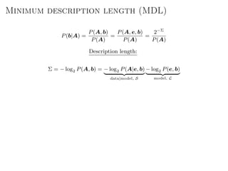


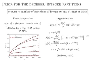


![Inference algorithm: Metropolis-Hastings
Move proposal, bi = r → bi = s
Accept with probability
a = min 1,
P(b |A)P(b → b )
P(b|A)P(b → b)
.
Move proposal of node i requires O(ki) operations. A whole MCMC sweep
can be performed in O(E) time, independent of the number of
groups, B.
In contrast to:
1. EM + BP with Bernoulli SBM: O(EB2
) (Semiparametric) [Decelle et al, 2011]
2. Variational Bayes with (overlapping) Bernoulli SBM: O(EB) (Semiparametric) [Gopalan
and Blei, 2011]
3. Bernoulli SBM with noninformative priors: O(EB2
) (Greedy) [Cˆome and Latouche, 2015]
4. Poisson SBM with noninformative priors: O(EB2
) (heat bath) [Newman and Reinert, 2016]](https://image.slidesharecdn.com/presentation-170913155059/85/Statistical-inference-of-network-structure-103-320.jpg)
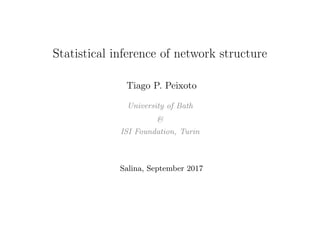
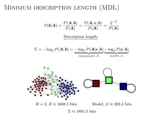
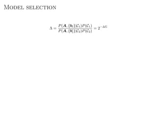
![Efficient inference: other improvements
Smart move proposals
Choose a random vertex i
(happens to belong to group r).
Move it to a random group
s ∈ [1, B], chosen with a
probability p(r → s|t) proportional
to ets + , where t is the group
membership of a randomly chosen
neighbour of i.
i
bi = r
j
bj = t
etr
ets
etur
t
s
u
Fast mixing times.
Agglomerative initialization
Start with B = N.
Progressively merge groups.
Avoids metastable states.](https://image.slidesharecdn.com/presentation-170913155059/85/Statistical-inference-of-network-structure-104-320.jpg)


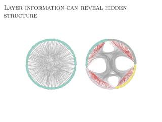


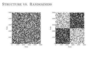
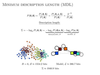
![Better approach: Metadata as data
Main idea: Treat metadata as data, not “ground truth”.
Generalized annotations
Aij → Data layer
Tij → Annotation layer
D
ata,
A
M
etad
ata,
T
Joint model for data and
metadata (the layered SBM [1]).
Arbitrary types of annotation.
Both data and metadata are
clustered into groups.
Fully nonparametric.](https://image.slidesharecdn.com/presentation-170913155059/85/Statistical-inference-of-network-structure-153-320.jpg)


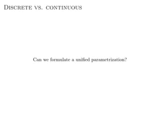
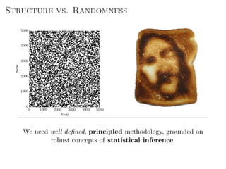
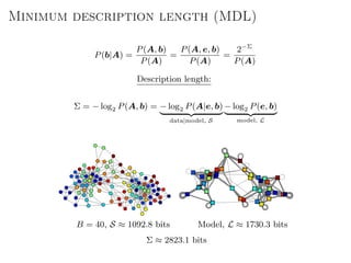
![The Graphon
P(G|{xi}) =
i>j
p
Aij
ij (1 − pij)1−Aij
pij = ω(xi, xj)
xi ∈ [0, 1]
Properties:
Mostly a theoretical tool.
Cannot be directly inferred (without massively overfitting).
Needs to be parametrized to be practical.](https://image.slidesharecdn.com/presentation-170913155059/85/Statistical-inference-of-network-structure-179-320.jpg)


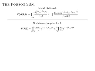
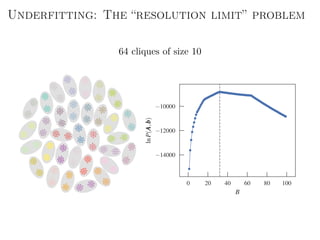
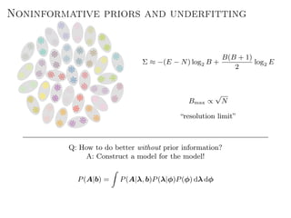
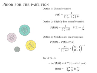
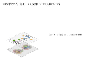
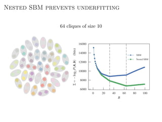
The document discusses Bayesian statistical inference for characterizing the structure of large networks. It introduces stochastic blockmodels as a generative model for network structure and describes performing Bayesian inference on these models. This involves defining a likelihood function based on a stochastic blockmodel, placing prior distributions on the model parameters, and computing the posterior distribution over partitions using Bayes' rule. Statistical inference provides a principled means of inferring community structure without overfitting and enables model selection among different partitions. Examples analyzing real networks demonstrate its ability to uncover meaningful structure.