Several researches have been conducted to study the impact of different macro-economic variables and their influence on government expenditure. By using different statistical tools researchers have examined that how money supply and exchange rate influence the government expenditure. Few other studies also conducted work on the quarterly time series data to examine the long run equilibrium association between the macroeconomic variables.
This paper studies the causal relationship between inflation and economic growth in Qatar for the period of 1980 to 2016. A time series analysis of unit roots tests, Johansen cointegration method and Granger causality tests were applied on data. The variables were found to be cointegrated, hence a long run-relationship between them exists. Granger causality test found causality runs from inflation to economic growth.
This paper studies the causal relationship between inflation and economic growth in Qatar for the period of 1980 to 2016. A time series analysis of unit roots tests, Johansen cointegration method and Granger causality tests were applied on data. The variables were found to be cointegrated, hence a long run-relationship between them exists. Granger causality test found causality runs from inflation to economic growth.
This paper examine the impact of macroeconomic factors on firm level equity premium. Following
the concept of macro-based risk factor model, we consider macroeconomic variable set of equity premium
determinant. The macroeconomic variables include interest rate, money supply, industrial production, inflation
and foreign direct investment. The macroeconomic variables are not in control of the firm's management. These
are the external factors which affect the company as well as the overall market returns. The Macro-based
Multifactor Model is estimated for the whole sample. It is found that the market premium and the selected five
macroeconomic factors significantly affect the firm level equity premium of non-financial firms. Increase in
market premium, money supply, foreign direct investment and industrial production positively affect the firm
level equity premium while increase in interest rate and inflation negatively affects the firm level equity
premium. These findings are beneficial for the common shareholders, institutional investors and policy makers
to find more specific insight about the relationship between macroeconomic variables and equity premium of
non-financial sectors.
The objective of this study is to identify the determinants of inflation in West Africa, mainly in the WAEMU zone, in order to contribute to improving the conduct of monetary policy. The equation of the exchange of the Quantitative Theory of the Currency and the generalized method of moments (MMG) in dynamic panel is used. Annual data concerning six countries in West Africa and range from 1991 to 2015. The results of the estimation show that in addition to the economic growth rate and the money supply, the devaluation has a significant effect on inflation. As we can see, inflation is not systematically a monetary phenomenon in West Africa. The authorities must therefore seek to determine the optimal threshold for the rate of increase of the money supply.
The Effect of Money Supply on InflationHuongHoang70
A study of how money supply affects inflation. The results show that a higher quantity of money supply is not always a cause of inflation.
Multiple linear regression and the GLS method were applied with the use of #Stata software for this research.
However, some additional modifications are needed to improve the model's goodness of fit and more endogenous factors should be added.
Future study might be: Would stimulus packages cause stagflation?
Using a series of econometric techniques, the study analysed interaction between monetary policy and private sector credit in Ghana. This study made use of monthly dataset spanning January 1999 to December 2019 of credit to the private sector (PSC) and broad money supply (M2). The results reveal that there exists cointegration, a long run stationary relation between monetary policy and private sector credit. This implies, increases in credit should prompt long-term increases in monetary policy. It is not surprising that growth in the private sector might have a stronger effect on monetary policy. The Error Correction Test is statistically significant and that all the variables demonstrate similar adjustment speeds. This implies that in the short run, both money supply and credit are somewhat equally responsive to their last period’s equilibrium error. There is unidirectional causation from private sector credit to monetary policy. It can be said that, there is an interaction between money supply and private sector credit. Thus, credit to private sector holds great potential in promoting economic growth. It can be recommended to the government to increase the credit flow to the private sector because of its strategic importance in creating and generating growth of the economy.
Savings-Growth-Inflation nexus in Asia: Panel Data Approachiosrjce
The present study examines the savings-growth-inflation nexus in Asia through panel data approach
for the period 1981 to 2011. The inter-relationship between saving and economic growth is found to be
significant and unidirectional running from saving to economic growth. Economic growth negatively and
significantly affects inflation but inflation positively and significantly affects saving which supports Deaton’s
hypothesis. The variables such as saving, trade openness and population growth are found to be significant
determinants economic growth. Except GDP, variables such as real interest rate, inflation, dependency ratio
and literacy rate are found to be significant determinants of saving rate. Similarly, variables such as money
supply, growth rate and real interest rate are found to be the major determinants of inflation. No country
specific effects has been found for explaining growth rate of per capita real GDP but in case of saving rate and
inflation rate, many countries exhibit individual effects which are modeled as fixed effects in the panel data
framework. As contrary to the time invariant country fixed effects, there is no consistent country invariant year
fixed effect on real GDP per capita growth rate and saving rate, while there is highly significant negative effect
on inflation. As saving affects GDP per capita growth positively and significantly, policies should be framed in
such a way that encourage savings in Asian economies which in turn may lead sustained higher GDP per capita
growth.
This study examines whether economic stability in Indonesia capable predicted by the model Mundell-Fleming. Prediction proxy stability of the interaction of fiscal and monetary policy. During Indonesia's economic stability is largely determined by the strength of economic fundamentals, while economic fundamentals are strongly influenced by fiscal and monetary policies. Therefore flemming Mundell predicts how strong the economic stability in Indonesia ?, the statement in the analysis by using a long-term predictions are Vector Autoregression. Research findings indicate patterns of interaction predictions variety of fiscal and monetary policy, both short term, medium term and long term. It turned out that fiscal policies are derived from taxes are more effective than government spending to control economic growth, investment and inflation, but government spending is more effective to control the exchange rate. The monetary policy of interest rates more effectively control the exchange rate and inflation, while the money supply is more effective in controlling the growth of economy and investment.
Empirical Analysis of Fiscal Dominance and the Conduct of Monetary Policy in ...AJHSSR Journal
The study empirically investigates fiscal dominance and the conduct of monetary policy in
Nigeria, using quarterly data from 1986Q1 to 2016Q4. It adopts the vector error correction mechanism (VECM)
and cointegration technique to analyze the data and make inference. The findings reveal that there is no
evidence of fiscal dominance in Nigeria. The empirical results show that budget deficit, domestic debt and
money supply have no significant influence on the average price level. However, budget deficit and domestic
debt are shown to have significant influence on money supply, but only in the short-run. The policy implication
is that the government should enforce fiscal discipline through the appropriate institution and the Central Bank
should be given autonomy to perform the primary function of long-term price stability, among other functions.
Government budget control under the period of inflation: Evidence from Madaga...iosrjce
Madagascar is rich in resource undermine, maritime and natural but have been experiencing
Inflation now for more than four decades. Many studies and papers talk about the relationship between Inflation
and Budget Deficit. This paper seeks to test the hypothesis that budget control explicated by the budget deficit
cause inflation in Madagascar with some variable economically affect the inflation such as Gross Domestic
Product, exchange rate, Money supply, budget deficits and political crises that is during a thirty-three years
period: from 1981to 2014. The methodology employed for estimating long-run relationship is Augmented Ducky
Fuller test for a stationary data then cointegration analysis, with undertaking Granger causality tests. The
findings of the study are Malagasy Budget control is not inflationary and the inflation didn’t explain the budget
control. But the variable that cause the inflation in Madagascar are the Political Crises and Money Supply
DARSHANA ARADHYE
Mobile: +91-9099910969 / 0869078757 ~ E-Mail: darshanaaradhye@yahoo.com
Dear Sir/ Madam,
Please find attached my Resume for the position of equivalent job . I'm particularly interested in this position, which relates strongly to my over 11 years of experience in teaching ,administration ,curriculum framing, staff management
Currently working with Global India International as academic co ordinator for primary
Worked also as Head mistress with Pinnacle public school, Gandhinagar., Gujarat , I believe I meet all the essential criteria of the position. Few of my highlights of experience and demonstrated talent I would bring to your organisation include:
(a) Curriculum framing and setting up systems like lesson plan, time table, H.W. time table
(b) Review of team members
(c) Submission of MIS documents
(d) Guiding teachers for activity based teaching
(e) Organizing various events like –Sport’s day, Grandparents ‘s day, father ‘s day out ,convocation,CCE activities ,Annual functions and many other activities carried out in the school
(f) Leading team of 46 teacher, supervised 400 hundred children and support staff
I am now looking to take up roles as a vice principal /equivalent in a well known organisation. Of particular interest to me would be in this position.
I appreciate your taking the time to review my credentials and experience. Looking forward to a positive response.
Thanking you.
Sincerely,
Darshana Aradhye
Enclosure: Resume
DARSHANA ARADHYE
Mobile: +91-9099910969 / 0869078757 ~ E-Mail: darshanaaradhye@yahoo.com
PAUG 03/05/2016 : Rechercher et analyser les fuites mémoires dans une applica...Ludovic ROLAND
Dans cette présentation au format cours, l'objectif est de sensibiliser les développeurs au fait que même si la mémoire en Java ça ne se gère pas comment en C, il convient tout de même de faire attention car les fuites mémoires existent et sont souvent à l'origine de l'exception OutOfMemoryError.
Nous verrons comment générer un fichier hprof afin d'analyser l'empreinte mémoire d'une application dans l'outil dédié MAT (Eclipse Memory Analyzer) et mettre en avant la présence ou non de fuite mémoire.
Une brève introduction à la bibliothèque leakcanary sera également faite. Il s'agit d'une bibliothèque permettant de détecter des fuites mémoire lorsqu’un utilisateur navigue au sein d’une application (très utile pour détecter des fuites mémoires pendant les phases de développement et de recette).
aplikasi gallery pengetahuan ini diciptakan untuk menambah wawasan anak-anak dalam mengenal lingkungannya dan peran orang tua juga sangat penting dalam pembelajaran ini. Aplikasi gallery pengetahuan ini untuk anak-anak yang dikemas dalam media gambar yang berisi tentang pengenalan benda, buah, bunga, hewan, sayur, dan warna. aplikasi ini dapat membantu orang tua dalam mendidik anaknya dalam belajar mengenali gambar dan membaca
Desenvolvendo aplicações Cross-Platform com XamarinJúnior Porfirio
Desenvolver em múltiplas plataformas tem sido um desafio para os desenvolvedores e corporações. Com Xamarin esse desafio se torna mais simples. Objetivo dessa palestra é realizar uma introdução ao tema e demonstrar através de demos o poder dessa tecnologia para as plataformas IOS, Windows Phone e Android.
This study is about the impact of selected macroeconomic variables on economic growth of Bangladesh. Economic growth of Bangladesh is measured in terms of annual nominal GDP growth rate. Least squared regression model has been employed considering exchange rate, export, import and inflation rate as independent variables and gross domestic product as the dependent variable in this study. The results reveal that export and import have significant positive impact on GDP growth rate. The other variables (exchange rate and inflation) are not significant, indicating that there exists no significant relationship among the variables. The findings will help the policy makers to make policies concerning the country’s economic growth to remain robust in the near future.
Government Expenditure and Economic Growth Nexus: Empirical Evidence from Nig...iosrjce
This study has examined the impact of public expenditure on economic growth in Nigeria using time
series data for the period 1970-2012. Secondary data were sourced from the CBN, NBS, journals, text books
etc. The adopted model was fitted with three variables: real GDP, capital and recurrent expenditure. The tools
of analysis were the ADF unit root test and ordinary least square multiple regression accompanied by pairwise
Granger causality test. The major objective of this study is to analyse the impact as well as direction of
causality between the fiscal variables and economic growth. All the variables included in the model are
stationary at level. Empirical findings from the study show that there is positive and insignificant relationship
between capital expenditure and economic growth while recurrent expenditure had a significant positive impact
on economic growth. Also, Granger causality test demonstrates a unidirectional causality running from the
fiscal variables to economic growth in validation of the Keynesian theory. Consequently, the study
recommended more allocation of resources for recurrent purposes as well; government should establish the
body that will monitor contract awarding process of capital projects closely, to guard against over estimation of
project cost and stealing of public funds.
An Analysis of the Relationship between Fiscal Deficits and Selected Macroeco...IOSR Journals
This study investigates the relationship that exists between the Government Deficit Spending and selected macroeconomic variables such as Gross Domestic Product (GDP), Exchange Rate, Inflation, Money Supply and Lending Interest Rate. The period covered is 1970 (when the civil war ended) and 2011. Ordinary Least Squares (OLS) technique was adopted to analyze the relationships. The study concludes that Government Deficit Spending (GDS) has positive significant relationship with GDP. Government Deficit Spending also has positive significant relationship with Exchange Rate, Inflation, and Money Supply. Government Deficit has negative significant relationship with Lending Interest Rate and most likely crowd-out the private sector by raising the cost of funds. Deficit spending has been known to have adverse effects on the economy and government is advised to curtail excessive deficit spending. It is recommended that further research is done to establish other variables that are affected by government deficit spending.
The main focus of this study is to investigate the impact of expansion in economic growth on
government expenditure in Nigeria covering the periods 1970 to 2012. Gross Domestic Product (GDP) was
used as a proxy for economic growth, and the GDP time series was decomposed using the partial sum approach
in order to achieve asymmetry in the variable. The asymmetric ARDL estimation technique was appropriately
employed in this study. The findings of this study revealed that expansion in economic growth has significant
impact on government expenditure in Nigeria. The study further provided evidence of long-run causality from
boom/expansion in economic growth to government expenditure in Nigeria but could not support any evidence
of short-run causality. The researcher recommended among others, that Governments in Nigeria should give
more impetus to policies that will guarantee sustainable economic growth.
Effect of Government Policies on Price Stability in Nigeriaijtsrd
This study examined the effect of monetary and fiscal policies on price stability in Nigeria using a data rich framework spanning from 1986 2020. The main problem with the macro economic policies that prompted this study was the fact that despite the series of the CBN Monetary Policy Committee decisions and government tax and expenditure implementation there is apparently no useful effect on inflation price . The study employed Auto regression Distributed Lag ARDL Bound Test for Co integration of data analysis depending upon the time series properties of the data that confer mixed order of integration in addition to the conduct of the unit root test and Error Correction Model ECM estimation. The ADF test revealed that LNCPI, EXR, GSDMD, GEXP, GTX and M2 were stationary at 1 1 while RIR, MPR and BOP at 1 0 . Pesaran, Shin and Smith 2001 established that the ARDL bounds technique allows a mixture of 1 1 and 1 0 variables as regressors. Hence, we proceed to perform the ARDL bounds test for integration. The results of the ARDL bounds revealed that the null hypotheses were all rejected implying that a long run effect exists among monetary and fiscal policies variables and CPI in a multivariate framework. ECM coefficient of 0.2942 conforms with expectation. Durbin Watson statistic 0f 1 9925 revealed that the model seems not to have any case of autocorrelation. The result of our analysis shows that fiscal policy rather than monetary policy exerts a more potent effect on price stability in Nigeria. The study recommends that both monetary and fiscal policies should be complementary in order to be effective in taming inflation in Nigeria. Onehi, Damian Haruna | Ibenta, Steve Nkem | Adigwe, Patrick, K. | Emejulu, Ikenna Justin "Effect of Government Policies on Price Stability in Nigeria" Published in International Journal of Trend in Scientific Research and Development (ijtsrd), ISSN: 2456-6470, Volume-7 | Issue-1 , February 2023, URL: https://www.ijtsrd.com/papers/ijtsrd52766.pdf Paper URL: https://www.ijtsrd.com/management/accounting-and-finance/52766/effect-of-government-policies-on-price-stability-in-nigeria/onehi-damian-haruna
Inflation is a continual increase in general price level of goods and services in an economy over a period of time. It is caused by many factors, important among them are excess of demand of goods and services over supply, macroeconomic performance, money supply, economic policies implications, environmental factors etc. A number of researchers in the past made attempts to identify determinants of inflation and to investigate the impact of identified variables on inflation in European and also in some Asian economies. But, in context of India, not many studies can be traced in the literature. The purpose of this paper is to shed some light on the impact of selected variables on inflation in India. The paper considers CPI (Consumer Price Index) inflation as dependent variable and a set of independent macroeconomic variables, which includes Gross Domestic Product, Money Supply, Deposit Rate, Prime Lending Rate, Exchange Rate, Trade Volume (Value of Imports and Exports) and Crude Oil Prices. The empirical analysis covers the quarterly data series for ten financial years from 2002Q1 to 2012Q1. The collected data is analyzed using ADF Unit root test, Granger Causality test, and the Ordinary Least Square (OLS) technique.
USDA Loans in California: A Comprehensive Overview.pptxmarketing367770
USDA Loans in California: A Comprehensive Overview
If you're dreaming of owning a home in California's rural or suburban areas, a USDA loan might be the perfect solution. The U.S. Department of Agriculture (USDA) offers these loans to help low-to-moderate-income individuals and families achieve homeownership.
Key Features of USDA Loans:
Zero Down Payment: USDA loans require no down payment, making homeownership more accessible.
Competitive Interest Rates: These loans often come with lower interest rates compared to conventional loans.
Flexible Credit Requirements: USDA loans have more lenient credit score requirements, helping those with less-than-perfect credit.
Guaranteed Loan Program: The USDA guarantees a portion of the loan, reducing risk for lenders and expanding borrowing options.
Eligibility Criteria:
Location: The property must be located in a USDA-designated rural or suburban area. Many areas in California qualify.
Income Limits: Applicants must meet income guidelines, which vary by region and household size.
Primary Residence: The home must be used as the borrower's primary residence.
Application Process:
Find a USDA-Approved Lender: Not all lenders offer USDA loans, so it's essential to choose one approved by the USDA.
Pre-Qualification: Determine your eligibility and the amount you can borrow.
Property Search: Look for properties in eligible rural or suburban areas.
Loan Application: Submit your application, including financial and personal information.
Processing and Approval: The lender and USDA will review your application. If approved, you can proceed to closing.
USDA loans are an excellent option for those looking to buy a home in California's rural and suburban areas. With no down payment and flexible requirements, these loans make homeownership more attainable for many families. Explore your eligibility today and take the first step toward owning your dream home.
How to get verified on Coinbase Account?_.docxBuy bitget
t's important to note that buying verified Coinbase accounts is not recommended and may violate Coinbase's terms of service. Instead of searching to "buy verified Coinbase accounts," follow the proper steps to verify your own account to ensure compliance and security.
The Evolution of Non-Banking Financial Companies (NBFCs) in India: Challenges...beulahfernandes8
Role in Financial System
NBFCs are critical in bridging the financial inclusion gap.
They provide specialized financial services that cater to segments often neglected by traditional banks.
Economic Impact
NBFCs contribute significantly to India's GDP.
They support sectors like micro, small, and medium enterprises (MSMEs), housing finance, and personal loans.
how to sell pi coins in all Africa Countries.DOT TECH
Yes. You can sell your pi network for other cryptocurrencies like Bitcoin, usdt , Ethereum and other currencies And this is done easily with the help from a pi merchant.
What is a pi merchant ?
Since pi is not launched yet in any exchange. The only way you can sell right now is through merchants.
A verified Pi merchant is someone who buys pi network coins from miners and resell them to investors looking forward to hold massive quantities of pi coins before mainnet launch in 2026.
I will leave the telegram contact of my personal pi merchant to trade with.
@Pi_vendor_247
where can I find a legit pi merchant onlineDOT TECH
Yes. This is very easy what you need is a recommendation from someone who has successfully traded pi coins before with a merchant.
Who is a pi merchant?
A pi merchant is someone who buys pi network coins and resell them to Investors looking forward to hold thousands of pi coins before the open mainnet.
I will leave the telegram contact of my personal pi merchant to trade with
@Pi_vendor_247
how can i use my minded pi coins I need some funds.DOT TECH
If you are interested in selling your pi coins, i have a verified pi merchant, who buys pi coins and resell them to exchanges looking forward to hold till mainnet launch.
Because the core team has announced that pi network will not be doing any pre-sale. The only way exchanges like huobi, bitmart and hotbit can get pi is by buying from miners.
Now a merchant stands in between these exchanges and the miners. As a link to make transactions smooth. Because right now in the enclosed mainnet you can't sell pi coins your self. You need the help of a merchant,
i will leave the telegram contact of my personal pi merchant below. 👇 I and my friends has traded more than 3000pi coins with him successfully.
@Pi_vendor_247
Falcon stands out as a top-tier P2P Invoice Discounting platform in India, bridging esteemed blue-chip companies and eager investors. Our goal is to transform the investment landscape in India by establishing a comprehensive destination for borrowers and investors with diverse profiles and needs, all while minimizing risk. What sets Falcon apart is the elimination of intermediaries such as commercial banks and depository institutions, allowing investors to enjoy higher yields.
Financial Assets: Debit vs Equity Securities.pptxWrito-Finance
financial assets represent claim for future benefit or cash. Financial assets are formed by establishing contracts between participants. These financial assets are used for collection of huge amounts of money for business purposes.
Two major Types: Debt Securities and Equity Securities.
Debt Securities are Also known as fixed-income securities or instruments. The type of assets is formed by establishing contracts between investor and issuer of the asset.
• The first type of Debit securities is BONDS. Bonds are issued by corporations and government (both local and national government).
• The second important type of Debit security is NOTES. Apart from similarities associated with notes and bonds, notes have shorter term maturity.
• The 3rd important type of Debit security is TRESURY BILLS. These securities have short-term ranging from three months, six months, and one year. Issuer of such securities are governments.
• Above discussed debit securities are mostly issued by governments and corporations. CERTIFICATE OF DEPOSITS CDs are issued by Banks and Financial Institutions. Risk factor associated with CDs gets reduced when issued by reputable institutions or Banks.
Following are the risk attached with debt securities: Credit risk, interest rate risk and currency risk
There are no fixed maturity dates in such securities, and asset’s value is determined by company’s performance. There are two major types of equity securities: common stock and preferred stock.
Common Stock: These are simple equity securities and bear no complexities which the preferred stock bears. Holders of such securities or instrument have the voting rights when it comes to select the company’s board of director or the business decisions to be made.
Preferred Stock: Preferred stocks are sometime referred to as hybrid securities, because it contains elements of both debit security and equity security. Preferred stock confers ownership rights to security holder that is why it is equity instrument
<a href="https://www.writofinance.com/equity-securities-features-types-risk/" >Equity securities </a> as a whole is used for capital funding for companies. Companies have multiple expenses to cover. Potential growth of company is required in competitive market. So, these securities are used for capital generation, and then uses it for company’s growth.
Concluding remarks
Both are employed in business. Businesses are often established through debit securities, then what is the need for equity securities. Companies have to cover multiple expenses and expansion of business. They can also use equity instruments for repayment of debits. So, there are multiple uses for securities. As an investor, you need tools for analysis. Investment decisions are made by carefully analyzing the market. For better analysis of the stock market, investors often employ financial analysis of companies.
Empowering the Unbanked: The Vital Role of NBFCs in Promoting Financial Inclu...Vighnesh Shashtri
In India, financial inclusion remains a critical challenge, with a significant portion of the population still unbanked. Non-Banking Financial Companies (NBFCs) have emerged as key players in bridging this gap by providing financial services to those often overlooked by traditional banking institutions. This article delves into how NBFCs are fostering financial inclusion and empowering the unbanked.
What price will pi network be listed on exchangesDOT TECH
The rate at which pi will be listed is practically unknown. But due to speculations surrounding it the predicted rate is tends to be from 30$ — 50$.
So if you are interested in selling your pi network coins at a high rate tho. Or you can't wait till the mainnet launch in 2026. You can easily trade your pi coins with a merchant.
A merchant is someone who buys pi coins from miners and resell them to Investors looking forward to hold massive quantities till mainnet launch.
I will leave the telegram contact of my personal pi vendor to trade with.
@Pi_vendor_247
The secret way to sell pi coins effortlessly.DOT TECH
Well as we all know pi isn't launched yet. But you can still sell your pi coins effortlessly because some whales in China are interested in holding massive pi coins. And they are willing to pay good money for it. If you are interested in selling I will leave a contact for you. Just telegram this number below. I sold about 3000 pi coins to him and he paid me immediately.
Telegram: @Pi_vendor_247
when will pi network coin be available on crypto exchange.DOT TECH
There is no set date for when Pi coins will enter the market.
However, the developers are working hard to get them released as soon as possible.
Once they are available, users will be able to exchange other cryptocurrencies for Pi coins on designated exchanges.
But for now the only way to sell your pi coins is through verified pi vendor.
Here is the telegram contact of my personal pi vendor
@Pi_vendor_247
when will pi network coin be available on crypto exchange.
Statistical Analysis of Interrelationship between Money Supply Exchange Rates and Government Expenditure Evidence from Pakistan
1. A Statistical Analysis of Interrelationship between Money
Supply, Exchange Rates and Government Expenditure: Evidence
from Pakistan
Atif Ahmed
9549
atif_contact11@yahoo.com
Syed Muhammad Owais
9542
sm_live90@hotmail.com
Muhammad Asad Ali
9624
asad6281@gmail.com
Hafiz Wasif Kamal
9323
hafizwasif88@gmail.com
Muhammad Zakariya Qazi
9580
zakqazi@hotmail.co.uk
Research Method (Wed)
Submitted
To
Tehseen Jawaid
Fall Semester (2014)
2. 2
Acknowledgements
First of all thanks to All Mighty Allah and then "We would
like to thank our teacher, Mr. Tehseen Jawaid for the
valuable advices and support which he has given to us on
writing of this report.
Regards
4. 4
1. Introduction
Several researches have been conducted to study the impact of different macro-economic variables and
their influence on government expenditure. By using different statistical tools researchers have examined that
how money supply and exchange rate influence the government expenditure. Few other studies also conducted
work on the quarterly time series data to examine the long run equilibrium association between the
macroeconomic variables.
Friedman (1978), Blackely (1986) Ram (1988) suggested that the increase in government revenue plays a
vital role in increasing the government expenditure. Akhtar and Abbas (2002) drawn the conclusion that
exchange rates might differ due to decrease in government expenditure. Guffey (1985) concluded that money is
not neutral, because it is the monetary policy that heavily effects inflation which will again adversely affect the
economic growth. Studying over 100 countries it is suggested by Landau (1983) that growth rate and
government expenditure are negatively related. Grier and Tullock (1989) use pooled regression on five-year
averaged data in 113 countries to analyze the relationship between cross-country growth and various
macroeconomic variables. They find that the mean growth of government share of GDP generally has a negative
impact on economic growth. This finding implies that an increase in the government size as measured by a share
of government expenditures to GDP hampers economic growth. Barro (1990) also discovers the negative
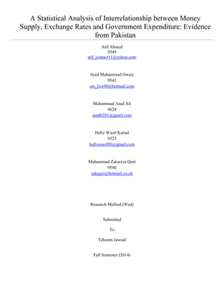
0
10
20
30
40
50
60
70
80
90
100
Year
1972
1975
1978
1981
1984
1987
1990
1993
1996
1999
2002
2005
2008
2011
ExchangeRates
YEAR
Exchange Rate Value
Exchange Rate Value
5. 5
relationship between the size of government and economic growth. Miller and Russek (1997) indicate that debt-
finance increases in government expenditure retarded growth.
It is evident from previous researches that money supply has an impact on government expenditure as
well as economic growth. By taking this hypothesis this research made an attempt to study these variables and
their relationship in Pakistan economy in time period of 1970 to 2012. Also it will investigate that what role is
played by exchange rate in government spending and will try to find out its nature.
0
10
20
30
40
50
60
Year
1971
1973
1975
1977
1979
1981
1983
1985
1987
1989
1991
1993
1995
1997
1999
2001
2003
2005
2007
2009
2011
Moneysupply
YEAR
Money and quasi money (M2) as % of GDP
7. 7
2. Literature Review
2.1.Theoretical Background
The theoretical relationship between government expenditure and money supply and exchange rates is
very important to understand. According to monetarist theory it is assumed that changes in money supply exert a
dominant influence on changing patterns of government expenditure. The public’s demand for money is another
important part of the relationship between money supply and government expenditure1
.
This should be kept in mind that if Rs. 1 bought yesterday what Rs. 2 bought today then there will be a
need for Rs. 2 to sustain the purchasing pattern. That’s why the increased government expenditure is a false
increase in money supply because it is the deficit that government needs to finance, a reserve of money is there
for loans for the government from State Bank of Pakistan and other financial institutions. Now, the exchange rate
is also a major macroeconomic variable that if left ungoverned can be very threatening in fiscal policy making2
.
Literature that was analyzed for this research paper shows little or no sign of exchange rates impacting
government expenditure, which is why this research paper might throw some light on the nature of relationship
between exchange rates and government expenditure.
2.2.Empirical Studies
Sola and Peter (2013) examined the money supply and inflation rate in Nigerian economy. Variables
that were used are inflation rate, money supply, interest rate, exchange rate, oil revenue, and government
expenditure. Time series data has been used for the study purpose from 1970 to 2008. Econometric tests like
Vector Auto-Regression (VAR), Augmented Dickey-Fuller, and Granger Causality were used. A positive
relation between money supply and inflation rate is found also causality test shows unidirectional causality
between exchange rate and inflation rate, interest rate and inflation rate, also money supply and government
expenditures.
Ali et al (2013) enquired the impact of government expenditures on economic growth during different
democratic and dictatorial eras. The data is from the year of 1972-2009. Different sub-categories of government
1
Amedeo Strano (2002)
2
Cakrani et al (2013)
8. 8
expenditures are taken as variables. Data analysis is carried out by using Auto-Regressive Distributed Lag
(ADL). It is concluded that development expenditure heavily support economic growth and it’s also validates the
assumption of that public and private investments are complementary to each other.
Georgantopoulos and Tsamis (2012) investigated the interrelationship of money supply, government
expenditure, prices, and economic growth in both short-run and long-run in Cyprus. For this purpose the variable
used are M2 (broad money), CPI, and Real GDP. Annual data is gathered form year 1980 to 2009. Error Correction
Model (ECM) and Johnson co-integration techniques were used to analyze the data. Findings show that inflation
effects economic growth very badly, and this is recommended to control government expenditures that increase
aggregate demand and shifting of these expenditures to increase aggregate supply.
Husnain et al (2011) questioned the interrelationship of government spending, foreign direct investment,
and economic growth in Pakistan scenario. The data is collect from 1975 to 2008. Four variables were taken for
analyses that are capital (K), labor (L), foreign direct investment (F), and total factor productivity (A). It is
concluded that one most contributing factor in Pakistan’s economic growth is trade openness and the existing
government expenditure structure is not in accordance to the economic needs it must be reorganized.
Mehmood and Sadiq (2010) examined the effect of government expenditure in the form of fiscal deficits on
level tax revenues. Using controlled variables poverty, government expenditure, remittance, private investment, and
secondary school enrollment from 1976 to 2010 annually. For long-run relationship co-integration test is applied and
for short-run error correction model is used. The Augmented Dickey-Fuller results show that poverty reduces due to
public spending thrift and remittances. Also public spending will increase aggregate demand in long-run.
Muhammad et al (2009) examined the relationship among government expenditure, M2, inflation and
economic growth in Pakistan. Data was collected from the year 1977 to 2007. The method used for this purpose was
Johnson co integration test to check the long term relationship, Granger causality test also has been used. The
research findings revealed that there exists a negative relationship b/w public expenditure and inflation with
economic growth. Also M2 is positively related to economic growth. The only reason that was determined for
negative relationship by the research was due to cost push inflation. The research suggested that growth rate of
money supply should be controlled. And governments must try to restrain from financing deficit by borrowing from
central bank.
9. 9
Iqbal and Malik (2009) studied the relationship between government expenditure and taxes for the case of
Pakistan using annual data from 1961 to 2008. The method used Vector Error Correction Model (VECM), granger,
co-integration model, Augmented Dickey-Fuller and Johnson Co-integration approach. The analysis shows that in
case of Pakistan budget deficit and debt have close relationship. But the budget deficits have no impact on the
behavior of government taxes and expenditure in Pakistan. It means in case of Pakistan results found that taxes and
spending decision have no relation and there is no long run co-integration between taxes and expenditure.
Adrison (2002) explained money supply and government expenditure on economic growth in Indonesia
to check the asymmetric effect. Money supply and government expenditures are used as variables to run the
tests. The data collected is quarterly from 1980-1997. The technique that has been used is TARCH (Threshold
Auto Regressive Conditional Heteroscedasticity). The regression model showed that the government expenditure
has an asymmetric effect on economic output and also that money supply is not a contributing factor in inflation.
It is recommended that reallocation of government spending more towards developmental programs.
Albatel (2000) attempted to instigate the relationship between government expenditure and economic
growth in Saudi Arabia. GDP, government expenditure, government consumption, private investment, oil revenues,
and other revenues are variables upon which data is collected from 1964-1995. Method that is used to examine the
data is Augmented Dickey-Fuller (ADF). On the basis of results it is concluded that government should continue
providing economic infrastructure and social activities and on the other hand advise and encourage the private
investors to play a meaningful role as well.
Hsieh and Lai (1994) queried the relationship of government spending and economic growth in G-7
countries. The data is collected on Real GDP and share of government expenditure on goods and services from
1885-1997. Data analysis is done by using ADF and Phillip-PerronZt(q) test. The findings proved that relationship
between government spending and economic growth can vary across time. But still government spending is the only
best way possible for growth in economy.
11. 11
3. Methodology
3.1.Modeling Framework
To estimate the effect of money supply (MS) and exchange rates (ER) on government
expenditure (GE) in Pakistan following model is used:
GE= α + β1MS +β2ER + ε
Hₒ1 = MS does not affect GE
Hₒ2 = ER does not affect GE
Where GE is the percentage of GDP of Gross National Expenditure is taken, MS is taken as Quasi
Money M2 as percentage of GDP and ER is taken as amount in rupees against 1 US dollar; Data for all
research variables is from the time period of 1970 to 2012. Data for research variables under
consideration is taken from World Bank3
.
3
Link address: http://data.worldbank.org/country/pakistan
13. 13
4. Estimation and Result
4.1.1. Estimate Equation (Regression)
Hₒ= MS and ER does not affect GE
Table 1
Variables Coefficient Prob
Constant 124.0585 0.0000
MS -0.367716 0.0079
ER -0.058903 0.0045
It is shown that MS and ER have negative relation with the dependent variable GE, meaning if
MS increase by 1 unit GE will decrease by 0.3167 units and if ER increase by 1 unit than GE will
decrease by 0.0589 units.
4.1.2. Stationary Analysis
So to check the trend in the data stationary analysis is conducted for verification. Unit root test is
used for stationary analysis with Augmented Dickey-Fuller statistic. The hypothesis is that there is a trend
in data or the data is non-stationary.
Unit root test has been performed for all variables with level and 1st
difference, and 2nd
difference is also used where 1st
difference shows the contradiction. The test has been run for individual
intercept and individual intercept & Trend. The results have been reported in table 2.
Table 2
Variables
Level 1st
Difference
C C&T C C&T
GE -2.023248 -2.148364 -6.912705 -6.822305
MS -4.407745 -4.665224 -5.342827 -6.176806
ER 2.933613 -4.665224 -3.839290 -4.988724
14. 14
4.1.3. Heteroskedasticity Test
Heteroskedasticity often arises in cross sectional data but the data taken for the research purpose
is already time series. The P value is 0.121 it means that there is no existence of heteroskedasticity in the
data.
4.1.4. Auto Correlation LM Test
When computed, the resulting number can range from 0 to 4. An autocorrelation of less than 2
represents perfect positive correlation, an increase seen in one time series will lead to a proportionate
increase in the other time series, while a value of greater than 2 represents perfect negative correlation, an
increase seen in one time series results in a proportionate decrease in the other time series4
.
The probability value is 0 it means there exist positive autocorrelation in the data. The removal
of auto correlation can be viewed in appendix.
4
Link address http://www.investopedia.com
Prob 0.121
Heteroscedesticity Test
Table 3
Prob 0.000
Table 4
Breusch-Godfrey Serial Correlation LMTest
15. 15
4.1.5. Stability Test
CUSUM TEST CUSUM SQUARE TEST
CUSUM is the difference between each measurement and the
error value. We can see in the above diagram that the error limit
is ±5%. All the data variable variables are under the significance
level showing that data is stable.
To verify the previous CUSUM SQUARE test is carried out here
we can see that the provided data is crossing the significance
level of 5% somewhere in year 1997 or 1998 which is not
required so as to remove it we take the help of Chow’s breakpoint
test. (see appendix)
4.1.6. Co-integration test
Table 5
Variables
Hypothesis
No. of CE(s)
Trace
Statistics
5% Critical
Values
Maximum
Eigen Value
Statistics
5% Critical
Values
GE MS ER
None * 32.91231 29.79707 23.72303 21.13162
At most 1 9.189281 15.49471 6.234627 14.26460
At most 2 2.954653 3.841466 2.954653 3.841466
* denotes rejection of the hypothesis at the 0.05 level
It is found out that there is no co-integration between the said variables government expenditure, money
supply, and exchange rates. At level “None” the p-value appeared to be 0.0212 or 2.12% less than 5% significance
level. So we reject Hₒ that says variables are co-integrated.
4.1.7. Causality Analysis
Table 6
Null Hypothesis F-Statistics Probability
ER does not Granger Cause GE 0.43866 0.51167
GE does not Granger Cause ER 0.95095 0.33549
-20
-10
0
10
20
1975 1980 1985 1990 1995 2000 2005 2010
CUSUM 5% Significance
-0.4
0.0
0.4
0.8
1.2
1.6
1975 1980 1985 1990 1995 2000 2005 2010
CUSUM of Squares 5% Significance
16. 16
MS does not Granger Cause GE 0.12182 0.72895
GE does not Granger Cause MS 0.82282 0.36993
MS does not Granger Cause ER 0.39045 0.53570
ER does not Granger Cause MS 0.00973 0.92194
It is evident from the causality test that money supply and exchange rates both combined are not
causing government expenditure. But, it is the government expenditure that is causing money supply and
exchange rates.
18. 18
5. Conclusion
On the basis of data analysis the study is able to conclude that money supply and exchange rates are
negatively affecting government expenditure. Using the annual data of the period 1970-2012, we found that there is
negative relationship between money supply and exchange rates on government expenditure in long run.
First of all, we have to understand that change in money supply is not the only way of financing
government spending, but for past several years there has been a lot of pressure given on central bank borrowing,
plus borrowing from international financial institution have rapidly change Pakistan’s economic positions. Secondly
a country’s economic performance can be judged by its exchange rate values, one can realize the fact that the more
rupees depreciate then more money is required by the government to pay the debts and run the economic operations.
Whatever the reason is government must need to curtail its expenses and find some other solutions rather
than burdening it’s on economy. Some of the policy recommendation that government authorities need to consider
are a follow:
1. Government expenditure on infrastructure so as to facilitate the economic growth in the long-term scenario.
2. Developing such financial and capital markets that can mobilize savings and channel them to productive use.
3. Investment should be made in international arena in different assets with the aim of having high return rather
than borrowing from World Bank or other financial bodies.
20. 20
6. References
o Buchanan and Wagner 1977 “Democracy in Deficit”, New York: Academic Press
o Buchanan and Wagner 1978 “Dialogues concerning Fiscal Religion”, Journal of Monetary Economics, vol.4, pp
627-36
o Blackley 1986 “Causality between Revenues and Expenditures and the Size of the Federal Budget” Public Finance
Quarterly, vol.14, pp 139-56
o Ram 1988 “Additional Evidence on Causality between Government Revenue and Government Expenditure”,
Southern Economic Journal vol-54, pp 763-69
o Guffey 1985 “The Federal Reserve’s Role in Promoting Economic Growth”, FRB Kansas city, Economic Review
o Landau 1983 “Government Expenditure and Growth Rate: A Cross Country Study”, Southern Economic Journal,
vol-49, 783-92
o Iqbal an Malik “Budget Balance through Revenue or Spending Adjustment: Evidence from Pakistan”, The Pakistan
Development Review, 49:4 Part II (Winter 2010) pp. 611–630
o Jiranyakul 2007 “The Relation between Government Expenditures and Economic Growth in Thailand”, Munich
Personal RePEc Archive, Paper no 46070
o Mehmood and Sadiq 2010 “The Relationship between Government Expenditure and Poverty: A Cointegration
Analysis”, Romanian Journal of Fiscal Policy, Volume 1, Issue 1, July-December 2010, Pages 29-37
o Hsieh and Lai 1994 “Government spending and Economic Growth: The G-7 Experience”, California State
University, Journal of Applied economics, Vol 26, 535-542
o Adrison 2002 “The Effect of Money Supply and Government Expenditure Shock in Indonesia: Symmetric or
Asymmetric”, International Study Program
o Strano 2002 “How and How much can the money Supply affect the Inflation
Rate”,http://ukdataservice.ac.uk/media/263125/strano-paper.pdf
o Sola and Peter 2013 “Money Supply and Inflation in Nigeria: Implications for National Development”, Modern
Economy, http://www.scrip.org/journal/me, Vol 4, 161-170
o Cakrani et al 2013 “ Government spending and Real Exchange Rate: Case of Albania”, European Journal of
Sustainable Development, Vol 2, Issue 4, 303-310
o Albatel 2000 “The Relationship between Government Expenditure and Economic Growth in Saudi Arabia”,
journal of King Saud University, Vol 2, 173-191
o Georagantopoulas and Tsamis 2010 “The Interrelationship between Money Supply, Prices, Government
Expenditure, and Economic Growth: A Causality Analysis for the Case of Cyprus” International Journal of
Economic Science and Applied Research, Vol 5 (3), 115-128
o Mohammad et al 2009 “An Empirical Investigation between Money Supply, Government Expenditure, Output &
Prices: The Pakistan Evidence”, European Journal of Economics, Finance and Administrative Sciences ISSN 1450-
2275 Issue 17
21. 21
o Husnain et al “Public Spending, Foreign Direct Investment and Economic Growth”, International Research Journal
of Finance and Economics ISSN 1450-2887 Issue 61
o Ali et al 2013 “The composition of public expenditures and economic growth: evidence from
Pakistan", International Journal of Social Economics, Vol. 40 Issue 11, pp.1010 – 1022
26. 26
Table 1: Regression
Dependent Variable: GE
Method: Least Squares
Date: 12/04/14 Time: 17:30
Sample: 1970 2012
Included observations: 43
Variable Coefficient Std. Error t-Statistic Prob.
ER -0.058903 0.019581 -3.008184 0.0045
MS -0.367716 0.131483 -2.796688 0.0079
C 124.0585 5.611903 22.10632 0.0000
R-squared 0.316909 Mean dependent var 106.3723
Adjusted R-squared 0.282755 S.D. dependent var 3.891667
S.E. of regression 3.295865 Akaike info criterion 5.290429
Sum squared resid 434.5090 Schwarz criterion 5.413303
Log likelihood -110.7442 F-statistic 9.278695
Durbin-Watson stat 0.593900 Prob(F-statistic) 0.000489
Table 2: Stationary analysis
GE variable
Level: Intercept
Null Hypothesis: GE has a unit root
Exogenous: Constant
Lag Length: 0 (Automatic based on SIC, MAXLAG=1)
t-Statistic Prob.*
Augmented Dickey-Fuller test statistic -2.023248 0.2761
Test critical values: 1% level -3.596616
5% level -2.933158
10% level -2.604867
*MacKinnon (1996) one-sided p-values.
Augmented Dickey-Fuller Test Equation
Dependent Variable: D(GE)
Method: Least Squares
Date: 12/04/14 Time: 18:14
Sample (adjusted): 1971 2012
Included observations: 42 after adjustments
Variable Coefficient Std. Error t-Statistic Prob.
GE(-1) -0.187393 0.092620 -2.023248 0.0498
C 19.95092 9.855305 2.024384 0.0496
27. 27
R-squared 0.092837 Mean dependent var 0.024488
Adjusted R-squared 0.070158 S.D. dependent var 2.417742
S.E. of regression 2.331387 Akaike info criterion 4.577252
Sum squared resid 217.4147 Schwarz criterion 4.659998
Log likelihood -94.12229 Hannan-Quinn criter. 4.607582
F-statistic 4.093532 Durbin-Watson stat 1.998466
Prob(F-statistic) 0.049766
Level: Trend and Intercept
Null Hypothesis: GE has a unit root
Exogenous: Constant, Linear Trend
Lag Length: 0 (Automatic - based on SIC, maxlag=1)
t-Statistic Prob.*
Augmented Dickey-Fuller test statistic -2.148364 0.5048
Test critical values: 1% level -4.192337
5% level -3.520787
10% level -3.191277
*MacKinnon (1996) one-sided p-values.
Augmented Dickey-Fuller Test Equation
Dependent Variable: D(GE)
Method: Least Squares
Date: 12/17/14 Time: 19:59
Sample (adjusted): 1971 2012
Included observations: 42 after adjustments
Variable Coefficient Std. Error t-Statistic Prob.
GE(-1) -0.226091 0.105239 -2.148364 0.0380
C 24.63691 11.55258 2.132590 0.0393
@TREND("1970") -0.026558 0.033723 -0.787544 0.4357
R-squared 0.107038 Mean dependent var 0.024488
Adjusted R-squared 0.061246 S.D. dependent var 2.417742
S.E. of regression 2.342534 Akaike info criterion 4.609093
Sum squared resid 214.0112 Schwarz criterion 4.733212
Log likelihood -93.79095 Hannan-Quinn criter. 4.654588
F-statistic 2.337446 Durbin-Watson stat 1.955270
Prob(F-statistic) 0.109961
1st
Difference: Intercept
Null Hypothesis: D(GE) has a unit root
Exogenous: Constant
Lag Length: 0 (Automatic based on SIC, MAXLAG=1)
t-Statistic Prob.*
Augmented Dickey-Fuller test statistic -6.912705 0.0000
Test critical values: 1% level -3.600987
28. 28
5% level -2.935001
10% level -2.605836
*MacKinnon (1996) one-sided p-values.
Augmented Dickey-Fuller Test Equation
Dependent Variable: D(GE,2)
Method: Least Squares
Date: 12/04/14 Time: 18:19
Sample (adjusted): 1972 2012
Included observations: 41 after adjustments
Variable Coefficient Std. Error t-Statistic Prob.
D(GE(-1)) -1.116067 0.161452 -6.912705 0.0000
C 0.050291 0.383336 0.131193 0.8963
R-squared 0.550616 Mean dependent var 0.101927
Adjusted R-squared 0.539093 S.D. dependent var 3.614790
S.E. of regression 2.454084 Akaike info criterion 4.680935
Sum squared resid 234.8786 Schwarz criterion 4.764524
Log likelihood -93.95917 Hannan-Quinn criter. 4.711373
F-statistic 47.78549 Durbin-Watson stat 2.024600
Prob(F-statistic) 0.000000
1st
Difference: Trend and Intercept
Null Hypothesis: D(GE) has a unit root
Exogenous: Constant, Linear Trend
Lag Length: 0 (Automatic - based on SIC, maxlag=1)
t-Statistic Prob.*
Augmented Dickey-Fuller test statistic -6.822305 0.0000
Test critical values: 1% level -4.198503
5% level -3.523623
10% level -3.192902
*MacKinnon (1996) one-sided p-values.
Augmented Dickey-Fuller Test Equation
Dependent Variable: D(GE,2)
Method: Least Squares
Date: 12/17/14 Time: 20:00
Sample (adjusted): 1972 2012
Included observations: 41 after adjustments
Variable Coefficient Std. Error t-Statistic Prob.
D(GE(-1)) -1.115871 0.163562 -6.822305 0.0000
C -0.011621 0.819646 -0.014178 0.9888
@TREND("1970") 0.002815 0.032815 0.085771 0.9321
R-squared 0.550703 Mean dependent var 0.101927
29. 29
Adjusted R-squared 0.527056 S.D. dependent var 3.614790
S.E. of regression 2.485924 Akaike info criterion 4.729522
Sum squared resid 234.8332 Schwarz criterion 4.854905
Log likelihood -93.95520 Hannan-Quinn criter. 4.775180
F-statistic 23.28829 Durbin-Watson stat 2.025199
Prob(F-statistic) 0.000000
MS variable
Level: Intercept
Null Hypothesis: MS has a unit root
Exogenous: Constant
Lag Length: 1 (Automatic - based on SIC, maxlag=1)
t-Statistic Prob.*
Augmented Dickey-Fuller test statistic -4.407745 0.0011
Test critical values: 1% level -3.600987
5% level -2.935001
10% level -2.605836
*MacKinnon (1996) one-sided p-values.
Augmented Dickey-Fuller Test Equation
Dependent Variable: D(MS)
Method: Least Squares
Date: 12/17/14 Time: 20:02
Sample (adjusted): 1972 2012
Included observations: 41 after adjustments
Variable Coefficient Std. Error t-Statistic Prob.
MS(-1) -0.552360 0.125316 -4.407745 0.0001
D(MS(-1)) 0.453209 0.145532 3.114156 0.0035
C 23.49588 5.380859 4.366567 0.0001
R-squared 0.355535 Mean dependent var -0.167054
Adjusted R-squared 0.321615 S.D. dependent var 3.385277
S.E. of regression 2.788253 Akaike info criterion 4.959063
Sum squared resid 295.4256 Schwarz criterion 5.084447
Log likelihood -98.66080 Hannan-Quinn criter. 5.004721
F-statistic 10.48180 Durbin-Watson stat 1.952386
Prob(F-statistic) 0.000237
Level: Trend and Intercept
Null Hypothesis: MS has a unit root
Exogenous: Constant, Linear Trend
Lag Length: 1 (Automatic - based on SIC, maxlag=1)
t-Statistic Prob.*
Augmented Dickey-Fuller test statistic -4.665224 0.0029
30. 30
Test critical values: 1% level -4.198503
5% level -3.523623
10% level -3.192902
*MacKinnon (1996) one-sided p-values.
Augmented Dickey-Fuller Test Equation
Dependent Variable: D(MS)
Method: Least Squares
Date: 12/17/14 Time: 20:04
Sample (adjusted): 1972 2012
Included observations: 41 after adjustments
Variable Coefficient Std. Error t-Statistic Prob.
MS(-1) -0.597087 0.127987 -4.665224 0.0000
D(MS(-1)) 0.487622 0.145949 3.341049 0.0019
C 24.26573 5.346348 4.538748 0.0001
@TREND("1970") 0.052086 0.037651 1.383389 0.1748
R-squared 0.387229 Mean dependent var -0.167054
Adjusted R-squared 0.337545 S.D. dependent var 3.385277
S.E. of regression 2.755322 Akaike info criterion 4.957414
Sum squared resid 280.8967 Schwarz criterion 5.124592
Log likelihood -97.62698 Hannan-Quinn criter. 5.018291
F-statistic 7.793820 Durbin-Watson stat 2.027069
Prob(F-statistic) 0.000372
1st
difference: Intercept
Null Hypothesis: D(MS) has a unit root
Exogenous: Constant
Lag Length: 0 (Automatic based on SIC, MAXLAG=9)
t-Statistic Prob.*
Augmented Dickey-Fuller test statistic -5.342827 0.0001
Test critical values: 1% level -3.600987
5% level -2.935001
10% level -2.605836
*MacKinnon (1996) one-sided p-values.
Augmented Dickey-Fuller Test Equation
Dependent Variable: D(MS,2)
Method: Least Squares
Date: 12/04/14 Time: 18:23
Sample (adjusted): 1972 2012
Included observations: 41 after adjustments
Variable Coefficient Std. Error t-Statistic Prob.
D(MS(-1)) -0.839546 0.157135 -5.342827 0.0000
C -0.143632 0.528907 -0.271564 0.7874
31. 31
R-squared 0.422614 Mean dependent var -0.021079
Adjusted R-squared 0.407809 S.D. dependent var 4.396750
S.E. of regression 3.383472 Akaike info criterion 5.323232
Sum squared resid 446.4674 Schwarz criterion 5.406821
Log likelihood -107.1263 Hannan-Quinn criter. 5.353671
F-statistic 28.54580 Durbin-Watson stat 1.877839
Prob(F-statistic) 0.000004
1st
Difference: Trend and Intercept
Null Hypothesis: D(MS) has a unit root
Exogenous: Constant, Linear Trend
Lag Length: 1 (Automatic - based on SIC, maxlag=1)
t-Statistic Prob.*
Augmented Dickey-Fuller test statistic -6.176806 0.0000
Test critical values: 1% level -4.205004
5% level -3.526609
10% level -3.194611
*MacKinnon (1996) one-sided p-values.
Augmented Dickey-Fuller Test Equation
Dependent Variable: D(MS,2)
Method: Least Squares
Date: 12/17/14 Time: 20:05
Sample (adjusted): 1973 2012
Included observations: 40 after adjustments
Variable Coefficient Std. Error t-Statistic Prob.
D(MS(-1)) -1.191044 0.192825 -6.176806 0.0000
D(MS(-1),2) 0.393181 0.151120 2.601788 0.0134
C -0.772192 1.092379 -0.706890 0.4842
@TREND("1970") 0.022737 0.043197 0.526346 0.6019
R-squared 0.536170 Mean dependent var -0.052523
Adjusted R-squared 0.497518 S.D. dependent var 4.448090
S.E. of regression 3.153072 Akaike info criterion 5.229271
Sum squared resid 357.9071 Schwarz criterion 5.398159
Log likelihood -100.5854 Hannan-Quinn criter. 5.290335
F-statistic 13.87157 Durbin-Watson stat 1.961720
Prob(F-statistic) 0.000004
ER variable
Level: Intercept
Null Hypothesis: ER has a unit root
Exogenous: Constant
Lag Length: 0 (Automatic based on SIC, MAXLAG=1)
t-Statistic Prob.*
32. 32
Augmented Dickey-Fuller test statistic 2.933613 1.0000
Test critical values: 1% level -3.596616
5% level -2.933158
10% level -2.604867
*MacKinnon (1996) one-sided p-values.
Augmented Dickey-Fuller Test Equation
Dependent Variable: D(ER)
Method: Least Squares
Date: 12/05/14 Time: 07:40
Sample (adjusted): 1971 2012
Included observations: 42 after adjustments
Variable Coefficient Std. Error t-Statistic Prob.
ER(-1) 0.048655 0.016585 2.933613 0.0055
C 0.531435 0.673102 0.789531 0.4345
R-squared 0.177058 Mean dependent var 2.110476
Adjusted R-squared 0.156484 S.D. dependent var 2.851876
S.E. of regression 2.619252 Akaike info criterion 4.810102
Sum squared resid 274.4191 Schwarz criterion 4.892848
Log likelihood -99.01215 F-statistic 8.606083
Durbin-Watson stat 1.445382 Prob(F-statistic) 0.005524
Level: Trend and Intercept
Null Hypothesis: ER has a unit root
Exogenous: Constant, Linear Trend
Lag Length: 0 (Automatic - based on SIC, maxlag=1)
t-Statistic Prob.*
Augmented Dickey-Fuller test statistic -0.258601 0.9894
Test critical values: 1% level -4.192337
5% level -3.520787
10% level -3.191277
*MacKinnon (1996) one-sided p-values.
Augmented Dickey-Fuller Test Equation
Dependent Variable: D(ER)
Method: Least Squares
Date: 12/17/14 Time: 20:08
Sample (adjusted): 1971 2012
Included observations: 42 after adjustments
33. 33
Variable Coefficient Std. Error t-Statistic Prob.
ER(-1) -0.013444 0.051989 -0.258601 0.7973
C -0.283093 0.930000 -0.304401 0.7624
@TREND("1970") 0.131623 0.104522 1.259287 0.2154
R-squared 0.209212 Mean dependent var 2.110476
Adjusted R-squared 0.168659 S.D. dependent var 2.851876
S.E. of regression 2.600280 Akaike info criterion 4.817865
Sum squared resid 263.6968 Schwarz criterion 4.941984
Log likelihood -98.17516 Hannan-Quinn criter. 4.863359
F-statistic 5.158962 Durbin-Watson stat 1.417172
Prob(F-statistic) 0.010284
1st
Difference: Intercept
Null Hypothesis: D(ER) has a unit root
Exogenous: Constant
Lag Length: 0 (Automatic based on SIC, MAXLAG=1)
t-Statistic Prob.*
Augmented Dickey-Fuller test statistic -3.839290 0.0053
Test critical values: 1% level -3.600987
5% level -2.935001
10% level -2.605836
*MacKinnon (1996) one-sided p-values.
Augmented Dickey-Fuller Test Equation
Dependent Variable: D(ER,2)
Method: Least Squares
Date: 12/05/14 Time: 07:42
Sample (adjusted): 1972 2012
Included observations: 41 after adjustments
Variable Coefficient Std. Error t-Statistic Prob.
D(ER(-1)) -0.580057 0.151084 -3.839290 0.0004
C 1.326366 0.511912 2.591006 0.0134
R-squared 0.274286 Mean dependent var 0.172195
Adjusted R-squared 0.255678 S.D. dependent var 3.075190
S.E. of regression 2.653093 Akaike info criterion 4.836880
Sum squared resid 274.5172 Schwarz criterion 4.920469
Log likelihood -97.15604 F-statistic 14.74015
Durbin-Watson stat 1.733545 Prob(F-statistic) 0.000441
34. 34
1st
Difference: Trend and Intercept
Null Hypothesis: D(ER) has a unit root
Exogenous: Constant, Linear Trend
Lag Length: 1 (Automatic - based on SIC, maxlag=1)
t-Statistic Prob.*
Augmented Dickey-Fuller test statistic -4.988724 0.0012
Test critical values: 1% level -4.205004
5% level -3.526609
10% level -3.194611
*MacKinnon (1996) one-sided p-values.
Augmented Dickey-Fuller Test Equation
Dependent Variable: D(ER,2)
Method: Least Squares
Date: 12/17/14 Time: 20:10
Sample (adjusted): 1973 2012
Included observations: 40 after adjustments
Variable Coefficient Std. Error t-Statistic Prob.
D(ER(-1)) -0.930109 0.186442 -4.988724 0.0000
D(ER(-1),2) 0.303859 0.160752 1.890238 0.0668
C -0.683185 0.832711 -0.820435 0.4174
@TREND("1970") 0.117774 0.037899 3.107564 0.0037
R-squared 0.431053 Mean dependent var 0.078500
Adjusted R-squared 0.383641 S.D. dependent var 3.054524
S.E. of regression 2.398062 Akaike info criterion 4.681838
Sum squared resid 207.0252 Schwarz criterion 4.850726
Log likelihood -89.63676 Hannan-Quinn criter. 4.742903
F-statistic 9.091606 Durbin-Watson stat 1.864814
Prob(F-statistic) 0.000129
Table 3
Heteroscedesticity Test
White Heteroskedasticity Test:
F-statistic 1.884473 Probability 0.120651
Obs*R-squared 8.727726 Probability 0.120430
Test Equation:
Dependent Variable: RESID^2
Method: Least Squares
Date: 12/04/14 Time: 17:35
Sample: 1970 2012
Included observations: 43
35. 35
Variable Coefficient Std. Error t-Statistic Prob.
C -228.0955 168.4667 -1.353950 0.1840
ER 0.810815 1.084077 0.747931 0.4592
ER^2 -0.005374 0.003680 -1.460195 0.1527
ER*MS -0.005402 0.020903 -0.258439 0.7975
MS 11.18316 7.991880 1.399315 0.1700
MS^2 -0.135581 0.094344 -1.437096 0.1591
R-squared 0.202970 Mean dependent var 10.10486
Adjusted R-squared 0.095264 S.D. dependent var 11.17521
S.E. of regression 10.62959 Akaike info criterion 7.693948
Sum squared resid 4180.563 Schwarz criterion 7.939697
Log likelihood -159.4199 F-statistic 1.884473
Durbin-Watson stat 1.824780 Prob(F-statistic) 0.120651
Table 4
Auto-Correlation LM Test
Breusch-Godfrey Serial Correlation LM Test:
F-statistic 37.80496 Probability 0.000000
Obs*R-squared 21.16547 Probability 0.000004
Test Equation:
Dependent Variable: RESID
Method: Least Squares
Date: 12/04/14 Time: 17:37
Presample missing value lagged residuals set to zero.
Variable Coefficient Std. Error t-Statistic Prob.
ER 0.003985 0.014146 0.281704 0.7797
MS 0.060006 0.095387 0.629077 0.5330
C -2.627672 4.072397 -0.645240 0.5226
RESID(-1) 0.720410 0.117167 6.148574 0.0000
R-squared 0.492220 Mean dependent var -7.44E-15
Adjusted R-squared 0.453160 S.D. dependent var 3.216435
S.E. of regression 2.378509 Akaike info criterion 4.659233
Sum squared resid 220.6349 Schwarz criterion 4.823065
Log likelihood -96.17350 F-statistic 12.60165
Durbin-Watson stat 1.972120 Prob(F-statistic) 0.000007
36. 36
Chow Breakpoint Test
Chow Breakpoint Test: 1998
F-statistic 5.693700 Probability 0.002614
Log likelihood ratio 16.32138 Probability 0.000974
Chow Breakpoint Test: 1999
F-statistic 5.655231 Probability 0.002713
Log likelihood ratio 16.22952 Probability 0.001017
Table 5
Co-integration Test
Date: 12/17/14 Time: 21:19
Sample (adjusted): 1972 2012
Included observations: 41 after adjustments
Trend assumption: Linear deterministic trend
Series: GE MS ER
Lags interval (in first differences): 1 to 1
Unrestricted Cointegration Rank Test (Trace)
Hypothesized Trace 0.05
No. of CE(s) Eigenvalue Statistic Critical Value Prob.**
None * 0.439323 32.91231 29.79707 0.0212
At most 1 0.141067 9.189281 15.49471 0.3482
At most 2 0.069529 2.954653 3.841466 0.0856
Trace test indicates 1 cointegratingeqn(s) at the 0.05 level
* denotes rejection of the hypothesis at the 0.05 level
**MacKinnon-Haug-Michelis (1999) p-values
Unrestricted Cointegration Rank Test (Maximum Eigenvalue)
Hypothesized Max-Eigen 0.05
No. of CE(s) Eigenvalue Statistic Critical Value Prob.**
None * 0.439323 23.72303 21.13162 0.0211
At most 1 0.141067 6.234627 14.26460 0.5833
At most 2 0.069529 2.954653 3.841466 0.0856
Max-eigenvalue test indicates 1 cointegratingeqn(s) at the 0.05 level
* denotes rejection of the hypothesis at the 0.05 level
**MacKinnon-Haug-Michelis (1999) p-values
Unrestricted Cointegrating Coefficients (normalized by b'*S11*b=I):
GE MS ER
0.117424 0.323591 0.006315
38. 38
Table 6
Granger’s Causality Test
Pairwise Granger Causality Tests
Date: 12/04/14 Time: 17:56
Sample: 1970 2012
Lags: 1
Null Hypothesis: Obs F-Statistic Probability
ER does not Granger Cause GE 42 0.43866 0.51167
GE does not Granger Cause ER 0.95095 0.33549
MS does not Granger Cause GE 42 0.12182 0.72895
GE does not Granger Cause MS 0.82282 0.36993
MS does not Granger Cause ER 42 0.39045 0.53570
ER does not Granger Cause MS 0.00973 0.92194