Downloaded 42 times


![introduction problem formulation
deterministic observer solution
stochastic observer examples and exercises
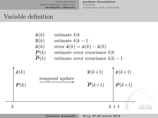
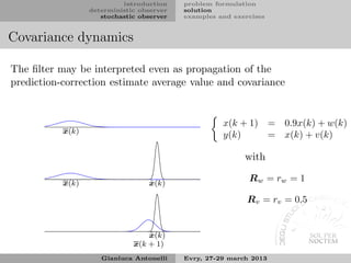
Definitions on stochastic variables I
Given a stochastic variabile x ∈ Rn with probability density
function fx (x) its expected value (average) is
E[x] = µx = xfx (x)dx ∈ Rn
Rn
The covariance matrix is defined as
P x = E (x − µx )(x − µx )T ∈ Rn×n
Gianluca Antonelli Evry, 27-29 march 2013](https://image.slidesharecdn.com/stateestimate-130322032037-phpapp01/85/State-estimate-31-320.jpg)
![introduction problem formulation
deterministic observer solution
stochastic observer examples and exercises
Linear model
Let us consider first the stationary linear model
x(k + 1) = Ax(k) + Bu(k) + w(k)
y(k) = Cx(k) + v(k)
where
E[w(k)] = 0
E[v(k)] = 0
E[w(i)w(j)T ] = Rw δ(i − j) con Rw > O
E[v(i)v(j)T ] = Rv δ(i − j) con Rv > O
E[wh (i)vl (j)] = 0 per ogni i, j, h, l
E[xh (i)vl (j)] = 0 per ogni i, j, h, l
Gianluca Antonelli Evry, 27-29 march 2013](https://image.slidesharecdn.com/stateestimate-130322032037-phpapp01/85/State-estimate-35-320.jpg)
![introduction problem formulation
deterministic observer solution
stochastic observer examples and exercises
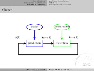
Kalman filter equations
temporal update x(k + 1)
= Aˆ (k) + Bu(k)
x
(prediction)
P (k + 1)
= AP (k)AT + Rw
−1
measurement update K(k) = P (k)C T Rv + CP (k)C T
(correction) ˆ
x(k)
= x(k) + K(k) [y(k) − Cx(k)]
P (k) = P (k) − K(k)CP (k)
Update equations not necessarily synchronous
Possibility to fuse/merge different measurement sources
Suitable to be implemented for the non stationary case
Gianluca Antonelli Evry, 27-29 march 2013](https://image.slidesharecdn.com/stateestimate-130322032037-phpapp01/85/State-estimate-37-320.jpg)
![introduction problem formulation
deterministic observer solution
stochastic observer examples and exercises
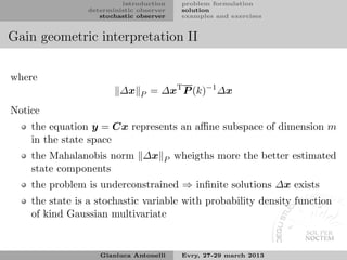
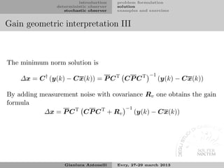
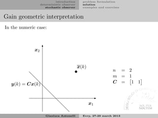
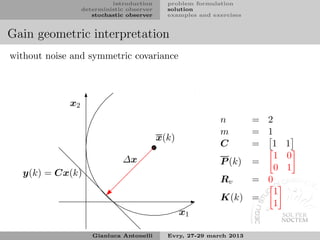
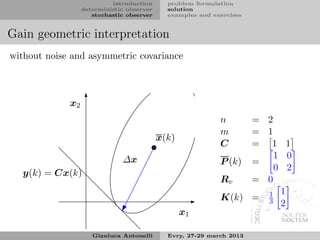
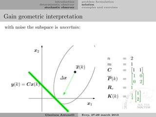
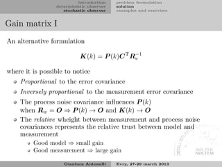
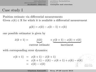
Gain geometric interpretation I
Let us formulate a geometric interpretation of the term
∆x = K(k) [y(k) − Cx(k)]
that appears in the measurement update
ˆ
x(k) = x(k) + K(k) [y(k) − Cx(k)] = x(k) + ∆x
From the output equation we have
y(k) = C (x(k) + ∆x) + v(k)
assuming first absence of noise, it allows to write the following
minimization problem
min ∆x P s.t. C∆x = y(k) − Cx(k)
Gianluca Antonelli Evry, 27-29 march 2013](https://image.slidesharecdn.com/stateestimate-130322032037-phpapp01/85/State-estimate-39-320.jpg)
![introduction problem formulation
deterministic observer solution
stochastic observer examples and exercises
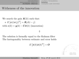
The optimum transient observer
We search the gain K(k) such that:
ˆ
E[x − x] = 0
P (k) minimum
⇓
The solution is formally equal to the Kalman filter
Gianluca Antonelli Evry, 27-29 march 2013](https://image.slidesharecdn.com/stateestimate-130322032037-phpapp01/85/State-estimate-49-320.jpg)
![introduction problem formulation
deterministic observer solution
stochastic observer examples and exercises
Stability
The state estimate evolves following the dynamics
ˆ ˆ
x(k) = (A − K(k)CA) x(k − 1)
An anlytical proof requires hard constraints
When the system is observable E[˜ (k)] is bounded ∀k
x
Stable for most of practical applications
Gianluca Antonelli Evry, 27-29 march 2013](https://image.slidesharecdn.com/stateestimate-130322032037-phpapp01/85/State-estimate-51-320.jpg)
![introduction problem formulation
deterministic observer solution
stochastic observer examples and exercises
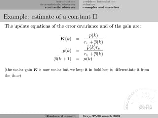
Example: estimate of a constant I
We have at disposal the noisy measurement of a constant with trivial
dynamic
x(k + 1) = x(k) no noise ⇒ (I trust the model!)
y(k) = x(k) + v(k)
where A = 1, H = 1 e E[v(i)v(j)] = rv δ(i − j)
The covariance matrix is given P (0) = p(0) = p0
Gianluca Antonelli Evry, 27-29 march 2013](https://image.slidesharecdn.com/stateestimate-130322032037-phpapp01/85/State-estimate-52-320.jpg)
![introduction problem formulation
deterministic observer solution
stochastic observer examples and exercises
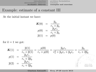
Example: estimate of a constant IV
by iteration it is possible to compute symbolically the gain as
p0 p0 /rv
K(k) = =
rv + (k + 1)p0 1 + (k + 1)p0 /rv
the estimate is then given by:
p0 /rv
x(k) = x(k) +
ˆ [y(k) − x(k)]
1 + (k + 1)p0 /rv
where we notice
for increasing k, the new measurements are not used anymore to
update the estimate
the gain is strongly affected by the ration between p0 and rv
to avoid that the gain tends to zero it is necessary to introduce a
process noise
Gianluca Antonelli Evry, 27-29 march 2013](https://image.slidesharecdn.com/stateestimate-130322032037-phpapp01/85/State-estimate-55-320.jpg)
![introduction problem formulation
deterministic observer solution
stochastic observer examples and exercises
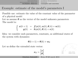
Extended Kalman filter
Idea: we use the nonlinear function whenever possible, otherwise we
use the Jacobians (dynamics linearization):
ˆ
C(k) = ∂
∂ x h(x) x=x(k)
ˆ
A(k) = ∂
∂ x f (x) x=x(k)
ˆ
−1
K(k) ˆ ˆ ˆ
= P (k)C(k)T Rv + C(k)P (k)C(k)T
ˆ
x(k) = x(k) + K(k) [y(k) − h(x(k), k)]
P (k) = ˆ
P (k) − K(k)C(k)P (k)
x(k + 1) = f (ˆ (k), k) + Bu(k)
x
P (k + 1) = ˆ ˆ
A(k)P (k)A(k)T + Rw
Gianluca Antonelli Evry, 27-29 march 2013](https://image.slidesharecdn.com/stateestimate-130322032037-phpapp01/85/State-estimate-56-320.jpg)
![introduction problem formulation
deterministic observer solution
stochastic observer examples and exercises
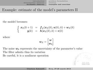
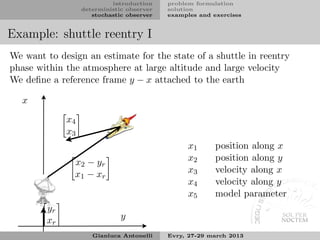
Example: shuttle reentry V
6500
Simulated reentry path
6480
6460
6440
x [km]
6420
6400
6380 radar
6360
6340
6320
6300
-50 0 50 100 150 200 250 300 350
y [km]
Gianluca Antonelli Evry, 27-29 march 2013](https://image.slidesharecdn.com/stateestimate-130322032037-phpapp01/85/State-estimate-63-320.jpg)
![introduction problem formulation
deterministic observer solution
stochastic observer examples and exercises
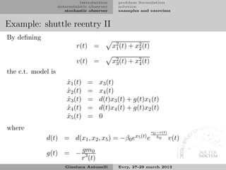
Example: shuttle reentry VI
400
radar measurement
350
y1 [km]
300
250
200
150
100
50
0
0 20 40 60 80 100 120 140 160 180 200
1.4
y2 [rad]
1.3
1.2
1.1
1.0
0 20 40 60 80 100 120 140 160 180 200
t [s]
Gianluca Antonelli Evry, 27-29 march 2013](https://image.slidesharecdn.com/stateestimate-130322032037-phpapp01/85/State-estimate-64-320.jpg)
![introduction problem formulation
deterministic observer solution
stochastic observer examples and exercises
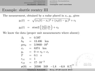
Example: shuttle reentry VII
Simulated reentry path (black) and estimated (red)
6500
6480
6460
6440
x [km]
6420
6400
6380 radar
6360
6340
6320
6300
-50 0 50 100 150 200 250 300 350
y [km]
Gianluca Antonelli Evry, 27-29 march 2013](https://image.slidesharecdn.com/stateestimate-130322032037-phpapp01/85/State-estimate-65-320.jpg)
![introduction problem formulation
deterministic observer solution
stochastic observer examples and exercises
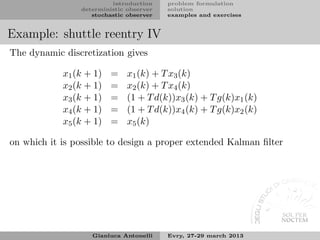
Example: shuttle reentry VIII
6520
x1 350
x2
6500
300
x [km]
y [km]
6480
250
6460
200
6440
150
6420
6400 100
6380 50
0 20 40 60 80 100 120 140 160 180 200 0 20 40 60 80 100 120 140 160 180 200
1
x3 , x4 0.625
x5 (only estimate)
x3 ,x4 [km/s]
0
0.620
-1
0.615
-2 x5 [-]
-3 0.610
-4
0.605
-5
0.600
-6
-7 0.595
0 20 40 60 80 100 120 140 160 180 200 0 20 40 60 80 100 120 140 160 180 200
t [s]
Gianluca Antonelli Evry, 27-29 march 2013](https://image.slidesharecdn.com/stateestimate-130322032037-phpapp01/85/State-estimate-66-320.jpg)
![introduction problem formulation
deterministic observer solution
stochastic observer examples and exercises
Example: shuttle reentry IX
x1 ,x2 ,x3 ,x4 ,x5 , [km],[km/s],[-]
3
˜
x(k)
2
1
0
-1
-2
-3
-4
-5
0 20 40 60 80 100 120 140 160 180 200
t [s]
Numerical example taken from: Austin, JW and Leondes, CT, Statistically
linearized estimation of reentry trajectories, Aerospace and Electronic Systems,
IEEE Transactions on, (1)54–61, 1981
Gianluca Antonelli Evry, 27-29 march 2013](https://image.slidesharecdn.com/stateestimate-130322032037-phpapp01/85/State-estimate-67-320.jpg)
![introduction problem formulation
deterministic observer solution
stochastic observer examples and exercises
Kalman vs Luenberger
Luenberger is based on the deterministic model
In Luenberger we design the estimate convergence speed
Different interpretation of models/data
At steady state they are simbolically equal. When K(k) = K,
Kalman becomes
x(k + 1)
= Aˆ (k) + Bu(k)
x
P (k + 1)
= P
K(k) = K
ˆ
x(k)
= x(k) + K [y(k) − Cx(k)]
P (k) = P
thus
ˆ ˆ
x(k + 1) = Aˆ (k) + Bu(k) + K [y(k) − y (k)]
x
Gianluca Antonelli Evry, 27-29 march 2013](https://image.slidesharecdn.com/stateestimate-130322032037-phpapp01/85/State-estimate-68-320.jpg)
![introduction problem formulation
deterministic observer solution
stochastic observer examples and exercises
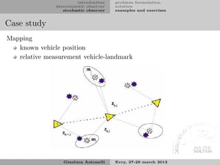
Case study II
The error is thus a Brownian movement (random walking)
e(k + 1) = e(k) + v(k)
E[e(0)] = 0
E[e2 (0)] = 0
E[e2 (1)] = E[(e(0) + v(0))2 ]
= E[e2 (0) + 2e(0)v(0) + v 2 (0)]
2
= rv
E[e (2)] = E[(e(1) + v(1))2 ]
2
= E[e2 (1) + 2e(1)v(1) + v 2 (1)]
2
= 2rv
.
.
.
E[e2 (k)] = krv
2
the variance grows!
Gianluca Antonelli Evry, 27-29 march 2013](https://image.slidesharecdn.com/stateestimate-130322032037-phpapp01/85/State-estimate-70-320.jpg)
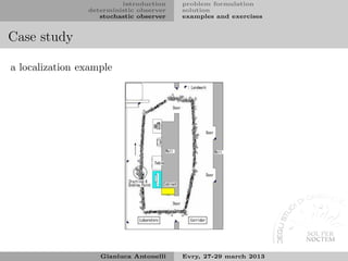
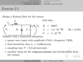
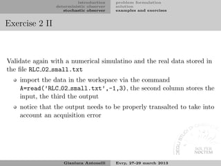


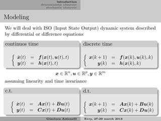
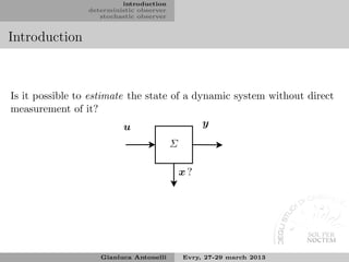
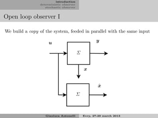
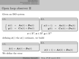
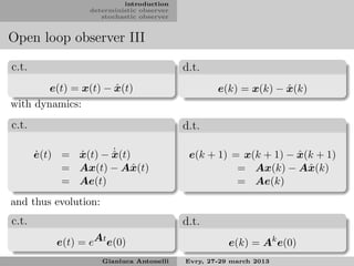
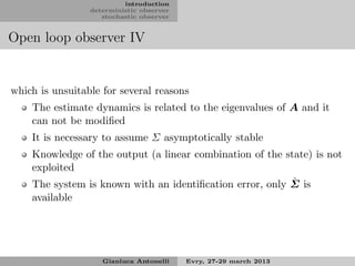
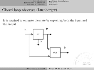
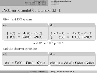
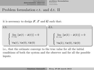
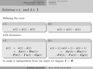
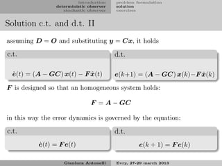
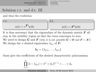
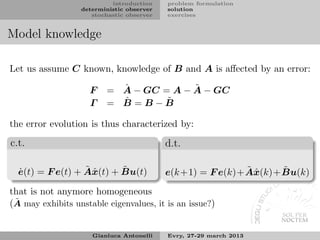
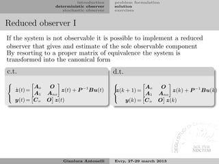
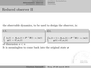
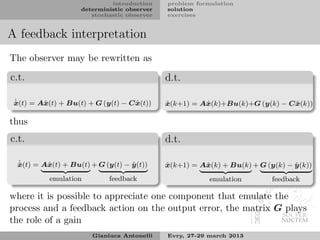
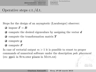
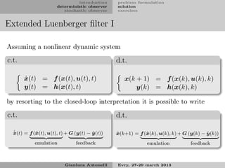
The document introduces deterministic and stochastic observers. Deterministic observers estimate states using a model and measurements, like the Luenberger observer. Stochastic observers, like the Kalman filter, also account for noise. The document discusses open-loop and closed-loop observer designs, how to select observer eigenvalues, and approaches for partial state estimation.