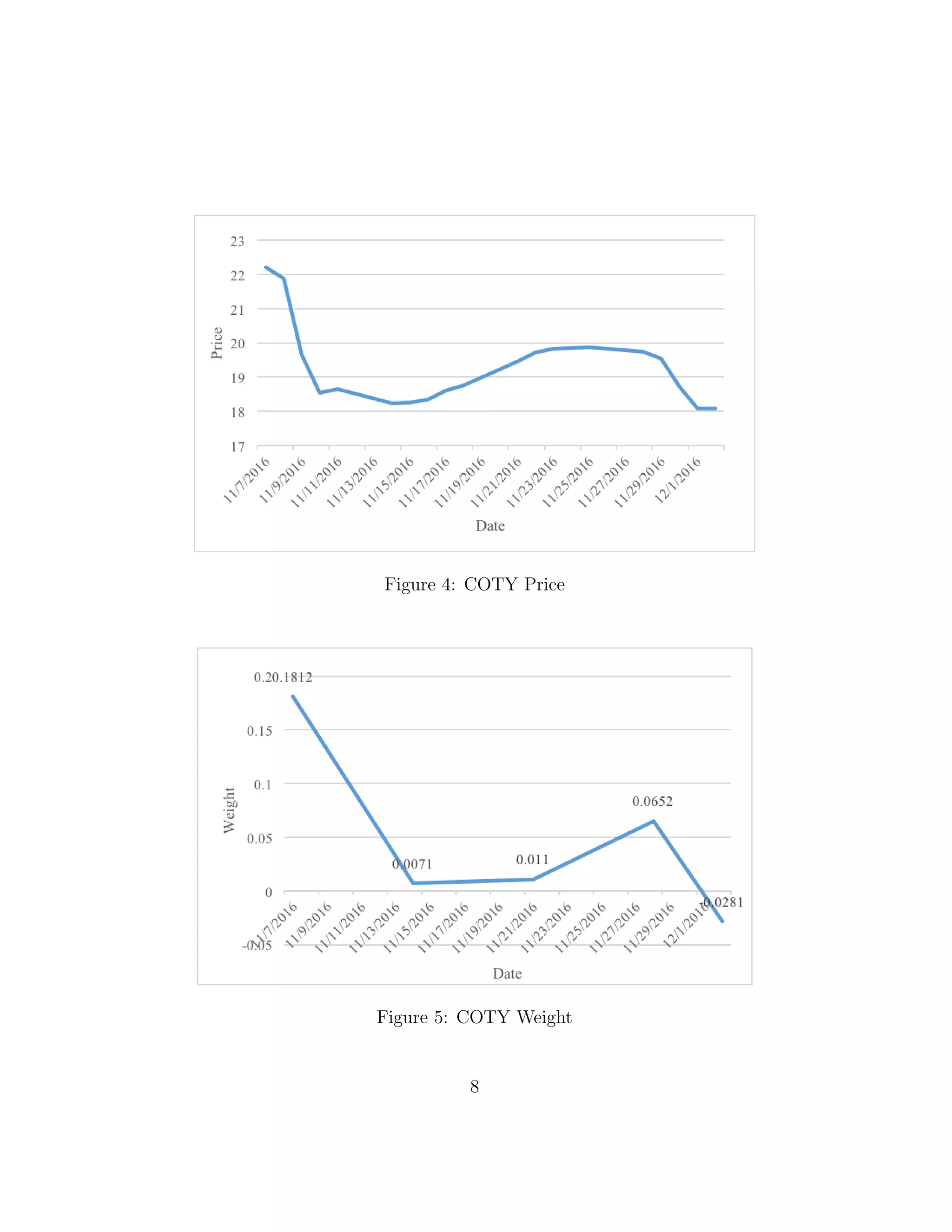
This document is a portfolio optimization project report submitted by Tingwen Zhou and Xuan Ning to Professor Marcel Y. Blais on December 15, 2016. It analyzes the performance of a portfolio reconstructed on November 7, 2016 using a 3-year period of asset data. The portfolio underperformed, losing a total of $86,025. Various metrics are calculated to evaluate the portfolio such as Sharpe ratio, Treynor ratio, and maximum drawdown. The efficient frontier is analyzed over time as weights were rebalanced weekly.

1. Worcester Polytechnic Institute
Financial Mathematics
PORTFOLIO VALUATION AND RISK
MANAGEMENT
Portfolio Optimization Project
Report
Supervisor: Professor Marcel Y. Blais
Author: Tingwen Zhou; Xuan Ning
December 15, 2016

2. Contents
1 Portfolio Reconstruction 3
2 Portfolio Performance 4
2.1 Portfolio value . . . . . . . . . . . . . . . . . . . . . . . . . . . 4
2.2 Efficient frontier (Minimum variance portfolio) . . . . . . . . . 4
2.3 Rebalancing process . . . . . . . . . . . . . . . . . . . . . . . 5
2.4 Change of returns covariance matrix . . . . . . . . . . . . . . 6
2.5 Overall performance . . . . . . . . . . . . . . . . . . . . . . . 7
3 Portfolio Performance Analysis 7
3.1 Sharpe ratio . . . . . . . . . . . . . . . . . . . . . . . . . . . 7
3.2 Treynor ratio . . . . . . . . . . . . . . . . . . . . . . . . . . . 9
3.3 Information ratio . . . . . . . . . . . . . . . . . . . . . . . . . 9
3.4 Sortino ratio . . . . . . . . . . . . . . . . . . . . . . . . . . . . 9
3.5 Maximum drawdown . . . . . . . . . . . . . . . . . . . . . . . 9
3.6 Alpha and beta . . . . . . . . . . . . . . . . . . . . . . . . . . 10
3.7 Comparison of the portfolio performance to S&P 500 . . . . . 10
3.8 Margin calls . . . . . . . . . . . . . . . . . . . . . . . . . . . . 11
4 Leverage Analysis 12
5 Conclusions 12
6 Factor Modeling 14
6.1 Fit the returns distribution to both a normal and a t density . 14
6.2 Perform a goodness-of-fit hypothesis test . . . . . . . . . . . . 14
Appendices 16
1

3. List of Figures
1 Portfolio Value . . . . . . . . . . . . . . . . . . . . . . . . . . 5
2 Change of Covariance Matrix . . . . . . . . . . . . . . . . . . 6
3 Rebalance Process . . . . . . . . . . . . . . . . . . . . . . . . 7
4 COTY Price . . . . . . . . . . . . . . . . . . . . . . . . . . . . 8
5 COTY Weight . . . . . . . . . . . . . . . . . . . . . . . . . . . 8
6 Maximum Drawdown . . . . . . . . . . . . . . . . . . . . . . . 10
7 Portfolio vs Market . . . . . . . . . . . . . . . . . . . . . . . . 11
8 Leverage Ration . . . . . . . . . . . . . . . . . . . . . . . . . . 13
List of Tables
1 Initial portfolio Information . . . . . . . . . . . . . . . . . . . 3
2 Portfolio Value . . . . . . . . . . . . . . . . . . . . . . . . . . 4
3 Change of Efficient Frontier . . . . . . . . . . . . . . . . . . . 4
4 Change of Covariance Matrix . . . . . . . . . . . . . . . . . . 6
5 Leverage Ratio . . . . . . . . . . . . . . . . . . . . . . . . . . 12
6 Parameter for Fitted Data . . . . . . . . . . . . . . . . . . . . 14
7 Decision for Hypothesis Test . . . . . . . . . . . . . . . . . . . 14
2

4. 1 Portfolio Reconstruction
In the initial portfolio construction, we used one-month data to construct the
tangency portfolio. Then we found it not feasible since most of the weights
for the 20 assets in the following week were either too large or too small. The
premium is limited, so we could not trade with the weights as what we got
from calculation. One month is actually too short and the data may not be
stationary. Therefore, we reconstructed our portfolio on November 7th
, 2016
for a three-year period of time. More details will be covered in the analysis
of margin calls.
Asset Position Price Market Value Weight
AAPL 741 110.77 82081 0.1643
COTY 4144 21.86 90588 0.1812
BECN 124 42.46 5265 0.0106
SBUX 2049 54.59 111855 0.2238
CXO 1499 131.49 197104 0.3944
FIVE -2884 36.91 -106448 -0.2129
MMM 1111 171.6 190648 0.3813
HES -7537 47.37 -357028 -0.7141
HPQ 1806 15.22 27487 0.0550
IBKR 4842 33.31 161287 0.3226
INTC -612 34.85 -21328 -0.0427
JPM 2308 70.35 162368 0.3248
KMG 1432 27.96 40039 0.0801
OXM -1972 62.56 -123368 -0.2468
PFG -4528 54.35 -246097 -0.4922
HOG -1532 56.96 -87263 -0.1746
TIF -1822 76.31 -139037 -0.2781
TXN 4428 69.85 309296 0.6186
UDR 6472 34.74 224837 0.4497
YHOO -543 41.2 -22372 -0.0448
Table 1: Initial portfolio Information
We should remember we had a loss of $12,047 during this reconstruction
process. Therefore, when we formed our new portfolio, our initial capital was
3

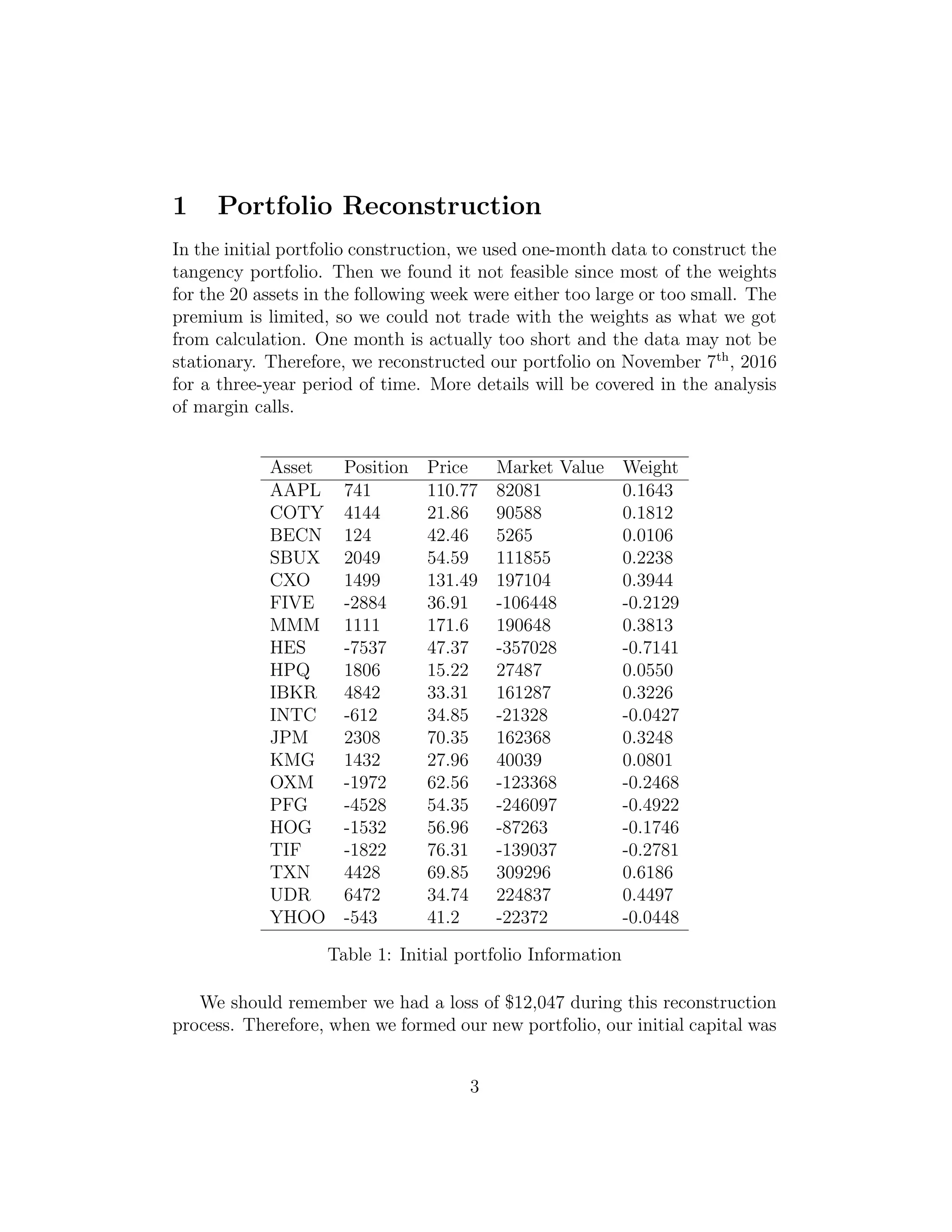
5. $987,953. The basic information is stored in the table.
We closed all Interactive Brokers portfolio positions on Thursday Decem-
ber 8th, then analyze the overall portfolio performance with all the data we
gathered. We had 30 trading days in total, and we adjusted the portfolio 5
times.
2 Portfolio Performance
2.1 Portfolio value
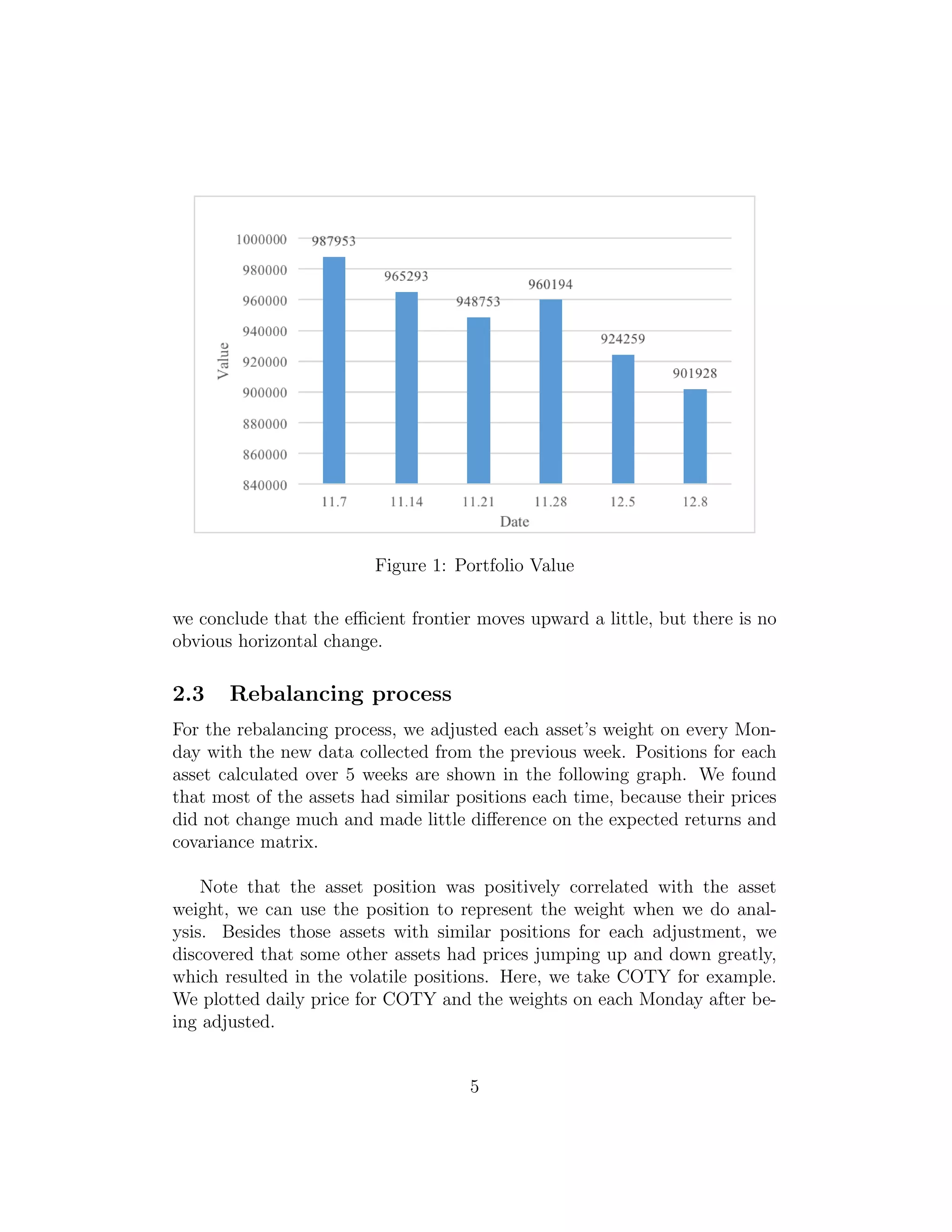
We plotted a histogram of weekly portfolio returns to track its performance,
and unfortunately, we had a loss of $86,025 ($987,953-$901,928) at last. We
presented all the portfolio values in the table and plot the distributions in
the histogram, from which we concluded that our investment failed to earn
profits.
Date 11.7 11.14 11.21 11.28 12.5 12.8
Portfolio Value 987,953 965,293 948,753 960,194 924,259 901,928
Table 2: Portfolio Value
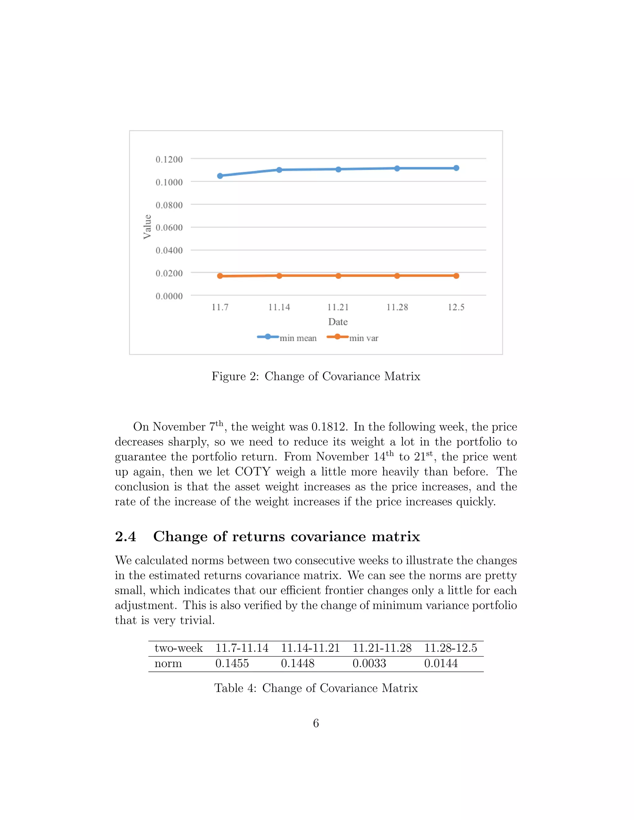
2.2 Efficient frontier (Minimum variance portfolio)
We can compare week-to-week minimum variance portfolios to illustrate how
the efficient frontier[1]
changes. The table and plot about minimum mean and
minimum variance are as follows:
Date 11.7 11.14 11.21 11.28 12.5
min mean 0.1050 0.1101 0.1106 0.1114 0.1117
min variance 0.0170 0.0172 0.0172 0.0171 0.0171
Table 3: Change of Efficient Frontier
Through our adjustments, the minimum variance oscillates between the
interval [0.0170, 0.0172] and the minimum mean slightly increases. Therefore,
4

6. Figure 1: Portfolio Value
we conclude that the efficient frontier moves upward a little, but there is no
obvious horizontal change.
2.3 Rebalancing process
For the rebalancing process, we adjusted each asset’s weight on every Mon-
day with the new data collected from the previous week. Positions for each
asset calculated over 5 weeks are shown in the following graph. We found
that most of the assets had similar positions each time, because their prices
did not change much and made little difference on the expected returns and
covariance matrix.
Note that the asset position was positively correlated with the asset
weight, we can use the position to represent the weight when we do anal-
ysis. Besides those assets with similar positions for each adjustment, we
discovered that some other assets had prices jumping up and down greatly,
which resulted in the volatile positions. Here, we take COTY for example.
We plotted daily price for COTY and the weights on each Monday after be-
ing adjusted.
5

7. Figure 2: Change of Covariance Matrix
On November 7th
, the weight was 0.1812. In the following week, the price
decreases sharply, so we need to reduce its weight a lot in the portfolio to
guarantee the portfolio return. From November 14th
to 21st
, the price went
up again, then we let COTY weigh a little more heavily than before. The
conclusion is that the asset weight increases as the price increases, and the
rate of the increase of the weight increases if the price increases quickly.
2.4 Change of returns covariance matrix
We calculated norms between two consecutive weeks to illustrate the changes
in the estimated returns covariance matrix. We can see the norms are pretty
small, which indicates that our efficient frontier changes only a little for each
adjustment. This is also verified by the change of minimum variance portfolio
that is very trivial.
two-week 11.7-11.14 11.14-11.21 11.21-11.28 11.28-12.5
norm 0.1455 0.1448 0.0033 0.0144
Table 4: Change of Covariance Matrix
6

8. Figure 3: Rebalance Process
2.5 Overall performance
For the overall portfolio performance, our initial portfolio value was $987,953,
and the ending value was $901,928. Therefore, we lost $86,025 in total.
Unfortunately, our portfolio was a failure.
3 Portfolio Performance Analysis
We collected all the daily prices[2]
for the 20 assets in our portfolio from
November 7th
to December 7th
, and would use this sample to do the follow-
ing portfolio performance analysis.
3.1 Sharpe ratio
The Sharpe ratio of a portfolio is its excess returns per unit of total portfolio
risk, and higher Sharpe ratios indicate better risk-adjusted portfolio perfor-
mance. The formula for Sharpe ratio is RS =
µp−µf
σp
. Here, we used sample
7

9. Figure 4: COTY Price
Figure 5: COTY Weight
8

10. mean return for µp and sample standard deviation of returns for σp. Also
for µf , we selected 12-month LIBOR[3]
as the risk-free rate which is 1.57%.
Finally we got Sharpe ratio is -0.370. Therefore, the return decreases 0.37
units for every unit of total risk.
3.2 Treynor ratio
The Treynor ratio is interpreted as excess returns per unit of systematic risk,
and is calculated as
µp−µf
βp
. We used S&P 500 as benchmark. The final result
was 0.072. In theory, the higher the Treynor ratio, the better the portfolio
performance. But we think the prerequisite should be: βp is positive. Indeed,
βp for our portfolio is negative, and µp is smaller than µf which is also not
ideal. Under this circumstance, we got a positive Treynor ratio. Therefore,
we cannot conclude that the portfolio is managed well.
3.3 Information ratio
Information ratio measures the average of an active portfolio return in excess
of a positive portfolio return. It is relative to the increased volatility of active
portfolio compared to the passive one. The formula to calculate Information
ratio is RI =
µp−µf
σRp−RM
, and S&P 500[4]
is used as benchmark here. The
information ratio for our portfolio is -0.016.
3.4 Sortino ratio
The Sortino ratio is calculated as µp−r0
σr−
0
. It is similar to Sharpe ratio, but
penalize only those returns falling below a required rate of return. r0 is
either a target return or some minimal acceptable return, often r0 = µf , σr−
0
is the left simivariance, defined as
ro
− inf
r0(x − r0)2
f(x)dx. But we can use
S2
a− which is calculated as 1
n
n
i=1[min{0, Ri − a}]2
to estimate σr−
0
. We set
a = 0, this means we only involve those negative portfolio returns in the
denominator. The Sortino ratio calculated is -0.017.
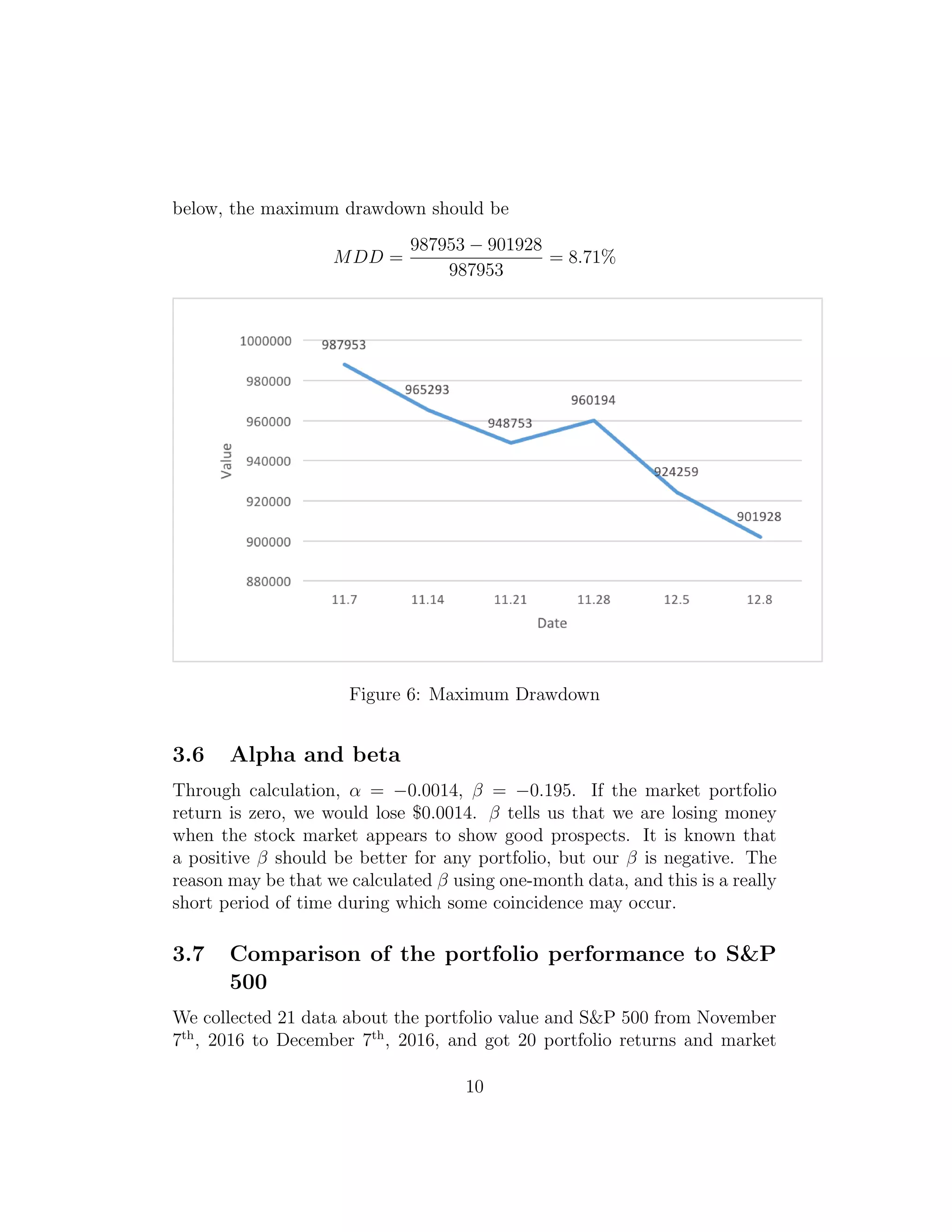
3.5 Maximum drawdown
Maximum drawdown is the maximal equity retracement of a portfolio over
some fixed period of time. Based on our week-to-week portfolio values shown
9

11. below, the maximum drawdown should be
MDD =
987953 − 901928
987953
= 8.71%
Figure 6: Maximum Drawdown
3.6 Alpha and beta
Through calculation, α = −0.0014, β = −0.195. If the market portfolio
return is zero, we would lose $0.0014. β tells us that we are losing money
when the stock market appears to show good prospects. It is known that
a positive β should be better for any portfolio, but our β is negative. The
reason may be that we calculated β using one-month data, and this is a really
short period of time during which some coincidence may occur.
3.7 Comparison of the portfolio performance to S&P
500
We collected 21 data about the portfolio value and S&P 500 from November
7th
, 2016 to December 7th
, 2016, and got 20 portfolio returns and market
10

12. returns respectively. We plotted these two returns below, and found that the
S&P 500 return was very stationary while our portfolio return jumped up
and down. S&P 500 is an American stock market index based on the market
capitalizations of 500 large companies[5]
. Indeed we selected a few small-cap
stocks in our portfolio, so the fluctuations seemed rational.
Figure 7: Portfolio vs Market
3.8 Margin calls
We failed to construct our initial portfolio at the first attempt. Because
when we tried to adjust the tangency portfolio in the following week, we
found many weights were either too high or too low, and we could not trade
based on these weights since our capital and premium were limited. If not,
the excess liquidity would fall below zero and we would be in margin viola-
tion. Then we realized the source of mistake should be the one-month data.
Since one month is really short, we cannot consider the asset prices are sta-
tionary and consistent. We need to choose another long period of time like
three years as we did at last.
11

13. After this adjustment of time series, the tangency portfolio weights ap-
peared reasonable over the following five weeks. The excess liquidity was
always positive in the remaining time, and we were never in margin violation
again.
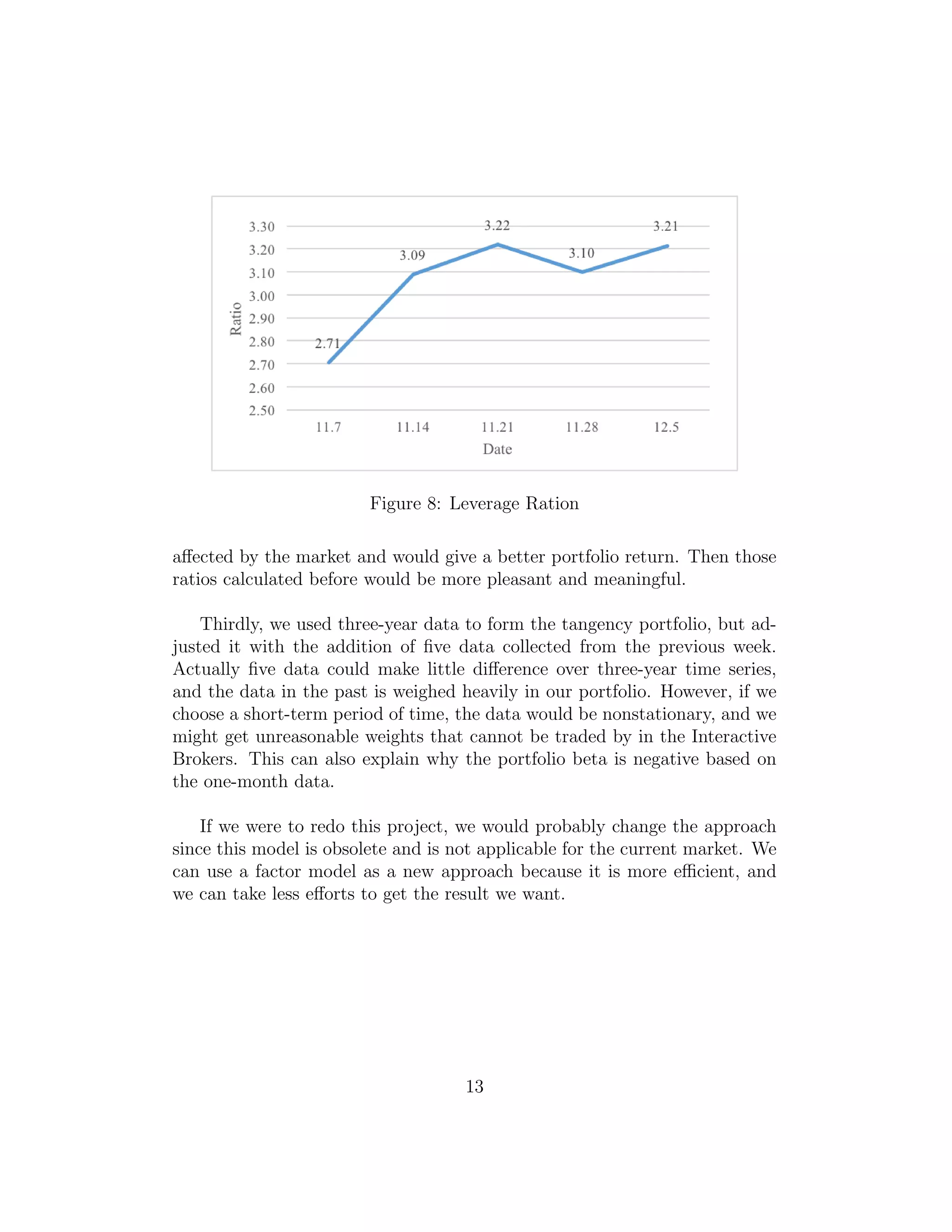
4 Leverage Analysis
The leverage is the use of various financial instruments or borrowed capi-
tal to increase the potential return of an investment, and is calculated as
|marketvalue|
$987,953
. High leverage ratios will bring high risks in the portfolio invest-
ment. We plot the leverage ratios below, and found that the leverage ratio
increases in general. Given that we had a loss of $86025 when we closed all
positions, we can assume such a scenario may exist: the price of one asset
increased in the last week, then we should buy more shares of it on the next
Monday, but the stock price begins to decrease after we enlarge its weight.
We certainly lose money in this scenario, and probably lose more with a high
leverage ratio. In addition, the fact that an asset has an increasing price
after we sell it will also reduce the portfolio value.
Date 11.7 11.14 11.21 11.28 12.5
Leverage Ratio 2.71 3.09 3.22 3.10 3.21
Table 5: Leverage Ratio
5 Conclusions
For this portfolio management, our critical mistake is that we chose a too
short period of time and ignored the margin violation at the beginning, so
we had to reconstruct a new portfolio and could not avoid losing some wealth.
Secondly, some of our stocks are highly correlated, such as AAPL and
HPQ (electronic products), or JPM and IBKR (finance). Our portfolios may
not be diversified greatly while diversification can reduce the unsystematic
risk[6]
which is a component of total risk together with systematic risk. If our
portfolio involves as many fields as possible, the portfolio may not be easily
12

14. Figure 8: Leverage Ration
affected by the market and would give a better portfolio return. Then those
ratios calculated before would be more pleasant and meaningful.
Thirdly, we used three-year data to form the tangency portfolio, but ad-
justed it with the addition of five data collected from the previous week.
Actually five data could make little difference over three-year time series,
and the data in the past is weighed heavily in our portfolio. However, if we
choose a short-term period of time, the data would be nonstationary, and we
might get unreasonable weights that cannot be traded by in the Interactive
Brokers. This can also explain why the portfolio beta is negative based on
the one-month data.
If we were to redo this project, we would probably change the approach
since this model is obsolete and is not applicable for the current market. We
can use a factor model as a new approach because it is more efficient, and
we can take less efforts to get the result we want.
13

15. 6 Factor Modeling
6.1 Fit the returns distribution to both a normal and
a t density
In our factor modeling project, the two factors we chose are 10-year bond
yield and big value[7]
. Through calculation, we found that CAPM with both
two factors and the French and Fama model with both two factors worked
well, also CAPM was better than French and Fama model in that case.
Therefore, we select CAPM with those two factors here.
For the new model, we constructed the new portfolio. Based on the stock
data, we can compute the portfolio daily return from January 1st
, 2016 to
October 31st
, 2016. The next step is to find a better distribution to fit the
return. We chose the normal distribution and the student-t distribution.
Based on the maximum of the likelihood function, our fitted parameters
are as below.
µ σ ν
Normal Distribution -0.0202489 0.165538 NaN
Student-t Distribution -0.0176197 0.150507 12.1176
Table 6: Parameter for Fitted Data
6.2 Perform a goodness-of-fit hypothesis test
For each of the distribution, based on the parameter before, we measured
the goodness of fit with the Chi-square test statistic. The null hypothesis is
to accept the fitted distribution.
p Decision
Normal Distribution 0.3115 Accept
Student-t Distribution 0.1290 Accept
Table 7: Decision for Hypothesis Test
Under the confidence level of α = 0.05, these two distribution can be
accepted to simulate the return of the portfolio.
14

16. References
[1] David Ruppert(2004), Statistics and Finance:An Introduction
[2] Yahoo Finance. Yahoo Finance Historical Prices.
Retrieved from: https://finance.yahoo.com/
[3] Federal Reserve Bank of St.Louis 3-Month London Interbank Offered
Rate, based on U.S. Dollar.
Retrieved from: https://fred.stlouisfed.org/
[4] Bloomberg. Bloomberg Terminal SPX Index.
[5] Investopedia. S&P 500 Index Definition.
Retrieved from: http://www.investopedia.com/terms
[6] Kaplan(2016). Unsystematic risk CFA level 1 schweser notes.
[7] Kenneth R. French. Big Value Data.
Retrieved from: http://mba.tuck.dartmouth.edu/pages/faculty/ken.french/
15

17. Appendices
16

18. 17