Spread spectrum Frequency-hopping spread spectrum (FHSS)

1. Spread Spectrum

2. Introduction to Spread Spectrum
• Problems such as capacity limits, propagation
effects, synchronization occur with wireless
systems
• Spread spectrum modulation spreads out the
modulated signal bandwidth so it is much
greater than the message bandwidth
• Independent code spreads signal at transmitter
and despreads signal at receiver

3. • Multiplexing in 4 dimensions
– space (si)
– time (t)
– frequency (f)
– code (c)
• Goal: multiple use
of a shared medium
• Important: guard spaces needed!
s2
s3
s1
Multiplexing
f
t
c
k2 k3 k4 k5 k6
k1
f
t
c
f
t
c
channels ki

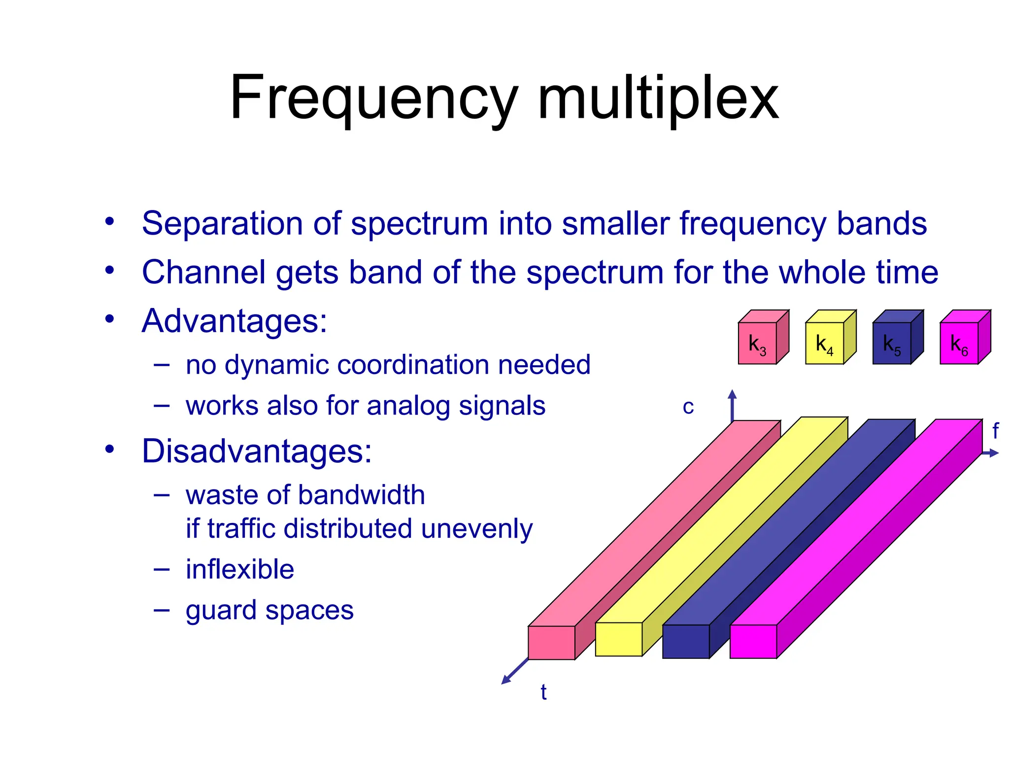
4. • Separation of spectrum into smaller frequency bands
• Channel gets band of the spectrum for the whole time
• Advantages:
– no dynamic coordination needed
– works also for analog signals
• Disadvantages:
– waste of bandwidth
if traffic distributed unevenly
– inflexible
– guard spaces
Frequency multiplex
k3 k4 k5 k6
f
t
c

5. f
t
c
k2 k3 k4 k5 k6
k1
Time multiplex
• Channel gets the whole spectrum for a certain
amount of time
• Advantages:
– only one carrier in the
medium at any time
– throughput high even
for many users
• Disadvantages:
– precise
synchronization
necessary

6. f
Time and frequency multiplex
• A channel gets a certain frequency band for a
certain amount of time (e.g. GSM)
• Advantages:
– better protection against tapping
– protection against frequency
selective interference
– higher data rates compared to
code multiplex
• Precise coordination
required
t
c
k2 k3 k4 k5 k6
k1

7. Code multiplex
• Each channel has unique code
• All channels use same spectrum at same time
• Advantages:
– bandwidth efficient
– no coordination and synchronization
– good protection against interference
• Disadvantages:
– lower user data rates
– more complex signal regeneration
• Implemented using spread spectrum technology
k2 k3 k4 k5 k6
k1
f
t
c

8. Spread Spectrum Technology
• Problem of radio transmission: frequency dependent
fading can wipe out narrow band signals for duration
of the interference
• Solution: spread the narrow band signal into a broad
band signal using a special code
detection at
receiver
interference
spread
signal
signal
spread
interference
f f
power
power

9. Spread Spectrum Technology
• Side effects:
– coexistence of several signals without dynamic
coordination
– tap-proof
• Alternatives: Direct Sequence (DS/SS), Frequency
Hopping (FH/SS)
• Spread spectrum increases BW of message signal
by a factor N, Processing Gain
10
Processing Gain 10log
ss ss
B B
N
B B
 
   
 

10. Effects of spreading and
interference
P
f
i)
P
f
ii)
sender
P
f
iii)
P
f
iv)
receiver
f
v)
user signal
broadband interference
narrowband interference
P

11. Spreading and frequency
selective fading
frequency
channel
quality
1 2
3
4
5 6
Narrowband
signal
guard space
2
2
2
2
2
frequency
channel
quality
1
spread
spectrum
narrowband
channels
spread spectrum
channels

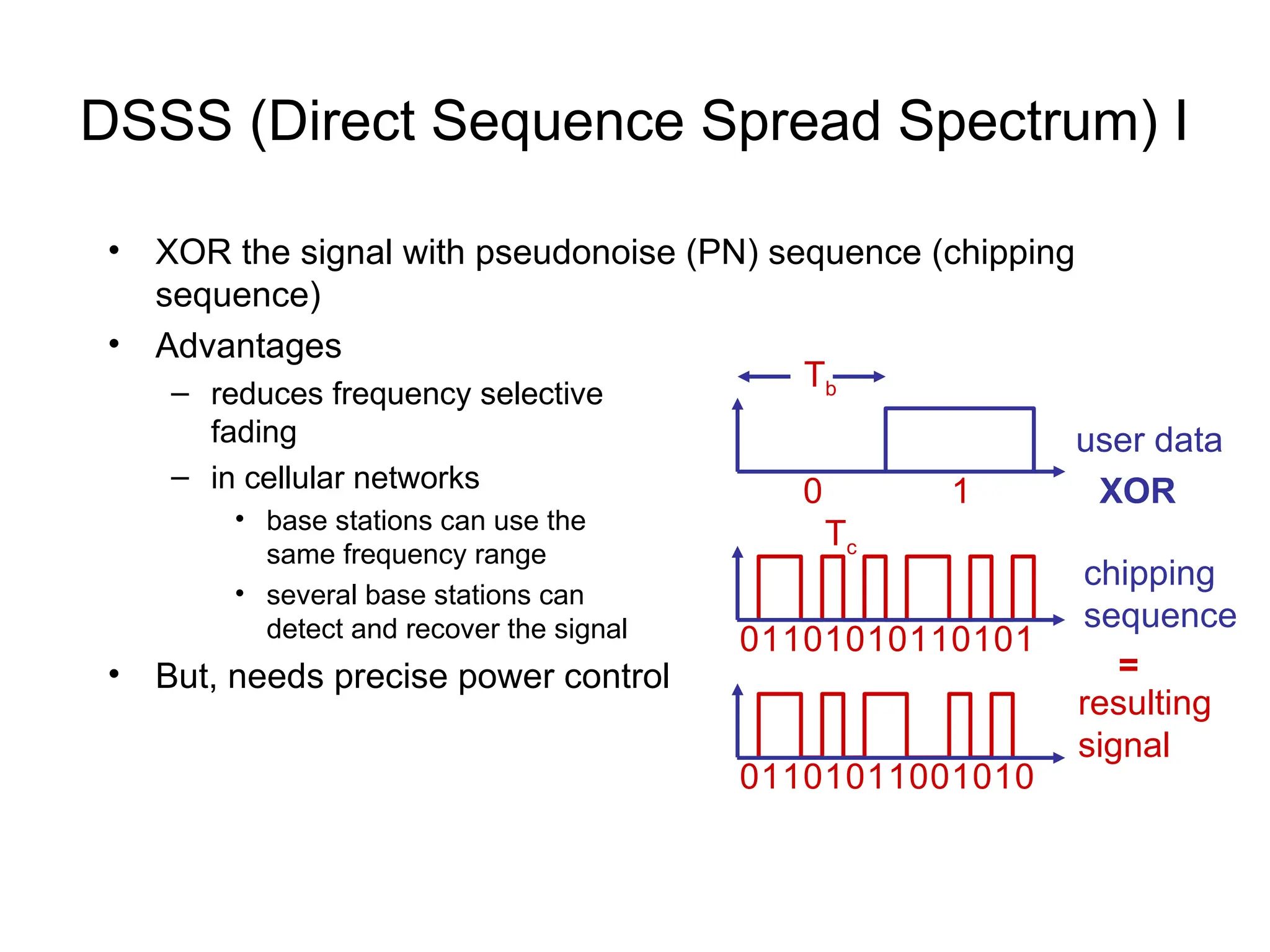
12. DSSS (Direct Sequence Spread Spectrum) I
• XOR the signal with pseudonoise (PN) sequence (chipping
sequence)
• Advantages
– reduces frequency selective
fading
– in cellular networks
• base stations can use the
same frequency range
• several base stations can
detect and recover the signal
• But, needs precise power control
user data
chipping
sequence
resulting
signal
0 1
0 1 10 1 010
1 0 0 1 1
1
XOR
0 1 10 0 101
1 0 1 0 0
1
=
Tb
Tc

13. user data
m(t)
chipping
sequence, c(t)
X
DSSS (Direct Sequence Spread Spectrum) II
modulator
radio
carrier
Spread spectrum
Signal y(t)=m(t)c(t) transmit
signal
transmitter
demodulator
received
signal
radio
carrier
X
Chipping sequence,
c(t)
receiver
integrator
products
decision
data
sampled
sums
correlator

14. DS/SS Comments III
• Pseudonoise(PN) sequence chosen so
that its autocorrelation is very narrow =>
PSD is very wide
– Concentrated around < Tc
– Cross-correlation between two user’s codes is
very small

15. DS/SS Comments IV
• Secure and Jamming Resistant
– Both receiver and transmitter must know c(t)
– Since PSD is low, hard to tell if signal present
– Since wide response, tough to jam everything
• Multiple access
– If ci(t) is orthogonal to cj(t), then users do not interfere
• Near/Far problem
– Users must be received with the same power

16. FH/SS (Frequency Hopping
Spread Spectrum) I
• Discrete changes of carrier frequency
– sequence of frequency changes determined via PN sequence
• Two versions
– Fast Hopping: several frequencies per user bit (FFH)
– Slow Hopping: several user bits per frequency (SFH)
• Advantages
– frequency selective fading and interference limited to short period
– uses only small portion of spectrum at any time
• Disadvantages
– not as robust as DS/SS
– simpler to detect

17. FHSS (Frequency Hopping
Spread Spectrum) II
user data
slow
hopping
(3 bits/hop)
fast
hopping
(3 hops/bit)
0 1
Tb
0 1 1 t
f
f1
f2
f3
t
Td
f
f1
f2
f3
t
Td
Tb: bit period Td: dwell time

18. FHSS (Frequency Hopping Spread Spectrum) III
modulator
user data
hopping
sequence
modulator
narrowband
signal
Spread transmit
signal
transmitter
received
signal
receiver
demodulator
data
frequency
synthesizer
hopping
sequence
demodulator
frequency
synthesizer

19. Applications of Spread
Spectrum
• Cell phones
– IS-95 (DS/SS)
– GSM
• Global Positioning System (GPS)
• Wireless LANs
– 802.11b

20. Performance of DS/SS Systems
• Pseudonoise (PN) codes
– Spread signal at the transmitter
– Despread signal at the receiver
• Ideal PN sequences should be
– Orthogonal (no interference)
– Random (security)
– Autocorrelation similar to white noise (high at
=0 and low for  not equal 0)

21. PN Sequence Generation
• Codes are periodic and generated by a shift register and XOR
• Maximum-length (ML) shift register sequences, m-stage shift
register, length: n = 2m
– 1 bits
R()
-1/n Tc

-nTc
nTc
+
Output

22. Generating PN Sequences
• Take m=2 =>L=3
• cn=[1,1,0,1,1,0, . . .],
usually written as
bipolar cn=[1,1,-1,1,1,-1,
. . .]
m Stages connected
to modulo-2 adder
2 1,2
3 1,3
4 1,4
5 1,4
6 1,6
8 1,5,6,7
+
Output
 









 


1
1
/
1
0
1
1
1
L
m
L
m
c
c
L
m
R
L
n
m
n
n
c

23. Problems with m-sequences
• Cross-correlations with other m-
sequences generated by different input
sequences can be quite high
• Easy to guess connection setup in 2m
samples so not too secure
• In practice, Gold codes or Kasami
sequences which combine the output of
m-sequences are used.

24. Detecting DS/SS PSK Signals
X
Bipolar, NRZ
m(t)
PN
sequence, c(t)
X
sqrt(2)cos(ct + )
Spread spectrum
Signal y(t)=m(t)c(t) transmit
signal
transmitter
X
received
signal
X
c(t)
receiver
integrator
z(t)
decision
data
sqrt(2)cos(ct + )
LPF
w(t)
x(t)

25. Optimum Detection of DS/SS PSK
• Recall, bipolar signaling (PSK) and white noise
give the optimum error probability
• Not effected by spreading
– Wideband noise not affected by spreading
– Narrowband noise reduced by spreading
2 b
b
E
P Q
 
  
 

 

26. Signal Spectra
• Effective noise power is channel noise power
plus jamming (NB) signal power divided by N
10
Processing Gain 10log
ss ss b
c
B B T
N
B B T
 
  
 
 
Tb
Tc

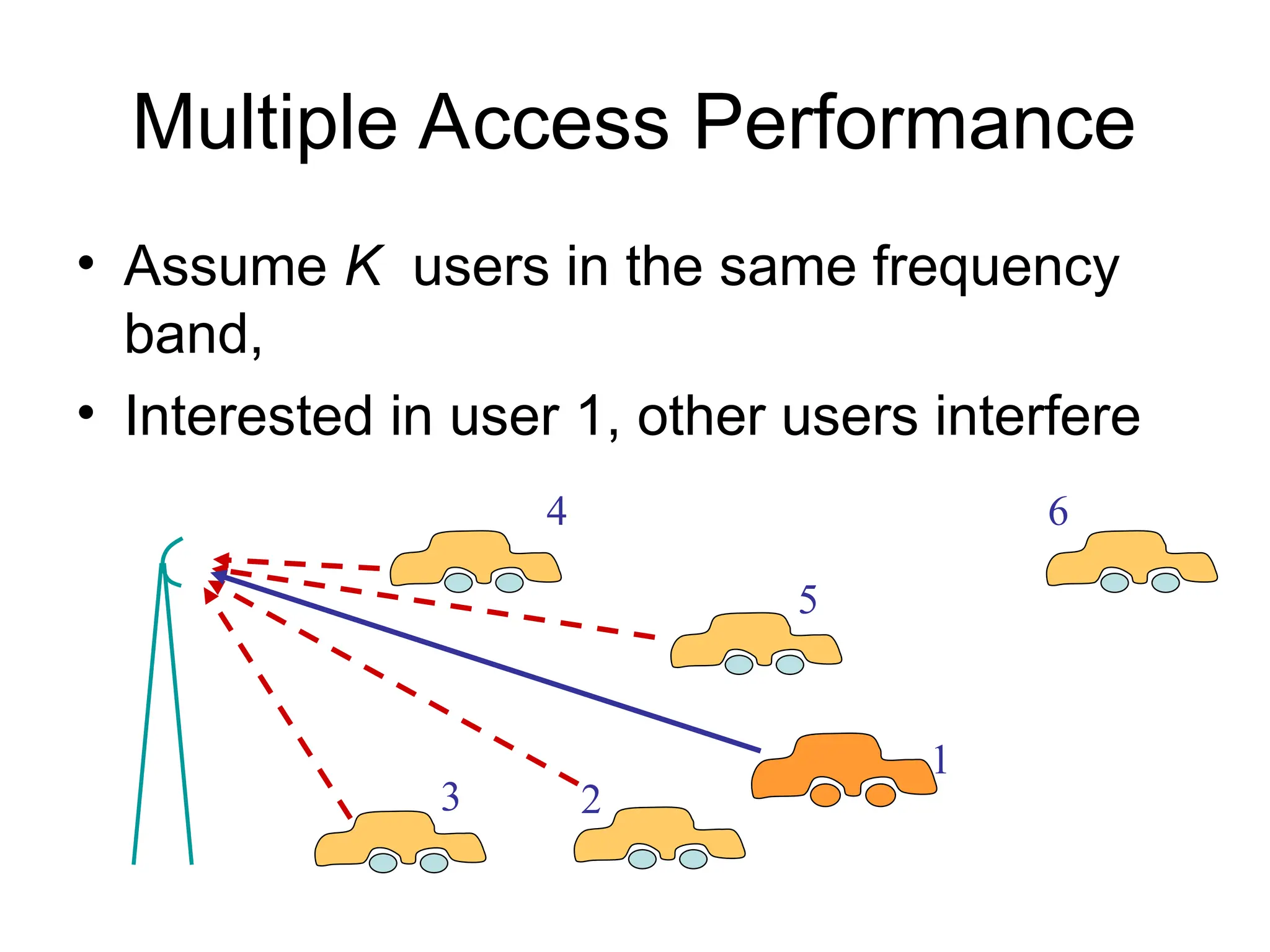
27. Multiple Access Performance
• Assume K users in the same frequency
band,
• Interested in user 1, other users interfere
4
1
3
5
2
6

28. Signal Model
• Interested in signal 1, but we also get
signals from other K-1 users:
• At receiver,
       
 
     
2 cos
2 cos
k k k k k c k k
k k k k c k k k c k
x t m t c t t
m t c t t
    
       
    
     
     
1
2
K
k
k
x t x t x t

  

29. Interfering Signal
• After mixing and despreading (assume 1=0)
• After LPF
• After the integrator-sampler
           
1 1
2 cos cos
k k k k k c k c
z t m t c t c t t t
     
    
         
1 1
cos
k k k k k k
w t m t c t c t
   
   
       
1 1
0
cos b
T
k k k k k k
I m t c t c t dt
   
   


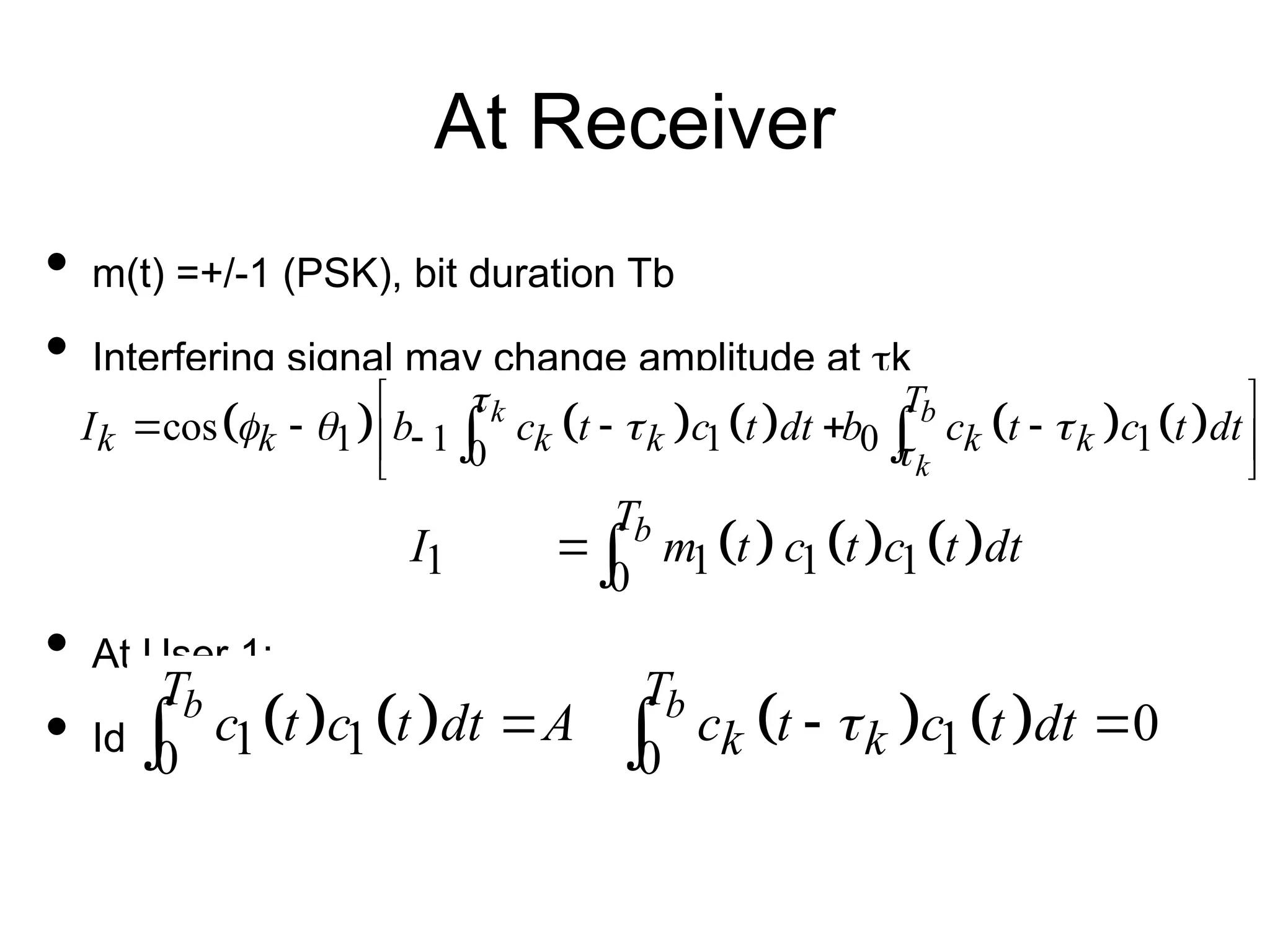
30. At Receiver
• m(t) =+/-1 (PSK), bit duration Tb
• Interfering signal may change amplitude at k
• At User 1:
• Ideally, spreading codes are Orthogonal:
         
1 1 1 0 1
0
cos k b
k
T
k k k k k k
I b c t c t dt b c t c t dt


   

 
    
 
 
 
     
1 1 1 1
0
b
T
I m t c t c t dt

       
1 1 1
0 0
0
b b
T T
k k
c t c t dt A c t c t dt

  
 

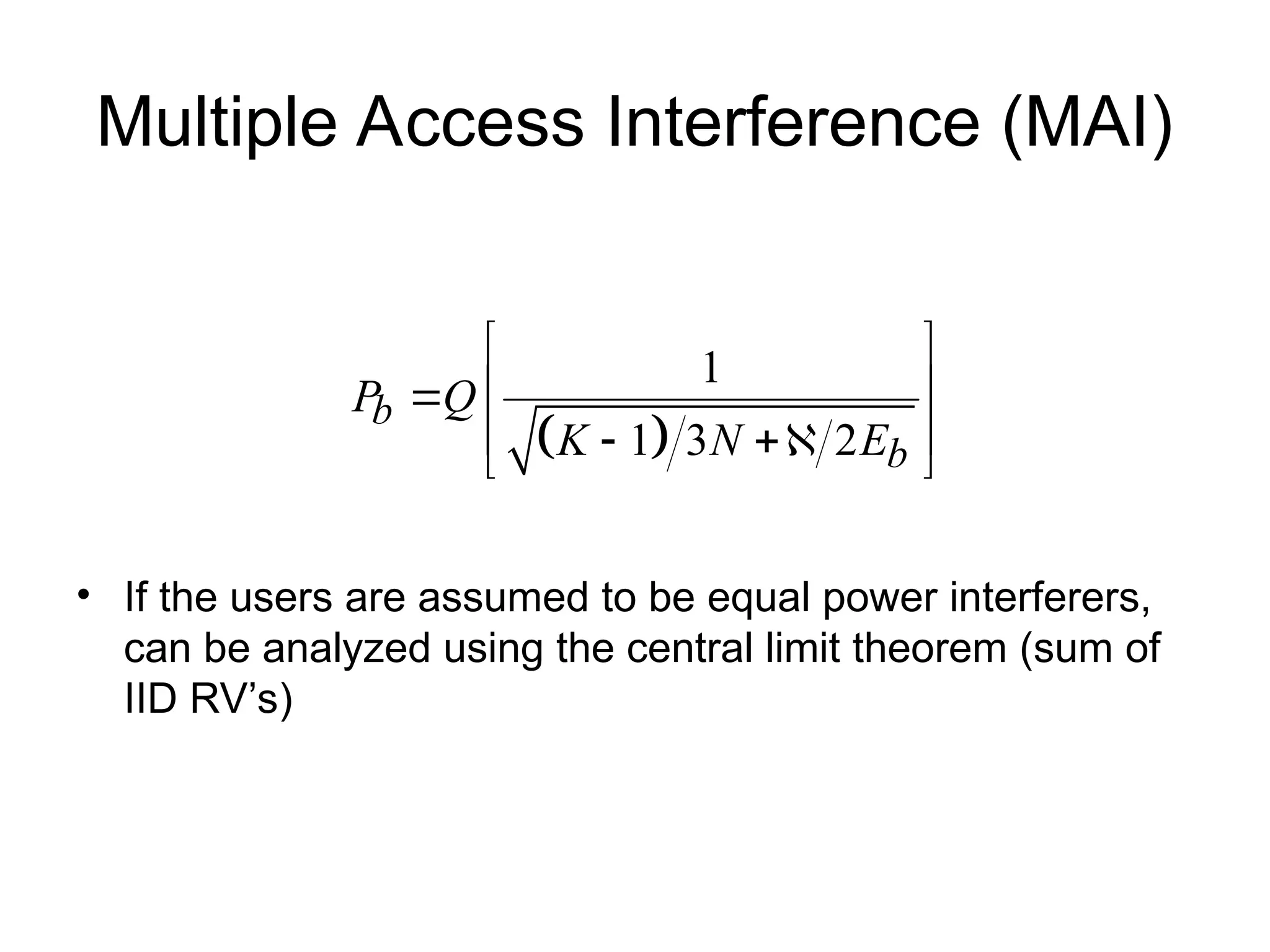
31. Multiple Access Interference (MAI)
• If the users are assumed to be equal power interferers,
can be analyzed using the central limit theorem (sum of
IID RV’s)
 
1
1 3 2
b
b
P Q
K N E
 
 

 
 
 

32. Example of Performance
Degradation
N=8 N=32

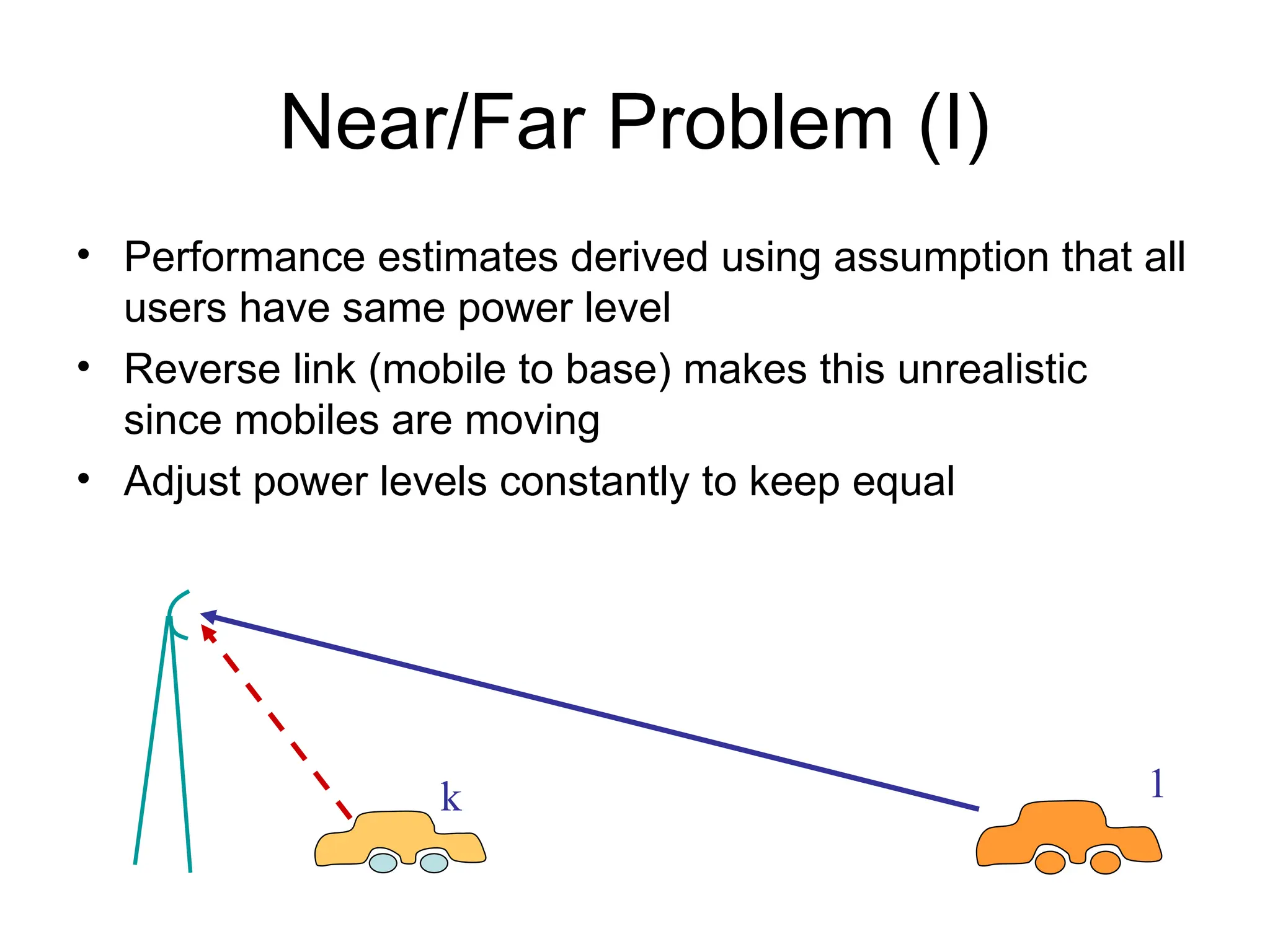
33. Near/Far Problem (I)
• Performance estimates derived using assumption that all
users have same power level
• Reverse link (mobile to base) makes this unrealistic
since mobiles are moving
• Adjust power levels constantly to keep equal
1
k

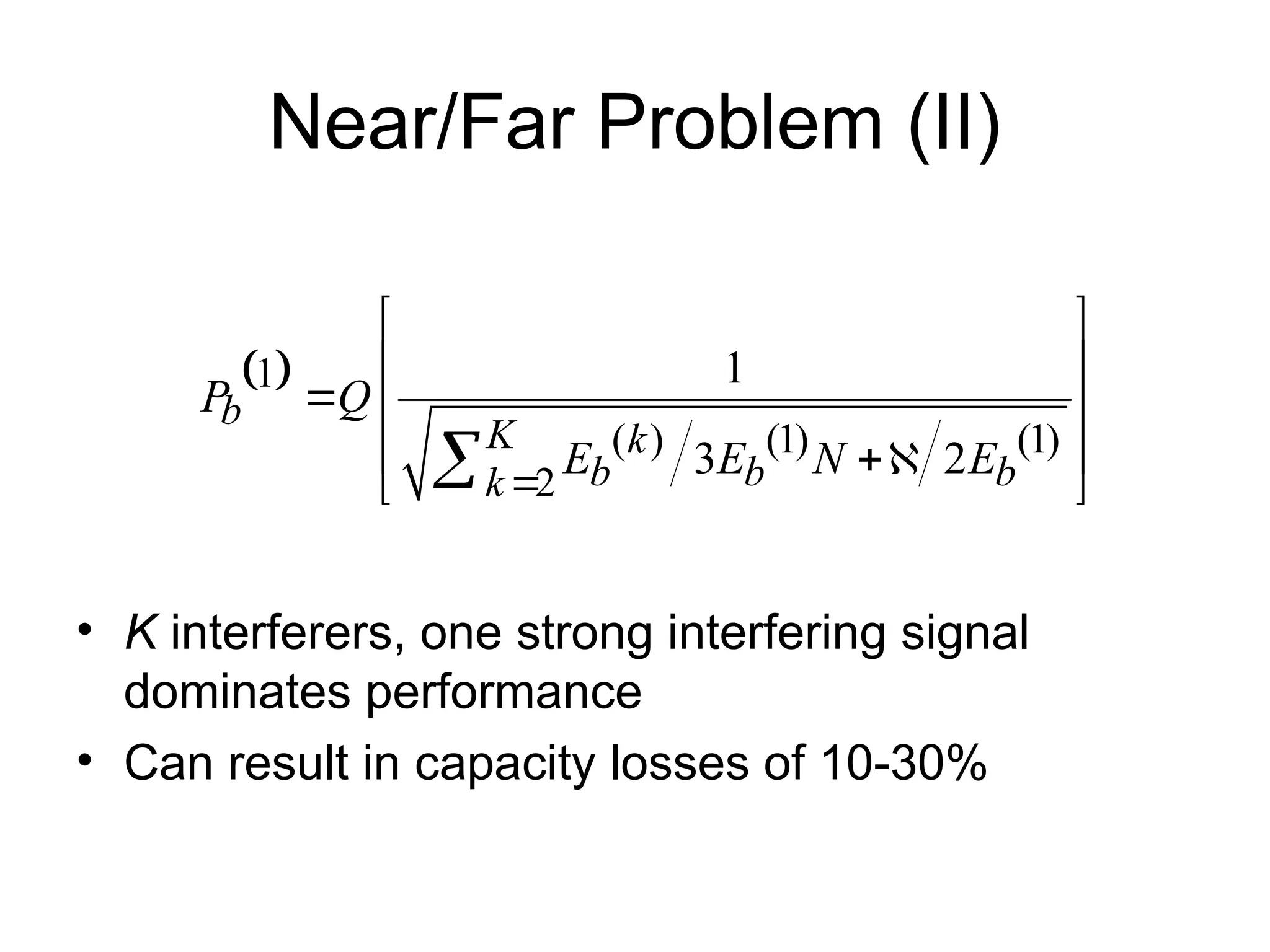
34. Near/Far Problem (II)
• K interferers, one strong interfering signal
dominates performance
• Can result in capacity losses of 10-30%
 
1
( ) (1) (1)
2
1
3 2
b
K k
b b b
k
P Q
E E N E

 
 
  
 

 


35. Multipath Propagation

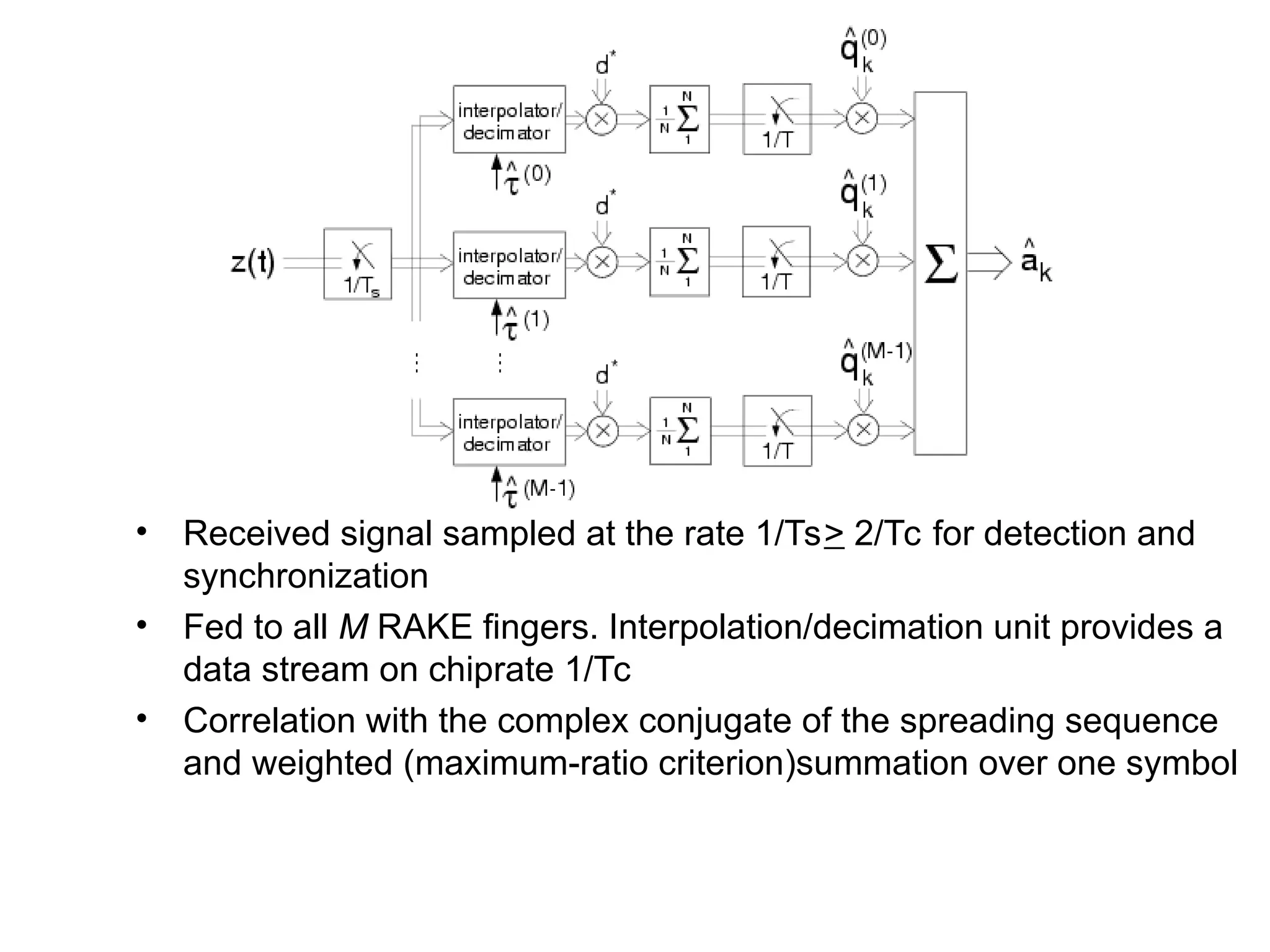
36. RAKE Receiver
• Received signal sampled at the rate 1/Ts> 2/Tc for detection and
synchronization
• Fed to all M RAKE fingers. Interpolation/decimation unit provides a
data stream on chiprate 1/Tc
• Correlation with the complex conjugate of the spreading sequence
and weighted (maximum-ratio criterion)summation over one symbol

37. RAKE Receiver
• RAKE Receiver has to estimate:
– Multipath delays
– Phase of multipath components
– Amplitude of multipath components
– Number of multipath components
• Main challenge is receiver synchronization in
fading channels