Spherical Harmonics.pdf

Spherical Harmonics 1
Spherical Harmonics
목차
1. 개요
2. Irradiance Map
3. 버금르장드르다항식(Associated Legendre Polynomials)
4. 구면조화함수
5. 투영(Projection)
6. 구면조화함수를이용한Irradiance Map
7. 마치며
8. Reference
개요
Spherical Harmonics(이하구면조화함수)는구면좌표계에서정의되는함수입니다. 구면조화함수에대한위키페이지를
보면다음과같이구면조화함수를설명하고있습니다.
수학과물리학에서구면조화함수(球面調和函數, 영어: spherical harmonics)는구면에서라플
라스방정식의해의정규직교기저다. 전자기학과양자역학등에서구면대칭인계를다룰때쓰
인다.
참난해한설명입니다. 하지만다행스럽게도구면조화함수의몇몇특징을이해한다면렌더링영역에서구면조화함수를도
구로사용할수있습니다.
여기서는Irradiance Map을 Direct3D 11/12로구현한결과물을통해구면조화함수의몇가지특징에대해살펴보도록하
겠습니다.
Irradiance Map
Irradiance Map은이미지를광원으로하는Image Based Lighting(이하IBL)의일종입니다. 이중에서Diffuse 반사를위해
사전에필터링한이미지를Irradiance Map이라합니다. 다음과같이대체로360도전방향을포함할수있는큐브맵을사용
합니다.
출처: https://learnopengl.com/PBR/IBL/Diffuse-irradiance

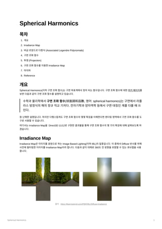
Irradiance Map은360도전방향에대하여다음과같은렌더링방정식을계산하는것으로생성할수있습니다.
: 반사되는radiance
: 반사표면
: 빛이나가는방향, 빛이들어오는방향
: 표면에서방출되는radiance
: 반구공간
: brdf
: 입사되는radiance
Diffuse 반사에서brdf는대체로Lambert BRDF가사용되며Lambert BRDF는상수이기때문에brdf를적분의밖으로빼낼
수있습니다. 또한반사표면에서방출되는빛이없다고한다면위식을아래와같이단순화할수있습니다.
여기서Lambert BRDF를제외하면Irradiance가됩니다.
이제실제코드로Irradiance Map을생성하는과정을살펴보겠습니다. 먼저구면조화함수를사용하지않는경우에어떻게
구현되는지보겠습니다. 여기서는원본큐브맵(2048x2048)보다작은큐브맵(32x32)으로위의식을일일이계산하여
Irradiance Map을생성합니다. 주파수가낮은Diffuse 반사의특징으로인해작은큐브맵을사용하여도텍스쳐보간이있기
때문에괜찮습니다.
먼저Irradiance Map을위한큐브맵을생성하는코드입니다.
agl::TextureTrait trait = cubeMap->GetTrait();
trait.m_width = trait.m_height = 32; // 원본 큐브맵에서 크기 변경
trait.m_format = agl::ResourceFormat::R8G8B8A8_UNORM_SRGB;
trait.m_bindType |= agl::ResourceBindType::RenderTarget; // 렌더 타겟으로 사용
auto irradianceMap = agl::Texture::Create( trait );
EnqueueRenderTask( [irradianceMap]()
{
irradianceMap->Init();
} );
이렇게생성된큐브맵을렌더타겟으로하고지오메트리셰이더를사용하여한번의드로우콜로모든면에대한Irradiance
Map을생성합니다. 버택스셰이더와지오메트리셰이더를차례대로보겠습니다.
버택스셰이더입니다. 실제정육면체메시는지오메트리셰이더에서생성할것이므로SV_VertexID를사용하여각면에대
한인덱스만을지오메트리셰이더로전달합니다. 따라서드로우콜의호출도버텍스버퍼와인덱스버퍼를바인딩하지않고
버택스수를6으로하여호출합니다.
struct VS_OUTPUT
{
uint vertexId : VERTEXID;
};
VS_OUTPUT main( uint vertexId : SV_VertexID )
{
VS_OUTPUT output = (VS_OUTPUT)0;
L
(x,ω
) = L
(x,ω
) + f
(x,ω
,ω )L
(x,ω
)(ω ⋅ n)d ω
r o e o ∫
Ω
r i o i i i i
L
(x,ω
)
r o
x
w
,w
o i
L
(x,ω
)
r o
Ω
f
(x,ω
,ω
)
r i o
L
(x,ω
)
i i
L
(x,ω
) =
L
(x,ω
)(ω
⋅ n)d ω
r o
π
σ
∫
Ω
i i i i
E(x) =
L
(x,ω
)(ω
⋅ n)d ω
∫
Ω
i i i i

output.vertexId = vertexId;
return output;
}
지오메트리셰이더입니다. 여기서정육면체메시에대한버택스를생성하여픽셀셰이더로전달합니다. 주목할부분은
GS_OUTPUT에SV_RenderTargetArrayIndex를사용했다는점입니다. 이것으로렌더링할큐브맵의면을지정할수있습
니다.
struct GS_INPUT
{
uint vertexId : VERTEXID;
};
struct GS_OUTPUT
{
float4 position : SV_POSITION;
float3 localPosition : POSITION0;
uint rtIndex : SV_RenderTargetArrayIndex;
};
static const float4 projectedPos[] =
{
{ -1, -1, 0, 1 },
{ -1, 1, 0, 1 },
{ 1, -1, 0, 1 },
{ 1, 1, 0, 1 }
};
static const float3 vertices[] =
{
{ -1, -1, -1 },
{ -1, 1, -1 },
{ 1, -1, -1 },
{ 1, 1, -1 },
{ -1, -1, 1 },
{ -1, 1, 1 },
{ 1, -1, 1 },
{ 1, 1, 1 }
};
static const int4 indices[] =
{
{ 6, 7, 2, 3 },
{ 0, 1, 4, 5 },
{ 5, 1, 7, 3 },
{ 0, 4, 2, 6 },
{ 4, 5, 6, 7 },
{ 2, 3, 0, 1 }
};
[maxvertexcount(4)]
void main( point GS_INPUT input[1], inout TriangleStream<GS_OUTPUT> triStream )
{
GS_OUTPUT output = (GS_OUTPUT)0;
output.rtIndex = input[0].vertexId;
for ( int i = 0; i < 4; ++i )
{
output.position = projectedPos[i];
int index = indices[input[0].vertexId][i];
output.localPosition = vertices[index];
triStream.Append( output );
}
triStream.RestartStrip();
}
픽셀셰이더를살펴보기전계산해야할식을정리할필요가있습니다.
표면에서반사되는radiance에대한식에서시작합니다.

Irrdiance를계산하고렌더링시Lambert BRDF를적용해도되지만Lambert BRDF가상수이기때문에여기서함께계산하
도록합니다. 여기서표면의알베도인
는렌더링시곱해주면되기때문에제외하여다음과같이정리할수있습니다.
이식을구면좌표계에대한적분으로다음과같이쓸수있습니다.
그리고픽셀셰이더에서계산할수있도록리만합을통해다음과같은형태로변경합니다.
이제픽셀셰이더를살펴보겠습니다.
#include "Common/Constants.fxh"
TextureCube CubeMap : register( t0 );
SamplerState LinearSampler : register( s0 );
static const float SampleDelta = 0.025f;
struct PS_INPUT
{
float4 position : SV_POSITION;
float3 localPosition : POSITION0;
uint rtIndex : SV_RenderTargetArrayIndex;
};
float4 main(PS_INPUT input) : SV_TARGET
{
float3 normal = normalize( input.localPosition );
float3 up = ( abs( normal.y ) < 0.999 ) ? float3( 0.f, 1.f, 0.f ) : float3( 0.f, 0.f, 1.f );
float3 right = normalize( cross( up, normal ) );
up = normalize( cross( normal, right ) );
float3x3 toWorld = float3x3( right, up, normal );
float3 irradiance = 0.f;
float numSample = 0.f;
for ( float phi = 0.f; phi < 2.f * PI; phi += SampleDelta )
{
for ( float theta = 0.f; theta < 0.5f * PI; theta += SampleDelta )
{
float3 tangentSample = float3( sin( theta ) * cos( phi ), sin( theta ) * sin( phi ), cos( theta ) );
float3 worldSample = normalize( mul( tangentSample, toWorld ) );
irradiance += CubeMap.Sample( LinearSampler, worldSample ).rgb * cos( theta ) * sin( theta );
++numSample;
}
}
irradiance = PI * irradiance / numSample;
L
(x,ω
) = L
(x,ω
)(ω ⋅ n)d ω
r o
π
σ
∫
Ω
i i i i
σ

L
(x,ω
)(ω ⋅
π
1
∫
Ω
i i i n)d ω
i
L(θ,ϕ)cos(θ)sin(θ)dθdϕ
π
1
∫
ϕ=0
2π
∫
θ=0

2
π
L
(x,ω
)cos(θ)sin(θ)
π
1
n1
2π
n2

2
π
ϕ=0
∑
n1
θ=0
∑
n2
i i
= L
(x,ω
)cos(θ)sin(θ)
n1n2
π
ϕ=0
∑
n1
θ=0
∑
n2
i i

return float4( irradiance, 1.f );
}
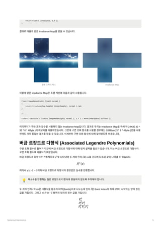
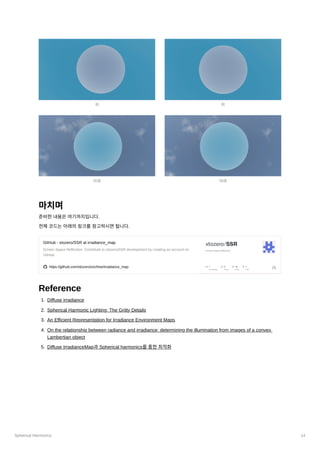
결과로다음과같은Irradiance Map을얻을수있습니다.
이렇게얻은Irradiance Map은조명계산에다음과같이사용됩니다.
float3 ImageBasedLight( float3 normal )
{
return IrradianceMap.Sample( LinearSampler, normal ).rgb;
}
// ...
float4 lightColor = float4( ImageBasedLight( normal ), 1.f ) * MoveLinearSpace( Diffuse );
여기까지가구면조화함수를사용하지않는Irradiance Map입니다. 결과로우리는Irradiance Map을위해약24KB( 32 *
32 * 6 * 4Byte )의메모리를사용하였습니다. 그런데구면조화함수를사용할경우에는108Byte( 3 * 9 * 4Byte )만을사용
하여도거의동일한결과를얻을수있습니다. 이제부터구면조화함수에대해알아보도록하겠습니다.
버금르장드르다항식(Associated Legendre Polynomials)
구면조화함수로들어가기전에버금르장드르다항식에대해먼저살펴볼필요가있습니다. 이는버금르장드르다항식이
구면조화함수에사용되기때문입니다.
버금르장드르다항식은전통적으로
로나타내며두개의인자
과
을가지며다음과같이나타낼수있습니다.
여기서
는-1 ~ 1이며버금르장드르다항식의결괏값은실수를반환합니다.
💡 복소수를반환하는일반르장드르다항식과혼동하지않도록주의해야합니다.
두개의인자
과
은다항식을함수의대역(Bands)으로나누는데인자
은Band Index라하여0부터시작하는양의정숫
값을가집니다. 그리고
은0 ~ 범위의임의의정수값을가집니다.
원본스카이박스 Irradiance Map
P l m
P
(x)
l
m
x
l m l
m l
P
0
0
P
P
1
0
1
1
P
P
P
2
0
2
1
2
2

버금르장드르다항식은여러가지재귀관계를가지고있는데이를통해모든다항식을계산할수있습니다. 여기서는3가지
식을소개하도록하겠습니다.
이식은이전결과와연관관계가없기때문에버금르장드르다항식을구하는시작점으로적합합니다. 여기서
는이중계승
을나타내는기호로다음과같이계산할수있습니다.
나머지두식은이전결과를이용합니다.

의값은1이기때문에이를초기상태로놓으면위의3가지식으로필요한버금르장드르다항식을구할수있습니다.
다음은3가지식을통해버금르장드르다항식의값을구하는코드입니다.
double P(int l, int m, double x)
{
// evaluate an Associated Legendre Polynomial P(l,m,x) at x
double pmm = 1.0;
if (m > 0)
{
double somx2 = sqrt((1.0 - x) * (1.0 + x))
double fact = 1.0;
for (int i = 1; i <= m; i++)
{
pmm *= (-fact) * somx2;
fact += 2.0;
}
}
if (l == m) return pmm;
double pmmp1 = x * (2.0 * m + 1.0) * pmm;
if (l == m + 1) return pmmp1;
double pll = 0.0;
for (int ll = m + 2; ll <= l; ++ll)
{
pll = ((2.0 * ll - 1.0) * x * pmmp1 - (ll + m - 1.0) * pmm) / (ll - m);
pmm = pmmp1;
pmmp1 = pll;
}
return pll;
}
구면조화함수
Spherical Harmonics를검색했을때나오는일반적인구면조화함수는다음과같습니다.
일반적인버금르장드르다항식과마찬가지로일반적인구면조화함수도복소수를반환하는데우리는실수에관심이있습니
다. 따라서여기서는실수구면조화함수에대해서알아볼것입니다.
실수구면조화함수는다음과같습니다.
1 P =
m
m
(−1) (2m −
m
1)!!(1 − x )
2 m/2
!!
n!! = {
n ⋅ (n − 2)...5 ⋅ 3 ⋅ 1, n > 0 odd
n ⋅ (n − 2)...6 ⋅ 4 ⋅ 2, n > 0 even
2 P =
m+1
m
x(2m + 1)P
m
m
3 (l − m)P
=
l
m
x(2l − 1)P
−
l−1
m
(l + m − 1)P
l−2
m
P
(x)
0
0
Y
(θ,ϕ) :=
l
m
AP
(cosθ)e
l
m imϕ

여기서
는앞에서살펴본버금르장드르다항식이며
는정규화를위한배율계수입니다.
모든구면조화함수에서
과
은버금르장드르다항식과조금다르게정의됩니다.
은여전히0에서시작하는양의정수이
지만
은
과
사이의정수입니다.
이를그래프로나타내면다음과같습니다.
위그래프는구면좌표계에서그려진구면조화함수의그래프로초록색은함수가양인구역붉은색은함수가음인구역을나
타냅니다.
다음은구면조화함수를구하는코드입니다.
double K(int l, int m)
{
// renormalisation constant for SH function
double temp = ((2.0 * l + 1.0) * factorial(l - m)) / (4.0 * PI * factorial(l + m));
return sqrt(temp);
}
double SH(int l, int m, double theta, double phi)
{
// return a point sample of a Spherical Harmonic basis function
// l is the band, range [0..N]
// m in the range [-l..l]
// theta in the range [0..Pi]
y
(θ,φ) =
l
m
{

K
cos(mφ)P
(cosθ), m > 0
2 l
m
l
m

K
sin(−mφ)P
(cosθ), m < 0
2 l
m
l
m
K
P
(cosθ), m = 0
l
0
l
0
P K
K =
l
m

4π
(2l + 1)
(l + ∣m∣)!
(l − ∣m∣)!
l m l
m −l l
y
0
0
y y y
1
−1
1
0
1
1
y y y y y
2
−2
2
−1
2
0
2
1
2
2
출처: https://users.soe.ucsc.edu/~pang/160/s13/projects/bgabin/Final/report/Spherical Harmonic Lighting Comparison.htm

// phi in the range [0..2*Pi]
const double sqrt2 = sqrt(2.0);
if (m == 0) return K(l, 0) * P(l, m, cos(theta));
else if (m > 0) return sqrt2 * K(l, m) * cos(m * phi) * P(l, m, cos(theta));
else return sqrt2 * K(l, -m) * sin(-m * phi) * P(l, -m, cos(theta));
}
버금르장드르다항식에팩토리얼까지구면조화함수를구하는과정은꽤복잡합니다. 하지만실제구현에서사용되는구면
조화함수는미리계산해놓은것이있기때문에매우간단하게구할수있습니다. 우선구면좌표계를익숙한데카르트좌표
계로다음과같이바꿀수있습니다.
그리고이를이용하여구면조화함수를다음과같이풀어사용할수있습니다. 다음은
까지의구면조화함수입니다.
투영(Projection)
이제우리는구면조화함수를구할수있습니다. 그럼본래의목적으로돌아와서어떻게하면Irradiance Map을구면조화
함수를이용하여최적화할수있을까요? 여기서기저함수(Basis Function)와투영(Projection)에대해살펴볼필요가있습
니다.
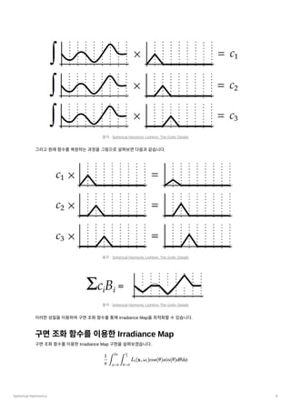
기저함수는선형조합을통해원래함수의근사치를생성할수있는함수입니다. 즉다음과같이기저함수에계수를곱하고
각각을더함으로써원래의함수를근사합니다.
기저함수에곱해질계수를구하는과정을투영이라고합니다. 투영을통해계수를얻기위해서는원본함수의전체영역에
걸쳐기저함수와의곱을적분하면됩니다.
투영과정을그림으로살펴보면다음과같습니다.
(x,y,z) = (sinθcosϕ,sinθsinϕ,cosθ)
l = 2
y
( ) =
0
0
n 0.282095
y
( ) =
1
−1
n 0.488603y
y
( ) =
1
0
n 0.488603z
y
( ) =
1
1
n 0.488603x
y
( ) =
2
−2
n 1.092548xy
y
( ) =
2
−1
n 1.092548yz
y
( ) =
2
0
n 0.315392(3z −
2
1)
y
( ) =
2
1
n 1.092548xz
y
( ) =
2
2
n 0.546274(x −
2
y )
2
f(x) = c
b
(x) +
1 1 c
b
(x) +
2 2 c
b
(x) +
3 3 c
b
(x) +
4 4 ...
c =
i f(x)b
(x)
∫ i

그리고원래함수를복원하는과정을그림으로살펴보면다음과같습니다.
이러한성질을이용하여구면조화함수를통해Irradiance Map을최적화할수있습니다.
구면조화함수를이용한Irradiance Map
구면조화함수를이용한Irradiance Map 구현을살펴보겠습니다.
출처: Spherical Harmonic Lighting: The Gritty Details
L
(x,ω
)cos(θ)sin(θ)dθdϕ
π
1
∫
ϕ=0
2π
∫
θ=0

2
π
i i

위수식을다음과같이2가지로나눕니다.
1. → 반구에대한적분에서구전체에대한적분으로변경되었습니다.
2. → 양수의범위로제한합니다. 구전체에대한Radiance의적분과곱해지면반구의반대편은0이되
어반구에대한Radiance만남게됩니다.
그리고투영을통해각각에대한구면조화함수의계수를구합니다.
여기서
는천정각(Zenith Angle)에만영향을받기때문에
은항상0이됩니다. 이렇게얻어낸계수 과
를통
해Irradiance를복원할수있습니다. Irradiance의구면조화함수계수를
이라할때Irradiance는다음과같이복원됩
니다.
이때
은
과
로다음과같이나타낼수있습니다.
여기서
은로컬좌표에서계산된
의구면조화함수계수를월드좌표로회전시키기위한가중치값입니다. 자
세한유도과정은레퍼런스4번의4.A에서설명하고있습니다.
편의를위해새로운변수
를다음과같이정의합니다.

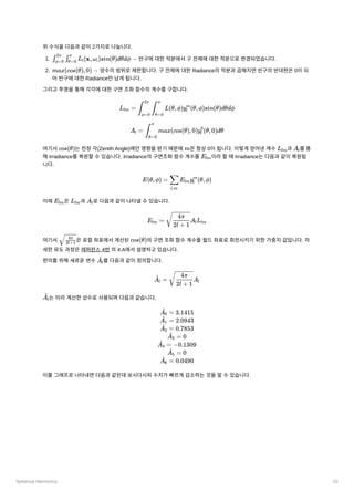
는미리계산한상수로사용되며다음과같습니다.
이를그래프로나타내면다음과같은데보시다시피수치가빠르게감소하는것을알수있습니다.
L
(x,ω
)sin(θ)dθdϕ
∫ϕ=0
2π
∫θ=0
π
i i
max(cos(θ),0)
L =
lm L(θ,ϕ)y
(θ,ϕ)sin(θ)dθdϕ
∫
ϕ=0
2π
∫
θ=0
π
l
m
A =
l max(cos(θ),0)y
(θ,0)dθ
∫
θ=0
π
l
0
cos(θ) m Llm A
l
E
lm
E(θ,ϕ) = E
y
(θ,ϕ)
l,m
∑ lm l
m
E
lm L
lm A
l
E
=
lm
A
L

2l + 1
4π
l lm

2l+1
4π
cos(θ)

A
l
^

=
A
l
^
A

2l + 1
4π
l

A
l
^
=
A
0
^ 3.1415
=
A
1
^ 2.0943
=
A
2
^ 0.7853
=
A
3
^ 0

=
A
4
^ −0.1309
=
A
5
^ 0

=
A
6
^ 0.0490

따라서
의낮은주파수의구면조화함수로도충분하기때문에27개의계수(RGB 색상3개* SH 계수9개)만으로
Irradiance Map을근사할수있습니다. 따라서셰이더코드에서구면조화함수
을구하는함수는다음과같이작성됩
니다.
void ShFunctionL2( float3 v, out float Y[9] )
{
// L0
Y[0] = 0.282095f; // Y_00
// L1
Y[1] = 0.488603f * v.y; // Y_1-1
Y[2] = 0.488603f * v.z; // Y_10
Y[3] = 0.488603f * v.x; // Y_11
// L2
Y[4] = 1.092548f * v.x * v.y; // Y_2-2
Y[5] = 1.092548f * v.y * v.z; // Y_2-1
Y[6] = 0.315392f * ( 3.f * v.z * v.z - 1.f ) ; // Y_20
Y[7] = 1.092548f * v.x * v.z; // Y_21
Y[8] = 0.546274f * ( v.x * v.x - v.y * v.y ); // Y_22
}
이어서
을구하는컴퓨트셰이더코드를살펴보겠습니다. 이컴퓨트셰이더코드는아래의수식을계산합니다.
#include "Common/Constants.fxh"
#include "SH/SphericalHarmonics.fxh"
출처: On the relationship between radiance and irradiance: determining the illumination from images of a convex Lambertian object
l ≤ 2
y
( )
l
m
n
L
lm
L
=
lm L(θ,ϕ)y
(θ,ϕ)sin(θ)dθdϕ
π
1
∫
ϕ=0
2π
∫
θ=0
π
l
m
= L(θ,ϕ)y
(θ,ϕ)sin(θ)
π
1
n1
2π
n2
π
ϕ=0
∑
n1
θ=0
∑
n2
l
m
=
L(θ,ϕ)y
(θ,ϕ)sin(θ)
n1n2
2π
ϕ=0
∑
n1
θ=0
∑
n2
l
m

TextureCube CubeMap : register( t0 );
SamplerState LinearSampler : register( s0 );
RWStructuredBuffer<float3> Coeffs : register( u0 );
static const int ThreadGroupX = 16;
static const int ThreadGroupY = 16;
static const float3 Black = (float3)0;
static const float SampleDelta = 0.025f;
static const float DeltaPhi = SampleDelta * ThreadGroupX;
static const float DeltaTheta = SampleDelta * ThreadGroupY;
groupshared float3 SharedCoeffs[ThreadGroupX * ThreadGroupY][9];
groupshared int TotalSample;
[numthreads(ThreadGroupX, ThreadGroupY, 1)]
void main( uint3 GTid: SV_GroupThreadID, uint GI : SV_GroupIndex)
{
if ( GI == 0 )
{
TotalSample = 0;
}
GroupMemoryBarrierWithGroupSync();
float3 coeffs[9] = { Black, Black, Black, Black, Black, Black, Black, Black, Black };
int numSample = 0;
for ( float phi = GTid.x * SampleDelta; phi < 2.f * PI; phi += DeltaPhi )
{
for ( float theta = GTid.y * SampleDelta; theta < PI; theta += DeltaTheta )
{
float3 sampleDir = normalize( float3( sin( theta ) * cos( phi ), sin( theta ) * sin( phi ), cos( theta ) ) );
float3 radiance = CubeMap.SampleLevel( LinearSampler, sampleDir, 0 ).rgb;
float y[9];
ShFunctionL2( sampleDir, y );
[unroll]
for ( int i = 0; i < 9; ++i )
{
coeffs[i] += radiance * y[i] * sin( theta );
}
++numSample;
}
}
int sharedIndex = GTid.y * ThreadGroupX + GTid.x;
[unroll]
for ( int i = 0; i < 9; ++i )
{
SharedCoeffs[sharedIndex][i] = coeffs[i];
coeffs[i] = Black;
}
InterlockedAdd( TotalSample, numSample );
GroupMemoryBarrierWithGroupSync();
if ( GI == 0 )
{
for ( int i = 0; i < ThreadGroupX * ThreadGroupY; ++i )
{
[unroll]
for ( int j = 0; j < 9; ++j )
{
coeffs[j] += SharedCoeffs[i][j];
}
}
float dOmega = 2.f * PI / float( TotalSample );
[unroll]
for ( int i = 0; i < 9; ++i )
{

Coeffs[i] = coeffs[i] * dOmega;
}
}
}
이렇게계산된
은조명계산에서다음과같이사용됩니다.
float3 ImageBasedLight( float3 normal )
{
float3 l00 = { IrradianceMapSH[0].x, IrradianceMapSH[0].y, IrradianceMapSH[0].z }; // L00
float3 l1_1 = { IrradianceMapSH[0].w, IrradianceMapSH[1].x, IrradianceMapSH[1].y }; // L1-1
float3 l10 = { IrradianceMapSH[1].z, IrradianceMapSH[1].w, IrradianceMapSH[2].x }; // L10
float3 l11 = { IrradianceMapSH[2].y, IrradianceMapSH[2].z, IrradianceMapSH[2].w }; // L11
float3 l2_2 = { IrradianceMapSH[3].x, IrradianceMapSH[3].y, IrradianceMapSH[3].z }; // L2-2
float3 l2_1 = { IrradianceMapSH[3].w, IrradianceMapSH[4].x, IrradianceMapSH[4].y }; // L2-1
float3 l20 = { IrradianceMapSH[4].z, IrradianceMapSH[4].w, IrradianceMapSH[5].x }; // L20
float3 l21 = { IrradianceMapSH[5].y, IrradianceMapSH[5].z, IrradianceMapSH[5].w }; // L21
float3 l22 = { IrradianceMapSH[6].x, IrradianceMapSH[6].y, IrradianceMapSH[6].z }; // L22
static const float c1 = 0.429043f;
return c1 * l22 * ( normal.x * normal.x - normal.y * normal.y ) + c3 * l20 * normal.z * normal.z + c4 * l00 - c5 * l20
+ 2.f * c1 * ( l2_2 * normal.x * normal.y + l21 * normal.x * normal.z + l2_1 * normal.y * normal.z )
+ 2.f * c2 * ( l11 * normal.x + l1_1 * normal.y + l10 * normal.z );
}
위코드는레퍼런스3의3.2에서소개된최적화된렌더링식을코드로작성하였습니다.
구면조화함수미사용 구면조화함수사용
L
lm
E(n) = c
L
(x −
1 22
2
y ) +
2
c
L
z +
3 20
2
c
L −
4 00 c
L
5 20
+2c
(L
xy +
1 2−2 L21xz + L
yz)
2−1
+2c
(L
x +
2 11 L
y +
1−1 L
z)
10
c =
1 0.429043
c
=
2 0.511664
c =
3 0.743125
c =
4 0.886227
c =
5 0.247708
정면 정면

마치며
준비한내용은여기까지입니다.
전체코드는아래의링크를참고하시면됩니다.
GitHub - xtozero/SSR at irradiance_map
Screen Space Reflection. Contribute to xtozero/SSR development by creating an account on
GitHub.
https://github.com/xtozero/ssr/tree/irradiance_map
Reference
1. Diffuse irradiance
2. Spherical Harmonic Lighting: The Gritty Details
3. An Efficient Representation for Irradiance Environment Maps
4. On the relationship between radiance and irradiance: determining the illumination from images of a convex
Lambertian object
5. Diffuse IrradianceMap과Spherical harmonics를통한최적화
위
아래
위
아래

Spherical Harmonics.pdf

More Related Content

Similar to Spherical Harmonics.pdf

More from Bongseok Cho

Spherical Harmonics.pdf