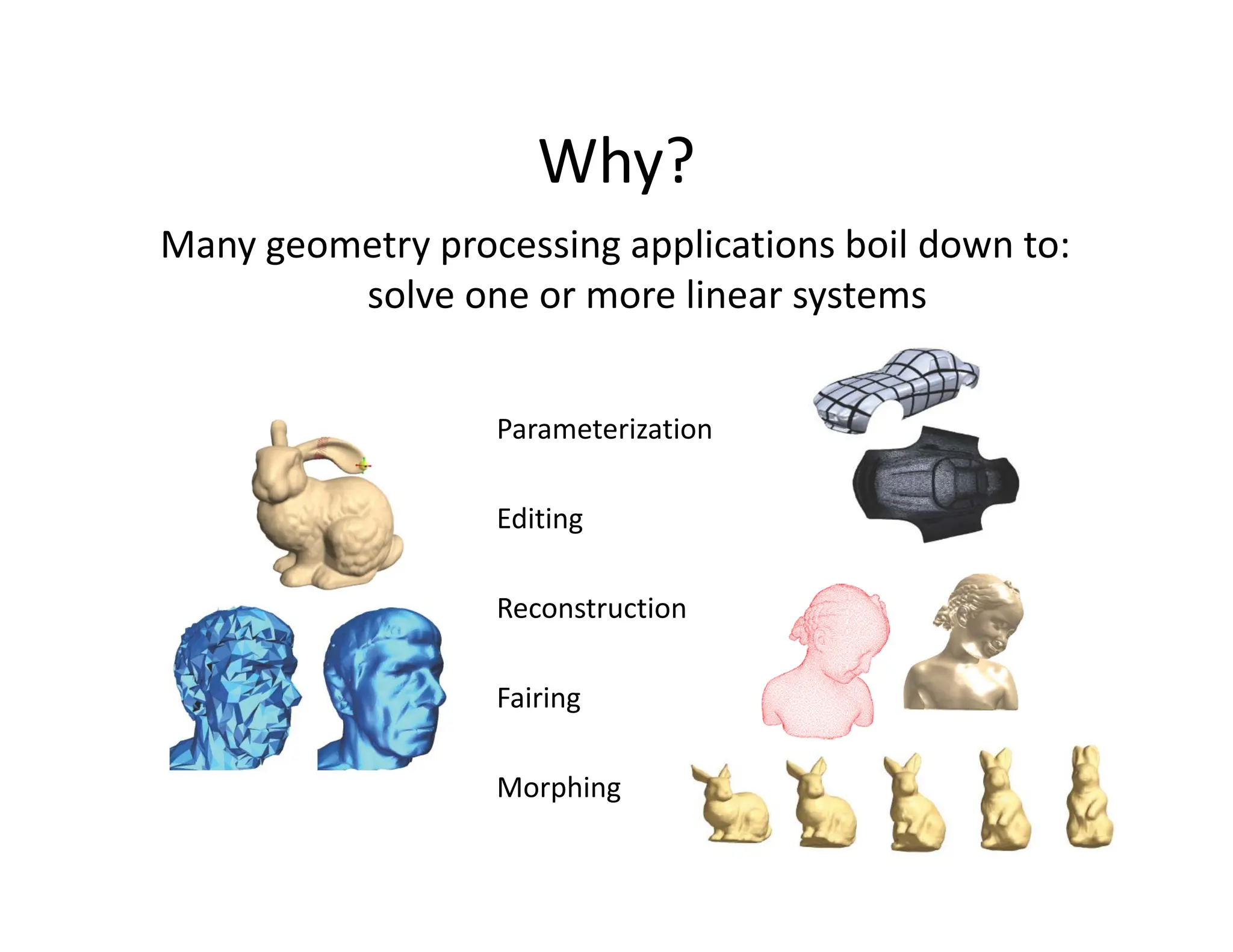
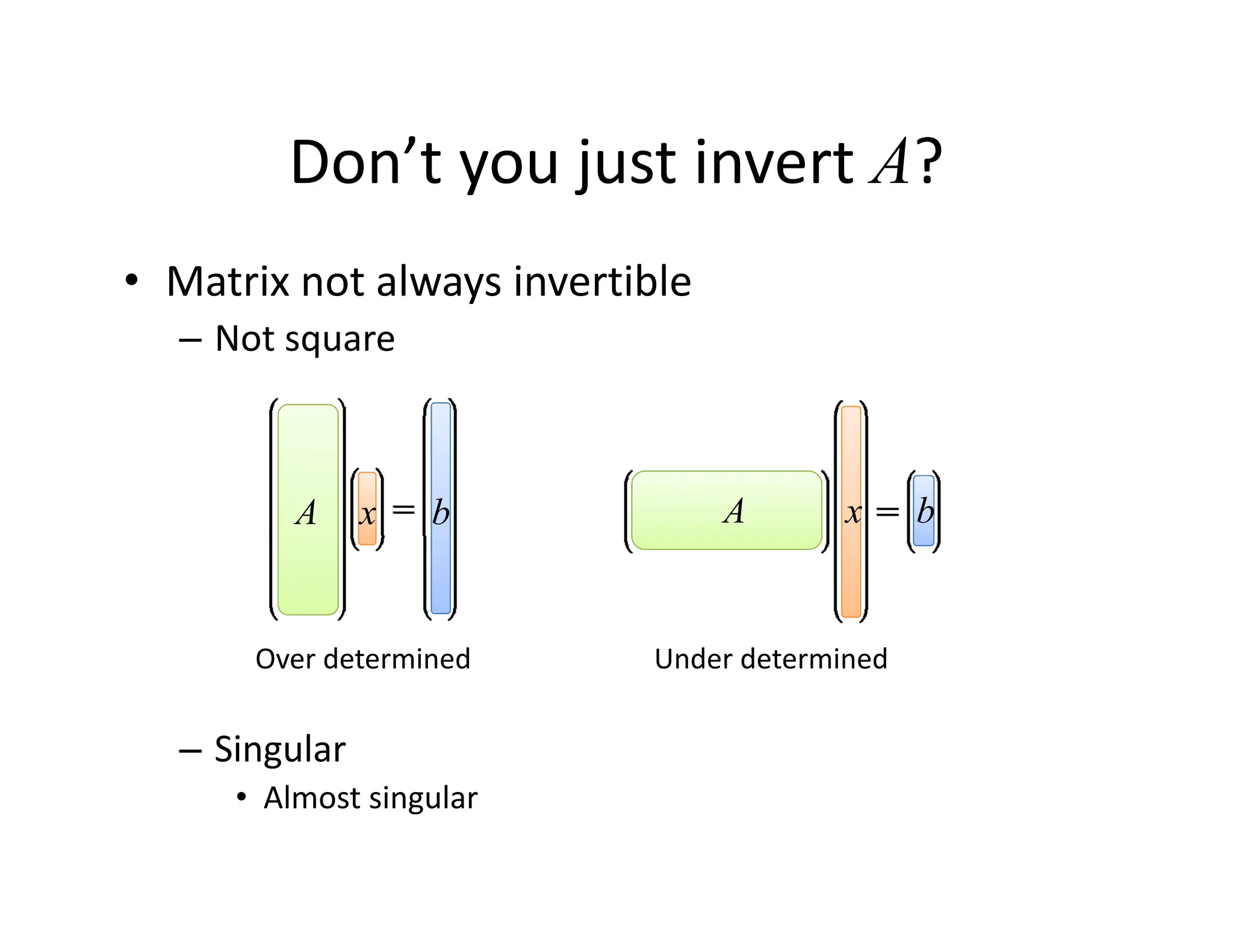
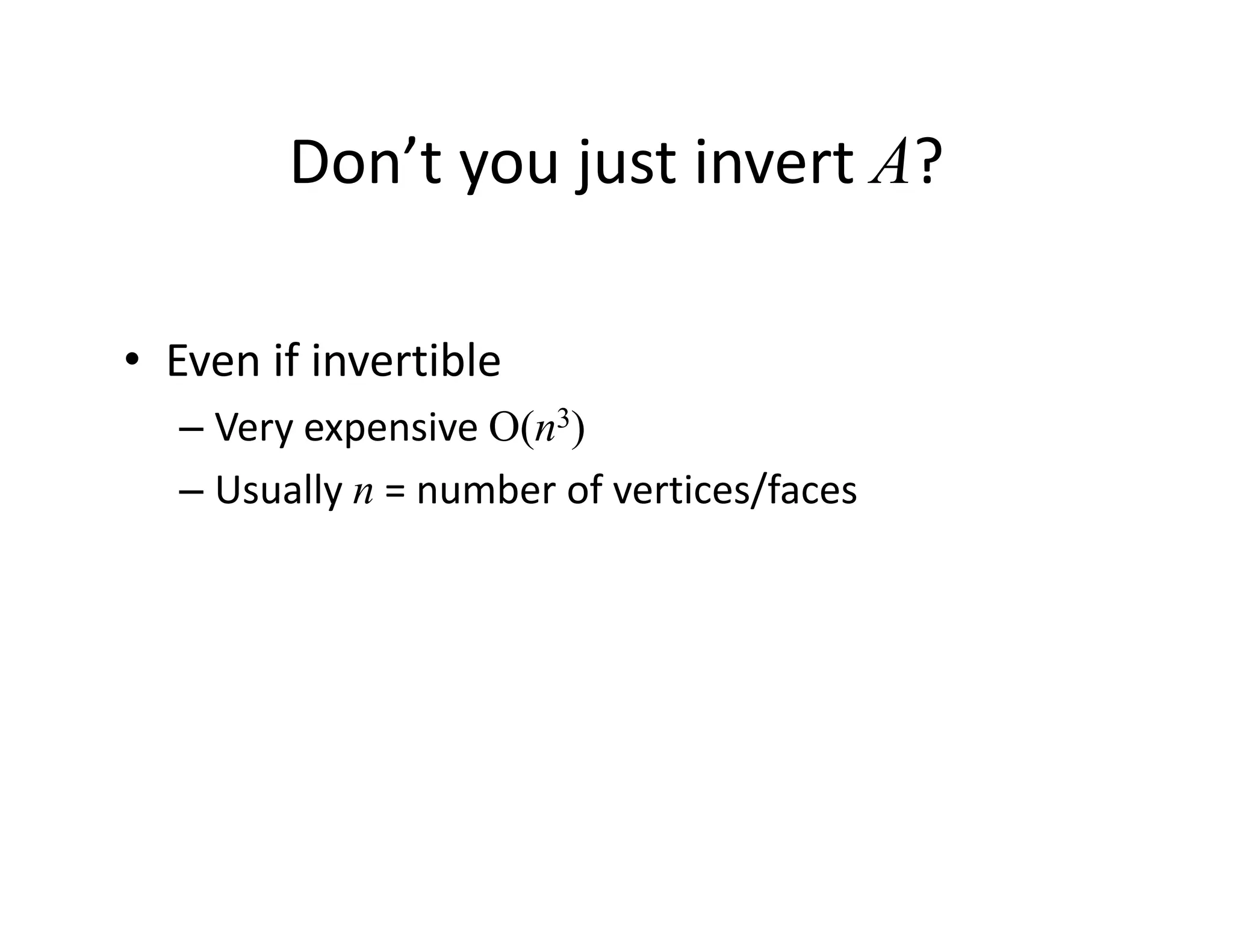
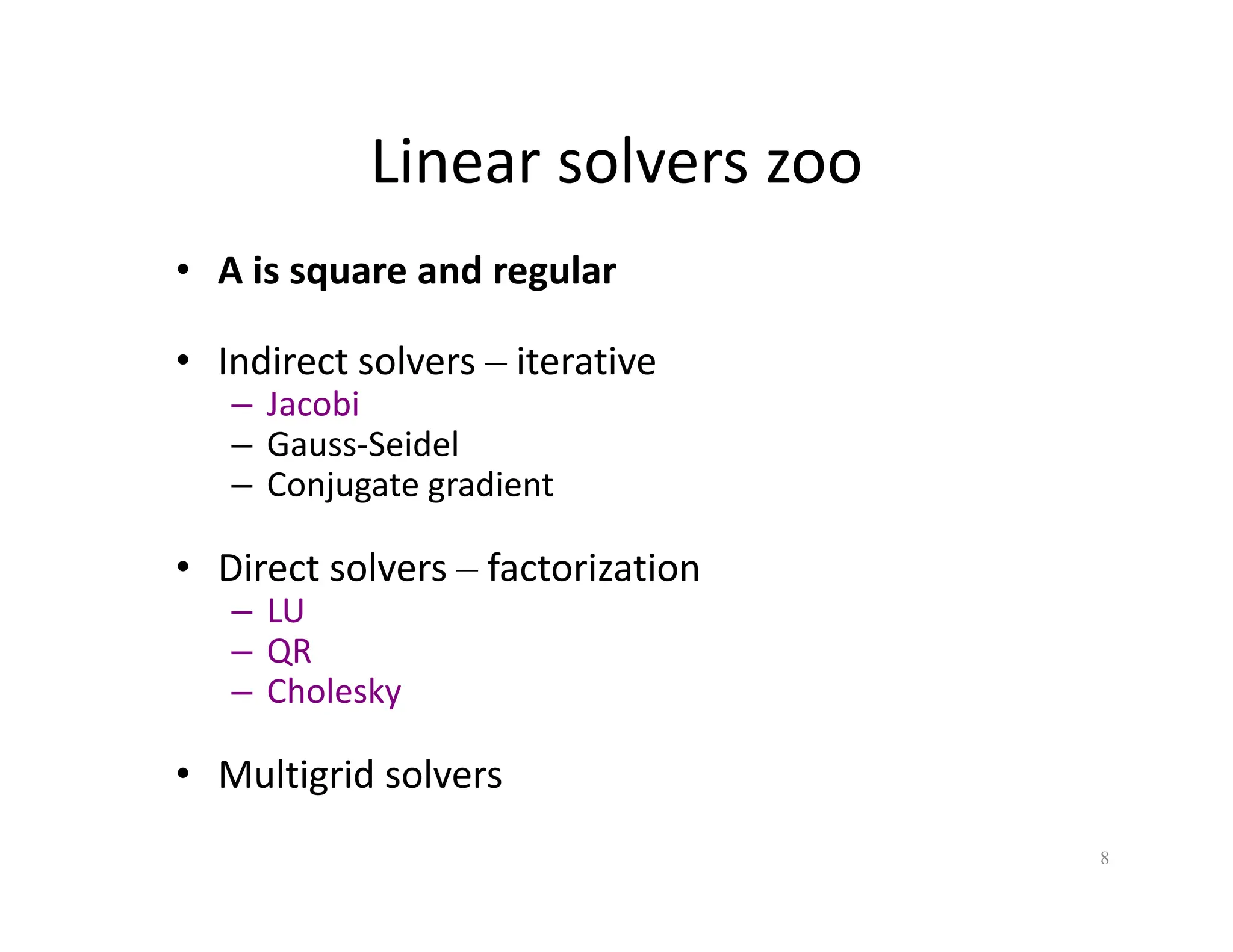
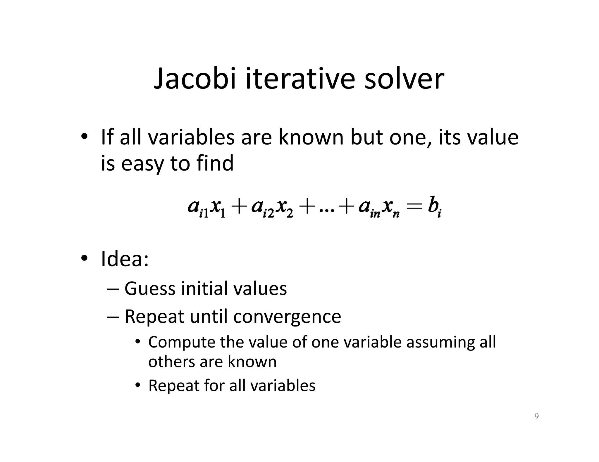
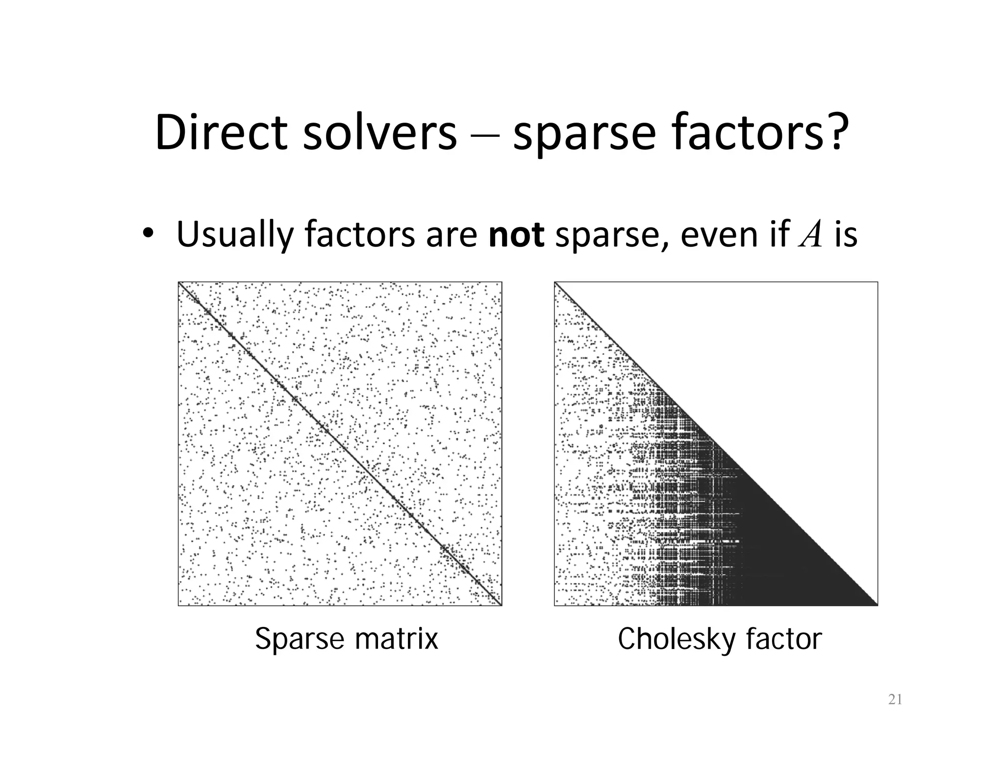
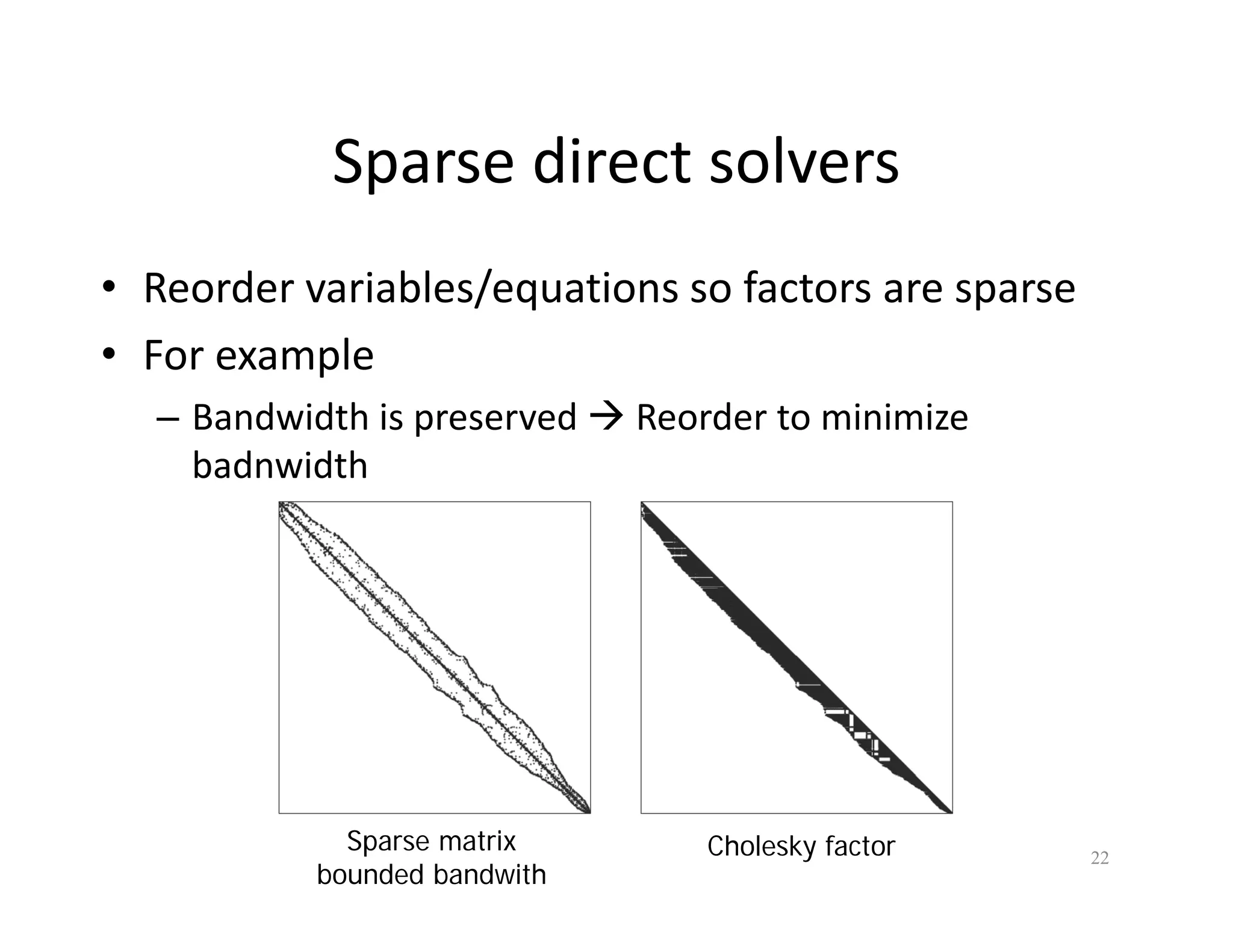
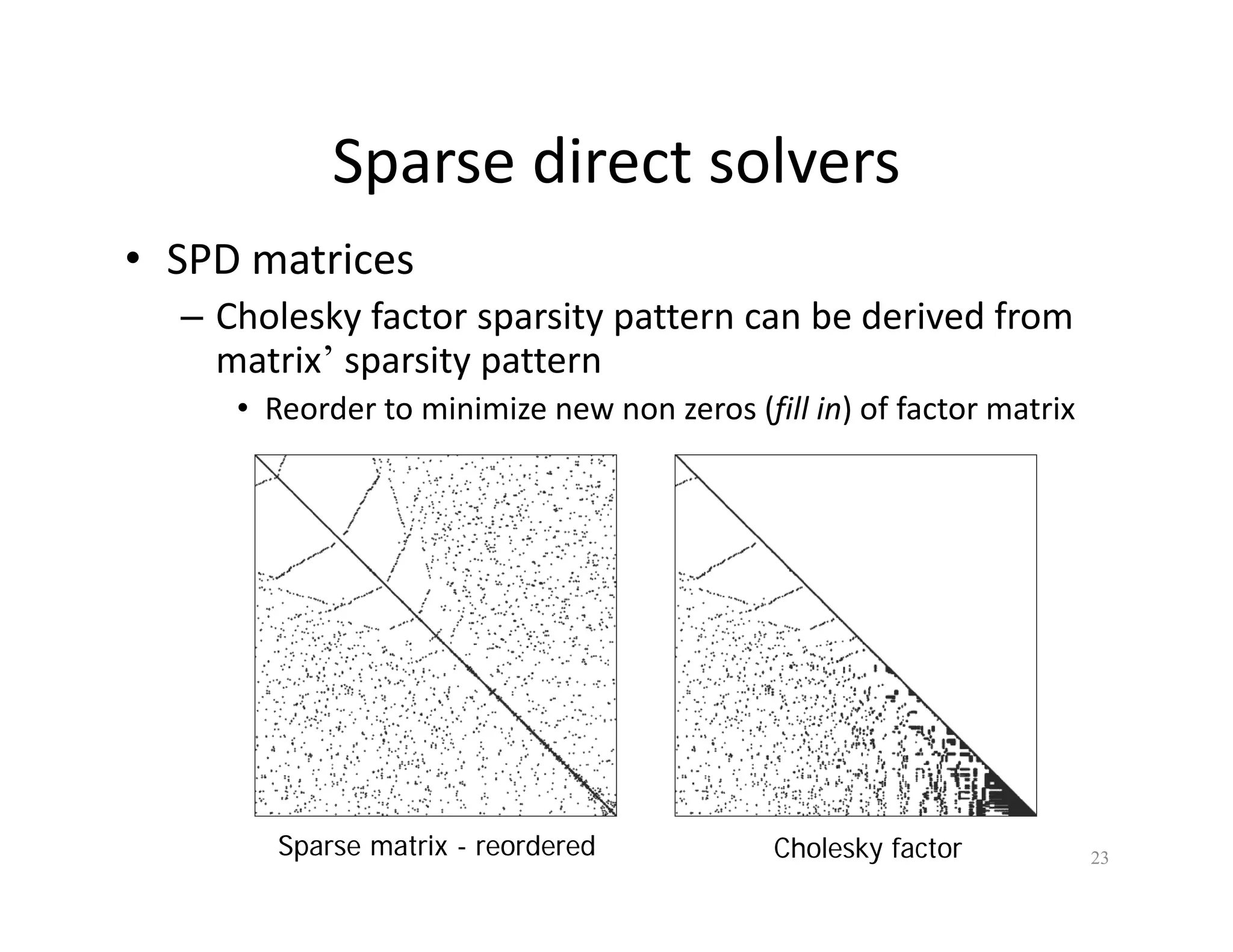
(Sparse) Linear Solvers
A B
A B
Ax = B
Ax = B
Why?
Why?
Many geometry processing applications boil down to:
solve one or more linear systems
Parameterization
Editing
Reconstruction
Fairing
Morphing
Don’t you just invert A?
• Matrix not always invertible
Don t you just invert A?
at ot a ays e t b e
– Not square
A x b A x b
Over determined Under determined
– Singular
Over determined Under determined
• Almost singular
Don’t you just invert A?
Don t you just invert A?
• Even if invertible
V i O( 3)
– Very expensive O(n3)
– Usually n = number of vertices/faces
Problem definition
• Input
Problem definition
– Matrix Amxn
– Vector Bmx1
• Output
– Vector xnx1
– Such that Ax = B
• Small time and memory complexity
• Use additional information on the problem
p
Properties of linear systems for DGP
• Sparse A
p
– Equations depend on
graph neighborhood
– Equations on vertices
Æ 7
Æ 7 non‐zeros per
row on average
– Number of non zero
elements O(n) n = 1002
( )
Non zeros = 7002
Properties of linear systems for DGP
• Symmetric positive definite (positive
y p (p
eigenvalues)
– Many times A is the Laplacian matrix
– Laplacian systems are usually SPD
• A remains, b changes – many right hand sides
– Interactive applications
– Mesh geometry – same matrix for X, Y, Z
Linear solvers zoo
Linear solvers zoo
• A is square and regular
• Indirect solvers – iterative
– Jacobi
Jacob
– Gauss‐Seidel
– Conjugate gradient
• Direct solvers – factorization
– LU
– QR
QR
– Cholesky
• Multigrid solvers
• Multigrid solvers
8
Jacobi iterative solver
• If all variables are known but one, its value
If all variables are known but one, its value
is easy to find
• Idea:
• Idea:
– Guess initial values
– Repeat until convergence
Repeat until convergence
• Compute the value of one variable assuming all
others are known
• Repeat for all variables
9
Jacobi iterative solver
• Let x* be the exact solution of Ax* = b
Let x be the exact solution of Ax b
• Jacobi method
– Set
– While not converged
Values from
previous iteration
• For i = 1 to n
previous iteration
10
Jacobi iterative solver
Pros
Si l t i l t
• Simple to implement
– No need for sparse data structure
• Low memory consumption O(n)
• Takes advantage of sparse structure
Takes advantage of sparse structure
b ll li d
• Can be parallelized
11
Jacobi iterative solver
Cons
• Guaranteed convergence for strictly diagonally
g y g y
dominant matrices
– The Laplacian is almost such a matrix
• Converges SLOWLY
• Converges SLOWLY
– Smoothens the error
– Once the error is smooth, slow convergence
• Doesn’t take advantage of
– Same A, different b
,
– SPD matrix
12
Direct solvers ‐ factorization
Direct solvers factorization
• If A is diagonal/triangular the system is easy to solve
If A is diagonal/triangular the system is easy to solve
• Idea:
• Idea:
– Factor A using “simple” matrices
x1
– Solve using k easy systems
13
Direct solvers ‐ factorization
Direct solvers factorization
• Factoring harder than solving
• Added benefit – multiple right hand sides
– Factor only once!
Factor only once!
14
Solving easy matrices
Diagonal
Diagonal
15
Solving easy matrices
Lower triangular
Lower triangular
• Forward substitution
• Start from x
• Start from x1
16
Solving easy matrices
Upper triangular
Upper triangular
• Backward substitution
• Start from x
• Start from xn
17
LU factorization
LU factorization
• A = LU
U
– L lower triangular
– U upper triangular
• Exists for any non‐singular square matrix
• Solve using Lx1=b and Ux = x1
18
QR factorization
QR factorization
• A = QR
A QR
– Q orthogonal Æ QT = Q -1
– R upper triangular
• Exists for any matrix
• Solve using Rx = QTb
19
Cholesky factorization
• A = LLT
– L lower triangular
• Exists for square symmetric positive definite
Exists for square symmetric positive definite
matrices
• Solve using Lx1=b and LTx = x1
20
Direct solvers – sparse factors?
Direct solvers sparse factors?
• Usually factors are not sparse even if A is
Usually factors are not sparse, even if A is
sparse
Sparse matrix Cholesk facto
21
Sparse matrix Cholesky factor
Sparse direct solvers
• Reorder variables/equations so factors are sparse
Reorder variables/equations so factors are sparse
• For example
Bandwidth is preserved Æ Reorder to minimize
– Bandwidth is preserved Æ Reorder to minimize
badnwidth
22
Sparse matrix
bounded bandwith
Cholesky factor
Sparse direct solvers
• SPD matrices
– Cholesky factor sparsity pattern can be derived from
matrix’ sparsity pattern
• Reorder to minimize new non zeros (fill in) of factor matrix
Reorder to minimize new non zeros (fill in) of factor matrix
23
Sparse matrix - reordered Cholesky factor
Sparse Cholesky
Sparse Cholesky
• Symbolic factorization
– Can be reused for matrix with same sparsity structure
• Even if values change!
O l f SPD i
• Only for SPD matrices
• Reordering is heuristic – not always gives good sparsity
g y g g p y
– High memory complexity if reordering was bad
• BUT
• BUT
– Works extremely well for Laplacian systems
– Can solve systems up to n = 500K on a standard PC
24
Under‐determined systems
Under determined systems
• System is under‐constrained Æ too many variables
• Solution: add constraints by pinning variables
– Add equations x1 = c1 , x2 = c2 , ... , xk = c2
Or
Or
– Replace variables with constants in equations
• Better smaller system
• Better – smaller system
25
Over‐determined systems
Over determined systems
• System is over‐constrained Æ too many
equations
• Unless equations are dependent, no solution
exists
• Instead, minimize:
26
Over‐determined systems
Over determined systems
• The minimizer of
• Is the solution of
• ATA is symmetric positive definite
– Can use Cholesky
Can use Cholesky
27
Singular square matrices
• Equivalent to under‐determined system
Equivalent to under determined system
dd i
• Add constraints
– By changing variables to constants
– NOT by adding equations!
• Will make system not square
• Much more expensive
28
Conclusions
Conclusions
• Many linear solvers exist
y
• Best choice depends on A
• DGP algorithms generate sparse SPD systems
• Research shows sparse linear solvers are best for DGP
• Sparse algs exist also for non‐square systems
• If solving in Matlab use “” operator
• If solving in Matlab – use “” operator
29
References
References
• “Efficient Linear System Solvers for Mesh
Efficient Linear System Solvers for Mesh
Processing”, Botsch et al., 2005
30

(Sparse) Linear solvers explanation1.pdf

  • 1.
    (Sparse) Linear Solvers AB A B Ax = B Ax = B
  • 2.
    Why? Why? Many geometry processingapplications boil down to: solve one or more linear systems solve one or more linear systems Parameterization Editing Reconstruction Fairing Morphing
  • 3.
    Don’t you justinvert A? • Matrix not always invertible Don t you just invert A? at ot a ays e t b e – Not square A x b A x b Over determined Under determined – Singular Over determined Under determined • Almost singular
  • 4.
    Don’t you justinvert A? Don t you just invert A? • Even if invertible V i O( 3) – Very expensive O(n3) – Usually n = number of vertices/faces
  • 5.
    Problem definition • Input Problemdefinition – Matrix Amxn – Vector Bmx1 • Output – Vector xnx1 – Such that Ax = B • Small time and memory complexity • Small time and memory complexity • Use additional information on the problem p
  • 6.
    Properties of linearsystems for DGP Properties of linear systems for DGP • Sparse A p – Equations depend on graph neighborhood – Equations on vertices Æ 7 Æ 7 non‐zeros per row on average – Number of non zero elements O(n) n = 1002 ( ) Non zeros = 7002
  • 7.
    Properties of linearsystems for DGP Properties of linear systems for DGP • Symmetric positive definite (positive y p (p eigenvalues) – Many times A is the Laplacian matrix – Laplacian systems are usually SPD • A remains, b changes – many right hand sides – Interactive applications – Mesh geometry – same matrix for X, Y, Z
  • 8.
    Linear solvers zoo Linearsolvers zoo • A is square and regular • Indirect solvers – iterative – Jacobi Jacob – Gauss‐Seidel – Conjugate gradient • Direct solvers – factorization – LU – QR QR – Cholesky • Multigrid solvers • Multigrid solvers 8
  • 9.
    Jacobi iterative solver Jacobiiterative solver • If all variables are known but one, its value If all variables are known but one, its value is easy to find • Idea: • Idea: – Guess initial values – Repeat until convergence Repeat until convergence • Compute the value of one variable assuming all others are known • Repeat for all variables 9
  • 10.
    Jacobi iterative solver Jacobiiterative solver • Let x* be the exact solution of Ax* = b Let x be the exact solution of Ax b • Jacobi method – Set – While not converged Values from previous iteration • For i = 1 to n previous iteration 10
  • 11.
    Jacobi iterative solver Pros Sil t i l t • Simple to implement – No need for sparse data structure • Low memory consumption O(n) • Takes advantage of sparse structure Takes advantage of sparse structure b ll li d • Can be parallelized 11
  • 12.
    Jacobi iterative solver Cons •Guaranteed convergence for strictly diagonally g y g y dominant matrices – The Laplacian is almost such a matrix • Converges SLOWLY • Converges SLOWLY – Smoothens the error – Once the error is smooth, slow convergence • Doesn’t take advantage of – Same A, different b , – SPD matrix 12
  • 13.
    Direct solvers ‐factorization Direct solvers factorization • If A is diagonal/triangular the system is easy to solve If A is diagonal/triangular the system is easy to solve • Idea: • Idea: – Factor A using “simple” matrices x1 – Solve using k easy systems 13
  • 14.
    Direct solvers ‐factorization Direct solvers factorization • Factoring harder than solving • Factoring harder than solving • Added benefit – multiple right hand sides – Factor only once! Factor only once! 14
  • 15.
    Solving easy matrices Solvingeasy matrices Diagonal Diagonal 15
  • 16.
    Solving easy matrices Solvingeasy matrices Lower triangular Lower triangular • Forward substitution • Start from x • Start from x1 16
  • 17.
    Solving easy matrices Solvingeasy matrices Upper triangular Upper triangular • Backward substitution • Start from x • Start from xn 17
  • 18.
    LU factorization LU factorization •A = LU U – L lower triangular – U upper triangular • Exists for any non‐singular square matrix • Solve using Lx1=b and Ux = x1 18
  • 19.
    QR factorization QR factorization •A = QR A QR – Q orthogonal Æ QT = Q -1 – R upper triangular • Exists for any matrix • Solve using Rx = QTb 19
  • 20.
    Cholesky factorization Cholesky factorization •A = LLT – L lower triangular • Exists for square symmetric positive definite Exists for square symmetric positive definite matrices • Solve using Lx1=b and LTx = x1 20
  • 21.
    Direct solvers –sparse factors? Direct solvers sparse factors? • Usually factors are not sparse even if A is Usually factors are not sparse, even if A is sparse Sparse matrix Cholesk facto 21 Sparse matrix Cholesky factor
  • 22.
    Sparse direct solvers Sparsedirect solvers • Reorder variables/equations so factors are sparse Reorder variables/equations so factors are sparse • For example Bandwidth is preserved Æ Reorder to minimize – Bandwidth is preserved Æ Reorder to minimize badnwidth 22 Sparse matrix bounded bandwith Cholesky factor
  • 23.
    Sparse direct solvers Sparsedirect solvers • SPD matrices – Cholesky factor sparsity pattern can be derived from matrix’ sparsity pattern • Reorder to minimize new non zeros (fill in) of factor matrix Reorder to minimize new non zeros (fill in) of factor matrix 23 Sparse matrix - reordered Cholesky factor
  • 24.
    Sparse Cholesky Sparse Cholesky •Symbolic factorization – Can be reused for matrix with same sparsity structure • Even if values change! O l f SPD i • Only for SPD matrices • Reordering is heuristic – not always gives good sparsity g y g g p y – High memory complexity if reordering was bad • BUT • BUT – Works extremely well for Laplacian systems – Can solve systems up to n = 500K on a standard PC 24
  • 25.
    Under‐determined systems Under determinedsystems • System is under‐constrained Æ too many variables • Solution: add constraints by pinning variables • Solution: add constraints by pinning variables – Add equations x1 = c1 , x2 = c2 , ... , xk = c2 Or Or – Replace variables with constants in equations • Better smaller system • Better – smaller system 25
  • 26.
    Over‐determined systems Over determinedsystems • System is over‐constrained Æ too many equations • Unless equations are dependent, no solution exists • Instead, minimize: 26
  • 27.
    Over‐determined systems Over determinedsystems • The minimizer of • Is the solution of • ATA is symmetric positive definite – Can use Cholesky Can use Cholesky 27
  • 28.
    Singular square matrices Singularsquare matrices • Equivalent to under‐determined system Equivalent to under determined system dd i • Add constraints – By changing variables to constants – NOT by adding equations! • Will make system not square • Much more expensive 28
  • 29.
    Conclusions Conclusions • Many linearsolvers exist y • Best choice depends on A • DGP algorithms generate sparse SPD systems • Research shows sparse linear solvers are best for DGP • Sparse algs exist also for non‐square systems • If solving in Matlab use “” operator • If solving in Matlab – use “” operator 29
  • 30.
    References References • “Efficient LinearSystem Solvers for Mesh Efficient Linear System Solvers for Mesh Processing”, Botsch et al., 2005 30