This document contains three classical mechanics homework problems involving motion under the influence of forces. Problem 1 considers vertical motion affected by gravity and air resistance. Problem 2 examines motion down an inclined plane with friction. Problem 3 analyzes the trajectory of a charged particle moving in crossed electric and magnetic fields.
![Classical Mechanics Homework 2
Due October 12, 2012
1. (Taylor, Problem 2-11) Consider an object that is thrown vertically up
with initial speed v0 in a linear medium.
StatementThis is another problem in which we consider the effects of air
resistance on motion under gravity. In this case we need to find the height
as a function of time going up, starting with some initial velocity.
AssumptionsWe assume linear drag plus gravity, and linear motion. The
object is a point particle.
Physical representationThe forces we need are gravity pointing down,
hence negative, and drag pointing down, also negative. We consider mo-
tion going up only, and do not worry what happens after we reach the top
of the orbit.
Mathematical representation and solutionMathematical representa-
tion and solution, see parts below.
(a) Measuring y upward from the point of release, write expressions for
the object’s velocity vy (t) and position y(t).
This follows exactly what we did in class. Starting with an expression
for Newton’s 2nd Law (coordinate system positive upward):
mv
˙ = −mg − bv
∫ v ∫ t
m
dv ′ = − dt′
v0 mg + bv ′ 0
( )
m mg + bv
− ln = t
b mg + bv0
( mg ) mg
v = + v0 e−bt/m −
b b
Now, separate again to find position as a function of time:
∫ y ∫ t [( )
′ mg ′ mg ] ′
dy = + v0 e−bt /m − dt
y0 0 b b
m ( mg )( ) mg
y − y0 = + v0 1 − e−bt/m − t
b b b
(b) Find the time for the object to reach its highest point and its position
ymax at that point.](https://image.slidesharecdn.com/solution33-130304232921-phpapp02/85/Solution-3-3-1-320.jpg)
![Classical Mechanics Homework 2
Due October 12, 2012
1. (Taylor, Problem 2-11) Consider an object that is thrown vertically up
with initial speed v0 in a linear medium.
StatementThis is another problem in which we consider the effects of air
resistance on motion under gravity. In this case we need to find the height
as a function of time going up, starting with some initial velocity.
AssumptionsWe assume linear drag plus gravity, and linear motion. The
object is a point particle.
Physical representationThe forces we need are gravity pointing down,
hence negative, and drag pointing down, also negative. We consider mo-
tion going up only, and do not worry what happens after we reach the top
of the orbit.
Mathematical representation and solutionMathematical representa-
tion and solution, see parts below.
(a) Measuring y upward from the point of release, write expressions for
the object’s velocity vy (t) and position y(t).
This follows exactly what we did in class. Starting with an expression
for Newton’s 2nd Law (coordinate system positive upward):
mv
˙ = −mg − bv
∫ v ∫ t
m
dv ′ = − dt′
v0 mg + bv ′ 0
( )
m mg + bv
− ln = t
b mg + bv0
( mg ) mg
v = + v0 e−bt/m −
b b
Now, separate again to find position as a function of time:
∫ y ∫ t [( )
′ mg ′ mg ] ′
dy = + v0 e−bt /m − dt
y0 0 b b
m ( mg )( ) mg
y − y0 = + v0 1 − e−bt/m − t
b b b
(b) Find the time for the object to reach its highest point and its position
ymax at that point.](https://image.slidesharecdn.com/solution33-130304232921-phpapp02/75/Solution-3-3-1-2048.jpg)
![mdv ′
= dt′
mg sin(θ) − kmv ′ 2
Note that as usual the mass of the object drops out! Gravity and acceler-
ation always contain mass in the same manner.
dv ′
= dt′
g sin(θ) − kv ′ 2
Integrating:
∫ ∫
v
dv ′ t
= dt′
0 g sin θ − kv ′ 2 0
∫ ∫
1 v
dv ′ t
− = dt′
k 0 v ′ − c2
2
0
where we have defined
g
sin(θ) c2 =
k
∫ v[ ] ∫ t
1 dv ′ dv ′
− − ′ = dt′
2ck 0 v ′ − c v + c 0
1
−
[ln(|v − c|) − ln(c) − ln(v + c) + ln(c)] = t
2ck
We know that we have v < c, we never reach terminal velocity. Therefore
c−v
ln( ) = −2ckt
c+v
Solve for v so that I can find the distance:
(c − v) = (c + v)e−2ckt
v(1 + e−2ckt ) = c(1 − e−2ckt )
1 − e−2ckt
v=c
1 + e−2ckt
√ (√ )
g sin θ
v = tanh t kg sin θ
k
∫ d ∫ t √ ( √ )
g sin θ
dx′ = tanh t′ kg sin θ dt′
0 0 k
√ [ ( √ )]
g sin θ 1 t
d = √ ln cosh t′ kg sin θ
k kg sin θ 0
1 [ (√ )]
d = ln cosh t kg sin θ
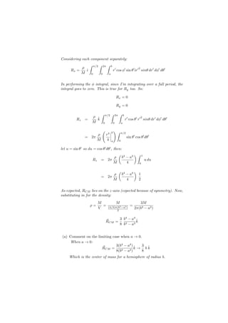
k](https://image.slidesharecdn.com/solution33-130304232921-phpapp02/85/Solution-3-3-4-320.jpg)
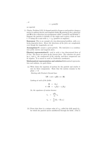
![Solving for t:
(√ )
ekd = cosh t kg sin θ
cosh−1 ekd
t = √
kg sin θ
This part of the question was not asked, but is a useful example. Using:
2
k = 0.5 N/(m/s)
π
θ = radians
3
0.7
0.6
0.5
Time, t [s] 0.4
0.3
0.2
0.1
0
0 0.5 1.0 1.5 2.0
Distance , d m
Quadratic Drag No Drag
For the no drag case: √
2d
t=
g sin θ
The plot shows that the no drag case reaches a larger distance in the same
amount of time.
Evaluation In order to make sense of the results we do have to look at
the extra parts. With friction we travel a smaller distance than without,
which is expected. Also, in the limit of zero friction we have from
1 − e−2ckt
v=c
1 + e−2ckt
that
2ckt
v≈c = c2 kt
1+1](https://image.slidesharecdn.com/solution33-130304232921-phpapp02/85/Solution-3-3-5-320.jpg)
![the basis of velocity selectors, which select particles traveling at one
chosen speed from a beam with many different speeds.)
For there to be no deflection, the force in the y-direction must be
zero.
ΣFy = q(E0 − B0 vx )
0 = q(E0 − B0 vx )
E0
vx =
B0
E0
vdr =
B0
(c) Solve the equations of motion to give the particle’s velocity as a
function of t, for arbitrary values of vx0 . [Hint: The equations for
(vx , vy ) should look very much like Equations (2.86) except for an
offset of vx by a constant. If you make a change of variables of the
form ux = vx − vdr and uy = vy , the equations for (ux , uy ) will have
exactly the form (2.68), whose general solution you know.]
Letting
ux = vx − vdr
uy = vy
The equations of motion become:
qB0
ux
˙ = uy
m
qB0
uy
˙ = − ux
m
Taking another time derivative of the x equation yields:
qB0
ux =
¨ uy
˙
m
Now, substituting the original equation of motion:
qB0
ux
¨ = − ux
m
ux = A sin ω t + B cos ω t](https://image.slidesharecdn.com/solution33-130304232921-phpapp02/85/Solution-3-3-7-320.jpg)
![vx = A sin ω t + B cos ω t + vdr
qB0
where ω = m This gives
u˙x = Aω cos(ωt) − Bω sin(ωt)
qB0
uy = Aω cos(ωt) − Bω sin(ωt)
m
Using the initial condition that uy (t = 0) = 0 gives A = 0. Using the
initial condition that vx (t = 0) = vx0 :
vx0 = B + vdr
B = vx0 − vdr
vx = (vx0 − vdr ) cos ω t + vdr
Now, using this result to find the vy
qB0
uy
˙ = − ux
m
qB0
vy
˙ = − (vx − vdr )
m
qB0
vy
˙ = − (vx0 − vdr ) cos ω t
m
∫ vy ∫ t
′
dvy = −ω(vx0 − vdr ) cos ω t′ dt′
0 0
vy = −(vx0 − vdr ) sin ω t
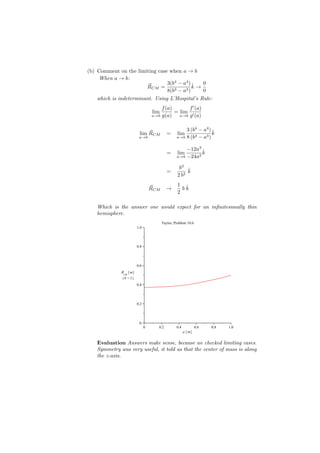
(d) Integrate the velocity to find the position as a function of t and sketch
the trajectory for various values of vx0
The integration is straightforward:
vx = (vx0 − vdr ) cos (ω t) + vdr
∫ x ∫ t
dx′ = [(vx0 − vdr ) cos (ω t′ ) + vdr ] dt′
x0 0
[ ] t
vx0 − vdr
x − x0 = sin (ω t′ ) + vdr t′
ω 0
vx0 − vdr
x − x0 = sin (ω t) + vdr t
ω](https://image.slidesharecdn.com/solution33-130304232921-phpapp02/85/Solution-3-3-8-320.jpg)
![vy = −(vx0 − vdr ) sin (ω t)
∫ y ∫ t
′
dy = − (vx0 − vdr ) sin (ω t′ ) dt′
y0 0
t
vx0 − vdr
y − y0 = cos (ω t′ )
ω 0
vx0 − vdr
y − y0 = [cos (ω t) − 1]
ω
Trajectories can be oscillatory or run back.
0.0 2.5 5.0 7.5 10.0 12.5
0.0
−0.5
−1.0
−1.5
−2.0
Evaluation We found several familiar results. The condition for no de-
flection was found in Ph213, as was the cyclotron frequency. We can
also set the electric field equal to zero, which gives vdr = 0 and the orbit
becomes a circle as expected.
4. (Thorton & Marion, Problem 9-60) A rocket has an initial mass of 7 × 10⁴
kg and on firing burns its fuel at a rate of 250 kg/s. The exhaust velocity
is 2500 m/s. If the rocket has a vertical ascent from rest on the earth, how
long after the rocket engines fire will the rocket lift off? What is wrong
with the design of this rocket?
StatementAn application of what we did in class, but now using realistic
numbers. We are asked about the conditions for lift-off for a rocket, and
need to check if the thrust is strong enough.
AssumptionsThe fuel is spent at a constant rate, and we do not take
into account how the exhaust gas hits the launch pad.](https://image.slidesharecdn.com/solution33-130304232921-phpapp02/85/Solution-3-3-9-320.jpg)
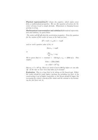
![30
20
t [s]
liftoff
10
K K K K
0
280 270 260 250
dm kg
dt s
5. (Taylor, Problem 10.6) Find the CM of a uniform hemispherical shell of
inner and outer radii a and b and mass M .
Statement This problem asks us to evaluate the center of mass.
AssumptionsWe have a hemispherical shell with constant mass density.
Physical representationThis problem seems like it works best with spher-
ical coordinates. We take the x and y axis along the plane of the cut, and
have the z-axis pointing upwards through the hemisphere. This represen-
tations makes full use of the symmetry of the problem.
Mathematical representation and solutionMathematical representa-
tion and solution, see parts below.
I’m going to place my origin of coordinates at the center of the sphere.
Using spherical coordinates:
∫
1
⃗
RCM = ρ(⃗′ ) ⃗′ dτ ′
r r
M
∫ ∫ ∫
1
ρ(⃗′ ) ⃗′ r′ dr′ sinθ dϕ′ dθ′
2
= r r
M
⃗
r ˆ
= r cos ϕ sin θˆ + r sin ϕ sin θˆ + r cos θk
ı ȷ
ρ(⃗′ ) =
r ρ
∫ π/2 ∫ 2π ∫ b [ ]
ρ
⃗
RCM = r′ cos ϕ′ sin θ′ˆ + r′ sin ϕ′ sin θ′ ȷ + r′ cos θ′ k r′ sinθ dr′ dϕ′ dθ′
ı ˆ ˆ 2
M 0 0 a](https://image.slidesharecdn.com/solution33-130304232921-phpapp02/85/Solution-3-3-11-320.jpg)