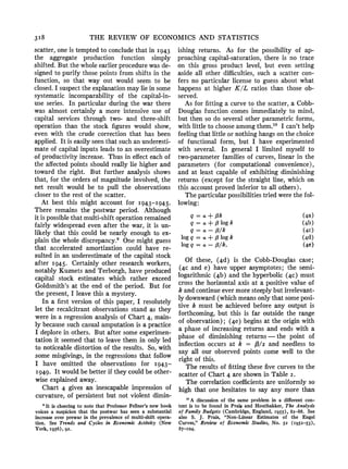
- The document discusses using an aggregate production function to isolate the effects of technical change on output over time.
- It presents a method for estimating an index of technical change (A(t)) based on time series data for output per worker, capital per worker, and the share of capital, using the assumption that factors are paid their marginal products.
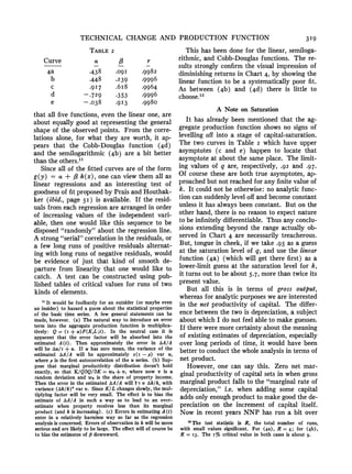
- The method is applied to U.S. data from 1909-1949 to generate an estimated index of technical change, which increased steadily over that period.


![TECHNICAL CHANGE AND THE AGGREGATE
PRODUCTION FUNCTION *
Robert M. Solow
JN this day of rationallydesignedeconometric
studies and super-input-output tables, it
takes something more than the usual "willing
suspensionof disbelief" to talk seriouslyof the
aggregateproduction function. But the aggre-
gate production function is only a little less
legitimate a concept than, say, the aggregate
consumption function, and for some kinds of
long-run macro-models it is almost as indis-
pensable as the latter is for the short-run. As
long as we insist on practicingmacro-economics
we shall need aggregaterelationships.
Even so, therewould hardly be any justifica-
tion for returningto this old-fashionedtopic if
I had no novelty to suggest. The new wrinkle
I want to describe is an elementary way of
segregatingvariationsin outputper head dueto
technical change from those due to changes in
the availability of capital per head. Naturally,
every additional bit of information has its
price. In this case the price consists of one new
requiredtime series, the share of laboror prop-
erty in total income, and one new assumption,
that factors are paid their marginalproducts.
Since the former is probably more respectable
than the other data I shall use, and since the
latter is an assumption often made, the price
may not be unreasonablyhigh.
Before going on, let me be explicit that I
wouldnot try to justify what follows by calling
on fancy theorems on aggregation and index
numbers.' Either this kind of aggregate eco-
nomics appeals or it doesn't. Personally I be-
long to both schools. If it does, I think one can
draw some crude but useful conclusions from
the results.
TheoreticalBasis
I will first explain what I have in mind
mathematicallyand then give a diagrammatic
exposition. In this case the mathematicsseems
simpler. If Q represents output and K and L
representcapital and laborinputs in "physical"
units, then fhe aggregate production function
can be written as:
Q = F(K,L;t). (I)
The variable t for time appears in F to allow
for technical change. It will be seen that I am
using the phrase "technicalchange"as a short-
hand expression for any kind of shift in the
production function. Thus slowdowns, speed-
ups,improvementsin the educationof the labor
force, and all sorts of things will appear as
"technicalchange."
It is convenientto begin with the specialcase
of neutral technical change. Shifts in the pro-
duction function are definedas neutral if they
leave marginalrates of substitution untouched
but simply increase or decrease the output at-
tainable from given inputs. In that case the
productionfunctiontakes the special form
Q = A(t)f (K,L4) (ia)
and the multiplicativefactorA(t) measuresthe
cumulatedeffectof shifts over time. Differenti-
ate (ia) totally with respectto time and divide
by Q and one obtains
? A DJa.K DIL
=+ A - +A -
Q A DK Q DL Q
where dots indicate time derivatives. Now de-
fine wk -3Q K
andWL= aQ
L
the rela-
DK Q DL Q
tive shares of capital and labor, and substitute
in the above equation (note that DQ/DK=
A Df/3K, etc.) andthereresults:
-+WK-+WL ~~~~~(2)Q A K L
* I owe a debt of gratitude to Dr. Louis Lefeber for sta-
tistical and other assistance, and to Professors Fellner,
Leontief, and Schultz for stimulating suggestions.
1 Mrs. Robinson in particular has explored many of the
profound difficulties that stand in the way of giving any
precise meaning to the quantity of capital ("The Production
Function and the Theory of Capital," Review of Economic
Studies, Vol. 2I, No. 2), and I have thrown up still further
obstacles (ibid., Vol. 23, No. 2). Were the data available, it
would be better to apply the analysis to some precisely de-
fined production function with many precisely defined in-
puts. One can at least hope that the aggregate analysis
gives some notion of the way a detailed analysis would
lead.
[ 3I2 ]](https://image.slidesharecdn.com/solow1957-101108183053-phpapp02/85/Solow1957-2-320.jpg)