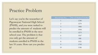
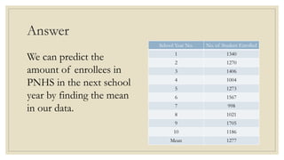
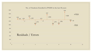
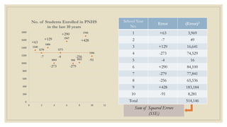
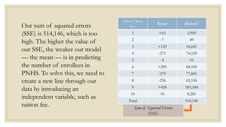
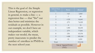
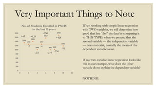
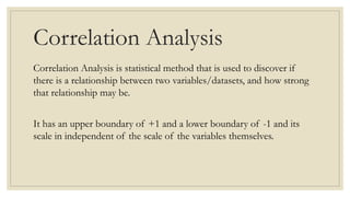
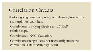
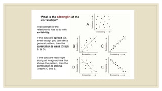
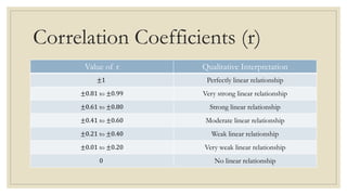
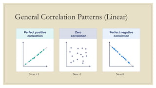
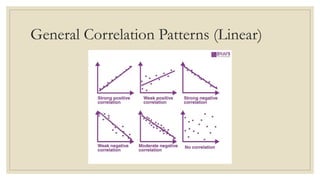
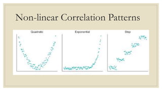
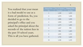
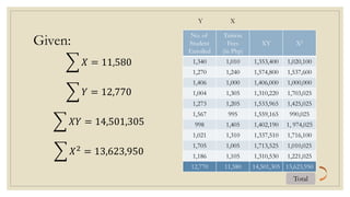
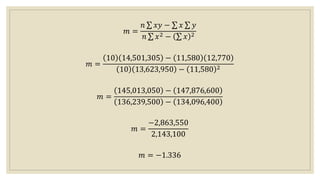
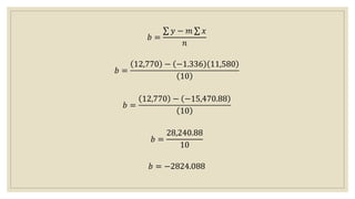
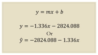
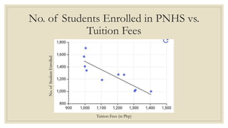
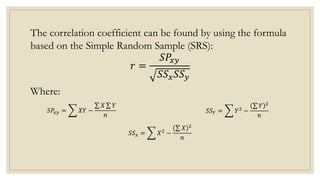
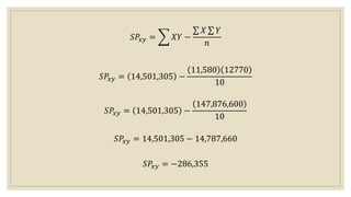
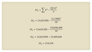
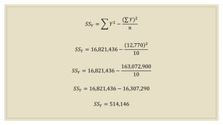
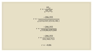
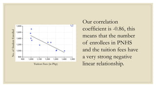
This document discusses simple linear regression and correlation analysis. It begins by explaining simple linear regression as focusing on the relationship between two variables. It then provides an example using data on student enrollment in a school over 10 years to predict future enrollment. Several methods of simple linear regression are demonstrated, including finding the slope and y-intercept of the regression line. The document then discusses correlation analysis, explaining it as a measure of the strength and direction of the linear relationship between two variables. Different correlation coefficients and their interpretations are provided. Finally, it returns to the student enrollment example to calculate the correlation between enrollment and tuition fees, finding a strong negative correlation between the two variables.

1. SIMPLE LINEAR
REGRESSION AND
CORRELATION ANALYSIS
Understanding and Calculation

2. UNDERSTANDING
SIMPLE LINEAR
REGRESSION
Understanding the Concepts Behind It

3. Simple Linear Regression Analysis
The simple linear regression analysis is
one of the types of linear regression that
focuses on the relationship of TWO
VARIABLES, the other type being
Multiple Linear Regression.

4. Practice Problem
Let's say you're the researcher of
Pigcawayan National High School
(PNHS), and you were tasked to
predict the amount of students will
be enrolled in PNHS in the next
school year. The problem is that
you only get the amount of
students enrolled in PNHS in the
last 10 years. How can you predict
it?
School Year No. No. of Student Enrolled
1 1340
2 1270
3 1406
4 1004
5 1273
6 1567
7 998
8 1021
9 1705
10 1186

5. Answer
We can predict the
amount of enrollees in
PNHS in the next school
year by finding the mean
in our data.
School Year No. No. of Student Enrolled
1 1340
2 1270
3 1406
4 1004
5 1273
6 1567
7 998
8 1021
9 1705
10 1186
Mean 1277

6. 1340
1270
1406
1004
1273
1567
998 1021
1705
1186
0
200
400
600
800
1000
1200
1400
1600
1800
0 2 4 6 8 10 12
No. of Students Enrolled in PNHS in the last 10 years
+63 +129
+290
+428
-7 -273
-4
-279 -256 -91
-910
+910
Residuals / Errors

7. School Year
No.
Error (Error)2
1 +63 3,969
2 -7 49
3 +129 16,641
4 -273 74,529
5 -4 16
6 +290 84,100
7 -279 77,841
8 -256 65,536
9 +428 183,184
10 -91 8,281
Total 514,146
1340
1270
1406
1004
1273
1567
998 1021
1705
1186
0
200
400
600
800
1000
1200
1400
1600
1800
0 2 4 6 8 10 12
No. of Students Enrolled in PNHS
in the last 10 years
+63
-7
+129
-273
-4
+290
-279
-256
+428
-91
Sum of Squared Errors
(SSE)

8. School Year
No.
Error (Error)2
1 +63 3,969
2 -7 49
3 +129 16,641
4 -273 74,529
5 -4 16
6 +290 84,100
7 -279 77,841
8 -256 65,536
9 +428 183,184
10 -91 8,281
Total 514,146
Sum of Squared Errors
(SSE)
Our sum of squared errors
(SSE) is 514,146, which is too
high. The higher the value of
our SSE, the weaker our model
— the mean — is in predicting
the number of enrollees in
PNHS. To solve this, we need to
create a new line through our
data by introducing an
independent variable, such as
tuition fee.

9. School Year
No.
Error (Error)2
1 +63 3,969
2 -7 49
3 +129 16,641
4 -273 74,529
5 -4 16
6 +290 84,100
7 -279 77,841
8 -256 65,536
9 +428 183,184
10 -91 8,281
Total 514,146
Sum of Squared Errors
(SSE)
This is the goal of the Simple
Linear Regression, or regression
in general, to make a line — a
regression line — that "fits" our
data better and minimize the
residuals as possible. However in
our example, we don't have an
independent variable, which
makes our model, the mean,
pretty inaccurate to predict the
number of enrollees in PNHS in
the next school year.

10. 1340
1270
1406
1004
1273
1567
998 1021
1705
1186
0
200
400
600
800
1000
1200
1400
1600
1800
0 2 4 6 8 10 12
No. of Students Enrolled in PNHS
in the last 10 years
+63
-7
+129
-273
-4
+290
-279
-256
+428
-91
When working with simple linear regression
with TWO variables, we will determine how
good that line “fits” the data by comparing it
to THIS TYPE: when we pretend that the
second variable — the independent variable
— does not exist, basically the mean of the
dependent variable alone.
If our two-variable linear regression looks like
this in our example, what does the other
variable do to explain the dependent variable?
NOTHING.
Very Important Things to Note

11. Quick Review
◦ Simple linear regression is really a comparison of two models:
a) One is where the independent variable does not exists.
b) And the other uses the best-fit regression line.
◦ If there is only one variable, the best prediction of other values is the mean of
the dependent variable.
◦ The distance between the best-fit line to the observed value is called the residual
or error.
◦ The residuals are squared and summed to create the Sum of Squared Residuals /
Error (SSE).
◦ The simple linear regression is designed to make a line best fits our data and
minimize the number of SSE.

12. UNDERSTANDING
CORRELATION
ANALYSIS
Understanding the Concepts Behind It

13. Correlation Analysis
Correlation Analysis is statistical method that is used to discover if
there is a relationship between two variables/datasets, and how strong
that relationship may be.
It has an upper boundary of +1 and a lower boundary of -1 and its
scale in independent of the scale of the variables themselves.

14. Correlation Caveats
◦Before going crazy computing correlations, look at the
scatterplot of your data.
◦Correlations is only applicable to LINEAR
relationships.
◦Correlation is NOT Causation.
◦Correlation strength does not necessarily mean the
correlation is statistically significant.

16. Correlation Coefficients (r)
Value of r Qualitative Interpretation
±1 Perfectly linear relationship
±0.81 to ±0.99 Very strong linear relationship
±0.61 to ±0.80 Strong linear relationship
±0.41 to ±0.60 Moderate linear relationship
±0.21 to ±0.40 Weak linear relationship
±0.01 to ±0.20 Very weak linear relationship
0 No linear relationship

17. General Correlation Patterns (Linear)
Near +1 Near -1 Near 0

18. General Correlation Patterns (Linear)

19. Non-linear Correlation Patterns

20. CALCULATING
SIMPLE LINEAR
REGRESSION
2+2=6

21. Do you know this?
𝑦 = 𝑚𝑥 + 𝑏
Slope (rise/run)
Random
variable
Y-intercept
Linear Function

22. In the world of statistics, the simple linear regression can be
given as:
𝑌 = 𝛽0 + 𝛽1𝑥 + 𝜀
𝑦 = 𝑏 + 𝑚𝑥
𝑦 = 𝑏0 + 𝑏1𝑥
Errors

23. 𝑦 = 𝑚𝑥 + 𝑏
Formula for finding m:
𝑚 =
𝑛 𝑥𝑦 − 𝑥 𝑦
𝑛 𝑥2 − 𝑥 2
Formula for finding b:
𝑏 =
𝑦 − 𝑚 𝑥
𝑛
Least Squares
Method

24. You realized that your mean
is a bad model to use as a
form of prediction. So, you
decided to go to the
principal's office and you
asked the principal about the
records of the tuition fees in
the past 10 school years.
This is all you have gathered.
School Year
No.
No. of Student
Enrolled
Tuition Fees
(in Php)
1 1,340 1,010
2 1,270 1,240
3 1,406 1,000
4 1,004 1,305
5 1,273 1,205
6 1,567 995
7 998 1,405
8 1,021 1,310
9 1,705 1,005
10 1,186 1,105
X
Y

25. Given:
𝑋 = 11,580
𝑌 = 12,770
𝑋𝑌 = 14,501,305
𝑋2 = 13,623,950
No. of
Student
Enrolled
Tuition
Fees
(in Php)
XY X2
1,340 1,010 1,353,400 1,020,100
1,270 1,240 1,574,800 1,537,600
1,406 1,000 1,406,000 1,000,000
1,004 1,305 1,310,220 1,703,025
1,273 1,205 1,533,965 1,425,025
1,567 995 1,559,165 990,025
998 1,405 1,402,190 1, 974,025
1,021 1,310 1,337,510 1,716,100
1,705 1,005 1,713,525 1,010,025
1,186 1,105 1,310,530 1,221,025
12,770 11,580 14,501,305 13,623,950
X
Y
Total

26. 𝑚 =
𝑛 𝑥𝑦 − 𝑥 𝑦
𝑛 𝑥2 − 𝑥 2
𝑚 =
10 14,501,305 − 11,580 12,770
10 13,623,950 − 11,580 2
𝑚 =
145,013,050 − 147,876,600
136,239,500 − 134,096,400
𝑚 =
−2,863,550
2,143,100
𝑚 = −1.336

27. 𝑏 =
𝑦 − 𝑚 𝑥
𝑛
𝑏 =
12,770 − −1.336 11,580
10
𝑏 =
12,770 − −15,470.88
10
𝑏 =
28,240.88
10
𝑏 = −2824.088

28. 𝑦 = 𝑚𝑥 + 𝑏
𝑦 = −1.336𝑥 − 2824.088
Or
𝑦 = −2824.088 − 1.336𝑥

29. No. of Students Enrolled in PNHS vs.
Tuition Fees
Tuition Fees (in Php)
No.
of
Student
Enrolled

30. CALCULATING
CORRELATION
ANALYSIS
2+2=6

31. The correlation coefficient can be found by using the formula
based on the Simple Random Sample (SRS):
𝑟 =
𝑆𝑃𝑥𝑦
𝑆𝑆𝑥𝑆𝑆𝑦
Where:
𝑆𝑆𝑥 = 𝑋2
−
𝑋 2
𝑛
𝑆𝑃𝑥𝑦 = 𝑋𝑌 −
𝑋 𝑌
𝑛
𝑆𝑆𝑌 = 𝑌2 −
𝑌 2
𝑛

32. 𝑆𝑃𝑥𝑦 = 𝑋𝑌 −
𝑋 𝑌
𝑛
𝑆𝑃𝑥𝑦 = 14,501,305 −
11,580 12770
10
𝑆𝑃𝑥𝑦 = 14,501,305 −
147,876,600
10
𝑆𝑃𝑥𝑦 = 14,501,305 − 14,787,660
𝑆𝑃𝑥𝑦 = −286,355

33. 𝑆𝑆𝑥 = 𝑋2 −
𝑋 2
𝑛
𝑆𝑆𝑥 = 13,623,950 −
11,588 2
10
𝑆𝑆𝑥 = 13,623,950 −
134,096,400
10
𝑆𝑆𝑥 = 13,623,950 − 13,409,640
𝑆𝑆𝑥 = 214,310

34. 𝑆𝑆𝑌 = 𝑌2 −
𝑌 2
𝑛
𝑆𝑆𝑌 = 16,821,436 −
12,770 2
10
𝑆𝑆𝑌 = 16,821,436 −
163,072,900
10
𝑆𝑆𝑌 = 16,821,436 − 16,307,290
𝑆𝑆𝑌 = 514,146

35. 𝑟 =
𝑆𝑃𝑥𝑦
𝑆𝑆𝑥𝑆𝑆𝑦
𝑟 =
−286,355
214,310 514,146
𝑟 =
−286,355
110,86,629,260
𝑟 =
−286,355
331,943.713
𝑟 = −0.86

36. Our correlation
coefficient is -0.86, this
means that the number
of enrollees in PNHS
and the tuition fees have
a very strong negative
linear relationship.
Tuition Fees (in Php)
No.
of
Student
Enrolled

37. THAT'S ALL, THANK
YOU!
I hope you learn something today!