Introduction
• This lessoncovers some basic spreadsheet
concepts, and also will introduce you to the
common screen elements found in this
application. The instructions given in this lesson
apply to Microsoft Excel 2007, 2008, 2010, 2011
(Windows OS)
• If you are using a different version of Excel or a
different spreadsheet application, the screens
and menus may vary BUT the concept is SIMILAR.
3.
Introduction
• A workbookin Excel can consist of several sheets.
The default number of sheets in a workbook is three.
• A spreadsheet is a table of values arranged in rows
and columns.
• Microsoft Excel has several unique elements which
make navigation, formatting, and editing a
worksheet easier.
• In this lesson, we will discuss some commonly used
toolbars and navigation.
4.
Uses of MicrosoftExcel
Microsoft Excel is a spreadsheet program that has
many uses, for example:
• It can be used as a financial tool to perform calculations
and other tasks automatically.
• Other uses include, creating contact lists, budgets etc.
• Tracking and analysing data for both business and
personal use.
• Importantly, Excel allows you to accomplish these tasks
in a shorter period of time than writing or calculating
by hand
5.
Uses of MicrosoftExcel in schools
A teacher can use Microsoft excel as a spreadsheet
software to:
• Create and manage students records i.e student
names, student marks, students ranks and other
details
• It is possible to produce a student reports based on
the data from the excel
• It possible to produce graph i.e pie charts, bar chart
etc showing pictorial statistics of your students
6.
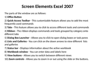
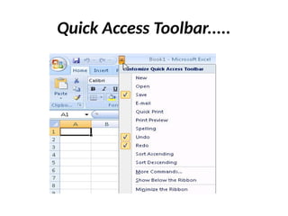
Screen Elements Excel2007
The parts of the window are as follows:
1) Office Button
2) Quick Access Toolbar - This customizable feature allows you to add the most
frequently used commands
3) Tabs - This feature allows you to click to access different tools and commands
4) Ribbon - The ribbon displays commands and tools grouped by category onto
different tabs
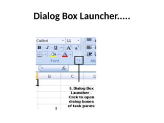
5) Dialog Box Launcher - Allows you to click to open dialog boxes or task panes
6) Lists and Galleries - You can click on the down arrows to view different lists
and galleries
7) Status bar - Displays information about the active workbook
8) Workbook window - You can enter data and labels here
9) View buttons - Allows you to switch between different views
10) Zoom controls - Allows you to zoom in or out using the slide or the buttons.
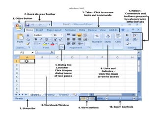
Office Button
• InMicrosoft Excel 2007, the Office button is
located in the upper-left hand corner of the
window. This button allows access to different
file commands such as New, Open, Save, Save
As, and Print. It performs the same function as
the File Menu.
9.
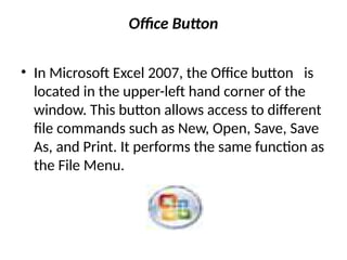
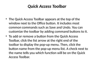
Quick Access Toolbar
•The Quick Access Toolbar appears at the top of the
window next to the Office button. It includes most
common commands such as Save and Undo. You can
customize the toolbar by adding command buttons to it.
• To add or remove a button from the Quick Access
Toolbar, click the list arrow at the right end of the
toolbar to display the pop-up menu. Then, click the
button name from the pop-up menu list. A check next to
the name tells you which function will be on the Quick
Access Toolbar.
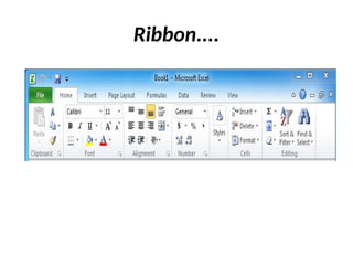
Ribbon
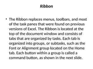
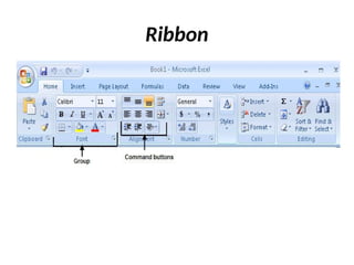
• The Ribbonreplaces menus, toolbars, and most
of the task panes that were found on previous
versions of Excel. The Ribbon is located at the
top of the document window and consists of
tabs that are organized by tasks. Each tab is
organized into groups, or subtasks, such as the
Font or Alignment group located on the Home
tab. Each button within a group is called a
command button, as shown in the next slide.
Tabs
Excel 2007 providesthree types of tabs on the Ribbon:
• The first are called Standard tabs, which are the default tabs that
appear when you start Microsoft Word. They include Home,
Insert, Page Layout, Formulas, Data, Review, View, and Add-Ins
(optional).
• The second are called Contextual tabs, such as Picture Tools,
Drawing, or Table, that appear only when performing a certain
task. Excel 2007 provides the right set of contextual tabs when
performing certain tasks.
• The third type is called Program tabs tab replace the standard
set of tabs when you switch to certain view modes, such as Print
Preview.
14.
Dialog Box Launcher
•Some groups within Excel 2007 have a Dialog
Box Launcher that is located on the bottom
right-hand corner of each group. Clicking on
the Dialog Box Launcher will open dialog
boxes or task panes that will allow you to
modify the current settings.
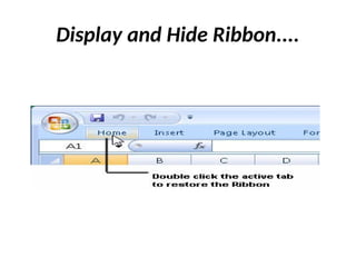
Display and HideRibbon
• In Excel 2007, to minimize the Ribbon double-
click the Home tab.
• You can auto display the Ribbon by clicking
once on the tab, but it will remain minimized
until you double-click the tab again.
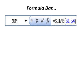
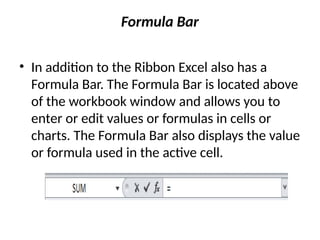
Formula Bar
• Inaddition to the Ribbon Excel also has a
Formula Bar.
• The Formula Bar is located above of the
workbook window and allows you to enter or
edit values or formulas in cells or charts. The
Formula Bar also displays the value or formula
used in the active cell.
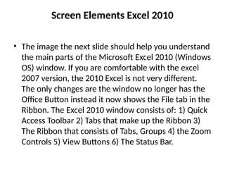
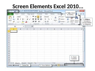
Screen Elements Excel2010
• The image the next slide should help you understand
the main parts of the Microsoft Excel 2010 (Windows
OS) window. If you are comfortable with the excel
2007 version, the 2010 Excel is not very different.
The only changes are the window no longer has the
Office Button instead it now shows the File tab in the
Ribbon. The Excel 2010 window consists of: 1) Quick
Access Toolbar 2) Tabs that make up the Ribbon 3)
The Ribbon that consists of Tabs, Groups 4) the Zoom
Controls 5) View Buttons 6) The Status Bar.
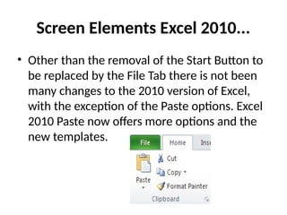
Screen Elements Excel2010...
• Other than the removal of the Start Button to
be replaced by the File Tab there is not been
many changes to the 2010 version of Excel,
with the exception of the Paste options. Excel
2010 Paste now offers more options and the
new templates.
23.
Quick Access Toolbar
•The Quick Access Toolbar appears at the top of the
window next to the Office button. It includes most
common commands such as Save and Undo. You can
customize the toolbar by adding command buttons to it.
• To add or remove a button from the Quick Access
Toolbar, click the list arrow at the right end of the
toolbar to display the pop-up menu. Then, click the
button name from the pop-up menu list. A check next to
the name tells you which function will be on the Quick
Access Toolbar.
24.
Ribbon
• The Ribbonreplaces menus, toolbars, and most
of the task panes that were found on previous
versions of Excel. The Ribbon is located at the
top of the document window and consists of
tabs that are organized by tasks. Each tab is
organized into groups, or subtasks, such as the
Font or Alignment group located on the Home
tab. Each button within a group is called a
command button, as shown the next slide.
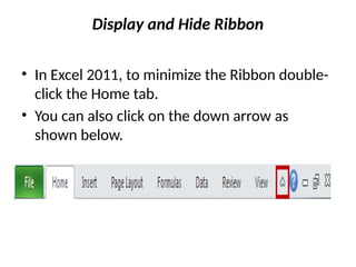
Display and HideRibbon
• In Excel 2011, to minimize the Ribbon double-
click the Home tab.
• You can also click on the down arrow as
shown below.
27.
Formula Bar
• Inaddition to the Ribbon Excel also has a
Formula Bar. The Formula Bar is located above
of the workbook window and allows you to
enter or edit values or formulas in cells or
charts. The Formula Bar also displays the value
or formula used in the active cell.
28.
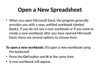
Open a NewSpreadsheet
• When you open Microsoft Excel, the program generally
provides you with a new, untitled workbook labeled
Book1. If you do not see a new workbook or if you want to
create a new workbook after you have opened Microsoft
Excel, there are several options to choose from.
To open a new workbook: (To open a new workbook using
the keyboard)
• Press the Ctrl button and N at the same time
• A new workbook will appear.
29.
Open a NewSpreadsheet...
• After you have opened a new workbook,
notice there will be a default title at the top of
the page ex. Book1. It is recommended you
save your workbook now with a unique name
before you begin working within the
workbook. Refer to the section later in this
module called Saving a Workbook for more
information.
30.
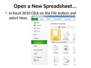
Open a NewSpreadsheet...
• In Excel 2010 Click on the File button and
select New.
31.
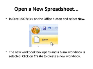
Open a NewSpreadsheet...
• In Excel 2007click on the Office button and select New.
• The new workbook box opens and a blank workbook is
selected. Click on Create to create a new workbook.
32.
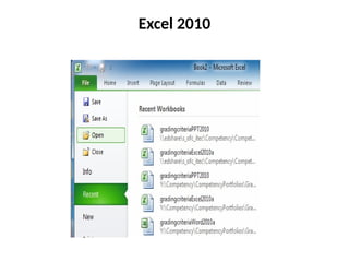
Open an ExistingWorkbook
• To open an existing workbook in Excel 2010, if
the workbook you want to open was used
recently you can go to the File Menu and click
Recent and select the file you wan to open. If
the file was not recently used click Open.
Open Dialog box will open and select the file
from where it was last saved.
Excel 2007
• Toopen an existing workbook in Excel 2007, if
the workbook you want to open is one that
was used recently, it will be listed under the
Office button and the recently used files will
be listed. Select the file and it will open
automatically. If the file came from a
removable disk be sure to insert the disk into
the corresponding drive in order to retrieve
the file.
35.
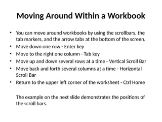
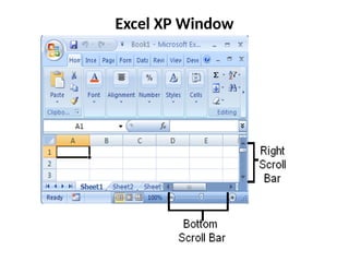
Moving Around Withina Workbook
• You can move around workbooks by using the scrollbars, the
tab markers, and the arrow tabs at the bottom of the screen.
• Move down one row - Enter key
• Move to the right one column - Tab key
• Move up and down several rows at a time - Vertical Scroll Bar
• Move back and forth several columns at a time - Horizontal
Scroll Bar
• Return to the upper left corner of the worksheet - Ctrl Home
The example on the next slide demonstrates the positions of
the scroll bars.
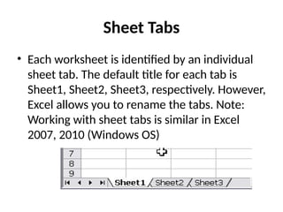
Sheet Tabs
• Eachworksheet is identified by an individual
sheet tab. The default title for each tab is
Sheet1, Sheet2, Sheet3, respectively. However,
Excel allows you to rename the tabs. Note:
Working with sheet tabs is similar in Excel
2007, 2010 (Windows OS)
38.
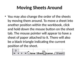
Moving Sheets Around
•You may also change the order of the sheets
by moving them around. To move a sheet into
another position within the workbook, click
and hold down the mouse button on the sheet
tab. The mouse pointer will appear to have a
sheet of paper attached to it. There will also
be a black triangle indicating the current
position of the sheet.
39.
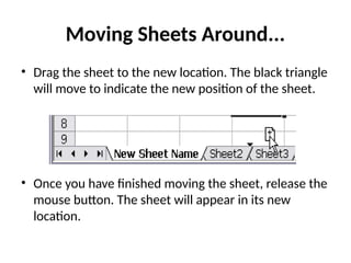
Moving Sheets Around...
•Drag the sheet to the new location. The black triangle
will move to indicate the new position of the sheet.
• Once you have finished moving the sheet, release the
mouse button. The sheet will appear in its new
location.
40.
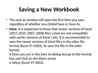
Saving a NewWorkbook
• The save as window will open the first time you save
regardless of whether you clicked Save or Save As.
• Note: It is important to know that newer versions of Excel
(2011,2010, 2007, 2008) files (.xlsx) are not compatible
with earlier versions of Excel (.xls). It is recommended to
save the newer versions of Excel files in the older file
format (Excel 97-2003). To save the file in the older
format:
• Once you are in the Save As dialog box go to the Format
box and click on the down arrow.
• Select (Excel 97-2003).
41.
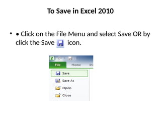
To Save inExcel 2010
• • Click on the File Menu and select Save OR by
click the Save icon.
42.
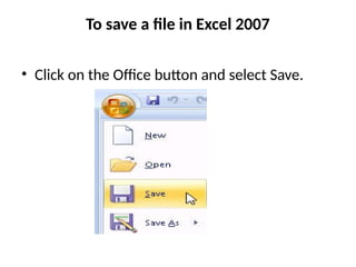
To save afile in Excel 2007
• Click on the Office button and select Save.
43.
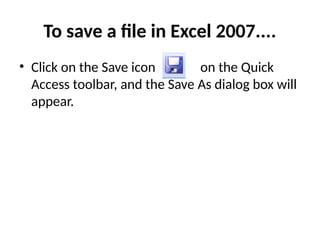
To save afile in Excel 2007....
• Click on the Save icon on the Quick
Access toolbar, and the Save As dialog box will
appear.
44.
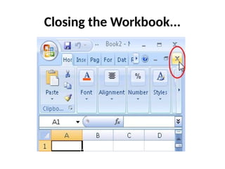
Closing the Workbook
•In Excel 2007 under the Office button click on
the Close command when you want to close a
file without exiting Excel. In Excel 2010 click on
the File tab and select close. Another option
for closing the workbook is to click on the
close box on the workbook window.
Entering Data
• Thislesson will help show you how to enter
data into a spreadsheet.
• Entering data into a spreadsheet is similar in
Excel 2007 and 2010 (Windows OS)
47.
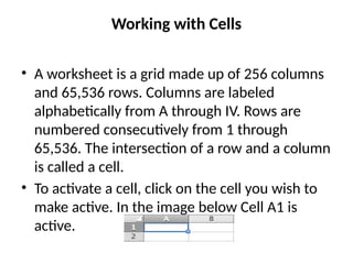
Working with Cells
•A worksheet is a grid made up of 256 columns
and 65,536 rows. Columns are labeled
alphabetically from A through IV. Rows are
numbered consecutively from 1 through
65,536. The intersection of a row and a column
is called a cell.
• To activate a cell, click on the cell you wish to
make active. In the image below Cell A1 is
active.
48.
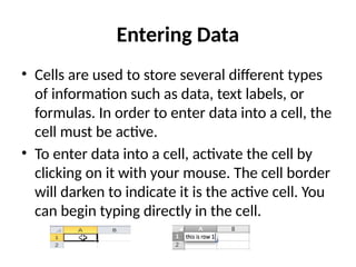
Entering Data
• Cellsare used to store several different types
of information such as data, text labels, or
formulas. In order to enter data into a cell, the
cell must be active.
• To enter data into a cell, activate the cell by
clicking on it with your mouse. The cell border
will darken to indicate it is the active cell. You
can begin typing directly in the cell.
49.
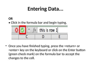
Entering Data...
OR
• Clickin the formula bar and begin typing.
• Once you have finished typing, press the <return> or
<enter> key on the keyboard or click on the Enter button
(green check mark) on the formula bar to accept the
changes to the cell.
50.
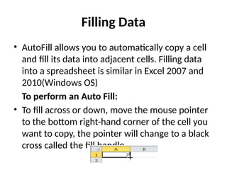
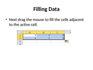
Filling Data
• AutoFillallows you to automatically copy a cell
and fill its data into adjacent cells. Filling data
into a spreadsheet is similar in Excel 2007 and
2010(Windows OS)
To perform an Auto Fill:
• To fill across or down, move the mouse pointer
to the bottom right-hand corner of the cell you
want to copy, the pointer will change to a black
cross called the fill handle.
51.
Filling Data
• Nextdrag the mouse to fill the cells adjacent
to the active cell.
52.
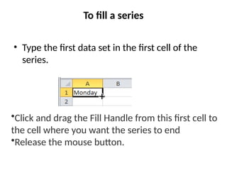
To fill aseries
• Type the first data set in the first cell of the
series.
•Click and drag the Fill Handle from this first cell to
the cell where you want the series to end.
•Release the mouse button.
53.
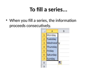
To fill aseries...
• When you fill a series, the information
proceeds consecutively.
54.
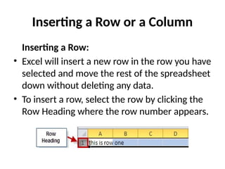
Inserting a Rowor a Column
Inserting a Row:
• Excel will insert a new row in the row you have
selected and move the rest of the spreadsheet
down without deleting any data.
• To insert a row, select the row by clicking the
Row Heading where the row number appears.
55.
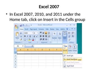
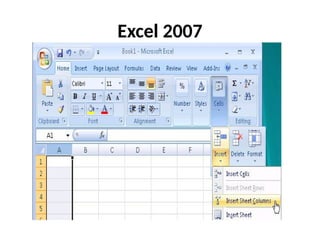
Excel 2007
• InExcel 2007, 2010, and 2011 under the
Home tab, click on Insert in the Cells group
56.
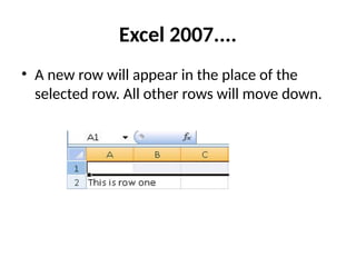
Excel 2007....
• Anew row will appear in the place of the
selected row. All other rows will move down.
57.
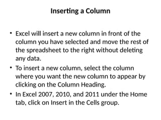
Inserting a Column
•Excel will insert a new column in front of the
column you have selected and move the rest of
the spreadsheet to the right without deleting
any data.
• To insert a new column, select the column
where you want the new column to appear by
clicking on the Column Heading.
• In Excel 2007, 2010, and 2011 under the Home
tab, click on Insert in the Cells group.
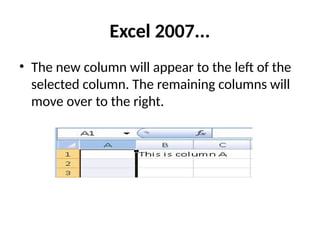
Excel 2007...
• Thenew column will appear to the left of the
selected column. The remaining columns will
move over to the right.
60.
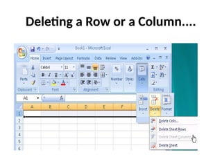
Deleting a Rowor a Column
• To delete a row or column, select the row or
column you wish to delete.
• In Excel 2007, 2010, and 2011 under the
Home tab select Delete under the Cells group.
Then, select Delete Sheet rows or columns.
Deleting a Rowor a Column....
OR
• Right click over the row or column header and
select delete from the contextual menu.
63.
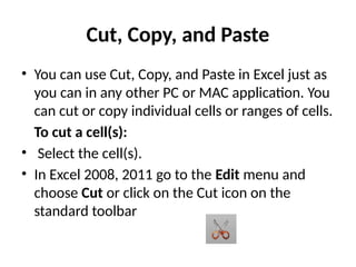
Cut, Copy, andPaste
• You can use Cut, Copy, and Paste in Excel just as
you can in any other PC or MAC application. You
can cut or copy individual cells or ranges of cells.
To cut a cell(s):
• Select the cell(s).
• In Excel 2008, 2011 go to the Edit menu and
choose Cut or click on the Cut icon on the
standard toolbar
64.
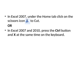
• In Excel2007, under the Home tab click on the
scissors icon to Cut.
OR
• In Excel 2007 and 2010, press the Ctrl button
and X at the same time on the keyboard.
65.
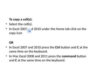
To copy acell(s):
• Select the cell(s).
• In Excel 2007 and 2010 under the Home tab click on the
copy icon
OR
• In Excel 2007 and 2010 press the Ctrl button and C at the
same time on the keyboard.
• In Mac Excel 2008 and 2011 press the command button
and C at the same time on the keyboard.
66.
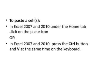
• To pastea cell(s):
• In Excel 2007 and 2010 under the Home tab
click on the paste icon
OR
• In Excel 2007 and 2010, press the Ctrl button
and V at the same time on the keyboard.
67.
Formulas
• In thislesson you will learn how to perform
calculations in the spreadsheet using
formulas. A formula is a sequence of values,
cell references and operators used to produce
a new value from existing cells.
68.
Parts of aFormula
• Formulas are used to perform calculations.
Excel formulas always begin with an equal
sign, which tells Excel that you have entered a
formula rather than a number or text.
• Example: =A1+A2 (gives the sum of the values
in these two cells)
69.
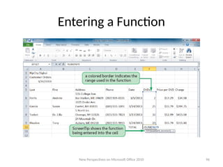
Entering a Formula
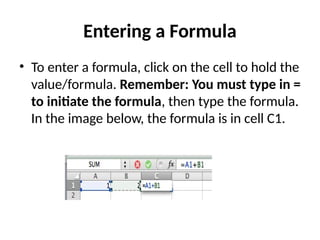
•To enter a formula, click on the cell to hold the
value/formula. Remember: You must type in =
to initiate the formula, then type the formula.
In the image below, the formula is in cell C1.
70.
Entering a Formula...
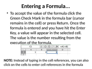
•To accept the value of the formula click the
Green Check Mark in the formula bar (cursor
remains in the cell) or press Return. Once the
formula is entered and you have hit the Enter
Key, a value will appear in the selected cell.
The value is the number resulting from the
execution of the formula.
NOTE: Instead of typing in the cell references, you can also
click on the cells to enter cell references in the formula
71.
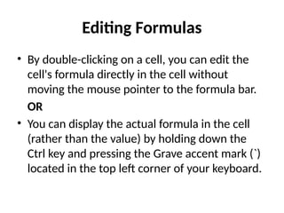
Editing Formulas
• Bydouble-clicking on a cell, you can edit the
cell's formula directly in the cell without
moving the mouse pointer to the formula bar.
OR
• You can display the actual formula in the cell
(rather than the value) by holding down the
Ctrl key and pressing the Grave accent mark (`)
located in the top left corner of your keyboard.
72.
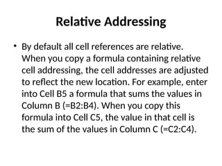
Relative Addressing
• Bydefault all cell references are relative.
When you copy a formula containing relative
cell addressing, the cell addresses are adjusted
to reflect the new location. For example, enter
into Cell B5 a formula that sums the values in
Column B (=B2:B4). When you copy this
formula into Cell C5, the value in that cell is
the sum of the values in Column C (=C2:C4).
73.
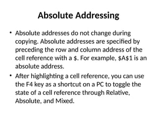
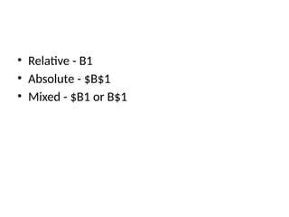
Absolute Addressing
• Absoluteaddresses do not change during
copying. Absolute addresses are specified by
preceding the row and column address of the
cell reference with a $. For example, $A$1 is an
absolute address.
• After highlighting a cell reference, you can use
the F4 key as a shortcut on a PC to toggle the
state of a cell reference through Relative,
Absolute, and Mixed.
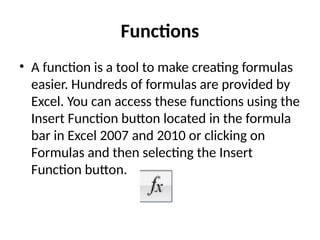
Functions
• A functionis a tool to make creating formulas
easier. Hundreds of formulas are provided by
Excel. You can access these functions using the
Insert Function button located in the formula
bar in Excel 2007 and 2010 or clicking on
Formulas and then selecting the Insert
Function button.
76.
To create afunction in Excel 2007 and 2010:
• To create a function using the Insert Function
button, first activate the cell where you would
like to insert the function.
• Next, click on the Insert Function button.
• The Insert Function dialog box appears.
77.
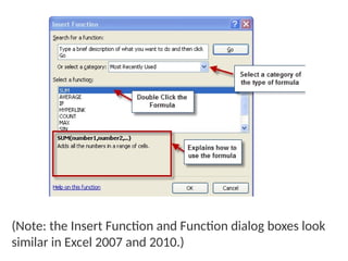
(Note: the InsertFunction and Function dialog boxes look
similar in Excel 2007 and 2010.)
78.
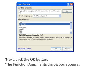
The example inthe next slide demonstrates how to
use the Average Function.
• First, select the cell where the formula will be
placed.
• Then click on the Insert Function button.
• The Insert Function dialog box will appear. From the
Select a function: menu, choose the appropriate
function. An explanation of the chosen formula
appears at the bottom of the dialog box.
79.
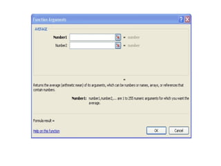
•Next, click theOK button.
•The Function Arguments dialog box appears.
81.
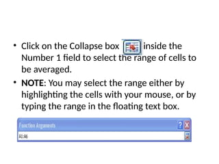
• Click onthe Collapse box inside the
Number 1 field to select the range of cells to
be averaged.
• NOTE: You may select the range either by
highlighting the cells with your mouse, or by
typing the range in the floating text box.
82.
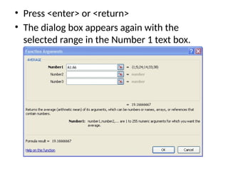
• Press <enter>or <return>
• The dialog box appears again with the
selected range in the Number 1 text box.
83.
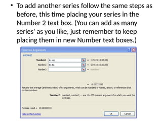
• To addanother series follow the same steps as
before, this time placing your series in the
Number 2 text box. (You can add as many
series' as you like, just remember to keep
placing them in new Number text boxes.)
84.
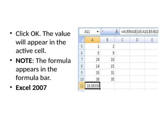
• Click OK.The value
will appear in the
active cell.
• NOTE: The formula
appears in the
formula bar.
• Excel 2007
85.
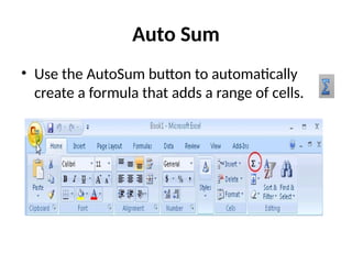
Auto Sum
• Usethe AutoSum button to automatically
create a formula that adds a range of cells.
86.
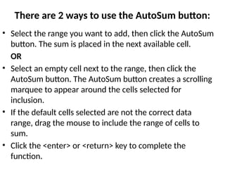
There are 2ways to use the AutoSum button:
• Select the range you want to add, then click the AutoSum
button. The sum is placed in the next available cell.
OR
• Select an empty cell next to the range, then click the
AutoSum button. The AutoSum button creates a scrolling
marquee to appear around the cells selected for
inclusion.
• If the default cells selected are not the correct data
range, drag the mouse to include the range of cells to
sum.
• Click the <enter> or <return> key to complete the
function.
87.
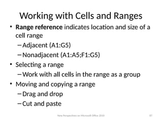
Working with Cellsand Ranges
• Range reference indicates location and size of a
cell range
–Adjacent (A1:G5)
–Nonadjacent (A1:A5;F1:G5)
• Selecting a range
–Work with all cells in the range as a group
• Moving and copying a range
–Drag and drop
–Cut and paste
New Perspectives on Microsoft Office 2010 87
88.
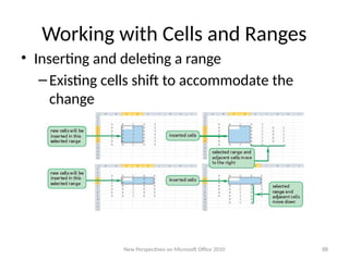
Working with Cellsand Ranges
• Inserting and deleting a range
–Existing cells shift to accommodate the
change
New Perspectives on Microsoft Office 2010 88
89.
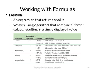
Working with Formulas
•Formula
– An expression that returns a value
– Written using operators that combine different
values, resulting in a single displayed value
New Perspectives on Microsoft Office 2010 89
90.
Working with Formulas
•Entering a formula
–Click cell where you want formula results to
appear
–Type = and an expression that calculates a value
using cell references and arithmetic operators
• Cell references allow you to change values
used in the calculation without having to
modify the formula itself
–Press Enter or Tab to complete the formula
New Perspectives on Microsoft Office 2010 90
91.
Working with Formulas
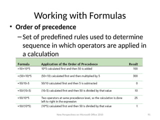
•Order of precedence
–Set of predefined rules used to determine
sequence in which operators are applied in
a calculation
New Perspectives on Microsoft Office 2010 91
92.
Working with Formulas
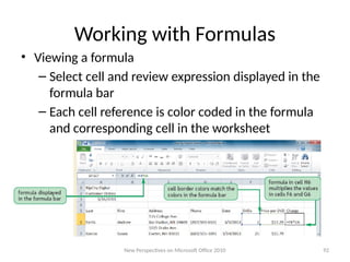
•Viewing a formula
– Select cell and review expression displayed in the
formula bar
– Each cell reference is color coded in the formula
and corresponding cell in the worksheet
New Perspectives on Microsoft Office 2010 92
93.
Working with Formulas
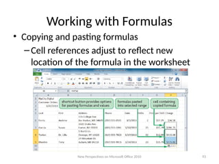
•Copying and pasting formulas
–Cell references adjust to reflect new
location of the formula in the worksheet
New Perspectives on Microsoft Office 2010 93
94.
Working with Formulas
•Guidelines for writing effective formulas:
–Keep them simple
–Do not hide data values within formulas
–Break up formulas to show intermediate
results
New Perspectives on Microsoft Office 2010 94
95.
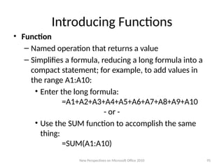
Introducing Functions
• Function
–Named operation that returns a value
– Simplifies a formula, reducing a long formula into a
compact statement; for example, to add values in
the range A1:A10:
• Enter the long formula:
=A1+A2+A3+A4+A5+A6+A7+A8+A9+A10
- or -
• Use the SUM function to accomplish the same
thing:
=SUM(A1:A10)
New Perspectives on Microsoft Office 2010 95
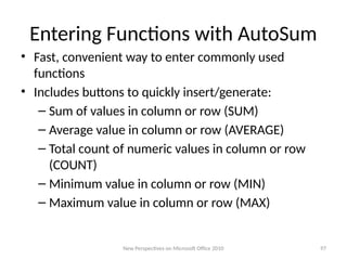
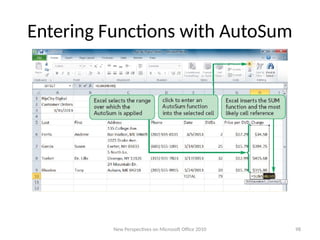
Entering Functions withAutoSum
• Fast, convenient way to enter commonly used
functions
• Includes buttons to quickly insert/generate:
– Sum of values in column or row (SUM)
– Average value in column or row (AVERAGE)
– Total count of numeric values in column or row
(COUNT)
– Minimum value in column or row (MIN)
– Maximum value in column or row (MAX)
New Perspectives on Microsoft Office 2010 97
Working with Worksheets
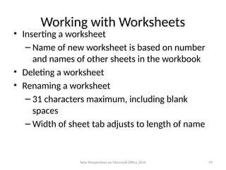
•Inserting a worksheet
– Name of new worksheet is based on number
and names of other sheets in the workbook
• Deleting a worksheet
• Renaming a worksheet
– 31 characters maximum, including blank
spaces
– Width of sheet tab adjusts to length of name
New Perspectives on Microsoft Office 2010 99
100.
Working with Worksheets
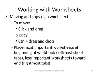
•Moving and copying a worksheet
–To move:
• Click and drag
–To copy:
• Ctrl + drag and drop
–Place most important worksheets at
beginning of workbook (leftmost sheet
tabs), less important worksheets toward
end (rightmost tabs)
New Perspectives on Microsoft Office 2010 100
101.
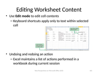
Editing Worksheet Content
•Use Edit mode to edit cell contents
– Keyboard shortcuts apply only to text within selected
cell
• Undoing and redoing an action
– Excel maintains a list of actions performed in a
workbook during current session
New Perspectives on Microsoft Office 2010 101
102.
Formatting Text
• Youcan format cells to change the way the text appears
in a cell. You can change the font type, size, and style
(bold, italics, underlined). In addition, you can also add
special effects such as wrapping the text in a cell and
having text merge in a selected number of cells. Since
font changes are associated with the cell and not the
contents, you can change the font before or after you
enter information.
• In Excel 2007, 2010, and 2011 under the Home tab you
can use the groups to format the text within a cell or
group of cells.
103.
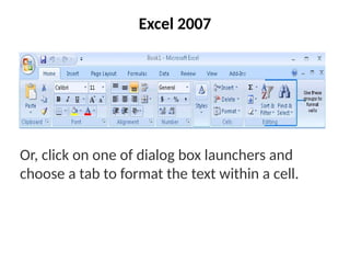
Excel 2007
Or, clickon one of dialog box launchers and
choose a tab to format the text within a cell.
104.
Formatting Numbers
• InExcel 2007, 2010, 2011 formatting may be
accessed under the Home tab and using the
different groups such as, Font, Alignment,
Number, Styles, Cells, and Editing. To format
numbers you can also access the dialog box
launcher under on the bottom right hand side
of the Number group to allow for more
formatting.
105.
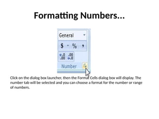
Formatting Numbers...
Click onthe dialog box launcher, then the Format Cells dialog box will display. The
number tab will be selected and you can choose a format for the number or range
of numbers.
106.
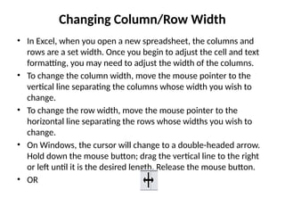
Changing Column/Row Width
•In Excel, when you open a new spreadsheet, the columns and
rows are a set width. Once you begin to adjust the cell and text
formatting, you may need to adjust the width of the columns.
• To change the column width, move the mouse pointer to the
vertical line separating the columns whose width you wish to
change.
• To change the row width, move the mouse pointer to the
horizontal line separating the rows whose widths you wish to
change.
• On Windows, the cursor will change to a double-headed arrow.
Hold down the mouse button; drag the vertical line to the right
or left until it is the desired length. Release the mouse button.
• OR
107.
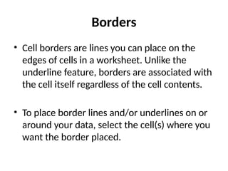
Borders
• Cell bordersare lines you can place on the
edges of cells in a worksheet. Unlike the
underline feature, borders are associated with
the cell itself regardless of the cell contents.
• To place border lines and/or underlines on or
around your data, select the cell(s) where you
want the border placed.
108.
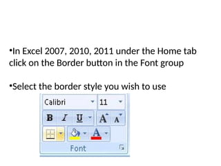
•In Excel 2007,2010, 2011 under the Home tab
click on the Border button in the Font group
•Select the border style you wish to use
109.
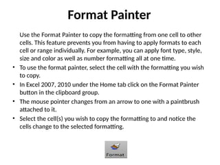
Format Painter
Use theFormat Painter to copy the formatting from one cell to other
cells. This feature prevents you from having to apply formats to each
cell or range individually. For example, you can apply font type, style,
size and color as well as number formatting all at one time.
• To use the format painter, select the cell with the formatting you wish
to copy.
• In Excel 2007, 2010 under the Home tab click on the Format Painter
button in the clipboard group.
• The mouse pointer changes from an arrow to one with a paintbrush
attached to it.
• Select the cell(s) you wish to copy the formatting to and notice the
cells change to the selected formatting.
110.
Creating Charts
• Inthis lesson, you will learn how to create
charts using the data in your workbook. A
chart is a graphic representation of worksheet
data. Charts are useful when explaining the
data in your spreadsheet in a presentational
way
111.
Types of Charts
•Excel has several different types of charts to
choose from. Some charts are better than
others for presenting certain types of
information. This lesson will introduce four of
the most frequently used chart types and their
functions.
112.
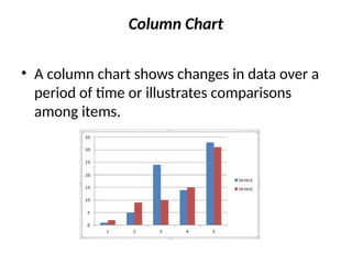
Column Chart
• Acolumn chart shows changes in data over a
period of time or illustrates comparisons
among items.
113.
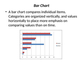
Bar Chart
• Abar chart compares individual items.
Categories are organized vertically, and values
horizontally to place more emphasis on
comparing values than on time.
114.
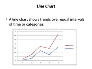
Line Chart
• Aline chart shows trends over equal intervals
of time or categories.
115.
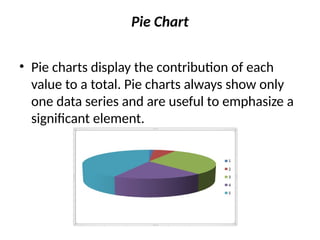
Pie Chart
• Piecharts display the contribution of each
value to a total. Pie charts always show only
one data series and are useful to emphasize a
significant element.
116.
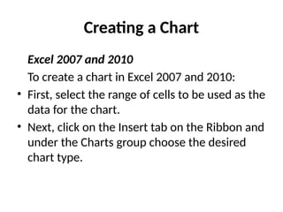
Creating a Chart
Excel2007 and 2010
To create a chart in Excel 2007 and 2010:
• First, select the range of cells to be used as the
data for the chart.
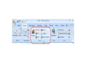
• Next, click on the Insert tab on the Ribbon and
under the Charts group choose the desired
chart type.
118.
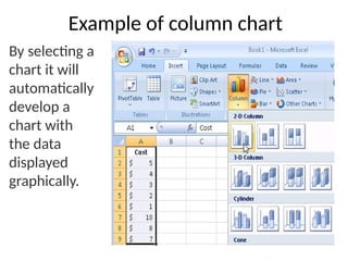
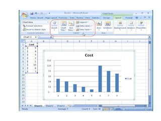
Example of columnchart
By selecting a
chart it will
automatically
develop a
chart with
the data
displayed
graphically.
120.
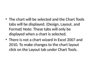
• The chartwill be selected and the Chart Tools
tabs will be displayed. (Design, Layout, and
Format) Note: These tabs will only be
displayed when a chart is selected.
• There is not a chart wizard in Excel 2007 and
2010. To make changes to the chart layout
click on the Layout tab under Chart Tools.
121.
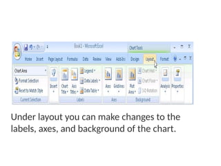
Under layout youcan make changes to the
labels, axes, and background of the chart.
122.
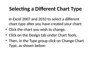
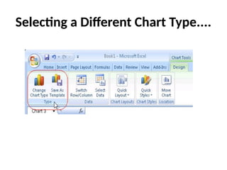
Selecting a DifferentChart Type
In Excel 2007 and 2010 to select a different
chart type after you have created your chart:
• Click the chart you wish to change.
• Click on the Design tab under Chart Tools.
• Then, in the Type group click on Change Chart
Type, as shown below:
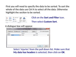
Select ‘injuries’ fromthe pull down list. Make sure that
My data has headers is selected, then click on OK.
A dialogue box will appear.
Click on the Sort and Filter icon.
Then select Custom Sort.
First you will need to specify the data to be sorted. To sort the
whole of the data use Ctrl A to select all the data. Otherwise
highlight the section to be sorted.
125.
Exercise
• Create astudent records consisting of five
subjects and about twenty students. The
student records should have the sum, average
and grade of each student
• Then create a chart showing the name of
students and average marks only (just two
column in the graph)