Section 3 f.ppt

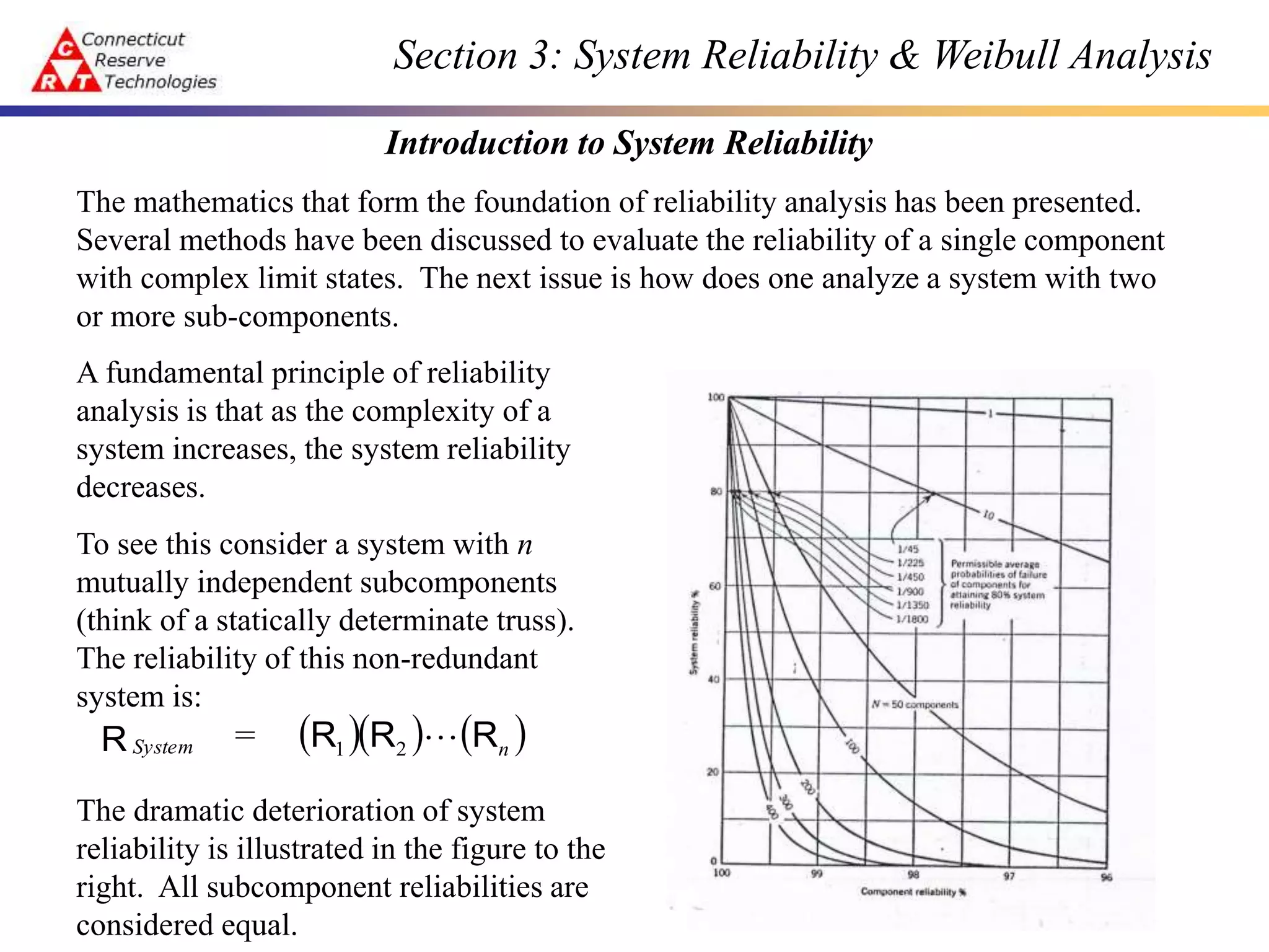
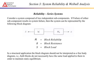
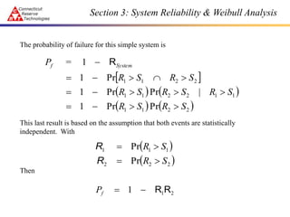
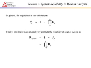
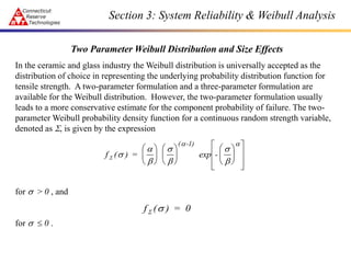
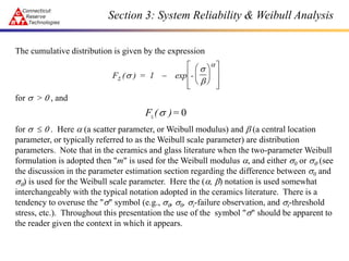
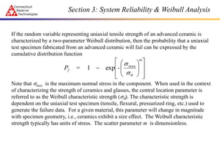
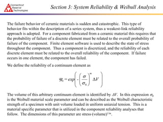
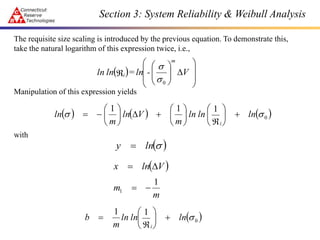
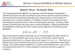
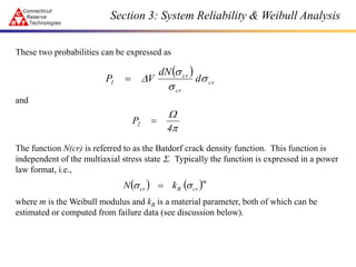
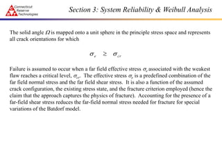
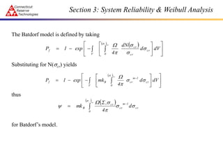
Section 3: System Reliability & Weibull Analysis
Introduction to System Reliability
The mathematics that form the foundation of reliability analysis has been presented.
Several methods have been discussed to evaluate the reliability of a single component
with complex limit states. The next issue is how does one analyze a system with two
or more sub-components.
A fundamental principle of reliability
analysis is that as the complexity of a
system increases, the system reliability
decreases.
To see this consider a system with n
mutually independent subcomponents
(think of a statically determinate truss).
The reliability of this non-redundant
system is:
The dramatic deterioration of system
reliability is illustrated in the figure to the
right. All subcomponent reliabilities are
considered equal.
    
n
System = R
R
R
R 
2
1

There are three basic categories of systems based on how the overall reliability is
computed. They are
1. Series Systems (example just presented)
2. Parallel Systems (indeterminate trusses, composite material systems)
3. Systems with active redundancies (r out of n systems)
The brittle failure behavior of ceramic materials is best modeled by a series system. The
next section provides the motivation for the expression found on the previous overhead.

Reliability – Series Systems
Consider a system composed of two independent sub-components. If Failure of either
sub-component results in system failure, then the system can be represented by the
following block diagram:
In a structural application the block diagram should not be interpreted as a free body
diagram, i.e., both blocks do not necessarily have the same load applied to them in
order to maintain static equilibrium.
Load
Block
S
Resistance
Block
R
y
Reliabilit
Block



R

The probability of failure for this simple system is
This last result is based on the assumption that both events are statistically
independent. With
Then
 
   
   
2
2
1
1
1
1
2
2
1
1
2
2
1
1
Pr
Pr
1
|
Pr
Pr
1
Pr
1
1
S
R
S
R
S
R
S
R
S
R
S
R
S
R
=
P System
f














 R
 
 
2
2
2
1
1
1
Pr
Pr
S
R
S
R




R
R
2
1
1 R
R


f
P

In general, for a system on n sub-components
Finally, note that we can alternatively compute the reliability of a series system as




n
R
1
1
i
i
f
P





n
R
R
1
1
i
i
f
System P

Series System Example – Statically Determinate Truss
(overheads)

Two Parameter Weibull Distribution and Size Effects
In the ceramic and glass industry the Weibull distribution is universally accepted as the
distribution of choice in representing the underlying probability distribution function for
tensile strength. A two-parameter formulation and a three-parameter formulation are
available for the Weibull distribution. However, the two-parameter formulation usually
leads to a more conservative estimate for the component probability of failure. The two-
parameter Weibull probability density function for a continuous random strength variable,
denoted as S, is given by the expression
for s > 0 , and
for s  0 .
f ( ) = -
( -1)
S s


s

s

 


























exp
f ( ) =
S s 0

The cumulative distribution is given by the expression
for s > 0 , and
for s  0 . Here  (a scatter parameter, or Weibull modulus) and  (a central location
parameter, or typically referred to as the Weibull scale parameter) are distribution
parameters. Note that in the ceramics and glass literature when the two-parameter Weibull
formulation is adopted then "m" is used for the Weibull modulus , and either s0 or sq (see
the discussion in the parameter estimation section regarding the difference between s0 and
sq) is used for the Weibull scale parameter. Here the (, ) notation is used somewhat
interchangeably with the typical notation adopted in the ceramics literature. There is a
tendency to overuse the "s" symbol (e.g., sq, s0, si-failure observation, and st-threshold
stress, etc.). Throughout this presentation the use of the symbol "s" should be apparent to
the reader given the context in which it appears.
F ( ) = -
S s
s


1 














exp
0
=
)
(
F s
S

If the random variable representing uniaxial tensile strength of an advanced ceramic is
characterized by a two-parameter Weibull distribution, then the probability that a uniaxial
test specimen fabricated from an advanced ceramic will fail can be expressed by the
cumulative distribution function
Note that smax is the maximum normal stress in the component. When used in the context
of characterizing the strength of ceramics and glasses, the central location parameter is
referred to as the Weibull characteristic strength (sq). The characteristic strength is
dependent on the uniaxial test specimen (tensile, flexural, pressurized ring, etc.) used to
generate the failure data. For a given material, this parameter will change in magnitude
with specimen geometry, i.e., ceramics exhibit a size effect. The Weibull characteristic
strength typically has units of stress. The scatter parameter m is dimensionless.

















q
s
smax
exp
1
m
f -
=
P

Ceramic materials typically exhibit rather high tensile strength with a relatively low
fracture toughness (typically quantified by KIC). Lack of ductility (i.e., lack of fracture
toughness) leads to low strain tolerance and large variations in observed fracture
strength. When a load is applied, the absence of significant plastic deformation or
micro-cracking causes large stress concentrations to occur at microscopic flaws. These
flaws are unavoidably present as a result of fabrication or in-service environmental
factors.
To date non-destructive evaluation (NDE) inspection programs with sufficient
resolution have not been successfully implemented into fabrication operations. The
combination of high strength and low fracture toughness leads to relatively small
critical defect sizes that can not be detected by current NDE methods. As a result,
components with a distribution of defects (characterized by various crack sizes and
orientations) are produced which leads to an observed scatter in component tensile
strength. The distribution of defects leads to an apparent decrease in tensile strength as
the size of the component increases. This is the so-called strength-size effect, i.e., with
bigger components there is an increased chance that larger more deleterious flaws are
present. Design methods for ceramic components must admit size dependence. This is
accomplished through the use of reliability concepts where the component is treated as
a system, and the probability of failure of the system must be ascertained.

The failure behavior of ceramic materials is sudden and catastrophic. This type of
behavior fits within the description of a series system, thus a weakest-link reliability
approach is adopted. For a component fabricated from a ceramic material this requires that
the probability of failure of a discrete element must be related to the overall probability of
failure of the component. Finite element software is used to describe the state of stress
throughout the component. Thus a component is discretized, and the reliability of each
discrete element must be related to the overall reliability of the component. If failure
occurs in one element, the component has failed.
We define the reliability of a continuum element as
The volume of this arbitrary continuum element is identified by V. In this expression s0
is the Weibull material scale parameter and can be described as the Weibull characteristic
strength of a specimen with unit volume loaded in uniform uniaxial tension. This is a
material specific parameter that is utilized in the component reliability analyses that
follow. The dimensions of this parameter are stress(volume)1/m.

















 V
-
exp
=
m
i
0
s
s

The requisite size scaling is introduced by the previous equation. To demonstrate this,
take the natural logarithm of this expression twice, i.e.,
Manipulation of this expression yields
with
  
















 V
-
ln
=
ln
ln
m
i
0
s
s
     
0
1
1
1
s
s ln
ln
ln
m
V
ln
m
ln
i
























 
s
ln
y 
 
V
ln
x 

m
m
1
1 

 
0
1
1
s
ln
ln
ln
m
b
i










then it is apparent that the double log equation has the form of a straight line, i.e.,
y = m1x + b, and plots as follows.
Consider several groups of test specimens fabricated from the same material. The
specimens in each group are identical with each other, but the two groups have different
gage sections such that V (which is now identified as the gage section volume; or A which
is identified as the gage area) is different for each group of specimens. Estimate Weibull
parameters m and s0 from the pooled failure data obtained from each group (parameter
estimation and pooling techniques are discussed in a later section).
 
s
ln
y  m
slope
1


 
V
ln
x 


After the Weibull parameters are estimated the line for y = m1x + b can be plotted that
corresponds to say (i.e., the 50th percentile). This value for should correlate
well with the median values in each group, if the number in each group is large.
%
50

i
Plot this specific curve as a function of
the gage volumes (V) or gage area
(A) for each group, as is done to the
right. If no size effect is present, then
median failure strengths of the groups
will fall close to a horizontal line. This
would indicate no correlation between
gage geometry and the median strength
value. A systematic variation away
from a horizontal line approaching the
curve y = m1x + b indicates that a size
effect is present. The figure to the
right appears in Johnson and Tucker
(1991)

Component Reliability
The ability to account for size effects of individual elements was introduced through the
expression appearing in the previous section, i.e.,
Now a general expression for the probability of failure for a component is derived based.
Under the assumptions that the component consists of an infinite number of elements (i.e.,
the continuum assumption) and that the component is best represented by a series system,
then

















 V
-
exp
=
m
i
0
s
s
f
k i=1
k
i
P = 1 -

 






lim

substitution leads to
The limit inside the bracket is a Riemann sum. Thus
Weibull (1939) first proposed this integral representation for the probability of failure. The
expression is integrated over all tensile regions of the specimen volume if the strength-
controlling flaws are randomly distributed through the volume of the material, or over all
tensile regions of the specimen area if flaws are restricted to the specimen surface. For
failures due to surface defects the probability of failure is given by the expression






























V
lim
-
exp
-
1
=
P
m
i
k
1
=
i
k
f
0
s
s

















  dV
exp
1
=
P
m
f
0
s
s

















  dA
σ
σ
exp
1
=
P
0
m
f

Over the years a number of reliability models have been presented that extend the uniaxial
format of the previous two integral expressions to multiaxial states of stress. Only models
associated with isotropic brittle materials are presented here. Anisotropic reliability
models are beyond the scope of this presentation. The reader can consult the work of
Duffy and co-workers (1990 and 1990) for information pertaining to reliability models for
brittle composites. The monolithic models highlighted here include the principle of
independent action (PIA) model and Batdorf’s model. A brief discussion is presented for
each.

Multiaxial Reliability Models
A number of reliability models have been presented in the literature that assess
component reliability based on multiaxial states of stress. The two monolithic models
highlighted here include the principle of independent action (PIA) model and
Batdorf’s model. A brief discussion is presented for each. In order to simplify the
presentation of each model component probability of failure is expressed in the
following generic format
where y is identified as a failure function per unit volume. What remains is the
specification of the failure function y for each reliability model.
 
dV
1
=
Pf 

 
exp

PIA – A Phenomenological Model
For the principle of independent action (PIA) model:
where s1 , s2 and s3 are the three principal stresses at a given point. Recall that s0 is the
Weibull material scale parameter and can be described as the Weibull characteristic strength
of a specimen with unit volume, or area, loaded in uniform uniaxial tension.
The PIA model is the probabilistic equivalent to the deterministic maximum stress failure
theory. The PIA model has been widely applied in brittle material design. However, the PIA
model does not specify the nature of the defect causing failure. In essence the model is
phenomenological, which does not imply that the model is not useful. The simplicity of
phenomenological models can often times be a strength, not a weakness
m
0
3
m
0
2
m
0
1



























s
s
s
s
s
s


Weibull Analysis – Closed Form Examples
(overheads)

Batdorf’s Theory - Mechanistic Model
The concepts proposed by Batdorf are important in that the approach incorporates a
mechanistic basis for the effect of multiaxial states of stress into the weakest-link theory.
Here material defects distributed throughout the volume (and/or over the surface) are
assumed to have a random orientation. In addition, the defects are assumed to be non-
interacting discontinuities (cracks) with an assumed regular geometry. Consider a finite
volume of material where the stress state is uniform throughout. Batdorf postulated that
the probability of failure for this finite volume can be expressed by the following joint
probability
Here S represents the uniform multiaxial state of stress throughout the finite volume. In
addition, P1 is the probability that a crack exists in V (the finite volume) with an
associated critical stress (i.e., fracture stress) in the range of scr to scr+dcr. Note that scr is
defined as the critical far field normal stress for a given crack configuration under mode I
loading. The second marginal probability, P2, denotes the probability that a crack with an
associated critical stress of scr will be oriented in a direction such that se equals or
exceeds scr.
  2
1
cr
f P
P
=
V
,
,
P 
s
S

These two probabilities can be expressed as
and
The function N(cr) is referred to as the Batdorf crack density function. This function is
independent of the multiaxial stress state S. Typically the function is expressed in a power
law format, i.e.,
where m is the Weibull modulus and kB is a material parameter, both of which can be
estimated or computed from failure data (see discussion below).
 
cr
cr
cr
1 d
dN
V
P s
s
s




4
P2 
   m
cr
B
cr k
N s
s 

The solid angle  is mapped onto a unit sphere in the principle stress space and represents
all crack orientations for which
Failure is assumed to occur when a far field effective stress se associated with the weakest
flaw reaches a critical level, scr. The effective stress se is a predefined combination of the
far field normal stress and the far field shear stress. It is also a function of the assumed
crack configuration, the existing stress state, and the fracture criterion employed (hence the
claim that the approach captures the physics of fracture). Accounting for the presence of a
far-field shear stress reduces the far-field normal stress needed for fracture for special
variations of the Batdorf model.
cr
e s
s 

The Batdorf model is defined by taking
Substituting for N(scr) yields
thus
for Batdorf’s model.
 
 














 
 dV
d
dN
4
exp
1
P
max
e
0
cr
cr
cr
V
f
s
s
s
s


 














 


dV
d
4
mk
exp
1
P
max
e
0
cr
1
m
cr
B
V
f
s
s
s


 
 
cr
1
m
cr
0
cr
B d
4
,
mk
max
e
s
s

s
S


s




The solid angle is defined by the following expression
where  and  are azimuthal angles in the principal stress space, and
if and
if .
 
 

 



s
s

2
0 0
cr
e d
d
sin
,
H
  1
,
H cr
e 
s
s
cr
e s
s 
  0
,
H cr
e 
s
s
cr
e s
s 

This leads to the following expression for the component probability failure
assuming that flaws are distributed uniformly throughout the volume of the component.
A similar development would lead to the following expression for failure due to flaws
spatially distributed along the surface of the component, i.e.,
 
 












   
V
2
0
2
0
m
e
BV
f dV
d
d
sin
,
,
z
,
y
,
x
2
k
exp
1
P V







s

 
  







  
A 0
m
e
BA
f dA
d
sin
,
y
,
x
k
exp
1
P V




s


The crack density coefficient kB that appears in the previous expressions is obtained from
failure data. The methodology for obtaining estimates of the Weibull parameters m and
sq was outlined (refer to the section on maximum likelihood estimators). Once these
quantities are estimated kB can be computed since
However, note that kB is a material specific parameter in much the same manner that s0
(the Weibull material scale parameter) is a material specific parameter. The specimen
geometry incorporated in the expression above is compensated by the fact that sq is also
dependent on specimen geometry. Thus the form of the expression above changes from
specimen type, but the estimated value of sq will also change, and the result is that the
computed value of the crack density coefficient should stay consistent from test
geometry to test geometry for a given material.
)
Geometry
Specimen
,
,
m
(
k
=
k B
B q
s

Numerous authors have discussed the stress distribution around cavities of various types,
under different loading conditions, and proposed numerous criteria to describe impending
fracture. However, several issues must be pointed out:
• No prevailing consensus has emerged regarding a best probabilistic fracture
theory. Most current models predict somewhat similar reliability results, despite the
divergence of initial assumptions.
• Moreover, one must approach the mechanistic models with some caution. The
reliability models based on fracture mechanics incorporate the assumptions made in
developing the fracture models on which they are based.
One of the fundamental assumptions made in the derivation of fracture mechanics criteria
is that the crack length is much larger than the characteristic length of the microstructure.
This is sometimes referred to as the continuum principle in engineering mechanics. For
ceramic materials that characteristic length is the grain size (or diameter). If one
contemplates the fact that most ceramic materials are high strength with an attending low
fracture toughness, then the critical defect size can be quite small. If the critical defect
size approaches the grain size of the material, then the Batdorf models discussed above
should be based on the physics of cleavage fracture through single crystal microstructures.

Given the words of caution on the previous overhead, it is noted that a fracture based
criterion lends itself well to temporal or time dependent analyses, otherwise known as the
subcritical crack growth method.

Section 3 f.ppt

More Related Content

Similar to Section 3 f.ppt

Recently uploaded

Section 3 f.ppt