This document proposes a new approach called SASUM for approximate subgraph matching in large graphs. Approximate subgraph matching allows missing edges in query matches, which is important for real-world graphs that may be incomplete. SASUM improves upon the basic approach of generating all possible query subgraphs and doing exact matching for each. It exploits the overlapping nature of query subgraphs to reduce the number that require costly exact matching. SASUM uses a lattice framework to identify sharing opportunities between query subgraphs. It generates small "base graphs" that are shared between queries and chooses a minimum set of these to match, from which it can derive matches for all queries. The approach outperforms the state-of-the-art by orders of

1. IEICE TRANS. INF. & SYST., VOL.Exx–??, NO.xx XXXX 200x
1
PAPER
SASUM: A Sharing based Approach to Fast Approximate
Subgraph Matching for Large Graphs
Song-Hyon KIM†a)
, Student Member, Inchul SONG†
, Kyong-Ha LEE†
, and Yoon-Joon LEE†
, Nonmembers
SUMMARY Subgraph matching is a fundamental operation for query-
ing graph-structured data. Due to potential errors and noises in real world
graph data, exact subgraph matching is sometimes not appropriate in prac-
tice. In this paper we consider an approximate subgraph matching model
that allows missing edges. Based on this model, approximate subgraph
matching finds all occurrences of a given query graph in a database graph,
allowing missing edges. A straightforward approach to this problem is to
first generate query subgraphs of the query graph by deleting edges and
then perform exact subgraph matching for each query subgraph. In this pa-
per we propose a sharing based approach to approximate subgraph match-
ing, called SASUM. Our method is based on the fact that query subgraphs
are highly overlapped. Due to this overlapping nature of query subgraphs,
the matches of a query subgraph can be computed from the matches of a
smaller query subgraph, which results in reducing the number of query sub-
graphs that need costly exact subgraph matching. Our method uses a lattice
framework to identify sharing opportunities between query subgraphs. To
further reduce the number of graphs that need exact subgraph matching,
SASUM generates small base graphs that are shared by query subgraphs
and chooses the minimum number of base graphs whose matches are used
to derive the matching results of all query subgraphs. A comprehensive set
of experiments shows that our approach outperforms the state-of-the-art
approach by orders of magnitude in terms of query execution time.
key words: graph database, approximate subgraph matching
1. Introduction
A graph is a useful data model that represents objects and
their relationships in various applications. For example, a
protein-protein interaction network (PPIN) is modeled as a
graph where each vertex represents a protein and each edge
represents an interaction between two proteins [1]. Graph
data are often very large and complex, e.g., PPIN consists
of tens of thousands of vertices and hundreds of thousands
edges.
One of fundamental operations in graph data process-
ing is subgraph matching. Given a query graph Q and a
database graph G, subgraph matching finds all occurrences
of Q in G. Subgraph matching requires the subgraph iso-
morphism test, which is known to be an NP-complete prob-
lem [2]. A lot of efforts have been devoted to solve the sub-
graph matching problem efficiently [3–8].
Graph data are incomplete in many cases. For example,
when constructing PPIN, many PPI detection methods today
produce a significant amount of false positive protein-to-
protein interactions. Moreover, they sometimes miss real in-
teractions, generating false negatives [9]. Indeed, exact sub-
†
The authors are with the Department of Computer Science,
KAIST, 291 Daehak-ro, Yuseong-gu, Daejeon 305-701, Republic
of Korea.
a) E-mail: songhyon.kim@kaist.ac.kr
DOI: 10.1587/transinf.E0.D.1
graph matching is not appropriate in such a case. Therefore,
approximate subgraph matching is used instead in many ap-
plications.
In this paper we adopt an approximate subgraph match-
ing model that allows missing edges. Missing edges rep-
resent noises in a database graph. In this model, the edge
edit distance (the number of edge deletions needed to trans-
form one graph to another) is used to identify an occurrence
of Q. If the edge edit distance between the query graph Q
and a subgraph g of G is no more than some user-specified
threshold θ, then g is considered as an approximate match
of Q. Note that in this paper we do not consider approxi-
mate matches with additional edges to the query graph since
such matches always contained by the matches of the query
graph.
A simple solution for approximate subgraph matching
is to first generate all graphs whose edge edit distance to Q is
no more than θ. We call these graphs query subgraphs in this
paper and denote the set of all query subgraphs as S (Q, θ).
Next, for each query subgraph q in S (Q, θ), we perform ex-
act subgraph matching to find the exact occurrences of q in
G. However, there are two shortcomings in this approach.
First, exact subgraph matching itself is a very difficult prob-
lem since it needs the subgraph isomorphism test as men-
tioned above. Second, the number of query subgraphs can
be very large especially when threshold θ is large.
To overcome these shortcomings, we propose a Sharing
based approach to Approximate SUgraph Matching, called
SASUM. Our approach is based on the fact that query sub-
graphs are highly overlapped. Due to this overlapping nature
of query subgraphs, the matches of a query subgraph can be
computed from the matches of a smaller query subgraph.
For example, if a query subgraph qi is a subgraph of another
query subgraph qj, then the matches of qj can be computed
from the matches of qi by simply checking whether the ad-
ditional edges qj has exist in the matches of qi. Thus the
number of graphs that need costly exact subgraph match-
ing can be reduced. SASUM uses a lattice framework to
identify sharing opportunities between query subgraphs. To
further reduce the number of graphs that need exact sub-
graph matching, SASUM generates small base graphs that
are shared by query subgraphs and chooses the minimum
number of base graphs whose matches are used to derive
the matching results of all query subgraphs. The selected
base graphs are called seed graphs. SASUM performs sub-
graph matching only for the seed graphs and systematically
computes the matches of all query subgraphs from them.
Preprint submitted to the IEICE Transactions on Information and Systems on Oct 12, 2012

2. 2
IEICE TRANS. INF. & SYST., VOL.Exx–??, NO.xx XXXX 200x
1 KAIST Database Lab. ©shkim
g2
A
A
B
C
g3
A
A
B
C
g1
A
A
B
C
e1
e2
delete e1 delete e2
폰트 기준:
- 라벨: Gill Sans MT, 14pt
- 내용: Euclid, 16pt
- caption: Euclid, 14pt
(윤곽)선 두께: 1pt
Fig. 1 An example of edge edit distance
We prove that the number of graphs that need subgraph
matching required by SASUM is less than or at most equal
to the number required by the state-of-the-art method [10].
In many cases, SASUM reduces the number of graphs that
need subgraph matching by more than half the number re-
quired by the existing method (refer to Section 6). A com-
prehensive set of experiments on both synthetic and real
datasets shows that our approach outperforms the state-of-
the-art approach by orders of magnitude in terms of query
execution time.
The rest of this paper is organized as follows. We
present definitions and notations that are used throughout
the paper in Section 2. We also give the formal problem
statement there. Section 3 describes the lattice framework
used by SASUM. Section 4 explains how SASUM finds the
matches of all query subgraphs. In Section 5, we analyze our
approach and compare it with the state-of-the-art approach
in terms of the number of graphs that need subgraph match-
ing. Experimental results are shown in Section 6. Related
work is summarized in Section 7. Finally, we conclude the
paper in Section 8.
2. Preliminaries
In this section we give necessary definitions and notations
and present the formal problem statement. For simplic-
ity, we investigate approximate subgraph matching for only
vertex-labeled, undirected graphs. Without loss of general-
ity, it is easy to extend our approach to edge-labeled and/or
directed graphs.
Definition 1. A labeled graph G is a four element tuple G =
(V, E, L, l), where V is the set of vertices and E ⊆ V × V is
the set of edges. L is the set of vertex labels, and the labeling
function l defines the mapping: V → L.
Definition 2. A labeled graph G = (V, E, L, l) is graph iso-
morphic to another graph G = (V , E , L , l ) if and only if
there exists a bijective function f : V ↔ V such that
1. ∀v ∈ V, l(v) = l ( f(v)),
2. ∀v1, v2 ∈ V, (v1, v2) ∈ E ⇔ ( f(v1), f(v2)) ∈ E .
Definition 3. The edge edit distance from graph g1 to g2 is
defined as the minimum number of edge deletions required
to transform g1 to g2. We denote the edge edit distance as
dist(g1, g2).
For example, in Figure 1, by deleting two edges from
g1, we can transform g1 into g3. That is, dist(g1, g3) = 2.
Definition 4. Given a query graph Q and a positive integer
2 KAIST Database Lab. ©shkim
Running Example
(a) A database graph G
u1
u2 u3
u4
u5 u6
u7 u8
u9
A
A
B
C
A
C
B
C D
exat match는 한 개:
q: v1 v2 v3 v4
M: u2 u1 u4 u3
(b) A query graph Q
A
e1
e2
e3
e4
v1
v2
v4
v3
A
B
C
e5
(a) A query graph Q
2 KAIST Database Lab. ©shkim
Running Example
(a) A database graph G
u1
u2 u3
u4
u5 u6
u7 u8
u9
A
A
B
C
A
C
B
C D
exat match는 한 개:
q: v1 v2 v3 v4
M: u2 u1 u4 u3
(b) A query graph Q
A
e1
e2
e3
e4
v1
v2
v4
v3
A
B
C
e5
(b) A database graph G
Fig. 2 Our running example
threshold θ, a subgraph q of Q is called a query subgraph
if dist(Q, q) ≤ θ. The set of query subgraphs of Q is denoted
by S (Q, θ).
Figure 2 shows a database graph G and a query graph Q
that are used as a running example. Given the query graph Q
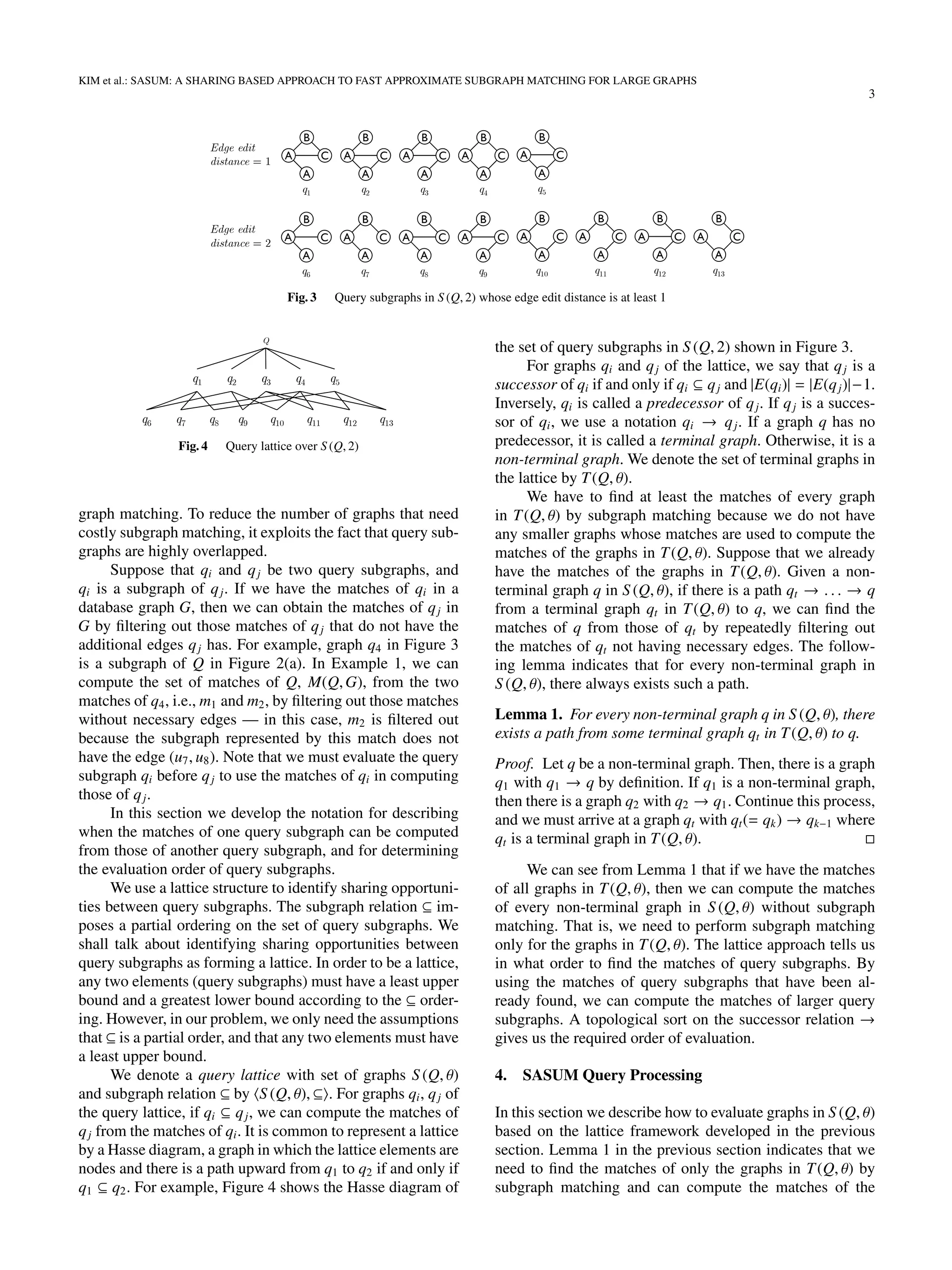
in Figure 2(a) and threshold θ = 2, Figure 3 shows the query
subgraphs in S (Q, 2) whose edge edit distance is at least 1.
Note that Q is also in S (Q, 2).
Definition 5. Given a database graph G and a connected
query graph Q, a connected subgraph g of G is defined as
a match of Q in G if and only if g is graph isomorphic to
Q. Given a positive integer θ as threshold, a connected sub-
graph g of G is defined as an approximate match of Q in G
if and only if g is a match to some query subgraph in S (Q, θ).
We say that a connected subgraph g of G is approximately
isomorphic to Q if g is an approximate match of Q.
For example, in our running example, the subgraph of
G that consists of vertices u1, u2, u3, and u4 is a match of Q.
The one with vertices u4, u7, u8, and u9 is an approximate
match of Q because it is graph isomorphic to graph q4 in
Figure 3.
Given a graph qi, the set of matches in a graph G is
denoted by M(qi,G). A match m in M(qi,G) is represented
as a set of mappings, each of which associates the vertices
of graph qi with the vertices of graph G. A mapping is ex-
pressed as a pair (v, u) where v is in qi and u is in G.
Example 1. Consider the query graph Q and the
database graph G in Figure 2. There is only one
match of Q in G, which is represented as M(Q,G) =
{(v1, u2), (v2, u1), (v3, u4), (v4, u3)}. For graph q4 in Figure
3, there are two matches, i.e., M(q4,G) = {m1, m2}
where m1 = {(v1, u2), (v2, u1), (v3, u4), (v4, u3)} and m2 =
{(v1, u4), (v2, u8), (v3, u7), (v4, u9)}.
We assume that the average degree of the query graph
is at least 2 (i.e., it has at least one cycle in it), since if not,
there is no edge to delete. We also assume θ > 0 to allow
missing edges in approximate matches.
Problem Statement: Given a database graph G, a
query graph Q, and a positive integer threshold θ, our goal is
to efficiently find all graphs that are approximately isomor-
phic to Q in G. In other words, we want to find all matches
of graphs in S (Q, θ) from G.
3. The Lattice Framework
SASUM is a sharing based approach to approximate sub-

3. KIM et al.: SASUM: A SHARING BASED APPROACH TO FAST APPROXIMATE SUBGRAPH MATCHING FOR LARGE GRAPHS
3
3 KAIST Database Lab. ©shkim
Query Subgraphs
q1
A
A
B
C
q2
A
A
B
C
q3
A
A
B
C
q4
A
A
B
C
q5
A
A
B
C
q6
A
A
B
C
q7
A
A
B
C
q8
A
A
B
C
q9
A
A
B
C
q10
A
A
B
C
q11
A
A
B
C
q12
A
A
B
C
q13
A
A
B
C
Edge edit
distance = 1
Edge edit
distance = 2
Fig. 3 Query subgraphs in S (Q, 2) whose edge edit distance is at least 1
4 KAIST Database Lab. ©shkim
Query Lattice
Q
q1 q3 q4 q5
q6 q7 q8 q9 q10
q2
q11 q12 q13
theta = 2
Fig. 4 Query lattice over S (Q, 2)
graph matching. To reduce the number of graphs that need
costly subgraph matching, it exploits the fact that query sub-
graphs are highly overlapped.
Suppose that qi and qj be two query subgraphs, and
qi is a subgraph of qj. If we have the matches of qi in a
database graph G, then we can obtain the matches of qj in
G by filtering out those matches of qj that do not have the
additional edges qj has. For example, graph q4 in Figure 3
is a subgraph of Q in Figure 2(a). In Example 1, we can
compute the set of matches of Q, M(Q,G), from the two
matches of q4, i.e., m1 and m2, by filtering out those matches
without necessary edges — in this case, m2 is filtered out
because the subgraph represented by this match does not
have the edge (u7, u8). Note that we must evaluate the query
subgraph qi before qj to use the matches of qi in computing
those of qj.
In this section we develop the notation for describing
when the matches of one query subgraph can be computed
from those of another query subgraph, and for determining
the evaluation order of query subgraphs.
We use a lattice structure to identify sharing opportuni-
ties between query subgraphs. The subgraph relation ⊆ im-
poses a partial ordering on the set of query subgraphs. We
shall talk about identifying sharing opportunities between
query subgraphs as forming a lattice. In order to be a lattice,
any two elements (query subgraphs) must have a least upper
bound and a greatest lower bound according to the ⊆ order-
ing. However, in our problem, we only need the assumptions
that ⊆ is a partial order, and that any two elements must have
a least upper bound.
We denote a query lattice with set of graphs S (Q, θ)
and subgraph relation ⊆ by S (Q, θ), ⊆ . For graphs qi, qj of
the query lattice, if qi ⊆ qj, we can compute the matches of
qj from the matches of qi. It is common to represent a lattice
by a Hasse diagram, a graph in which the lattice elements are
nodes and there is a path upward from q1 to q2 if and only if
q1 ⊆ q2. For example, Figure 4 shows the Hasse diagram of
the set of query subgraphs in S (Q, 2) shown in Figure 3.
For graphs qi and qj of the lattice, we say that qj is a
successor of qi if and only if qi ⊆ qj and |E(qi)| = |E(qj)|−1.
Inversely, qi is called a predecessor of qj. If qj is a succes-
sor of qi, we use a notation qi → qj. If a graph q has no
predecessor, it is called a terminal graph. Otherwise, it is a
non-terminal graph. We denote the set of terminal graphs in
the lattice by T(Q, θ).
We have to find at least the matches of every graph
in T(Q, θ) by subgraph matching because we do not have
any smaller graphs whose matches are used to compute the
matches of the graphs in T(Q, θ). Suppose that we already
have the matches of the graphs in T(Q, θ). Given a non-
terminal graph q in S (Q, θ), if there is a path qt → . . . → q
from a terminal graph qt in T(Q, θ) to q, we can find the
matches of q from those of qt by repeatedly filtering out
the matches of qt not having necessary edges. The follow-
ing lemma indicates that for every non-terminal graph in
S (Q, θ), there always exists such a path.
Lemma 1. For every non-terminal graph q in S (Q, θ), there
exists a path from some terminal graph qt in T(Q, θ) to q.
Proof. Let q be a non-terminal graph. Then, there is a graph
q1 with q1 → q by definition. If q1 is a non-terminal graph,
then there is a graph q2 with q2 → q1. Continue this process,
and we must arrive at a graph qt with qt(= qk) → qk−1 where
qt is a terminal graph in T(Q, θ).
We can see from Lemma 1 that if we have the matches
of all graphs in T(Q, θ), then we can compute the matches
of every non-terminal graph in S (Q, θ) without subgraph
matching. That is, we need to perform subgraph matching
only for the graphs in T(Q, θ). The lattice approach tells us
in what order to find the matches of query subgraphs. By
using the matches of query subgraphs that have been al-
ready found, we can compute the matches of larger query
subgraphs. A topological sort on the successor relation →
gives us the required order of evaluation.
4. SASUM Query Processing
In this section we describe how to evaluate graphs in S (Q, θ)
based on the lattice framework developed in the previous
section. Lemma 1 in the previous section indicates that we
need to find the matches of only the graphs in T(Q, θ) by
subgraph matching and can compute the matches of the

4. 4
IEICE TRANS. INF. & SYST., VOL.Exx–??, NO.xx XXXX 200x
5
T(Q,θ)
B(Q,θ) q1 q2
S(Q,θ)
Bseed(Q,θ)={q1,q2}
Q
Edge edit
distance = 0
Base graph generation
and seed selection
Query evaluation...
Edge edit
distance = 1
Fig. 5 Overview of SASUM query processing
other graphs in S (Q, θ) from them. Although the number of
graphs in T(Q, θ) is smaller than that of graphs in S (Q, θ),
it can still be large. For example, if a query graph Q has m
edges, the number of graphs in T(Q, θ) could be O(mθ
).
To further reduce the number of graphs that need exact
subgraph matching, SASUM generates a set of graphs called
base graphs, denoted by B(Q, θ), that are shared by terminal
graphs in T(Q, θ) by further deleting edges. Then it chooses
the minimum number of base graphs whose matches are
used to compute the matches of all graphs in T(Q, θ). The
selected base graphs are called seed graphs, and the set of
seed graphs are denoted by Bseed(Q, θ). The number of seed
graphs in Bseed(Q, θ) is less than or at most equal to the num-
ber of terminal graphs in T(Q, θ) (we will provide a proof in
Section 5), and it is much smaller in many cases. SASUM
first finds the matches of the seed graphs by subgraph match-
ing and then systematically computes the matches of all
graphs in S (Q, θ). This sharing based approach of SASUM
leads to much reduction in the number of graphs that need
costly exact subgraph matching.
Query processing in SASUM consists of three phases:
base graph generation, seed selection, and query evalua-
tion. Figure 5 shows an overview of query processing in
SASUM. In the base graph generation phase, SASUM gen-
erates the set of base graphs B(Q, θ) from the terminal
graphs in T(Q, θ). In the seed selection phase, it chooses
the seed graphs from the base graphs. Finally, in the query
evaluation phase, SASUM finds the matches of every graph
in S (Q, θ) from the matches of the seed graphs. We describe
each phase in more detail in the subsequent sections.
4.1 Base Graph Generation
SASUM generates a set of base graphs that are shared by ter-
minal graphs through the operation of deleting edges called
edge pruning, which is defined as follows:
Definition 6. In a graph G, pruning of edge e is the deletion
of edge e and, if any, an isolated vertex (i.e., a vertex of
degree 0) such that the resulting graph G − e is connected
and has one less edge than G.
For example, Figure 6 shows the results of pruning of
edges e1 and e3 from G. Note that in G − e2, the isolated
vertex labeled ‘A’ has been removed. G − e1 has one less
edge than G, whereas G − e3 has one less edge than G and
also one less vertex.
G – e1
A
A
B
C
G – e3
A
A
B
C
e3
G
A
A
B
C
e1
Fig. 6 An example of edge pruning
8 KAIST Database Lab. ©shkim
폰트 기준:
- 라벨: Gill Sans MT, 14pt
- 내용: Euclid, 16pt
- caption: Euclid, 14pt
(윤곽)선 두께: 1pt
q
q1 q3 q4 q5
q6 q7 q8 q9 q10
q2
q11 q12 q13
q14 q15 q16 q17 q18 q19 q20 q21
theta = 2
seed: 14 15 16 21
T(Q,2)
B(Q,2)
Fig. 8 How the base graphs in B(Q, 2) cover the terminal graphs in
T(Q, 2)
Lemma 2. Given a connected graph G with at least one
edge, edge pruning, G − e, always produces at least one
graph with one less edge than G.
Proof. Assume that a graph G has a cycle in it. Then, we
can delete any edge e in the cycle and obtain a graph G − e
with one less edge than G. Now assume that G has no cycle
in it. Then it must be a tree (connected, acyclic graph). A
leaf in a tree is a vertex of degree 1. Every tree with at least
one edge has at least two leaves [11]. Take any leaf v, and
delete the edge e attached to it and the vertex v itself. Then
we obtain a new graph G −e with one less edge and one less
vertex.
Let B(Q, θ) denote the set of base graphs obtained by
pruning of a single edge from the graphs in T(Q, θ). Figure
7 shows the base graphs generated by edge pruning from the
graphs in T(Q, 2). For example, graph q14 can be obtained
by either pruning of edge e3 from graph q6, or edge e5 from
graph q9. Note that a base graph in B(Q, θ) may be shared
by one or more terminal graphs in T(Q, θ) as you can see in
this example.
4.2 Seed Selection
We formally state the seed selection problem where we want
to select the minimum number of base graphs in B(Q, θ)
whose matches are used to compute the matches of every

5. KIM et al.: SASUM: A SHARING BASED APPROACH TO FAST APPROXIMATE SUBGRAPH MATCHING FOR LARGE GRAPHS
5
7
q14
A
B
C
q15
A
A
B
q16
A
A
C
q17
A
B
C
q18
A
B
C
q19
A
A
C
q20
A
A
C
q21
A
B
C
Fig. 7 Base graphs generated from the graphs in T(Q, 2)
graph in T(Q, θ). We say that a base graph qb covers a ter-
minal graph qt if qb ⊆ qt. We denote the set of terminal
graphs in T(Q, θ) that are covered by a base graph qb in
B(Q, θ) by C(qb). Now we are required to find the small-
est subset Bseed(Q, θ) of B(Q, θ) such that the seed graphs in
Bseed(Q, θ) collectively cover every graph in T(Q, θ): that is,
T(Q, θ) = q∈Bseed(Q,θ) C(q).
It is easy to see that the seed selection problem reduces
to the set cover problem [2], whose decision version is NP-
Complete. An instance of the set cover problem consists of
a finite set U and a collection S of subsets of U, such that
every element of U belongs to at least one subset in S . We
want to find the smallest subset C of S whose union is U.
The seed selection problem is transformed into the set cover
problem by setting U = T(Q, θ) and S = {C(q)|q ∈ B(Q, θ)}.
The set cover problem requires that every element of U be-
longs to at least one subset in S , which is guaranteed by
Lemma 2.
There is a greedy approximation algorithm for the set
cover problem whose approximation ratio is ln |U| + 1 [12].
This algorithm begins by selecting the largest subset from S
and then deletes all its elements from U. The algorithm adds
the subset containing the largest number of remaining un-
covered elements repeatedly until all elements are covered.
In the seed selection phase, SASUM obtains Bseed(Q, θ)
from B(Q, θ) by using the greedy approximation algorithm
just described.
Example 2. Figure 8 shows how the base graphs in B(Q, 2)
cover the terminal graphs in T(Q, 2). There is an edge be-
tween a base graph and a terminal graph if the base graph
covers the terminal graph. If we apply the greedy approx-
imation algorithm to the base graphs in B(Q, 2), the algo-
rithm selects the base graphs in the following order: q15,
q21, q14, and q16. Thus we have Bseed(Q, 2) = {q14, q15, q16,
q21}, the size of which is only half of the size of T(Q, 2).
4.3 Query Evaluation
In this section we describe how to find the matches of all
graphs in S (Q, θ). SASUM first finds the matches of graphs
in Bseed(Q, θ) by exact subgraph matching. Any exact sub-
graph matching algorithm can be used for this purpose. Then
from these matches, it computes the matches of all graphs
in T(Q, θ). Given a graph qt in T(Q, θ), the matches of any
graph qb in Bseed(Q, θ) can be used to compute the matches
of qt if qt is in C(qb). According to Lemma 1, the matches of
graphs in T(Q, θ) can be used to compute the matches of the
other graphs in S (Q, θ). To reuse matching results, we have
to determine the evaluation order of graphs in S (Q, θ) such
that if qi → qj, we find the matches of qi first. By topolog-
ically sorting the query lattice S (Q, θ), ⊆ on the successor
relation →, we can obtain the required evaluation order of
graphs.
Let the determined order be q1 → q2 → · · · → qk
where k = |S (Q, θ)|. SASUM finds the matches of graphs in
this order. If a graph q is a terminal graph in T(Q, θ), then
SASUM already has computed the matches of q against the
database graph G. If a query subgraph q is a non-terminal
graph in S (Q, θ), SASUM finds the matches of q from the
matches of q’s predecessors in the query lattice. It is guar-
anteed that the matches of these predecessors have already
been found by the topological sorting order of graphs over
the successor relation →. We can reuse the matches of any
predecessor graph here. To speed up the process of com-
puting matches by reducing the size of intermediate match-
ing results, SASUM uses the predecessor graph q∗
with the
smallest number of matches, i.e., q∗
= arg minq {|M(q ,G)| :
q → q} to compute the matches of q.
Example 3. In Figure 4, the matches of q4 can be com-
puted from the matches of any one of graphs q7, q10, q11,
and q13. The number of matches of these graphs are as fol-
lows: |M(q7,G)| = 5, |M(q10,G)| = 4, |M(q11,G)| = 2, and
|M(q13,G)| = 6. Therefore, SASUM computes the matches
of q4 from those of q11.
Now we describe how to compute the matches of a
graph from those of another graph. There are two cases
to consider when reusing matching results: (1) from the
matches of a graph in Bseed(Q, θ) to those of a graph in
T(Q, θ), and (2) from the matches of a graph in S (Q, θ)
to another graph in S (Q, θ). We consider the case (2) first.
When qi and qj are both in S (Q, θ) and qi → qj, then graph
qj has one additional edge than graph qi. In this case, for
each match in M(qi,G), SASUM checks whether that match
has the additional edge and prunes those matches not having
that edge.
We now discuss the case (1). When qi is in Bseed(Q, θ),
qj is in T(Q, θ), and qj is in C(qi), then qj has either (i) one
additional edge, or (ii) one additional edge and one addi-
tional vertex since qi is generated by edge pruning. For the
case (i), SASUM does the same as in the case (2) above. For
the case (ii), however, we cannot compute the matches of qj
by only pruning the matches of qi. Instead, we have to ex-
tend the matches of qi with the mappings of the additional
vertex. Let graph qj have n vertices and qi have n−1 vertices.
Given a match m in M(qi,G), let vertices u1, u2, . . . , un−1 in
G are the mappings of vertices v1, v2, . . . , vn−1 in qi. Suppose
that vn is an additional vertex in qj, and there is an additional
edge (vi, vn) in qj where 1 ≤ i ≤ n − 1. Now we extend the

6. 6
IEICE TRANS. INF. & SYST., VOL.Exx–??, NO.xx XXXX 200x
match m with the mappings (vn, un) for un in G such that the
edge (ui, un) exists in E(G), and the label of un is equal to
that of vn, i.e., l(un) = l(vn). We can easily find such un’s
from G by visiting the adjacent vertices uj of ui and check-
ing whether l(uj) = l(vn).
Example 4. We illustrate how to compute matches from
other matches by an example, shown in Figure 9. In this
example, we shall compute the matches of graphs q6 and
q1 from those of seed graph q14. On the left, we show the
query graph Q and the database graph G again for the con-
venience of the reader. On the right, we show the graphs
q14, q6, and q1 where q14 covers q6, and q6 → q1. The set
of matches of a graph is shown below the graph, as a ta-
ble. The first row of a table shows the vertices in the graph
above it, and the remaining rows represent the matches of
the graph. We use m1, m2, . . . to denote the first match (row),
the second match, and so on, in each set of matches.
Assume that we already have found the matches
in M(q14,G) by subgraph matching. Now we compute
M(q6,G) from M(q14,G). In the figure, graph q6 has one
additional edge (v1, v3) and one additional vertex v3 than
graph q14 (indicated by using solid lines). Thus, we need to
compute M(q6,G) from M(q14,G) by extending each match
in M(q14,G) with the mappings of vertex v3. Let us consider
the match m1 = {(v1, u2), (v2, u1), (v4, u3)} first. Since the ad-
ditional edge is between vertices v1 and v3, and the label
of vertex v3 is ‘A’, we find the adjacent vertices of u2 in G
having label ‘A’. Only vertex u4 is eligible as the mapping of
vertex v3. Thus, the match m1 in M(q14,G) is extended by the
mapping (v3, u4) to be the match m1 in M(q6,G). The other
matches in M(q14,G) can be extended in the same way just
described. A dotted arrow from a match m in M(q14,G) to a
match m in M(q6,G) indicates that the match m is extended
to be the match m .
Next we compute M(q1,G) from M(q6,G). The graph
q1 has one additional edge (v2, v4) than q6. Here we com-
pute M(q1,G) by filtering out those matches in M(q6,G)
not having the edge corresponding to the edge (v2, v4) in G.
The matches m2 and m3 in M(q6,G) are filtered out because
there is no edge between vertices u8 and u3.
4.4 Outputting Matching Results
In the problem statement present in Section 2, we do not im-
pose any restrictions on the order of outputting the matching
results of the graphs in S (Q, θ). However, the user may want
to get the matching results in the order of the edge edit dis-
tance from the query graph: that is, the matching results of
the query graph, and those with one missing edge, those with
two missing edges, and so on. In this case, we must keep the
matching results of every graph in S (Q, θ) before outputting
them.
If the user does not care about the order of outputting
results, then SASUM can reduce the space usage by pro-
ducing and removing intermediate matching results early.
There are two cases to consider. First, let q be a graph
in Bseed(Q, θ). If SASUM has obtained the matches of all
graphs q where q is in C(q), then SASUM can safely throw
away the matches of q because they will not be used later.
Second, let q be a graph in S (Q, θ). If SASUM has ob-
tained the matches of all graphs that are successors of q,
then SASUM can remove the matches of q right away for
the same reason.
5. Analytical Study
This section analyzes our approach to approximate subgraph
matching. We aim at proving the correctness of SASUM and
showing the superiority of our approach compared to the
state-of-the-art method in terms of the number of graphs that
need subgraph matching.
5.1 Proof of correctness
The following theorem shows the correctness of SASUM.
Theorem 1. Given a database graph G, a connected query
graph Q, and a positive integer threshold θ, SASUM finds
all matches of graphs in S (Q, θ).
Proof. In the evaluation phase, SASUM first finds the
matches of graphs in Bseed(Q, θ) by subgraph matching.
Then it computes the matches of graphs in T(Q, θ) from
those of graphs in Bseed(Q, θ). Now it remains to show
whether SASUM correctly computes the matches of all non-
terminal graphs in S (Q, θ). According to Lemma 1, for ev-
ery non-terminal graph q in S (Q, θ), there is a path from
some terminal graph qt in T(Q, θ) to q. Let the path be
q1(= qt) → q2 → · · · → qk(= q). By the evaluation or-
der of graphs, which is a topological order, the matches of
qi is computed from those of qi−1 for 2 ≤ i ≤ k. We already
have the matches of qt. Therefore, SASUM computes the
matches of q eventually.
5.2 Performance Guarantee of SASUM
We compare SASUM with the state-of-the-art approach in
terms of the number of graphs that need costly subgraph
matching. The number of graphs that need subgraph match-
ing is a dominant factor in the overall performance of a given
method for approximate subgraph matching (we will ver-
ify this in Section 6 through experimental evaluation). We
compare three approaches: NAIVE, SHARE, and SASUM.
The NAIVE approach is the one that finds the matches of
each graph in S (Q, θ) independently. The SHARE approach
is a basic sharing based approach, which is employed by
the state-of-the-art method [10]. It computes the matches
of a query subgraph from those of another query subgraph.
SHARE needs subgraph matching for the graphs in T(Q, θ).
Our approach, SASAUM, increases sharing opportunities by
generating base graphs and selecting a small number of seed
graphs. SASUM needs subgraph matching for the graphs
in Bseed(Q, θ). Let CNAIVE, CSHARE, and CSASUM denote the

7. KIM et al.: SASUM: A SHARING BASED APPROACH TO FAST APPROXIMATE SUBGRAPH MATCHING FOR LARGE GRAPHS
7
8 KAIST Database Lab. ©shkim
u2 u1 u3
v1 v2 v4
M(q14,G)
u4 u8 u3
u4 u8 u5
u2 u1 u4
v1 v2 v3
M(q6,G)
u4 u8 u2
u4 u8 u7
u3
v4
u3
u5
u4 u8 u7
u4 u8 u2
u3
u5
u2 u1 u4
v1 v2 v3
M(q1,G)
u4 u8 u7
u3
v4
u5
u4 u8 u2 u5
q1q6q14
Extend Filter out
A
B
C A
A
B
CA
e1
e2
e3
e4
v1
v2
v4
v3
A
B
C
e5
A
A
B
C
e3
v3
v1
v2
e4
u1
u2 u3
u4
u5 u6
u7 u8
u9
A
A
B
C
A
C
B
C D
G
Q
v4
Fig. 9 Computing the matches of graphs q6 and q1 from those of graph q14
number of graphs that need subgraph matching by NAIVE,
SHARE, and SASUM, respectively.
It is easy to see that CSHARE < CNAIVE because
T(Q, θ) ⊂ S (Q, θ). The following theorem shows that
SASUM needs no more graphs than SHARE that need sub-
graph matching:
Theorem 2. CSASUM ≤ CSHARE.
Proof. We shall show |Bseed(Q, θ)| ≤ |T(Q, θ)|. SASUM se-
lects the seed graphs in Bseed(Q, θ) from the base graphs in
B(Q, θ) by transforming the seed selection problem into the
set cover problem and using the greedy approximation algo-
rithm for the set cover problem, as described in Section 4.2.
The greedy approximation algorithm selects one graph from
B(Q, θ) at a time, and removes the graphs covered by the
selected graph from T(Q, θ). Since every graph in B(Q, θ)
covers at least one graph in T(Q, θ) (by Lemma 2), at least
one graph is removed from T(Q, θ) at each iteration of the
greedy approximation algorithm. Hence, the number of seed
graphs in Bseed(Q, θ) selected by the greedy approximation
algorithm is bounded by the number of terminal graphs in
T(Q, θ), that is, |Bseed(Q, θ)| ≤ |T(Q, θ)|.
6. Experimental Evaluation
6.1 Setup
We implemented our algorithm as a single threaded exe-
cutable in C++. We compare our method with SAPPER
[10], the state-of-the-art method for approximate subgraph
matching. SAPPER evaluates the graphs in S (Q, θ) in the
depth first search order and finds the matches of a graph q
in S (Q, θ) from the matches of another graph q in S (Q, θ)
where q → q, similar to our approach. However, SAP-
PER always performs subgraph matching for every graph
in T(Q, θ), and which q to use is predetermined. We down-
loaded an executable of SAPPER from the authors’ web-
site†
. We used the same exact subgraph matching algorithm
†
http://sites.google.com/site/shijiezhang/Home/grapham-a-graph-
approximate-matching-tool (accessed on April 12, 2011)
Table 1 Default Parameter Values
Parameter Default value
Number of vertices |V(G)| in G 5000
Average degree deg(G) of G 8
Number of distinct labels |L(G)| 250
Number of vertices |V(Q)| in Q 20
Average degree deg(Q) of Q 3
θ 1
used in SAPPER when implementing SASUM. All exper-
iments were performed on a machine with Intel Xeon(R)
CPU E5345 2.33GHz and 8GB main memory, running
on Fedora 12 Linux operating system. We used synthetic
datasets and two real-world datasets in the experiments.
6.2 Synthetic Datasets
We first compare the two approaches on synthetic datasets.
We generated synthetic datasets with a graph generator,
gengraph [13]††
. The default values of the parameters are
listed in Table 1. Synthetic graphs generated by the graph
generator have a heavy tailed degree sequence (i.e., a se-
quence of vertex degrees in descending order) to model real
datasets†††
.
We analyze the performance of SASUM and SAPPER
by independently varying each of |V(G)|, |L(G)|, θ, |V(Q)|,
and deg(Q). The results are shown in Figure 10 and 12. In
Figure 10, SASUM outperforms SAPPER in all cases. In
particular, consider the case when the database graph is large
(in Figure 10(a)) and the number of distinct labels is small
(in Figure 10(b)) where subgraph matching requires much
time. In this case, SASUM performs far better than SAP-
PER because SASUM requires a less number of graphs that
need subgraph matching. In Figure 10(c) and Figure 10(d),
we vary threshold θ in two different sets of database graphs.
As we can see in the figures, SASUM outperforms SAP-
PER by orders of magnitude because SASUM requires a far
††
downloaded at http://fabien.viger.free.fr/liafa/generation/
†††
We also used graphs whose degree distribution of vertices is
uniform. We obtained similar results, thus do not include the results
here.

8. 8
IEICE TRANS. INF. & SYST., VOL.Exx–??, NO.xx XXXX 200x
0
1
2
3
4
5
2500 5000 7500 10000
Runtime(sec)
Number of vertices in G
SASUM
SAPPER
(a) Varying |V(G)|
0
2
4
6
8
10
12
14
16
18
20
0 100 200 300
Runtime(sec)
Number of labels in G
SASUM
SAPPER
(b) Varying |L(G)|
0.1
1
10
100
1000
10000
1 2 3
Runtime(sec)
θ
SASUM
SAPPER
(c) Varying θ (|V(G)| = 5000, |V(Q)| =
20) (Log scale)
0.01
0.1
1
10
100
1000
1 2 3
Runtime(sec)
θ
SASUM
SAPPER
(d) Varying θ (|V(G)| = 2500, |V(Q)| =
10) (Log scale)
Fig. 10 Query execution time for synthetic datasets
0
0.1
0.2
0.3
0.4
0.5
0.6
0.7
0.8
0.9
1
1 2 3
Reductionratio
θ
|V(Q)| = 20
Fig. 11 Comparing the number of subgraph matching executions
0
0.5
1
1.5
2
2.5
3
3.5
4
10 20 30
Runtime(sec)
Number of vertices in Q
SASUM
SAPPER
(a) Varying |V(Q)|
0
0.5
1
1.5
2
2.5
3
3.5
4
4.5
5
5.5
2 3 4
Runtime(sec)
Degree of Q
SASUM
SAPPER
(b) Varying deg(Q)
Fig. 12 Query execution time for different query graphs
less number of graphs that need subgraph matching. When
threshold θ is large, the number of graphs in T(Q, θ) is large,
but SASUM uses Bseed(Q, θ) instead, which is far smaller
than T(Q, θ). We can verify this in Figure 11, which shows
the reduction ratio of SASUM in the number of graphs that
need subgraph matching. For example, the reduction ratio of
0.6 indicates that SASUM reduces the number of graphs that
need subgraph matching by 60% when compared to SAP-
PER. As you can see in the figure, SASUM requires less
than half the number of graphs that need subgraph match-
ing required by SAPPER in all cases, and as θ increases, the
reduction ratio further increases.
We vary the number of vertices in Q and, the results are
shown in Figure 12(a). With more vertices in Q, more ver-
tices and edges need to be compared in subgraph matching.
Thus the query times of both methods increase. However,
SASUM performs better than SAPPER because it requires
a smaller number of graphs that need subgraph matching.
0
20
40
60
80
100
2500 5000 7500 10000
Relativeportion(%)
Number of vertices in G
Exact subgraph matching
The other parts
(a) Varing |V(G)|
0
20
40
60
80
100
1 2 3
Relativeportion(%)
θ
Exact subgraph matching
The other parts
(b) Varing θ
Fig. 13 Breakdown of query execution time
The last parameter we vary is the average degree of Q.
The results are shown in Figure 12(b). A high vertex degree
generates more graphs in S (Q, θ) since the number of graphs
in S (Q, θ) is exponential to the average degree of Q. And
when the average degree of Q is large, subgraph matching
needs to compare more edges. Thus, as the average degree
of Q increases, the performance gap between SASUM and
SAPPER widens.
We analyze query execution time of SASUM to ac-
cess relative portion of time spent at subgraph matching and
that spent at the other parts. The results are shown in Fig-
ure 13(a) and (b). Figure 13(a) shows the portion of time
spent by subgraph matching and the other parts in the over-
all query execution time. As the number of vertices in G
increases, subgraph matching needs to compare more ver-
tices. Thus, the portion of time spent by subgraph matching
increases and dominates the overall performance. In Figure
13(b), we vary threshold θ. Here the portion of time spent by
the other parts increases as θ increases. This is because the
number of graphs in S (Q, θ) is exponential to θ. Neverthe-
less, the portion of time spent by subgraph matching is still
dominant in all cases.
6.3 Real datasets
For real world data, we prepared two large real graphs: a
human protein interaction network [14] and a collabora-
tion network [15]. The protein interaction network contains
10,527 vertices and 40,903 edges. Each vertex represents a
protein, and the label of the vertex is its gene ontology term.
An edge in the graph represents an interaction between the
two proteins it connects. The collaboration network includes
5,241 vertices and 14,484 vertices. Each vertex represents
an author, and there is an edge between two authors if they
coauthored a paper. 250 labels are randomly distributed over
the vertices in the collaboration network. Figure 14 shows

9. KIM et al.: SASUM: A SHARING BASED APPROACH TO FAST APPROXIMATE SUBGRAPH MATCHING FOR LARGE GRAPHS
9
0
100
200
300
400
500
600
700
Degree
Vertices in descending order of degree
(a) Human protein interaction
network
0
10
20
30
40
50
60
70
80
90
Degree
Vertices in descending order of degree
(b) Collaboration network
Fig. 14 Degree sequences of real graphs
1
10
100
1000
10000
100000
1 2 3
Runtime(sec)
θ
SASUM
SAPPER
(a) Human protein interaction
network (Log scale)
0.1
1
10
100
1000
10000
1 2 3
Runtime(sec)
θ
SASUM
SAPPER
(b) Collaboration network (Log
scale)
Fig. 15 Query execution time with real graphs
sample degree sequences of the two real datasets. As you
can see in the figure, their degree sequences show a heavy-
tail behavior.
We compare the performance of SASUM and SAPPER
over different query graphs extracted from the two graphs.
Since most of the results are similar to those for the syn-
thetic datasets, we show the results of varying only thresh-
old θ, which are shown in Figure 15. The figure shows that
SASUM outperforms SAPPER by orders of magnitude in
terms of query execution time in both datasets.
7. Related Work
Subgraph matching, which finds the occurrences of a spec-
ified graph pattern in a graph, is a fundamental operation
in graph data processing. Ullmann [3] proposed a subgraph
matching algorithm based on a state space search method
with backtracking. VF2 [4] is a more recent work that intro-
duces a set of feasibility rules for pruning the state space.
These two methods, however, are prohibitively expensive
for query processing against a large database graph since
they do not use any index structure by preprocessing the
database graph.
Several indexing based method have been developed
for subgraph matching. In graph indexing methods, e.g.,
GraphGrep [16], gIndex [17], TreePi [18], Tree+∆ [19], and
FG-Index [20], the graph database consists of a set of small
graphs. The goal of graph indexing is to find all graphs that
contain a given query graph. On the other hand, subgraph in-
dexing finds all occurrences of a given query graph in a very
large database graph. GADDI [5], NOVA [6], SUMMA [7],
the approach proposed in [8], and SAPPER [10] fall into
this category. Our approach, SASUM, also belongs to this
category.
Recently, a number of methods have been proposed to
support approximate subgraph matching [10,21,22]. Among
them, similarity search methods, e.g., TALE [21] and G-
Hash [22], are not designed to find all approximate matches
of a given query graph. SAPPER [10] is the state-of-the-art
method that finds all approximate matches of a given query
graph from a large database graph. SAPPER uses the fact
that subgraphs of a given query are highly overlapped. It
finds the matches of a larger graph from those of a smaller
graph. However, SAPPER still needs to perform subgraph
matching for a large number of graphs.
8. Conclusions
In this paper we have investigated how to find all approxi-
mate matches of a given graph from a large database graph,
allowing missing edges. A straightforward way to solve this
problem is to generate a set of query subgraphs, which have
no more missing edges than a user-specified threshold, and
perform subgraph matching for each query subgraph inde-
pendently. However, this simple method is not feasible be-
cause the number of query subgraphs could still be too large,
and subgraph matching itself is a very difficult problem.
In this paper we have proposed a sharing based
approach to fast approximate subgraph matching, called
SASUM. We aim at reducing the number of graphs that
need subgraph matching, which decides the overall perfor-
mance of an approximate subgraph matching algorithm. To
this end, SASUM exploits the fact that query subgraphs are
highly overlapped. Due to this property of query subgraphs,
the matches of a query subgraph can be computed from
those of another query subgraph without costly subgraph
matching. SASUM uses a lattice framework to identify shar-
ing opportunities between query subgraphs. SASUM goes
one step further and produces small base graphs that are
shared by query subgraphs by edge pruning. It then chooses
a small number of seed graphs from them, and performs sub-
graph matching only for the seed graphs. SASUM system-
atically computes the matches of all query subgraphs from
those of seed graphs. We have proven that the number of
graphs that need subgraph matching required by SASUM
is less than or at most equal to the number required by the
state-of-the-art method; and it is much smaller in many cases
as shown through the experimental evaluation. A compre-
hensive set of experiments has shown that SASUM outper-
forms the state-of-the-art method by orders of magnitude in
terms of query execution time due to great reduction in the
number of graphs that need subgraph matching.
References
[1] T. Keshava Prasad, R. Goel, K. Kandasamy, S. Keerthikumar, S. Ku-
mar, S. Mathivanan, D. Telikicherla, R. Raju, B. Shafreen, A. Venu-
gopal, et al., “Human protein reference database—2009 update,”
Nucleic Acids Res., vol.37, no.suppl 1, pp.D767–D772, 2009.
[2] M. Garey and D. Johnson, Computers and Intractability: A Guide
to the Theory of NP-completeness, WH Freeman & Co. NY, USA,
1979.
[3] J. Ullmann, “An algorithm for subgraph isomorphism,” J. ACM,

10. 10
IEICE TRANS. INF. & SYST., VOL.Exx–??, NO.xx XXXX 200x
vol.23, no.1, pp.31–42, 1976.
[4] L. Cordella, P. Foggia, C. Sansone, and M. Vento, “A (sub) graph
isomorphism algorithm for matching large graphs,” IEEE Trans. Pat-
tern Anal. Mach. Intell., vol.26, no.10, pp.1367–1372, 2004.
[5] S. Zhang, S. Li, and J. Yang, “Gaddi: distance index based subgraph
matching in biological networks,” Proc. EDBT, pp.192–203, 2009.
[6] K. Zhu, Y. Zhang, X. Lin, G. Zhu, and W. Wang, “Nova: A novel and
efficient framework for finding subgraph isomorphism mappings in
large graphs,” Proc. DASFAA, pp.140–154, 2010.
[7] S. Zhang, S. Li, and J. Yang, “Summa: subgraph matching in mas-
sive graphs,” Proc. CIKM, pp.1285–1288, 2010.
[8] S. Kim, I. Song, and Y. Lee, “An edge-based framework for fast
subgraph matching in a large graph,” Proc. DASFAA, pp.404–417,
2011.
[9] S. Suthram, T. Shlomi, E. Ruppin, R. Sharan, and T. Ideker, “A direct
comparison of protein interaction confidence assignment schemes,”
BMC Bioinf., vol.7, no.1, p.360, 2006.
[10] S. Zhang, J. Yang, and W. Jin, “Sapper: subgraph indexing and ap-
proximate matching in large graphs,” Proc. VLDB Endow., vol.3,
no.1-2, pp.1185–1194, 2010.
[11] D.B. West, Introduction to Graph Theory, Prentice Hall, 2001.
[12] T. Cormen, Introduction to algorithms, MIT electrical engineering
and computer science series, MIT Press, 2001.
[13] F. Viger and M. Latapy, “Efficient and simple generation of random
simple connected graphs with prescribed degree sequence,” Com-
puting and Combinatorics, pp.440–449, 2005.
[14] C. Stark, B. Breitkreutz, A. Chatr-aryamontri, L. Boucher,
R. Oughtred, M. Livstone, J. Nixon, K. Van Auken, X. Wang, X. Shi,
et al., “The biogrid interaction database: 2011 update,” Nucleic acids
research, vol.39, no.suppl 1, pp.D698–D704, 2011.
[15] J. Leskovec, J. Kleinberg, and C. Faloutsos, “Graph evolution: Den-
sification and shrinking diameters,” ACM Trans. Knowledge Dis-
covery from Data, vol.1, no.1, pp.2:1–2:41, 2007.
[16] D. Shasha, J.T.L. Wang, and R. Giugno, “Algorithmics and applica-
tions of tree and graph searching,” Proc. PODS, pp.39–52, 2002.
[17] X. Yan, P. Yu, and J. Han, “Graph indexing: A frequent structure-
based approach,” Proc. SIGMOD, pp.335–346, 2004.
[18] S. Zhang, M. Hu, and J. Yang, “Treepi: A novel graph indexing
method,” Proc. ICDE, pp.966–975, 2007.
[19] P. Zhao, J. Yu, and P. Yu, “Graph indexing: tree + delta >= graph,”
Proc. VLDB, pp.938–949, 2007.
[20] J. Cheng, Y. Ke, W. Ng, and A. Lu, “Fg-index: towards verification-
free query processing on graph databases,” Proc. SIGMOD, pp.857–
872, 2007.
[21] Y. Tian and J. Patel, “Tale: A tool for approximate large graph
matching,” Proc. ICDE, pp.963–972, 2008.
[22] X. Wang, A. Smalter, J. Huan, and G. Lushington, “G-hash: towards
fast kernel-based similarity search in large graph databases,” Proc.
EDBT, pp.472–480, 2009.