1. 1
Root – Locus Technique
A root- locus analysis is analytical method for displaying graphically in
the s- plane , the location of the poles of the closed – loop T.F as
function of the gain factor K of the open- loop T.F
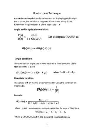
Angle and Magnitude conditions:
Angle condition:
The condition on angles are used to determine the trajectories of the
root loci in the s- plane
Magnitude condition:
The values of K on the loci are determined by using the condition on
magnitude .
Example:
2. 2
Construction of the root loci:
1 - Each locus starts at an open- loop pole when k = 0 and finishes either
at an open – loop zero or ∞ , when k = ∞
2 - The number of branches of the root loci is equal to the order system
3 - Points of the root –locus on the real axis lie to the left of an odd
number of finite poles and zeros for k>0.Loci either move along the real
axis or occur as complex conjugate pairs of loci
4 - The root loci are symmetrical with respect to the real axis of plane
5 – Angle and center of asymptotes:
3. 3
6 - Breakaway points (saddle points)
The breakaway point between two poles or break -in point between two
zeros is a point on the real axis where two or more branches of the root-
locus depart from or arrive at the real axis
Note: A root locus plot may have more than one breakaway point.
Breakaway points may be complex conjugates
7- Departure and arrival angles:
The angle of departure from a complex pole or angle of arrival at the
complex zero (ignoring the contribution of that pole or zero) is given by
Angle of departure = 180 + ( ɸz - Өp )
Angle of arrival = 180 - ( ɸz - Өp )
Example:
Find the angle of departure
4. 4
Solution: 180 + (45 – 90) = 135
8 – Intersection of the root loci with the imaginary axis and calculation of
k and frequency of oscillation ω
The limiting value of k for stability may be found using the routh array
on the characteristic equation
Example: Consider the system shown in figure below . Sketch the root –
locus plot and then determine the value of k such that the damping
ratio of a pair of dominant poles is 0.5
Solution:
The open – loop T.F G(s) H(s) =
Number of open – loop poles n= 3
Number of open – loop zeros m=0
3rd
order system, The number of loci (branches) = n =3
number of asymptotes = n-m = 3-0=3
The number of asymptotes angles = n -m =3-0=3
5. 5
Angle and center of asymptotes:
i = 0 , 1 , 2 : Ө0 = 60 , Ө1 = 180 , Ө2 = 300 = - 60
Center of asymptotes = ( - 1 -2 ) - 0 / (3 - 0) = - 1
Breakaway points : The characteristic equation is:
K = S3
+ 3S2
+ 2S
dK / dS = 3S2
+6S +2 = 0 notes s= -1.5774 neglected
6. 6
The crossing points on the imaginary axis
The characteristic equation is:
The routh array becomes
The value of K at breakaway points s = - 0.4226 is 0.384
0<K<0.384 overdamped , K =0.384 critical damped , 0.384<K<6 underdamped
K = 6 critical stable , K > 6 unstable system
7. 7
Example :Consider the control system shown in figure below. Sketch the
root – locus plot and determine the approximate damping ratio for a
value of K = 1.33
Solution:
n=2 , m = 1 , 2nd
order system , 2 loci , 1 asymptotes , 1 angle ,Ө0=180
The angle of departure is
8. 8
The characteristic equation is:
S2
+ ( 2 + K ) S + 3 + 2K = 0 , for K = 1.33
S2
+ 3.33 S + 5.66 = 0 , S1 = - 1.665 + J 1.699 , ω = 1.699 , α =1.665
ө = tan -1
= ω/ α = 450
, ζ =0.707
Example: Sketch the root – locus plot for the system shown in figure below
Solution:
11. 11
Example: Sketch the root locus for the system shown in fig below.
Solution:
Center of asymptotes
Angles of asymptotes = 60 , 180 , 300
The closed-loop T.F
For stability 90-k>0, 21k>0 -k2
-65k+720 / 90-k >0
From equation
dk/ds=3s4
+26s3
+77s2
+84s+24 breakaway point =-0.43
( 90-9.65)s2
+21(9.65)= 0 ω=1.59 rad/sec