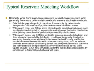
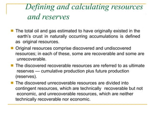
The document discusses the processes of oil and gas formation, detailing the role of kerogen, bitumen, and petroleum generation via temperature and time. It distinguishes between conventional and unconventional oil, highlighting the need for advanced recovery methods due to the depletion of conventional reserves, and outlines the significance of sedimentary basins in hydrocarbon generation. Additionally, it explores the properties of various sedimentary rocks, which serve as reservoir and source rocks for oil and gas, emphasizing the importance of understanding sediment characteristics in petroleum geology.


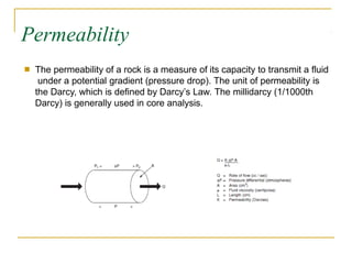
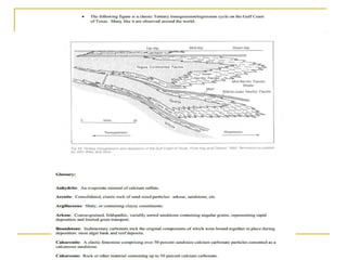
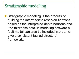
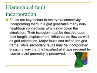
![Sources of unconventional
oil
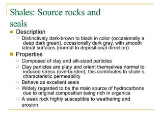
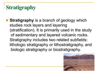
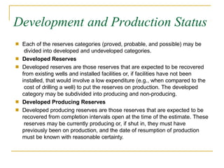
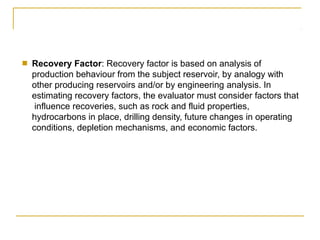
■ According to the International Energy Agency's Oil Market
Report unconventional oil includes the following sources:
Oil shales
Oil sands-based synthetic crudes and derivative products
Coal-based liquid supplies
Biomass-based liquid supplies
Liquids arising from chemical processing of natural gas
[1]
■
■
■
■
■](https://image.slidesharecdn.com/sodapdf-converted7-240813182559-741230f0/85/Reservoir-Modeling-and-charactarization-pptx-7-320.jpg)

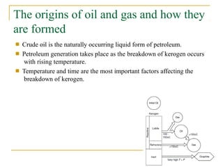
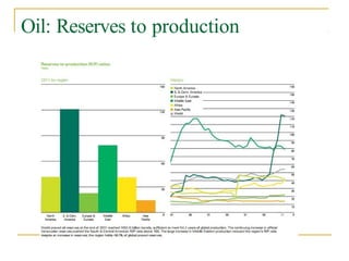
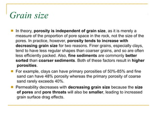
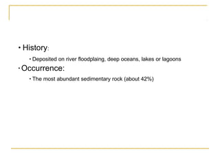
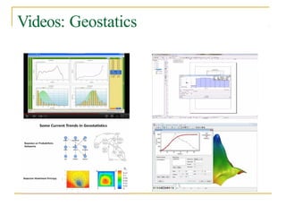
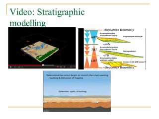
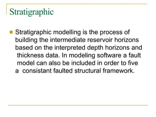
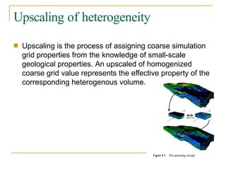
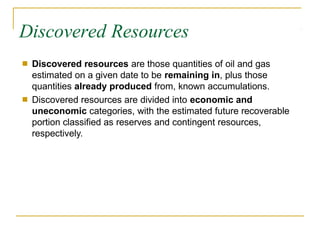
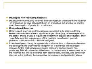
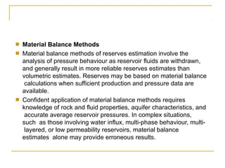
![■ The Hubbert peak theory is based on the observation
that the amount of oil under the ground in any region
is finite, therefore the rate of discovery which
initially increases quickly must reach a maximum and
decline. In the US, oil extraction followed the
discovery curve after a time lag of 32 to 35 years.[1][2]
The theory is named after American geophysicist
M. King Hubbert, who created a method of modeling
the production curve given an assumed ultimate
recovery volume.](https://image.slidesharecdn.com/sodapdf-converted7-240813182559-741230f0/85/Reservoir-Modeling-and-charactarization-pptx-17-320.jpg)
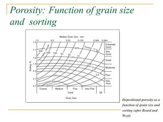
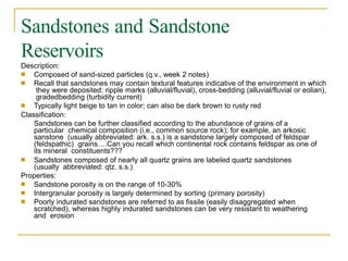
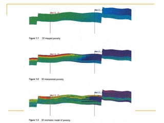
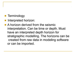
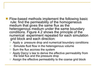
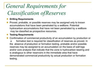
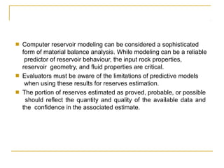
![• Components that constitute natural gas
■ Natural gas is a naturally occurring gas mixture consisting primarily of
methane, typically with 0–20% higher hydrocarbons[1] (primarily ethane).
It is found associated with other hydrocarbon fuel, in coal beds, as
methane clathrates, and is an important fuel source and a major
feedstock for fertilizers.
Most natural gas is created by two mechanisms: biogenic and
thermogenic. Biogenic gas is created by methanogenic organisms in
marshes, bogs, landfills, and shallow sediments. Deeper in the earth, at
greater temperature and pressure, thermogenic gas is created from
buried organic material.[2]
Before natural gas can be used as a fuel, it must undergo processing to
remove almost all materials other than methane. The by-products of
that processing include ethane, propane, butanes, pentanes, and
higher molecular weight hydrocarbons, elemental sulfur, carbon dioxide
, water vapor, and sometimes helium and nitrogen.
Natural gas is often informally referred to as simply gas, especially
when compared to other energy sources such as oil or coal.
■
■
■](https://image.slidesharecdn.com/sodapdf-converted7-240813182559-741230f0/85/Reservoir-Modeling-and-charactarization-pptx-20-320.jpg)


![the INTRODUCTION_TO_OIL&GAS_Recent[1].ppt](https://cdn.slidesharecdn.com/ss_thumbnails/introductiontooilgasrecent1-251206200220-5afcef01-thumbnail.jpg?width=640&height=640&fit=bounds)


