The document discusses several previous studies conducted by Amity University experts related to agriculture and remote sensing. One study analyzed big data pattern mining using graphs to identify clusters and frequent subgraphs. Another used thermal imaging and hyperspectral remote sensing to monitor crop water deficit stress in rice genotypes and identify optimal wavelengths. A third compared modeling approaches to monitor water deficit stress in rice using hyperspectral data and measured relative water content. The studies demonstrated applications of machine learning, remote sensing, and hyperspectral data for agricultural monitoring and analysis.


![14 | P a g e
Name of Study
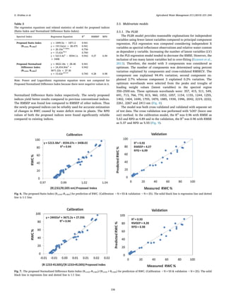
Name of study
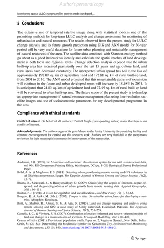
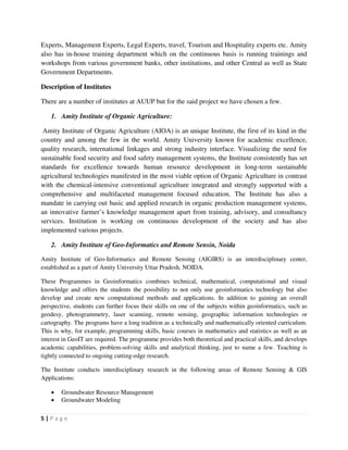
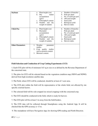
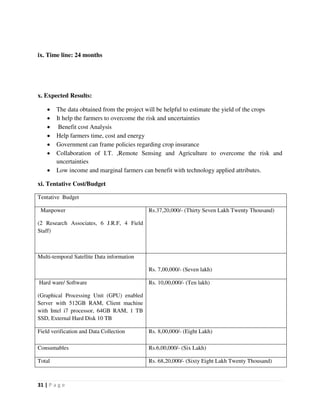
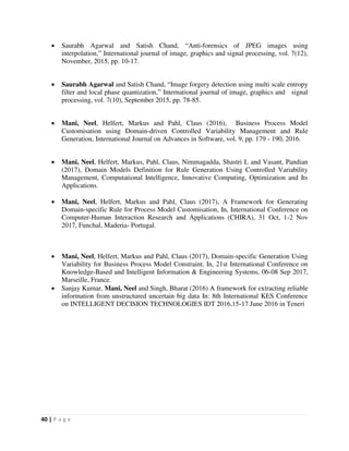
Methods of LeafArea for Stevia rebaudiana (Bert.) Bertoni
Leaf area is a valuable index for evaluating growth and development of sweet herb
Stevia [Stevia rebaudiana (Bert.) Bertoni]. A simple methodology was developed
during 2006 to estimate the leaf area through Leaf Area Distribution Pattern
(LADP) and regression equations. Plant height, leaf height as well as the length and
breadth of all the measurable leaves were measured and their area was measured
through Area meter (AM 300) for a six month old crop of Stevia. A leaf area
coefficient of 0.548 was found to fit for the linear equation without intercept.
LADP was prepared with relative leaf height and relative leaf area. Based on the
adjusted second order polynomial equation of LADP, the relative leaf height of
plants representing the mean leaf area was ascertained and a regression equation
was obtained to calculate the total leaf area of the plant. The results were validated
with 3, 4 and 5 months old crops as well as with another accession. Different
combinations of prediction equations were obtained from length and breadth of all
leaves and a simplest equation i.e, linear equation was used to predict the leaf area.
A non-destructive methodology for estimating leaf area of Stevia based on linear
measurement was developed in this study.
SIMULATION AND VALIDATION OF CERES-MAIZE AND CERES-
BARLEY MODELS
Investigations were carried out for determination of genotypic co-efficients of
important varieties of maize and barley, simulation and validation of CERES-Maize
and CERES- Barley crop models for growth, yield and yield attributes, and working
out simulation-guided management practices for yield maximization of both the
crops. Field experiments comprising of four dates of sowing (June 1, June 10, June
20 and June 30) and four varieties (KH 9451, KH 5991, early composite and local)
of maize and four dates of sowing (October 10, November 1, November 20 and
December 10) and three varieties (Dolma, Sonu and HBL-113) of barley were
conducted during Kharif 2002 to Rabi 2004-05 in split plot design. Observations on
development stages, dry matter accumulation (leaves, stem and grains) at 15 days
interval, yield attributes, yield (grains, stover/straw and biological), nitrogen
content and uptake were recorded. Genotypic coefficients of important
recommended varieties of maize and barley were worked out. CERES-Maize model
successfully simulated phenological stages, yield attributes (except test weight),
yield and also N uptake, but failed to simulate accurately dry matter accumulation
in different plant parts at different growth periods. CERES-Barley model also
successfully simulated phenological stages, yield attributes and grain yield, but
failed to simulate straw yield, dry matter accumulation in different plant parts at
different growth periods and N content and uptake. Both the models were validated
with fair degree of accuracy. Simulation guided management practices were
worked out under potential production and resource limiting situations. In case of
maize, best time of sowing of both hybrids(KH 9451, KH 5991) was worked out to
be last week of April. While for early composite, first week of May proved
advantageous and for local second fortnight of April. The best schedule of N
application was 60 kg /ha at sowing time and 30 kg/ha at knee high stage for all
varieties except for local where it was 60 kg /ha at sowing and 30kg/ha at knee high
stage and 30 kg/ha at silking. In case of barley, best time of sowing for Dolma and](https://image.slidesharecdn.com/researchproposalamityuniversity-191017061352/85/Research-proposal-amity-university-14-320.jpg)


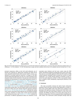
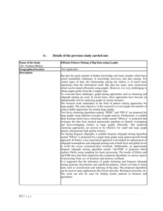
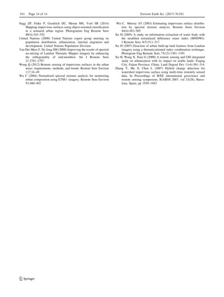
![the regular monitoring and assessment are a prerequisite to
understand the water quality. Many governments are now
seeing other approaches in response to increasing aware-
ness of degrading lake water resources and growing con-
cern over the significant fiscal burden of agricultural
subsidies.
Earth observation data sets, e.g., satellite images, are
quite useful, which could be used for synoptic representa-
tion of any area (Srivastava et al. 2010). Land use/land
cover change (LULCC) quantification is one of the major
application of earth observation data sets, and it is impor-
tant for assessing global environmental change processes
and helps in making new policies and optimizing the
maximum use of natural resources in sustainable manners
(Srivastava et al. 2012). The land use/land cover
(LULC) types, such as agricultural land and urban area, are
associated with human activities that often affect the water
quality and change the aquatic ecological environment;
hence, monitoring spatial–temporal changes is essential to
understand the driving factors which influence the water
quality of any area. Amin et al. (2014) and Mishra and
Garg (2011) has did research on lake of India by implying
the satellite data.
According to Singh et al. (2015), the concept of water
quality to categorize water according to its degree of purity
or pollution dated back to year 1848. Around the same
time, the importance of water quality to public health was
recognized in the UK (Snow 1856). Water Quality Index
(WQI) methodologies have been developed to provide
single number that expresses the overall water quality at a
certain location and time, based on several water quality
parameters (Parmar and Bhardwaj 2013; Vasanthavigar
et al. 2010; Avvannavar and Shrihari 2008; Singh et al.
2015) and can be used to provide the overall summaries of
water quality on a scientific basis. Parmer and Bhardwaj
(2013) have applied WQI and fractal dimension approach
to study the water of Harike lake on the confluence of Beas
and Sutlej rivers of Punjab (India). Many researchers have
discussed the importance and applicability of WQI for
water characterization (Couillard and Lefebvre 1985;
House and Newsome 1989; Bordalo et al. 2001; Smith
1989; Swamee Tyagi 2000; Sanchez et al. 2007).
In combination with remote sensing water quality, the
use of multivariate statistical techniques offers a detailed
understanding of water quality parameters and possible
factors that influence the water quality behavior (Srivastava
et al. 2012). Principal component analysis (PCA) and factor
analysis (FA) offer a valuable tool for consistent, reliable,
effective management of water resources (Srivastava et al.
2012; Singh et al. 2009, 2013d, 2015). Many authors in past
have used multivariate statistical techniques to characterize
and evaluate surface and groundwater quality and have
found it interesting for studying the variations caused by
geogenic and anthropogenic factors (Shrestha and Kazama
2007; Singh et al. 2005). For understanding the lake water
quality, multivariate statistical techniques integrated with
remote sensing, and WQI (Srivastava et al. 2012) could be
used for identification of the possible factor/sources that
influences urban lake water quality.
As the study area occupied by hard basaltic terrain and
groundwater resource are limited. Hence, largely the water
supply in urban areas setteled at hard rock terrain depends
on lake water too for drinking and small scale industrial
purposes. The water supply of bhopal urban area mainly
depends on the Bhopal lake for drinking, irrigation and
small scale industries.
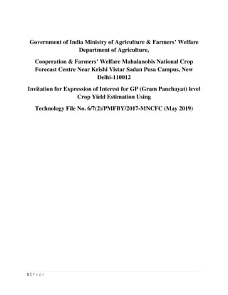
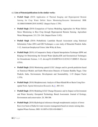
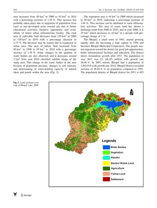
The specific objective of this research was focused on to
quantify the historical changes in LULC using satellite data
sets and its probable impact on the lake water quality with
integration of statistical techniques to know the pollution
status of Bhopal lake and to categorize lake water by WQI
method. The findings of the study will be useful for the
restoration of Bhopal lake.
Materials and methods
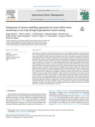
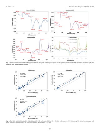
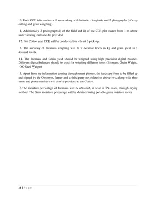
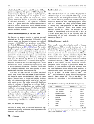
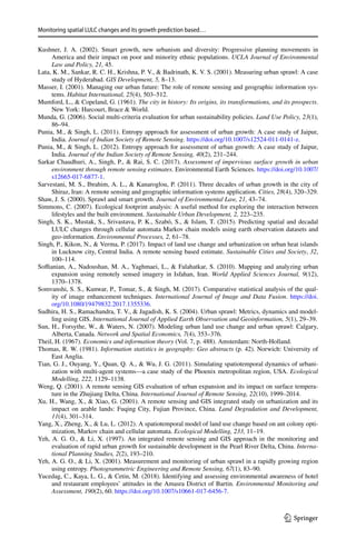
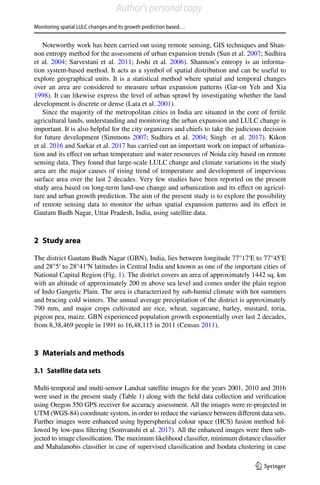
Description of study area
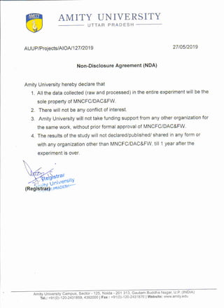
District Bhopal [latitudes 20°100
–23°200
N and longitudes
77°150
–77°250
E (Fig. 1)] is the capital city of the state of
Madhya Pradesh, India. Upper lake commonly known as
Bhoj wetland is the main lake of the city and provides
water to the dwellers. The lake surrounded by natural
landscape, settlements and agricultural fields. The average
annual rainfall is 1270 mm. The southern part of the city
receives more rainfall than northern part of the city. The
maximum rainfall takes place during the month of July.
The area is drained by small drains which are lastly
contributing water to the river Betwa in the downstream.
Bhopal has been growing at a fast rate due to urban
development and industrialization, in search of better
facilities and for educational purposes. The major part of
the city is covered by Vindhyan hills and by basaltic
Deccan trap. The Deccan trap covers almost one-third of
the area followed by Vindhyan sandstone (Singh and Singh
2012). In Deccan trap basalts, aquifer is encountered at
shallow depth and in Vindhyan sandstone depth ranges
more than 150 meter below ground level (mbgl). The water
supply to Bhopal city mainly comes from surface water
bodies and small amount by groundwater. Nowadays, a
number of boreholes/tube wells are drilled in the area
without consideration of hydrological status of the aquifer
formation to meet the water requirement, and this unaware
drilling has also led to the declining trend of water level
and also failure of well in successive years. Upper lake is a
446 Int. J. Environ. Sci. Technol. (2016) 13:445–456
123](https://image.slidesharecdn.com/researchproposalamityuniversity-191017061352/85/Research-proposal-amity-university-45-320.jpg)
![for errors or other sources of variation, i the sample num-
ber, j the variable number and m the total number of
factors.
Results and discussion
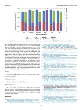
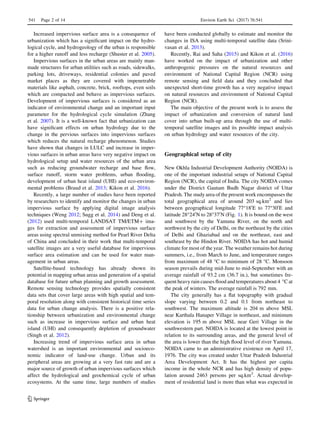
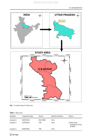
Hydrochemistry of lake water
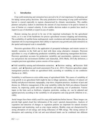
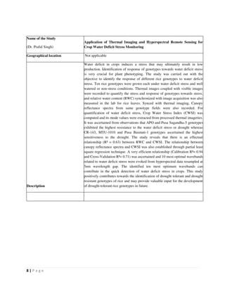
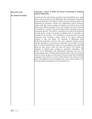
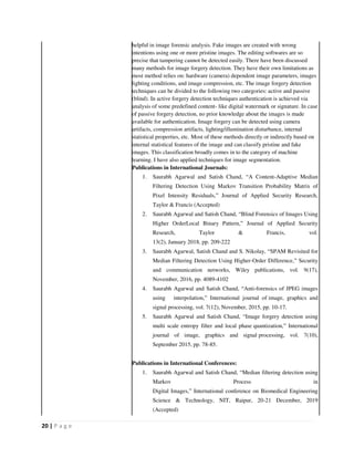
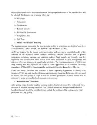
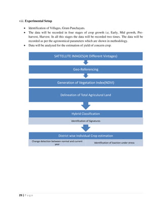
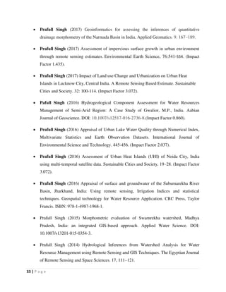
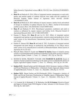
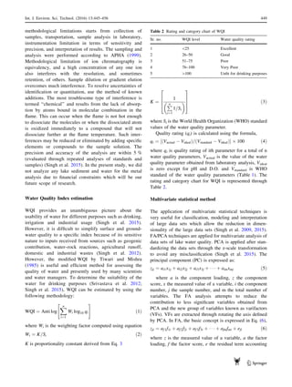
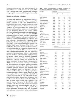
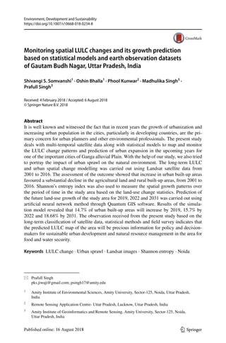
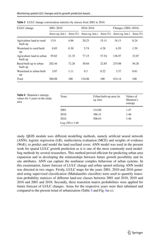
The descriptive statistics of 12 physicochemical parameters
at the 15 locations are summarized in Table 3. The average
value of total alkalinity 78.67, 60.07 and 57.20 was
observed during the pre-monsoon, monsoon and post-
monsoon seasons. Carbonate alkalinity average value was
13.19, 11.80 and 6.80, and bicarbonate alkalinity was
65.49, 49.43 and 50.96; total hardness average value was
85.25, 94.77 and 89.84, calcium hardness was 60.12, 67.10
and 68.58 and magnesium hardness was 25.14, 27.67 and
21.27 in the pre-monsoon, monsoon and post-monsoon
seasons, respectively. Calcium and magnesium are an
essential nutrient that is required by all living organisms.
Calcium and magnesium are entirely derived from rock
weathering. The sources of Ca mainly are carbonate rocks
containing calcite (CaCO3) and dolomite [(CaMg(CO3)2],
with a lesser proportion derived from Ca-silicate minerals.
Calcium is usually one of the most important contributors
to hardness. The average value of Ca was 25.25, 28.18 and
28.80, magnesium 6.11, 6.72 and 5.17 in the pre-monsoon,
monsoon and post-monsoon seasons, respectively.
Chloride is extremely mobile and very much soluble in
surface water. The main geogenic sources of chloride are
sea salt and dissolution of halite (NaCl) in bedded evap-
orites or dispersed in shales, and anthropogenic sources are
domestic and industrial sewage, mining, and road salt
runoff. The average value of chloride was 6.13, 21.03 and
19.35 in the all three seasons, respectively.
Phosphorus is a vital and often limiting nutrient. The
most common minerals are apatite, which is calcium
phosphate with variable amounts of hydroxyl-, chloro-, or
fluoro-apatite and various impurities. Some other phos-
phate minerals contain aluminum or iron. The anthro-
pogenic sources of phosphorus are domestic sewage, as the
element is essential in metabolism, industrial sewage and
household detergents. Phosphates and nitrates are the major
cause of eutrophication problem in lakes. The average
values of phosphate were 1.05, 0.76 and 0.62, total phos-
phorous was 1.62, 1.91, and 1.80, organic phosphorous was
1.13, 1.16 and 1.18 and nitrate was 0.73, 0.73 and 0.64 in
the pre-monsoon, monsoon and post-monsoon season,
respectively. Aqueous geochemistry behavior of nitrogen is
strongly influenced by the vital importance of the element
in plants and animal nutrition. The anthropogenic sources
of nitrate in surface water are runoff from the agriculture
field, and leachates from the landfill sites. The BOD was
3.83, 4.83 and 4.42, and COD was 29.60, 21.06 and 15.73
in the pre-monsoon, monsoon and post-monsoon season,
respectively. The development activity and expansion of
the city leading to discharge of waste water in the upper
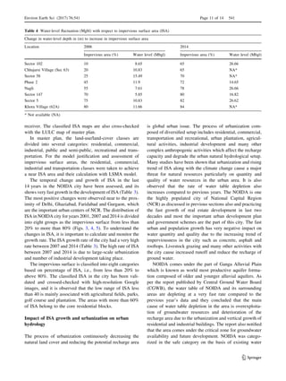
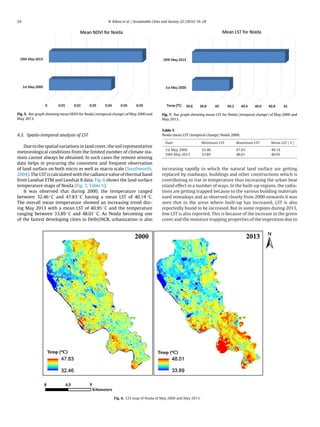
Table 3 Physicochemical properties of lake water samples during the three seasons (all the parameters units are in mg/l)
Parameters Pre-monsoon Monsoon Post-monsoon
Max Min Avg Std Max Min Avg Std Max Min Avg Std
Total alkalinity 129.60 61.60 78.67 18.55 98.00 49.00 60.07 12.03 78.67 46.67 57.20 7.50
Carbonate alkalinity 17.60 7.00 13.19 2.95 16.67 7.00 11.80 2.78 11.33 4.00 6.80 2.30
Bicarbonate alkalinity 118.40 46.00 65.49 19.84 94.50 36.50 49.43 13.99 76.00 42.67 50.96 8.06
Total hardness 146.00 74.80 85.25 17.53 155.50 79.50 94.77 18.13 116.67 62.67 89.84 17.23
Ca hardness 105.00 51.66 60.12 13.26 122.85 55.65 67.10 16.66 104.30 55.30 68.58 12.99
Mg hardness 41.00 18.56 25.14 5.90 33.73 19.48 27.67 5.27 42.07 7.37 21.27 10.38
Calcium content 44.10 21.70 25.25 5.57 51.60 23.37 28.18 7.00 43.81 23.23 28.80 5.46
Magnesium content 9.96 4.51 6.11 1.43 8.20 4.73 6.72 1.28 10.22 1.79 5.17 2.52
Chloride 31.17 12.99 16.13 4.27 35.21 16.23 21.03 4.54 27.64 15.65 19.35 2.83
Phosphate 3.19 0.49 1.05 0.68 3.14 0.18 0.76 0.74 3.06 0.12 0.62 0.72
Total phosphorus 3.56 0.94 1.62 0.71 4.05 1.15 1.91 0.8 3.93 1.03 1.80 0.80
Organic phosphorus 2.31 0.43 1.13 0.47 2.33 0.45 1.16 0.47 2.66 0.55 1.18 0.51
Nitrate 1.88 0.11 0.73 0.46 1.86 0.09 0.73 0.45 1.77 0.07 0.64 0.46
BOD 4.88 3.08 3.83 0.56 11.60 3.40 4.83 1.94 10.00 2.00 4.42 2.60
COD 44.80 23.20 29.60 4.70 35.00 16.06 21 4.75 30.67 12.00 15.73 4.37
450 Int. J. Environ. Sci. Technol. (2016) 13:445–456
123](https://image.slidesharecdn.com/researchproposalamityuniversity-191017061352/85/Research-proposal-amity-university-49-320.jpg)

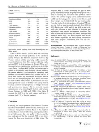
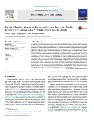
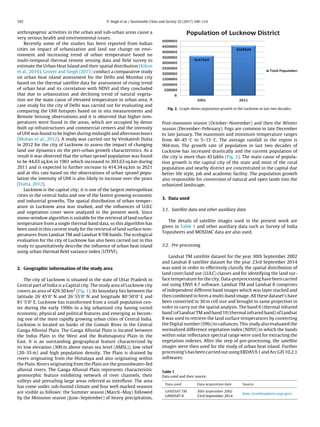
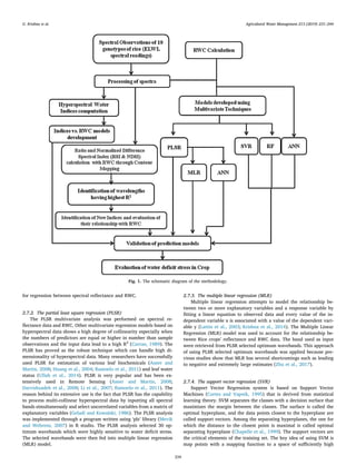
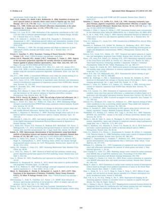
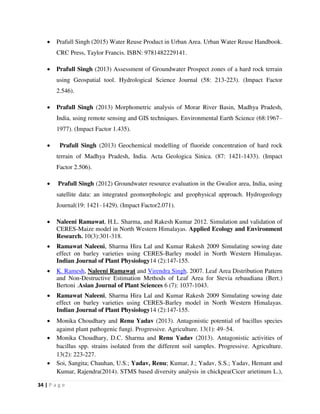
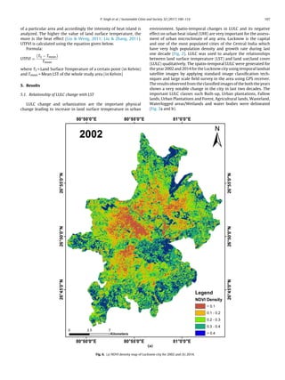
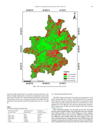
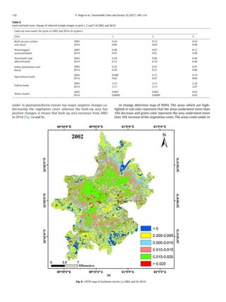
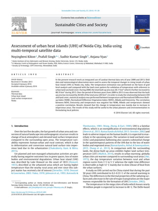
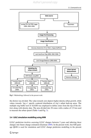
![P. Singh et al. / Sustainable Cities and Society 32 (2017) 100–114 103
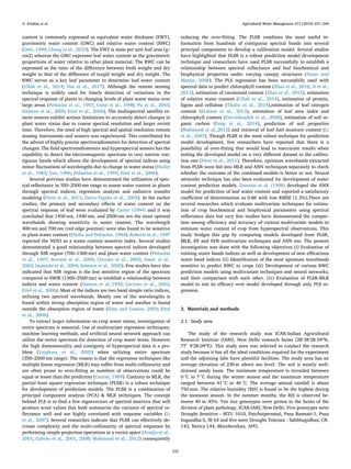
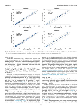
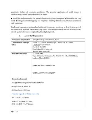
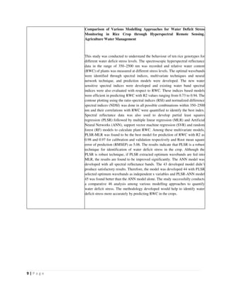
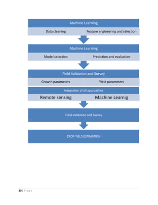
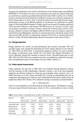
3.3. Image classification
Supervised classification scheme has been used for the pro-
cess of image classification in which training sets were selected
for image classification using Maximum Likelihood classifier
(MLC), a statistical decision in which the pixels are assigned
based on the class of maximum probability. Image classifica-
tion was used to define the Land use/Land cover types into
seven classes, namely, Built up, Water logged areas/Wetlands,
Wasteland (Salt affected land), Urban Plantations and Forest,
Agricultural lands, Fallow lands and Water bodies have been
categorized. As described by Lillesand, Kiefer, and Chipman
(2014), confusion matrix was also generated from the classified
image and signature file for the accuracy assessment. Overall
accuracy of LULC map was 88.38% and Kappa coefficient was
0.832.
4. Methodology
4.1. Mono-window algorithm for the retrieval of LST
In this study, land surface temperature (LST) of Lucknow city
was estimated from the thermal infrared bands of Landsat satel-
lite data’s using the mono-window algorithm proposed by Liu and
Weng (2011), Liu and Zhang (2011) and Qin, Zhang, Amon, and
Pedro (2001). This algorithm is carried out using three main param-
eters, namely, transmittance, emissivity and mean atmospheric
temperature. TIR band 6 of Landsat TM and TIR band 10 of Landsat
8 records the radiation with spectral range ranging from 10.40 to
12.50 for Landsat TM data’s and 10.60 to 11.19 for Landsat 8 data’s.
Formula:
Tc = {a(1 − C − D) + [b(1 − C − D) + C + D]Ti − D ∗ Ta}/C
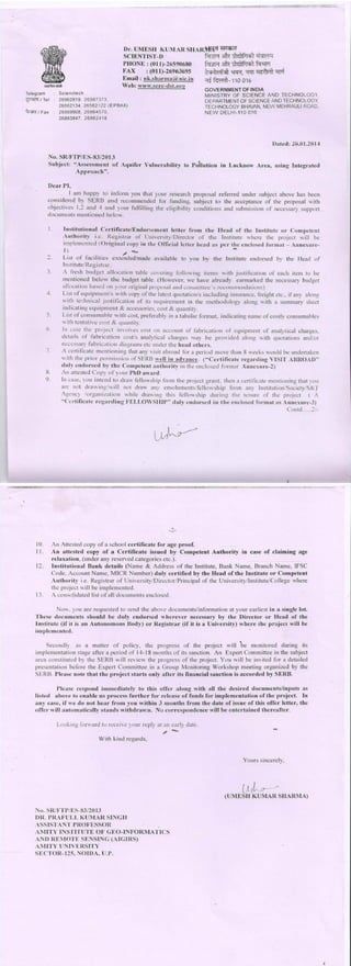
Fig. 3. (a) Land use/land cover map of Lucknow city for 2002 and (b) 2014.](https://image.slidesharecdn.com/researchproposalamityuniversity-191017061352/85/Research-proposal-amity-university-59-320.jpg)
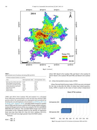


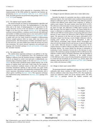
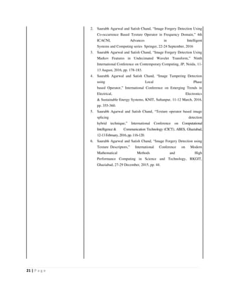
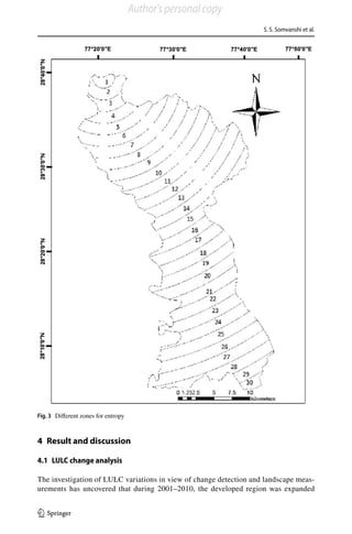
![Monitoring spatial LULC changes and its growth prediction based…
1 3
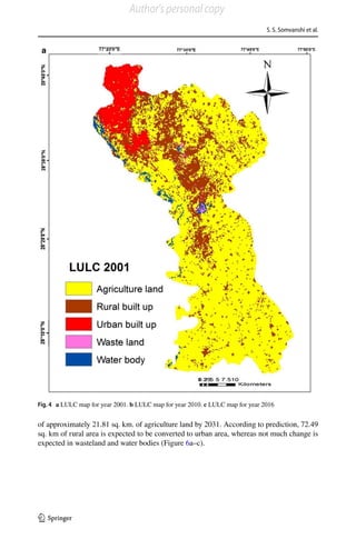
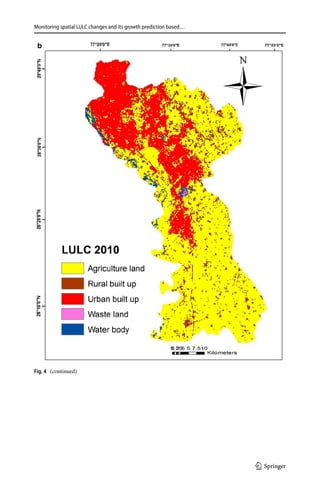
by 271.43 sq. km. The LULC cover change in the area clearly indicates that in last 2
decades the growth of urbanization increases drastically and the major changes were
observed in conversion of agricultural land into urban and rural area in urban built up.
The urban built-up area in 2001 was 114.88 sq. km, and agriculture area was 1015.53
sq. km; however, in 2010, the urban built-up increased to 386.31 sq. km and agricul-
ture land decreased to 931.53 sq. km (Fig. 4a–c). It is also observed that large-scale
change in rural area into dense built-up land due to the growth in construction projects.
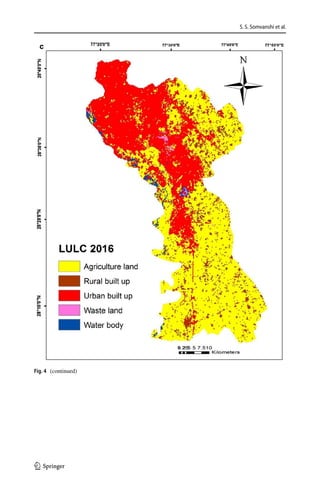
Another important LULC change was observed between second phase of development
from 2010 to 2016 in urban built land and its increase up to 120.32 sq. km in last
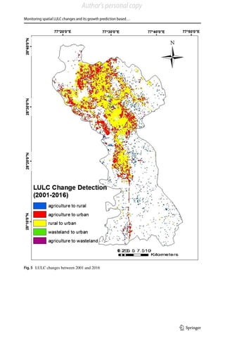
6 years (Table 2). It is observed that more than 34.13 sq. km of agricultural land has
been converted to the urban built-up area in the last 16 years and most of the urbaniza-
tion has taken place on agricultural and open lands (Fig. 5). The unexpected expan-
sion of urban developed regions not just brought about the discontinuity of crop land,
but also decreased the productivity of crop and groundwater resource due to reduction
in surface recharge area. Ultimately, it caused a serious problem for food and water
security.
4.2 Urban sprawl analysis
The Shannon’s entropy (Hn) was measured for the assessment of urban environment to
examine the degree of dispersion or compactness of the spatial growth of the city. The
highest range of Shannon’s entropy [Loge (30)] is 1.48, and entropy results obtained from
three study periods were 1.47, 1.46 and 1.46, respectively (Table 4). The values observed
for all the 3 years were towards 1.48 (log 30). The entropy results revealed that there was
urban expansion in the area exponentially since 2001 in south-east direction. The rate of
overall expansion of the area has very negative impact on ecological, environmental, eco-
nomic and social aspect (Mumford and Copeland 1961; Munda 2006; Bhatta et al. 2009).
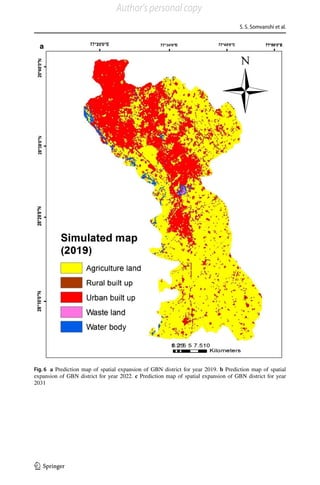
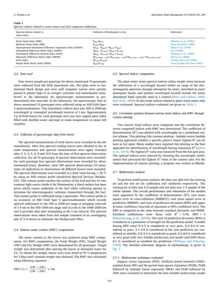
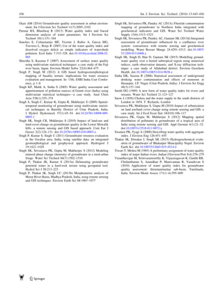
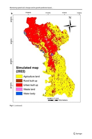
4.3 LULC prediction modelling
LULC maps of 2001 and 2010 were identified as input data to predict 2019 land use, 2010
and 2016 maps were used as input to predict 2022, and LULC maps of 2001 and 2016
were used as input data to predict 2031. According to the analysis during the study, the
land-use change will reach to extreme in 2019, 2022 and 2031 and urban area will increase
and occupy 40.29%, 40.65% and 41.69% of the district’s area, respectively (Table 5). How-
ever, cultivated land will decrease, respectively, year after year, resulting in potential loss
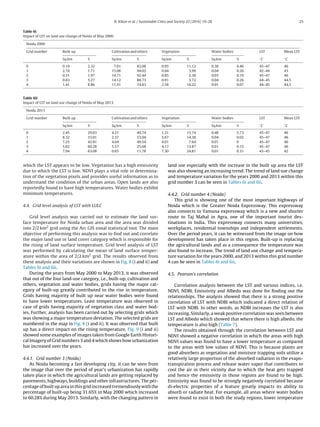
Table 5 Estimation of urban sprawl and LULC changes for 2019, 2022 and 2031
Classes 2019 2022 2031
Area (sq. km.) Area (%) Area (sq. km.) Area (%) Area (sq. km.) Area (%)
Agriculture land 818.94 56.6 814.24 56.46 801.61 55.59
Rural built up 18.31 1.26 18.12 1.25 15.70 1.08
Urban built up 581.12 40.29 586.18 40.65 601.23 41.69
Wasteland 1.39 0.09 1.37 0.09 1.25 0.08
Water body 22.24 1.54 22.09 1.53 22.21 1.54](https://image.slidesharecdn.com/researchproposalamityuniversity-191017061352/85/Research-proposal-amity-university-79-320.jpg)


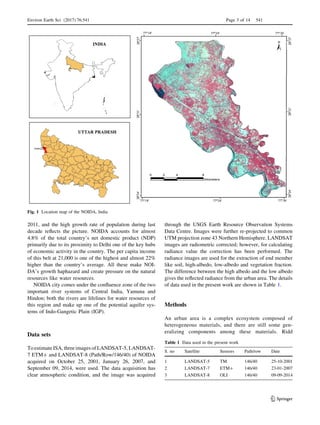
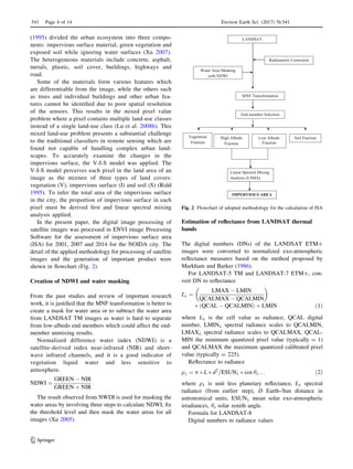

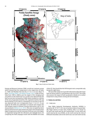
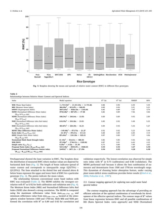
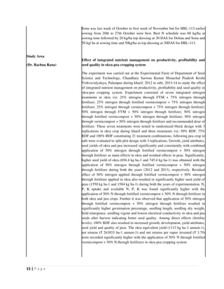
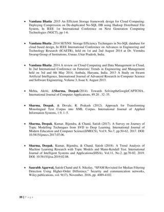
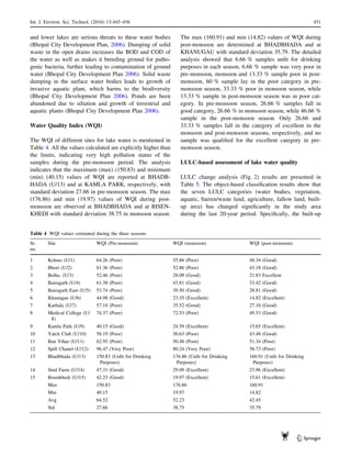
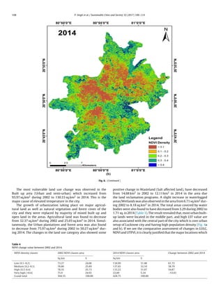
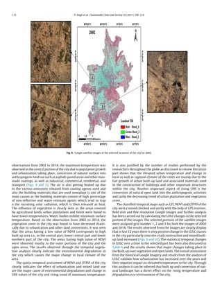
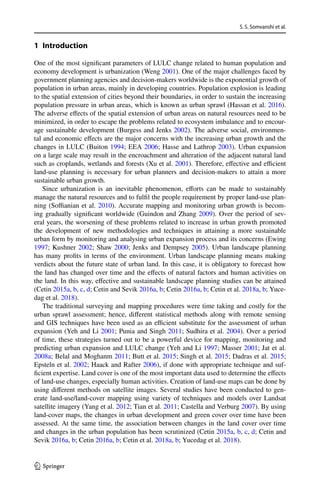
![N. Kikon et al. / Sustainable Cities and Society 22 (2016) 19–28 21
Table 1
Data used and their source.
Data used Data acquisition date Data source
LANDSAT ETM 1st May 2000 http://earthexplorer.
usgs.gov/LANDSAT 8 29th May 2013
the Hindon River. Noida is spread over an area of 203 km2, and has a
population of around 0.64 million. Noida has hot and humid climate
for most of the year. The weather remains hot during summers, i.e.,
from March to June, and temperature ranges from maximum of
48 ◦C to minimum of 28 ◦C. Monsoon season prevails during mid-
June to mid-September with an average rainfall of 93.2 cm (36.7 in.),
but sometimes frequent heavy rain causes flood. Temperatures fall
down to as low as 3 to 4 ◦C at the peak of winters. Noida also has
fog and smog in winters (http://noida.trade/cityClimatesection).
Due to a rapid industrialization and urbanization and infrastructure
development in Delhi and Noida, develops ecological imbalance
due to exploitation and overuse of environmental resources which
have adverse effect as UHI (Fig. 1).
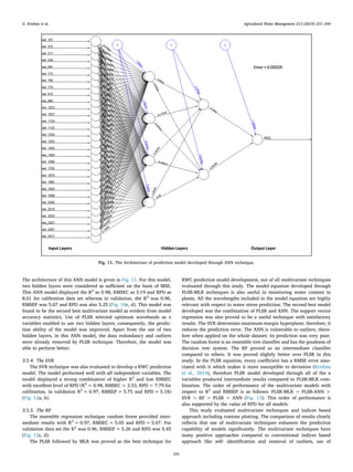
2.2. Data used
2.2.1. Satellite data and other auxiliary data
The details of satellite images are given in Table 1 and other
auxiliary data as Survey of India Toposheets and MOSDAC data has
been used in the study.
2.2.2. Preprocessing
Satellite data pre-processing was carried out using ENVI 4.7
software. Each Landsat ETM and Landsat 8 data consisted of inde-
pendent distinct band images which was first layer stacked and
combined into a multi-band image. These images have a spatial res-
olution of 30 m per pixel. In this study the band 6 (thermal infrared
band) of ETM and band 10 (thermal infrared band) of Landsat 8 was
used to retrieve the LST by converting the Digital number (DNs)
into radiances. The bands within solar reflectance spectral range
were used for extracting the vegetation and built up indexes. After
pre-processing, the images of the study area were used for the anal-
ysis of UHI study. Further, processing has been carried out on Arc
GIS 10.2.1 software. Statistical analysis was carried out using SPSS
software.
3. Methodology used
3.1. Mono-window algorithm for the retrieval of LST
Mono-window algorithm proposed by Qin, Karnieli, and
Berliner (2001), for the retrieval of LST from Landsat TM 6 data have
been used in the study (Liu Zhang, 2011). This algorithm necessi-
tates three main parameters – emissivity, transmittance and mean
atmospheric temperature. Band 6 of Landsat ETM and band 10 of
Landsat 8 records the radiation with spectral range from 10.40 to
12.50 m for Landsat ETM and 10.60 to 11.19 m for Landsat 8. The
following expression is given below as Eq. (1):
Ts = {a(1 − C − D) + [b(1 − C − D) + C + D]Ti − D ∗ Ta}/C (1)
where a = −67.355351, b = 0.4558606, C = εi * i, D = (1 − i)
[1 + (1 − εi) * i), εi = emissivity and i = transmissivity.
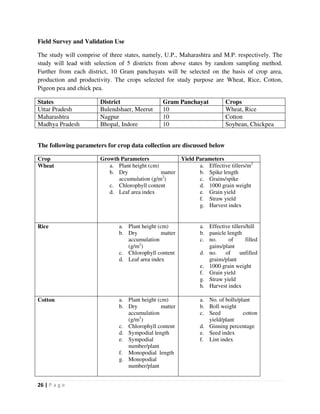
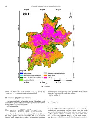
3.1.1. Conversion of digital numbers to radiance
In order to convert the DN data of band 6 of Landsat ETM and
band 10 of Landsat 8 into spectral radiance Eqs. (2) and (3) can be
written in band math of ENVI 4.7 as:
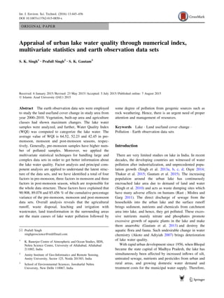
Fig. 2. NASA webpage for atmospheric correction.
Source: atmcorr.gsfc.nasa.gov/
(a) For Landsat ETM
CVR1 =
(LMAX − LMIN )
(QCALMAX − QCALMIN) ∗ (QCAL − QCALMIN) + LMIN
(2)
where CVR1 is the cell value as radiance, QCAL = Digital Number,
LMIN = spectral radiance scales to QCALMIN, LMAX = spectral
radiance scales to QCALMAX, QCALMIN = the minimum quan-
tized calibrated pixel value (typically 1) and QCALMAX = the
maximum quantized calibrated pixel value (typically 255).
(b) For Landsat 8
L = MLQCal + AL (3)
where L = TOA spectral radiance (Watts/(m2 × srad × m)),
ML = band-specific multiplicative rescaling factor from the
metadata (RADIANCE MULT BAND x, where x is the band num-
ber), AL = Band-specific additive rescaling factor from the
metadata (RADIANCE ADD BAND x, where x is the band num-
ber), QCal = quantized and calibrated standard product pixel
values (DN). These useful values can all be obtained from the
meta-data file of the satellite image data.
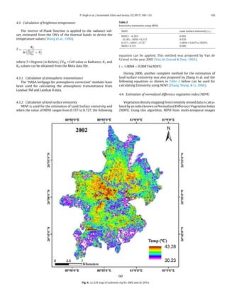
3.1.2. Calculation of brightness temperature
Once the radiance values have been calculated using the DNs of
the thermal bands, the inverse of the Plank function is applied to
derive the temperature values (Wang et al., 1990) expressed as Eq.
(4).
T =
K2
ln
K1×ε
CVR1
+ 1
(4)
where T = degrees (in K), CVR1 = cell value as radiance. K1 and K2
values can be obtained from the meta-data file.
3.1.3. Calculation of atmospheric transmittance
The atmospheric transmittance for Landsat ETM and Landsat
8 data was calculated using the “NASA webpage for atmospheric
correction” module (Fig. 2).](https://image.slidesharecdn.com/researchproposalamityuniversity-191017061352/85/Research-proposal-amity-university-106-320.jpg)


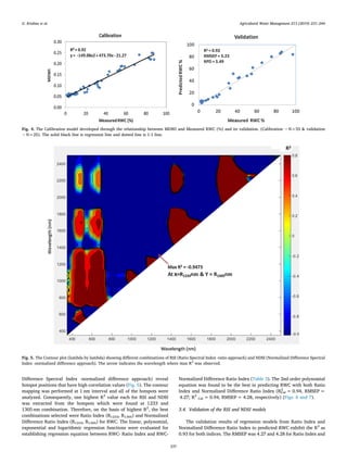
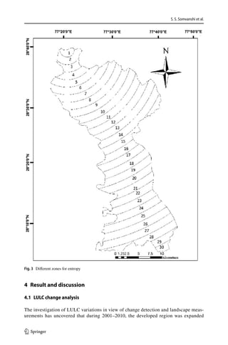
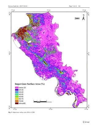
![Monitoring spatial LULC changes and its growth prediction based…
1 3
by 271.43 sq. km. The LULC cover change in the area clearly indicates that in last 2
decades the growth of urbanization increases drastically and the major changes were
observed in conversion of agricultural land into urban and rural area in urban built up.
The urban built-up area in 2001 was 114.88 sq. km, and agriculture area was 1015.53
sq. km; however, in 2010, the urban built-up increased to 386.31 sq. km and agricul-
ture land decreased to 931.53 sq. km (Fig. 4a–c). It is also observed that large-scale
change in rural area into dense built-up land due to the growth in construction projects.
Another important LULC change was observed between second phase of development
from 2010 to 2016 in urban built land and its increase up to 120.32 sq. km in last
6 years (Table 2). It is observed that more than 34.13 sq. km of agricultural land has
been converted to the urban built-up area in the last 16 years and most of the urbaniza-
tion has taken place on agricultural and open lands (Fig. 5). The unexpected expan-
sion of urban developed regions not just brought about the discontinuity of crop land,
but also decreased the productivity of crop and groundwater resource due to reduction
in surface recharge area. Ultimately, it caused a serious problem for food and water
security.
4.2 Urban sprawl analysis
The Shannon’s entropy (Hn) was measured for the assessment of urban environment to
examine the degree of dispersion or compactness of the spatial growth of the city. The
highest range of Shannon’s entropy [Loge (30)] is 1.48, and entropy results obtained from
three study periods were 1.47, 1.46 and 1.46, respectively (Table 4). The values observed
for all the 3 years were towards 1.48 (log 30). The entropy results revealed that there was
urban expansion in the area exponentially since 2001 in south-east direction. The rate of
overall expansion of the area has very negative impact on ecological, environmental, eco-
nomic and social aspect (Mumford and Copeland 1961; Munda 2006; Bhatta et al. 2009).
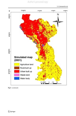
4.3 LULC prediction modelling
LULC maps of 2001 and 2010 were identified as input data to predict 2019 land use, 2010
and 2016 maps were used as input to predict 2022, and LULC maps of 2001 and 2016
were used as input data to predict 2031. According to the analysis during the study, the
land-use change will reach to extreme in 2019, 2022 and 2031 and urban area will increase
and occupy 40.29%, 40.65% and 41.69% of the district’s area, respectively (Table 5). How-
ever, cultivated land will decrease, respectively, year after year, resulting in potential loss
Table 5 Estimation of urban sprawl and LULC changes for 2019, 2022 and 2031
Classes 2019 2022 2031
Area (sq. km.) Area (%) Area (sq. km.) Area (%) Area (sq. km.) Area (%)
Agriculture land 818.94 56.6 814.24 56.46 801.61 55.59
Rural built up 18.31 1.26 18.12 1.25 15.70 1.08
Urban built up 581.12 40.29 586.18 40.65 601.23 41.69
Wasteland 1.39 0.09 1.37 0.09 1.25 0.08
Water body 22.24 1.54 22.09 1.53 22.21 1.54
Author's personal copy](https://image.slidesharecdn.com/researchproposalamityuniversity-191017061352/85/Research-proposal-amity-university-124-320.jpg)