This document analyzes factors affecting housing prices in Boston suburbs using linear regression. Exploratory data analysis identifies relationships between variables and transforms some to better fit linear models. Variable selection methods identify the best predictors. A customized model with transformed variables and interaction terms outperforms other models with an adjusted R-squared of 0.85. While CART predicts better than linear regression alone, the customized linear model incorporates more information from exploratory analysis to perform best overall.

1. BOSTON HOUSING DATA
A Comprehensive Regression Analysis
Ravish Kalra
Graduate Student, Business Analytics
University of Cincinnati

2. Table of Contents
Executive Summary - Boston Housing Data.................................................................................................2
Boston Housing Data.....................................................................................................................................3
Introduction ..............................................................................................................................................3
Exploratory Data Analysis .........................................................................................................................3
Variable Selection and Modelling .............................................................................................................7
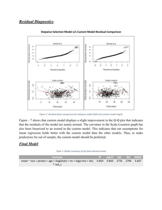
Residual Diagnostics .................................................................................................................................9
Final Model ...............................................................................................................................................9
Comparison with CART ...........................................................................................................................10
Executive Summary - Boston Housing Data
This report provides an analysis and evaluation of the factors affecting the median value of the
owner occupied homes in the suburbs of Boston. The in-built data set of Boston Housing Data is
used for this analysis and various factors about the structural quality, neighbourhood,
accessibility and air pollution such as per capita crime rate by town, proportion of non-retail
business acres per town, index of accessibility to radial highways etc are taken into account for
this study.
Methods of analysis include (but not limited to) summary statistics and visualization of the
distribution of the variables, finding correlation between variables and conducting linear
regression on the data.
Further, various variable selection methods like Best Subset, Stepwise Selection and LASSO was
performed to come up with the best linear regresssion model to predict the median value of the
owner occupied homes. These models were then compared with a custom model designed after
including all the analysis from the initial exploration.
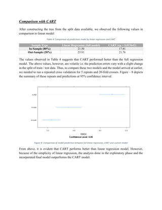
Finally, a comprehensive comparison was made between linear regression and CART to predict
the median price values after supplying the same data. The results indicated that while CART
outperformed linear regression, the additional details captured by the linear regression model in
the exploratory phase was still a better choice.
The final model included interaction term and variable transformation. This model resulted in an
adjuted R-squared value of 0.85 and an avg MSE value of 3.60
medv ~ nox + ptratio + age + [log(lstat) + rm + log(crim) + dis] * rad_c

3. Boston Housing Data
Introduction
The entire data consists of 506 observations and 14 variables. A train-test set of the ratio 80:20
was sampled for the study, resulting in 404 observations and 14 variables, all of type numeric. The
variable chas (which captures the amenities of a riverside location) is categorical while the rest are
continuous. Given below is the exploratory data analysis and model selection for best model to
predict the median value of owner-occupied homes.
Exploratory Data Analysis
An initial look at the summary statistics of the data gives us some of the following insights:
• There are no NA / missing values in the data set.
• The median value of the owner occupied homes (medv – the dependent variable) ranges
from 5 to 50 (in $1000s).
• The average number of rooms per dwelling is ~6 rooms.
• The full-value property-tax rate (in $10,000) varies from 187 to 711
• The proportion of owner occupied units built prior to 1940 is on the upper side. More than
50% of the observations are greater 75 years old
From the distributions shown in figure 1, the following can be concluded about the variables taken
for this study -
• The proportion of owner-occupied units built prior to 1940 (age) and the proportion of
blacks by town (black) are highly skewed to the left, which means that the most counts of
these variables occur on the higher end.
• The average number of rooms per dwelling (rm) follows a normal distribution i.e most of
the dwellings have an average of 6 rooms.
• There are more dwellings which have smaller distances to five Boston employment centers
(dis is skewed to the right)
• There are more dwellings which have lower median value (less than $25000) than the
number of dwellings that have a higher value. (medv is skewed to the right)
• There are lesser proportion of adults without high school education and male workers
classified as laborers in the dwellings of the Boston suburbs (lstat is skewed to the right)
• The full value property tax rate (tax - measured in $10000s) can be seen to be separated
into 2 distinct clusters. One below 500 and the other more than 700.
• The index of accessibility to radial highways (rad) also seems to be separated into 2 distinct
clusters. A huge number of dwellings having this index less than 10 and the rest having
more than 24.

4. Figure 1:Histograms of different variables of Boston data set
Studying the correlation between the variables, some of the following observations were made –
• A strong correlation of 0.912 between variables rad and tax. This is expected as we often
see that as the accessibility to radial highways increase, the property tax rate of the
dwellings also increases.
• A correlation of 0.76 between the proportion of non-retail business acres per town (indus)
and the nitrogen oxide concentration (nox). This corroborates the fact that non-retail
businesses have a high contribution to the nitrogen concentration in the air.
• A correlation of 0.73 between the proportion of non-retail business acres per town (indus)
and the property tax rate of the dwellings (tax). The tax rate may also be influenced by the
presence of non-retail business near the dwellings
• A correlation of 0.73 between proportion of owner-occupied units built prior to 1940 (age)
and the nitrogen oxides concentration (nox). This might lead to the fact the older parts of
the city, or where the older houses are situated have more air pollution.
• A negative correlation of 0.74 between mean of distances to five Boston employment
centers (dis) and proportion of owner-occupied units built prior to 1940 (age). Interesting
to note that older homes are farther away from the employment centers, which shows that
a city expands more where the employment centers are located.
Correlation with the median value of owner-occupied homes (medv):
• A negative correlation of 0.74 with lstat (percent of lower status of the population) i.e more
the proportion of people with lower status, lesser is the value of the house. This can be
attributed the fact of affordability.

5. • A positive correlation of 0.70 with the average number of rooms per dwelling i.e as the
number of rooms increase, a hike in the price of the dwellings can be observed.
Figure 2: Correlation matrix
Figure 3 shows the scatter plot of the various variables with respect to the variable medv. The linear
regression lines are plotted to better visualize their relationship with medv. Also, we can
consolidate on our understanding of the variables rad and tax, which have a high correlation. It
can also be seen that applying log transformation on the variables crim and lstat seem to fit the
linear line better.
Figure 3: Scatter plots of different variables and medv (including log transformed variables)

6. Table 1: Correlation coefficients with respect to medv
Variable lstat_log lstat rm ptratio indus crim_log crim
Correlation
coefficient
-0.82 -0.74 0.70 -0.51 -0.48 -0.45 -.039
p-value 9.2e-122 5.0e-88 2.4e-74 1.6e-34 4.9e-31 3.8e-27 1.1e-19
Further analyzing the correlation coefficients of the variables with respect to medv (as shown in
table 1) confirms our understanding about transformed variables being more linearly correlated.
The high correlation between tax and rad can also be observed (as shown in figure 4). Since their
distributions are also in two clusters a new categorical variable called rad_c was created, and tax
variable was dropped as rad_c would be able to explain most of the variation in tax variable.
Figure 4: Correlation and plots of variables tax and rad
With the introduction of new variable, there is a change of slope observed in the following
variables

7. Figure 5: Introduction of rad_c variable forces a change in slope
Variable Selection and Modelling
For the modelling phase, both classical and regularization techniques for variable selection were
used to come up with the best linear regression model for the dependent variable medv. Best subset
method, stepwise selection and LASSO (with parameter tuning to select best lambda) was
performed. Table 2 gives a summary of these models.
Table 2: Comparison of different models assumed through variable selection techniques
Method Formula 10 fold
Cross
validation
In-sample
Prediction
Out-Sample
Prediction
R2
Adj
R2
AIC BIC
Best
subset
medv ~ chas + nox + rm +
dis + ptratio + black + lstat
+ crim + zn + rad + tax
23.56 24.35 12.75 0.741 0.735 2462 2514
Stepwise
B/F/Both
medv ~ chas + nox + rm +
dis + ptratio + black + lstat
+ crim + zn + rad + tax
23.56 24.35 12.75 0.741 0.735 2462 2514
Full
Model
medv ~ . 24.42 25.10 13.39 0.742 0.734 3030 3102
Lasso (λ
= 0.034)
medv ~ chas + nox + rm +
dis + ptratio + black + lstat
+ crim + zn + rad + age +
indus
24.12 24.26 12.00 0.735 0.729 3036 3095
The difference between in-sample and out-sample prediction was high and surprisingly lower on
the out-sample prediction. This was due to the random one-time split of data from test / train and
goes to show how a single fold result should not be trusted. When the same was repeated for a 10-

8. fold cross validation, a more realistic picture surfaced which was very different from the out of
sample prediction. Since the splits were random, we obtained different results for 10-fold cross
validation. From our exploratory data analysis, we discovered that taking log of crim and lstat
variable increased their linear correlation with medv. We also observed that an interaction term
with the transformed rad_c variable explained more variations in the regression line. We would
now compare the above models with a customized model that incorporates the discoveries from
exploratory data analysis.
A comparison of repeated cross-validation with 5 repeats and 20 folds is depicted in Figure-6.
Figure 6: Model comparison (RMSE and R sq) at 95% Confidence Interval
The customized model performed much better at explaining the variation in median housing prices
and predicting out of sample.

9. Residual Diagnostics
Stepwise Selection Model v/s Custom Model Residual Comparison
Figure 7: Residual plots comparison for stepwise model (left) and custom model (right)
Figure - 7 shows that custom model displays a slight improvement in the Q-Q plot that indicates
that the residuals of the model are nearly normal. The curvature in the Scale-Location graph has
also been linearized to an extend in the custom model. This indicates that our assumptions for
linear regression holds better with the custom model than the other models. Thus, to make
predictions for out of sample, the custom model should be preferred.
Final Model
Table 3: Model summary of the final selected model
Formula R2
Adj R2
AIC BIC RMSE
medv ~ nox + ptratio + age + (log(lstat) + rm + log(crim) + dis)
* rad_c
0.854 0.850 2735 2794 3.607

10. Comparison with CART
After constructing the tree from the split data available, we observed the following values in
comparison to linear model:
Table 4: Comparison of predictions made by linear regression and CART
Sample Type Linear Regression (full model) CART (cp = 0.015642)
In-Sample (80%) 21.50 17.81
Out-Sample (20%) 23.91 21.76
The values observed in Table 4 suggests that CART performed better than the full regression
model. The above values, however, are volatile i.e. the prediction errors vary with a slight change
in the split of train / test data. Thus, to compare these two models and the model arrived at earlier,
we needed to run a repeated cross validation for 5 repeats and 20-fold crosses. Figure – 8 depicts
the summary of these repeats and predictions at 95% confidence interval.
Figure 8: Comparison of model prediction between full linear regression, CART and custom model
From above, it is evident that CART performs better than linear regression model. However,
because of the simplicity of linear regression, the analysis done in the exploratory phase and the
incorporated final model outperforms the CART model.