This document discusses recursive problem solving, where a problem is broken down into smaller instances of the same problem. For a recursive procedure to work, it must have a base case - an input where the solution is already known. The procedure recursively applies itself to progressively smaller inputs until the base case is reached. This evaluation "spirals" inward until the base case output unwinds back to the original call. The example procedure g recursively counts down from its input n to 0 before returning 1.

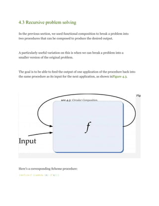
1. 4.3 Recursive problem solving
In the previous section, we used functional composition to break a problem into
two procedures that can be composed to produce the desired output.
A particularly useful variation on this is when we can break a problem into a
smaller version of the original problem.
The goal is to be able to feed the output of one application of the procedure back into
the same procedure as its input for the next application, as shown inFigure 4.3.
Fig
ure 4.3: Circular Composition.
Here’s a corresponding Scheme procedure:
(define f (lambda (n) (f n)))

2. Of course, this doesn’t work very well!1 Every application of f results in another
application of f to evaluate.
This never stops — no output is ever produced and the interpreter will keep
evaluating applications of f until it is stopped or runs out of memory.
We need a way to make progress and eventually stop, instead of going around in
circles. To make progress, each subsequent application should have a smallerinput.
Then, the applications stop when the input to the procedure is simple enough that
the output is already known.
The stopping condition is called thebase case, similarly to the grammar rules
in Section 2.4. In our grammar examples, the base case involved replacing the
nonterminal with nothing (e.g.,MoreDigits ::⇒⇒ ϵϵ) or with a terminal
(e.g., Noun ::⇒⇒ Alice). In recursive procedures, the base case will provide a solution
for some input for which the problem is so simple we already know the answer. When
the input is a number, this is often (but not necessarily) when the input is 0 or 1.
To define a recursive procedure, we use an if expression to test if the input matches
the base case input.
If it does, the consequent expression is the known answer for the base case. Otherwise,
the recursive case applies the procedure again but with a smaller input.

3. That application needs to make progress towards reaching the base case. This means,
the input has to change in a way that gets closer to the base case input.
If the base case is for 0, and the original input is a positive number, one way to get
closer to the base case input is to subtract 1 from the input value with each
recursive application.
This evaluation spiral is depicted in Figure 4.4. With each subsequent recursive call, the
input gets smaller, eventually reaching the base case.
For the base case application, a result is returned to the previous application. This
is passed back up the spiral to produce the final output.
Keeping track of where we are in a recursive evaluation is similar to keeping track of
the subnetworks in an RTN traversal.
The evaluator needs to keep track of where to return after each recursive evaluation
completes, similarly to how we needed to keep track of the stack of subnetworks to
know how to proceed in an RTN traversal.

4. Fig
ure 4.4: Recursive Composition.
Here is the corresponding procedure:
(define g (lambda (n)
(if (= n 0) 1
(g (- n 1)))))
Unlike the earlier circular f procedure, if we apply g to any non-negative integer it will
eventually produce an output. For example, consider evaluating (g 2).
When we evaluate the first application, the value of the parameter n is 2, so the predicate
expression (= n 0) evaluates to false and the value of the procedure body is the value of
the alternate expression, (g (- n 1)).
The subexpression, (- n 1) evaluates to 1, so the result is the result of applying g to 1.
As with the previous application, this leads to the application, (g (- n 1)), but this time
the value of n is 1, so (- n 1) evaluates to 0.
The next application leads to the application, (g 0). This time, the predicate expression
evaluates to true and we have reached the base case.
The consequent expression is just 1, so no further applications of g are performed and
this is the result of the application (g 0).

5. This is returned as the result of the (g 1) application in the previous recursive call, and
then as the output of the original (g 2) application.
We can think of the recursive evaluation as winding until the base case is reached,
and then unwinding the outputs back to the original application.
For this procedure, the output is not very interesting: no matter what positive
number we apply g to, the eventual result is 1.
To solve interesting problems with recursive procedures, we need to accumulate results
as the recursive applications wind or unwind.

6. This is returned as the result of the (g 1) application in the previous recursive call, and
then as the output of the original (g 2) application.
We can think of the recursive evaluation as winding until the base case is reached,
and then unwinding the outputs back to the original application.
For this procedure, the output is not very interesting: no matter what positive
number we apply g to, the eventual result is 1.
To solve interesting problems with recursive procedures, we need to accumulate results
as the recursive applications wind or unwind.