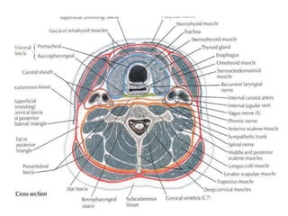
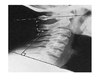
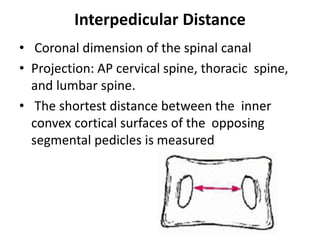
This document provides descriptions and guidelines for evaluating various radiographic lines and angles in the cervical, thoracic, and lumbar spine. It discusses anatomical structures like the retropharyngeal space and various methods for assessing spinal alignment, curvature, disc height, intervertebral angles, spinal canal dimensions, and detecting instability. Key measurements mentioned include Cobb's angle for scoliosis, Torg ratio for cervical stenosis, Ruth Jackson's lines for cervical flexion/extension stress, and Van Akkerveeken's measurement for lumbar instability. The document serves as a reference for radiologists and clinicians to evaluate common spinal radiographic findings.

1. Radiographic lines and angles
Dr. nishankverma
mpt – sports
Jamia MilliaIslamia

2. Retropharyngeal space

3. • It occupies the space posterior to the pharynx
and esophagus.
• Its anterior wall is made up of the bucco
pharyngeal fascia superiorly and the visceral
division of the middle fascia inferiorly
• The posterior wall is the alar layer of the deep
fascia
• The lateral boundary is the carotid sheath.
• This space extends from the base of the skull
to the level of the first and second thoracic
vertebra

7. Retropharyngeal abscess

8. Anterior vertebral line
Posterior vertebral line
Spinolaminar line
Posterior spinous line

9.  Assess four parallel lines.
• Anterior vertebral line (anterior margin of vertebral bodies)
• Posterior vertebral line (posterior margin of vertebral
bodies)
• Spinolaminar line (posterior margin of spinal canal)
• Posterior spinous line (tips of the spinous processes)
NOTE: These lines should follow a slightly lordotic curve,
smooth and without step-offs.
• Any malalignment should be considered evidence of
ligmentous injury or occult fracture cervical spine
immobilization should be maintained until a definitive
diagnosis is made.

12. Stress Lines of the Cervical Spine
Ruth Jackson’s lines
 Projection: Lateral cervical
spine (flexion, extension)
• Two lines are constructed on
each film
1) The first line is drawn along
the posterior surface of the axis
2) The second line is drawn
along the posterior surface of
the C7 body until it intersects
the axis
line

13. Normal Measurements
• Flexion - lines should intersect at the level of the
C5-C6 disc or facet joints.
• Extension - lines should intersect at the level of the
C4-C5 disc or facet joints.
• The intersection point represents the focus of
stress when the cervical spine is placed in the
respective positions
 The point of intersection does not appear to
correlate with the level of degenerative disc
disease
Muscle spasm, joint fixation, and disc degeneration
may alter the stress Point .

14. Cervical lordosis
• Depth method
Lateral cervical projection
• A line is drawn from the tip of the
odontoid process to the posterior
surface of C7
• A horizontal measure is taken
from the vertical line to the
posterior surface of the C4 body
(X)
• The average depth is 12 mm
• Negative – Kyphosis
• Largest values – Hyperlordosis
• The depth method provides a
more accurate assessment of
cervical lordosis

15. • Angle of curve
• Lateral cervical projection
• A line is drawn connecting the anterior and posterior
tubercles of the atlas
• Second line is drawn along the inferior endplate of C7
• Perpendicular lines are drawn from the atlas and C7
lines, and their angle of intersection is recorded as the
cervical lordosis (X°)
• The average value is 40 degrees
• Negative – kyphosis
• Large – hyperlordosis
 Note Less accurate than the depth method. Because
the measurements depend only on CI and C7

17. Torg ratio
• Cervical canal stenosis may cause a
neurological deficit, with neck stiffness as the
earliest symptom.
• Torg et al. have introduced a ratio called
the Torg ratio (spinal canal-vertebral body
ratio), that is not affected by magnification, and
is measured on lateral plain films of cervical
vertebrae.

18. • This measure is a ratio determined by the
distance from the center of the posterior
aspect of the vertebral bodies C3- C7 to the
spinal laminar line (the diameter of the spinal
canal) divided by the anteroposterior
diameter of the vertebral body anterior to the
canal.

20. • A ratio of ≥1.0 signifies absence of stenosis of
the spinal canal, but a ratio of ≤ 0.8 indicates
the presence of cervical spinal canal stenosis.
• Suk et al.from Korea determined the Torg ratio
of the cervical vertebrae (C3-C7) of 90 normal
Korean adults (without any abnormality of the
cervical vertebrae) and found mean ratios of
1.02 for females and 0.9 for males.
• In trauma patients in whom assessment of the
spinal canal is necessary for rapid detection of
cervical canal stenosis, the Torg ratio is used.

21. Lumbar spinal canal
Eisenstein's method
• Lateral lumbar projection
• Line is drawn connecting the tips of
the superior and inferior articular
processes of the same segment
• The canal width (x) is expressed as
the distance from the posterior body
margin to the middle portion of the
facet line
• The canal dimension should not fall
below 15 mm (although some use 14
mm or 12 mm as the cutoff)
• Smaller measurements may indicate
spinal stenosis
• Spinal stenosis is more accurately
assessed on axial MRI and CT
imagine.

22. Cobb’s Method of Scoliosis Evaluation
Cobb-Lippman method
Projection: AP spine.
End vertebrae
• Last segment that
contributes to the spinal
curvature.
• Extreme ends of the
scoliosis, where the
endplates tilt to the side
of the curvature concavity

23. • Endplate lines
• On the superior end vertebra, a line is drawn
through and parallel to the superior endplate
• On the inferior end vertebra, a line is
constructed in a similar manner through and
parallel to the inferior endplate
• This is the preferred method in scoliosis
assessment

24. • In patients with double scoliotic curves each
component should be measured.
• 5° progression of a scoliosis between two successive
radiographs is considered significant .
• Curvatures < 20° - No bracing or surgical intervention
• Patient between 10 and 15 years of age, careful
monitoring should be implemented to assess for
progression of 5° or more in any 3-month period.
• Curves between 20° and 40° - Bracing / Surgical
intervention
• Curvature progression in an immature spine, or
curvature in excess of 40° - Surgical intervention

25. Risser-Ferguson Method of Scoliosis
Evaluation
AP spine.
• Apical vertebra ------Most laterally placed
segment in the curve.
 Vertebral body center
• For each end vertebra and apical segment
diagonals are drawn from opposing corners of
the body to locate the body center
• Connecting line

26. • Two lines are constructed
connecting the body
centers of the apical
segment with each end
vertebra, and the
resultant angle is
measured
• This method gives values
approximately 25%
lower than those of
Cobb’s method (10°)
• Advocated its use for
larger curves

27. Interpedicular Distance
• Coronal dimension of the spinal canal
• Projection: AP cervical spine, thoracic spine,
and lumbar spine.
• The shortest distance between the inner
convex cortical surfaces of the opposing
segmental pedicles is measured

29. • This is a useful
measurement applied in
the evaluation of spinal
stenosis, congenital
malformation, and
intraspinal neoplasms
• The maximum
interpediculate distance
may be increased as a
result of pedicular
erosion from an
expanding spinal cord
tumor (Elseberg-Dyke
sign)

30. Thoracic Cage Dimension
• Straight back syndrome evaluation
• Projection: Lateral chest.
• The distance between the posterior sternum
and the anterior surface of the T8 body is
measured

32. Thoracic Kyphosis
• Lateral thoracic spine
• A line is drawn parallel to and
through the superior endplate of
the T1 body
• A similar line is drawn through
the inferior endplate of the T12
body.
• Perpendicular lines to these
endplate lines are then
constructed
• Intersecting angle is measured

33. Increased kyphosis
• Old age
• Osteoporosis
• Scheuermann’s disease
• Congenital anomalies
• Muscular paralysis
• Cystic fibrosis
Reduction in kyphosis
• straight back syndrome

34. Lumbar Intervertebral Disc Angles
• Lines are drawn
through and parallel to
each lumbar body
endplate
• The lines are extended
posteriorly until they
intersect
• Intersecting angle is
measured

36. Mean angle alteration
• Antalgia
• Muscular imbalance
• Improper posture
Facet syndrome -Increased Angle
Acute discal injuries -Decreased Angle

37. Lumbar Intervertebral Disc Height
• Lateral lumbar spine
• Visual assessment
• Disc height
compared with the
adjacent levels

38. Farfan’s method
• Anterior disc height (A) & posterior disc height
(P) are measured and expressed as a ratio to
disc diameter (D)
• These two ratios are then reduced to a ratio of
each other

40. • When segmental rotation is > 40° or lateral
flexion is > 20°, these methods become
unreliable.
 Decreased disc height
• Disc degeneration
• Post surgery
• Post chemonucleolysis
• Infection
• Congenital hypoplasia

41. Hadley’s S Curve
• Lumbar facet curve
 Projection: Oblique, AP lumbar spine
• Curvilinear line is constructed along
the inferior margin of the transverse
process and down along the inferior
articular process to the apophyseal
joint space
• Line is then continued across the
articulation to connect with the outer
edge of the opposing superior
articular process
• The resultant configuration of this
line will look like the letter S
• The key region of the S is the normally
smooth transition across the joint
space
• Abrupt interruption in the smooth
contour of this line may indicate facet
imbrication (subluxation)

43. Lumbar Gravity Line
The center of the L3 body is located by
intersecting diagonals from opposing body
corners
• A vertical line is constructed through center
point
• Relationship to the upper sacrum is assessed
• Center of gravity of the trunk passes through
the center of the L3 body and continues
vertically to intersect the sacral base

44. • Normally the vertical line will pass through the
anterior third of the sacral base.
• If this line passes anterior to the sacrum by > 0.5
inch (> 10 mm), an increase in shearing stresses
in an anterior direction between the lumbosacral
apophyseal joints may be occurring.
• Conversely, it has been suggested that a
posterior shift in this gravity line may indicate
increased weight bearing forces on these same
lumbosacral joints that may also be active in the
production of low back pain

46. Van Akkerveeken’s Measurement of
Lumbar Instability
• Projection: Lateral lumbar
spine (neutral, flexion,
extension).
• Two lines are drawn
through and parallel to
opposing segmental
endplates until they
intersect posteriorly.
• The distance from the
posterior body margins to
the point of intersection is
then measured.

47. Normal Measurements
• There should be < 1.5 mm displacement, as
determined by either measurement method
• If there is > 1.5 mm (3mm) difference in
measurement, then it is likely that nuclear,
annular, and posterior ligament damage at the
displaced segment is present

48. Lumbar Lordosis
• Lumbar curve, lumbar spinal angle,
lumbar angle Projection: Lateral
lumbar spine.
• Line is drawn through and parallel
to the superior endplate of the
first lumbar segment
• Second line is drawn through the
superior endplate of the first sacral
segment
• Perpendiculars are then created,
and the angle at their intersection
is measured
• A wide variation exists within
normal individuals.
• The average appears to be 50-60°

49. Meyerding’s Grading Method in
Spondylolisthesis
• The superior surface of the first
sacral segment is divided into four
equal divisions. The relative
position of the posterior inferior
corner of the L5 body to these
segments is then made
• The posterior inferior corner of the
L5 body should be aligned with the
posterior-superior corner of the
first sacral segment.
• The same assessment can be
applied to other spinal levels by
dividing the superior endplate of
the segment below the
spondylolisthesis into four equal
spaces.

50. • In spondylolisthesis, > 12° dynamic angulation
or 8% translation on flexion-extension views is
considered evidence of instability
• The degree of anterolisthesis of the affected
vertebral body can be categorized according
to the division in which the posterior-inferior
corner of the body lies

51. • Grade I – Less than 25 percent slip
• Grade II – Between 25 and 50 percent slip
• Grade III – Between 50 and 75 percent slip
• Grade IV – More than 75 percent slip
• Grade V – This means that the upper vertebral
body has slide all the way forward off the
front of the lower vertebral body. This is a
special situation that is called
a spondyloptosis and is very rare.

52. Lumbosacral Angle
• Two lines
• First, a horizontal line is
made parallel to the
bottom edge of the film
• Second, an oblique line is
drawn through and parallel
to the sacral base.

54. Sacral angle / Barge's angle
• The angle of the
superior margin of
the sacrum from the
horizontal plane,
measured in the
sagittal plane
• lumbar lordosis
increased if the sacral
angle increased

55. Ullmann’s Line
• Garland-Thomas line, right-angle
test line
• Projection: Lateral lumbar spine,
lumbosacral
• Parallel to and through the sacral
base
• Perpendicular to the first line at
the anterior margin of the sacral
base.
• The relationship of the L5 body
to this perpendicular line is then
assessed
• Anterior margin of the L5 body
crosses the perpendicular line,

56. • Anterolisthesis
• This is a useful line for detecting the presence
of spondylolisthesis when there is poor
visualization of the pars region.

57. Scotty dog sign
• The scotty dog sign refers to the
normal appearance of the lumbar
spine when seen on oblique
radiographic projection.
• On oblique views, the posterior
elements of vertebra form the figure
of a Scotty dog with:
• the transverse process being the nose
• the pedicle forming the eye
• the inferior articular facet being the
front leg
• the superior articular
facet representing the ear
• the pars interarticularis (the portion
of the lamina that lies between the
facets) equivalent to the neck of the
dog.

58. • If spondylolysis is
present, the pars
interarticularis, or the
neck of the dog, will
have a defect or break.
It often looks as if the
dog has a collar around
the neck (or
decapitation for those
with a bloodier
imagination).

59. Slip angle
• as slip progresses, area of contact between L5 & S1 decreases &
body of L5 tilts forward on sacrum;
- this is referred to as sagittal rotation, angle of slipping, roll,
L5/S1 kyphosis, or gibbu
• slippage is not present in pts who have mild (grade-I or II)
spondylolisthesis, but is more common in pts who have a 50 %
slip & always present in pts w/ 75 % slip
• Measurement
The slip angle (A) is a measure of kyphosis at the listhetic level.
• It is calculated by determining the angle between a line
perpendicular to the posterior margin of the subjacent vertebral
body and a line parallel to the superior end plate of the olisthetic
vertebra.

61. Upper extremity

62. Upper Extremity Measurements
• Acromioclavicular joint space
• AP or postero anterior (PA) shoulder.
• The joint space is measured at the superior
(S) and inferior (I) borders, and the two values
are averaged.

64. Decreased joint space
• Degenerative joint disease
Increased joint space
• Traumatic separation
• Hyperparathyroidism
• Rheumatoid arthritis

65. Acromiohumeral joint space
• AP shoulder.
• The distance between the inferior surface of
the acromion and the articular cortex of the
humeral head is measured.

67. Narrowed space (<7mm)
• Superior shoulder displacement, which is
often secondary to shoulder impingement
syndrome with rotator cuff tendonopathy.
Enlarged space (>11mm)
• Dislocation
• Joint effusion
• Paralysis
• Brachial plexus lesions (drooping shoulder)

68. Glenohumeral joint space
• AP shoulder with external rotation.
• The measurements are made at the superior,
middle, and inferior aspects of the joint.
• These are combined and averaged.
• Each distance is ascertained between the
opposing articular surfaces
• The average joint space is 4-5 mm

70. Joint space diminished
• Degenerative arthritis,
• Calcium pyrophosphate dihydrate (CPPD)
crystal disease
• Post-traumatic arthritis.
Widened space
• Acromegaly
• Posterior humeral dislocation.

71. Axial Relationships of the Shoulder
Humeral axial angle
• AP shoulder with external rotation.
• Humeral shaft line (A). A line is drawn
through and parallel to the humeral shaft.
• From apex of greater tuberosity a line is drawn
towards the medial surface
• The average humeral angles are 60° for males
and 62° for females
• This relationship may be altered following a
fracture, especially in the surgical neck.

73. Elbow - Anterior humeral line
• On the lateral elbow projection a line drawn
along the anterior surface of the humerus
should intersect the middle third of the lateral
condylar ossific center.
• If the line passes anterior or posterior to the
middle third of the lateral condyle, a fracture
may be present

75. Radiocapitellar Line
• Lateral elbow.
• A line is drawn through the
center of and parallel to the
long axis of the radius and
is extended through the
elbow joint.
• This line should pass
through the center of the
capitellum in all stages of
flexion of the elbow
• This assists in determining
the presence of radial head
subluxation (pulled elbow)
or dislocation

76. Hand - Capitolunate sign
• On the lateral wrist
projection, lines are
drawn to approximate the
long axes of the lunate
and capitate.
• Assessment assists in
determining the presence
of fracture or dislocation.

77. Scapholunate angle (scaphoid tilt)
• On the lateral wrist
projection, lines are
drawn to approximate
the long axes of the
scaphoid and lunate.
• If the angle is greater
than 80 and the lunate is
also extended
(dorsiflexed), dorsal
intercalated segmental
instability (DISI) is
suggested.

78. Metacarpal Sign
• PA hand
• A line is drawn tangentially through the articular
cortex of the fourth and fifth metacarpal heads
• The line should pass distal to or just touch the
third metacarpal head
• Postive in
• Turner’s syndrome
• Fracture deformity
• Pseudo/ pseudo-pseudo
• hypoparathyroidism

80. Metacarpal index
• Determined by
dividing the length of
each of the last four
metacarpals by the
width of its midpoint
and averaging the
values
• Marfans patients are
often greater than 8.4,
while normal are less
than 8.

81. Radiolunate angle (lunate tilt)
• On the lateral wrist
projection, lines drawn to
approximate the long axes
of the radius and lunate
should be parallel.
• If the lunate is flexed more
than 15 degrees, volar
intercalated segment
instability (VISI) is
suggested

82. • If the angle is greater than 10 degrees in
extension, dorsal intercalated segment
instability (DISI) is suggested.
• Occasionally VISI and usually DISI occur with
scapholunate dissociation
• VISI is also related to triquetrolunate
dissociation

83. Radioulnar variance
• On the antero posterior wrist projection, the distal
ulnar articular surface should align with the inner
portion of the distal radial articular surface.
• Short ulna
• Avascular necrosis of the lunate (Kienbock's disease)
• Greater carpal stress distribution to the radius
• Long ulna
• Greater carpal stress distribution to the ulna.
• Differences of less than 5 mm are probably not
significant.

84. Lower extremity

85. Teardrop Distance
• Medial joint space of hip.
• The distance between the most medial
margin of the femoral head and the outer
cortex of the pelvic teardrop is measured
 ABNORMAL MEASUREMENT
• >11 mm or
• > 2 mm discrepancy from right to left
(Waldenstrom’s sign)
• Left to right discrepancies of > 1 mm will
be present in 90% of hip joint effusions.
• Legg-Calve-Perthes disease
• Septic arthritis
• Other inflammatory diseases

87. Hip Joint Space Width
• Three measurements are made of the joint cavity
• Superior joint space: Space between the most
superior point on the convex articular surface of
the femur and adjacent acetabular cortex.
• Axial joint space: Space between the femoral
head and acetabulum immediately lateral to the
acetabular notch.
• Medial joint space (teardrop distance): Space
between the most medial surface of the femoral
head and opposing acetabular surface

88. • The superior and axial compartments are
approximately equal (4 mm), The medial
space is twice the distance (8 mm)
 Superior joint space Reduction
• Degenerative joint disease
 Axial joint space
• Degenerative arthritis
• Inflammatory arthritis
 Medial joint space
• Degenerative or inflammatory arthritis

90. Acetabular Depth
• A line is drawn from the superior margin of
the pubis at the symphysis joint to the upper
outer acetabular margin
• The greatest distance
from this line to the
acetabular floor is
measured

91. • An acetabular depth < 9 mm in females and <
7 mm in males is considered to be shallow and
dysplastic, which may be a factor in
precipitating degenerative joint disease of the
hip.

92. Acetabular center-edge angle
• A vertical line is drawn
through the center point of
the femoral head.
• Another line is constructed
through the femoral head
center to the outer upper
acetabular margin.
• The angle formed is then
measured.

93. • Shallow angle
• Acetabular dysplasia
• degenerative joint disease.
• It provides a measure of coverage of the
femoral head, which means the amount of the
acetabulum primarily concerned with weight
bearing

94. Symphysis Pubis Width
• The measured distance
is between the
opposing articular
surfaces, halfway
between the superior
and inferior margins of
the joint

95. • Widening of the symphysis
• cleidocranial dysplasia,
• bladder exostrophy

96. Acetabular index

97. • Horizontal line is drawn through the right and left tri
radiate cartilage (Hilgenreiner's Line).
• Another line is drawn along each of the acetabuli to
intersect the horizontal tri radiate cartilage line
• Dividing the hip into 4 quadrants.
• The proximal medial femur should be in the lower
medial quadrant, or the ossific nucleus of the femoral
head, if present (usually observed in patients aged 4-7
month), should be in the lower medial quadrant.
• The acetabular index is the angle between the
Hilgenreiner line and a line drawn from the tri radiate
epiphysis to the lateral edge of the acetabulum

99. • The angles of intersection (x°) should not exceed standards based
on age:
• at Birth < 36 degrees in females,
• < 30 degrees in males;
• 6 months < 28 degrees in females,
• < 25 degrees in males;
• 1 year < 25 degrees in females,
• 24 degrees in males;
• 7 years < 19 degrees in females,
• < 18 degrees in males
• Enlarged angle
• Acetabular dysplasia
• Congenital dislocation of the hip
• Shallow angle - Down syndrome

100. Iliac Angle and Index

101. • A line is drawn through the triradiate cartilage
at the pelvic brim
• A second line is constructed tangential to the
most lateral margin of the iliac wing and iliac
body
• Iliac index: This is the sum of both the iliac
angles and the acetabular angles divided by 2.

102. • The iliac index is most useful in the
determination of Downs syndrome.
• When the index is < 60, Down¡¦s syndrome is
probable; when the index is 60-68, the
syndrome is possible; if > 68, the syndrome is
unlikely

103. Iliofemoral Line
• A curvilinear line is constructed along the outer
surface of the ilium, across the joint, and onto the
femoral neck
• A small portion of the superior femoral head
may cause a slight convexity in the line.
• The most important normal feature is that the
line should be bilaterally symmetrical.
• A discrepancy in symmetry may be the result of
congenital dysplasia, slipped femoral capital
epiphysis, dislocation, or fracture

105. Femoral Angle
• Femoral angle of
incidence, femoral neck
angle, Mikulicz’s angle.
• Two lines are drawn
through and parallel to
the midaxis of the
femoral shaft and
femoral neck.
• The angle subtended is
then measured

107. Skinner’s Line
• A line is drawn through and parallel to the axis of the
femoral shaft.
• A second line is constructed at right angles to the shaft
line and tangential to the tip of the greater trochanter.
• The relationship of the fovea capitis to this trochanteric
line is assessed.
• The fovea capitis should lie above or at the level of the
trochanteric line.
• The fovea lies below this line when there is a superior
displacement of the femur relative to the femoral head.
• The most common causes are fracture and conditions
leading to coxa vara

109. Klein’s Line
• A line is constructed tangential
to the outer margin of the
femoral neck.
• The degree of overlap of the
femoral head will be apparent.
• Comparison should be made
with the opposite side
• Generally there will be the
same degree of overlap of the
femoral head

110. • In most normal hips the outer margin of the
femoral head will be lateral to the line.
• This line can be drawn on both the AP and
frog-leg projections
• If the femoral head does not overlap the line
or if there is asymmetry from side to side,
then slippage of the femoral capital epiphysis
should be suspected.

111. Axial Relationships of the Knee
• AP knee.
• Four lines and two angles are
drawn
• Femoral shaft line (A). A line is
drawn through and parallel to the
midaxis of the femoral shaft.
• Tibial shaft line (B). A line is drawn
through and parallel to the midaxis
of the tibial shaft.
• Femoral condyle line (C). A line is
drawn through and tangential to
the articular surfaces of the
condyles

112. • Tibial plateau line (D). A line is drawn through the
medial and lateral tibial plateau margins
• Femoral angle (FA). This is the angle formed
between the femoral shaft and femoral condyle
lines.
• Tibial angle (TA). This is the angle formed
between the tibial shaft and tibial plateau lines
Significance.
• These angles will be altered in fractures and
other deformities about the knee.

114. Patellar Position
• Patella alta evaluation
• Lateral knee (semiflexed)
• Patellar length (PL). This is the
greatest diagonal dimension
between the superior and the
inferior poles.
• Patellar tendon length (PT).
The distance measured is
between the insertion points
of the posterior tendon
surface at the inferior patellar
pole and the notch at the
tibial tubercle.

115. • Normal Measurements.
• Patellar length and patellar tendon length are usually
equal to each other.
• A normal variation up to 20%
• > 20% - patella alta
• chondromalacia patellae.
• A low-riding patella (patella baja)
• Polio
• Achondroplasia
• juvenile rheumatoid arthritis
• tibial tubercle transposition

116. Patellar Malalignment
• Patellar tracking, patellar
subluxation,
patellofemoral joint
incongruence.
• Tangential knee (skyline)
• Patella apex The patella is
centered when its apex is
directly above the
deepest section of the
intercondylar sulcus

117. • Sulcus angle by drawing lines from the highest
points on the medial and lateral condyles to
the lowest point of the intercondylar sulcus,
an angle is formed.
• Normally, this should be 138° ± 6°. Larger
angles (shallow intercondylar groove)
predispose the individual to subluxation and
dislocation.

118. Axial Relationships of the Ankle
• Four lines and two
angles are constructed.
• Tibial shaft line (A). A
line is drawn through
and parallel to the tibial
shaft.
• Medial malleolus line
(B). A line is drawn
tangential to the
articular surface of the
medial malleolus.

119. • Lateral malleolus line (C). A line is drawn
tangential to the articular surface of the
lateral malleolus.
• Talus line (D). A line is drawn tangential to the
articular surface of the talar dome.

120. • Tibial angle (I). The angle is formed medially
between the medial malleolus line and talus
line.
• Fibular angle (II). The angle is formed laterally
between the lateral malleolus line and talus
line

121. • Significance.
• These angles will be altered in fractures of the
malleoli, ankle mortise instability, and
tibiotalar slant deformities.
• The tibiotalar joint space is measured at the
lateral and medial joint margins.

122. Boehler’s Angle
• Axial relationships of the
calcaneus, tuber angle.
• Lateral foot, lateral calcaneus.
• The three highest points on the
superior surface of the calcaneus
are connected with two tangential
lines
• The angle formed posteriorly is
then assessed
• Normal Measurements.
• The angle formed posteriorly
averages between 30° and 35° in
most normal subjects but may
range between 28° and 40°.

123. • Any angle < 28° is abnormal.
• The most common cause for an angle < 28° is
a fracture with displacement through the
calcaneus.
• Dysplastic development of the calcaneus
may also disturb the angle.

124. First metatarsal angle
• On the antero posterior
foot projection, lines drawn
to approximate the long
axes of the first metatarsal
and proximal first phalanx
should form an angle (x°) of
less than 15 degrees.
• An increased angle
indicates a hallux valgus
deformity.

125. Meary's angle
• On the lateral foot projection, lines drawn
to approximate the longitudinal axis of
the first metatarsal and talus should be
parallel
• If the lines are not parallel and form an
angle that is greater than 0 degrees,
forefoot cavus deformity is indicated.

127. Calcaneal pitch
• A line is drawn from the plantar most surface
of the calcaneus to the inferior border of the
distal articular surface.
• The angle made between this line and the
transverse plane (or the line from the plantar
surface of the calcaneus to the inferior surface
of the 5th metatarsal head) is the calcaneal
pitch

130. • A decreased calcaneal pitch is consistent with
pes planus.
• Unfortunately, there have been differing
opinions between authors concerning the
normal range of calcaneal pitch 18 to
• 20°is generally considered normal (12),
although measurements ranging from 17 to
32°