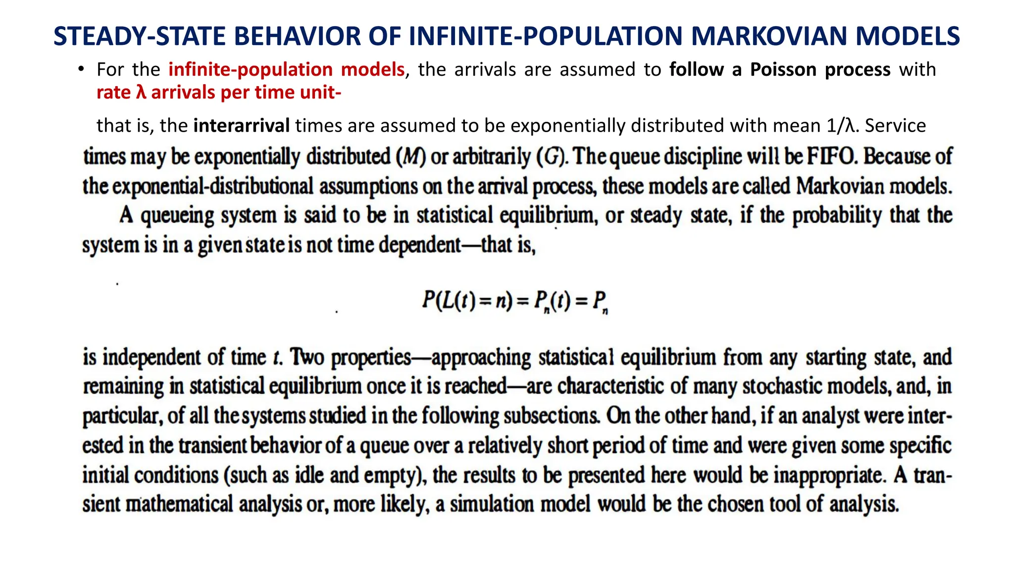
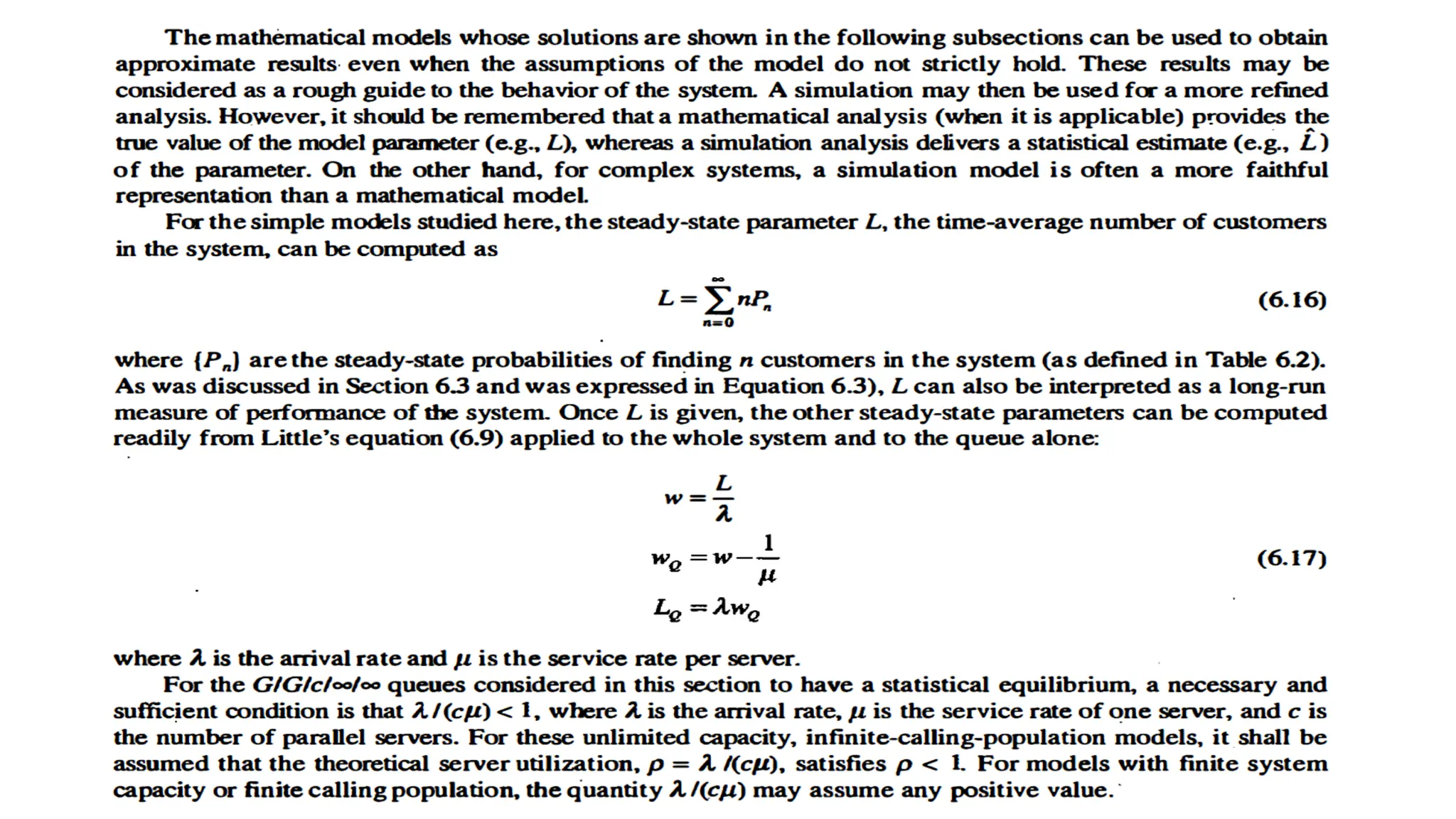
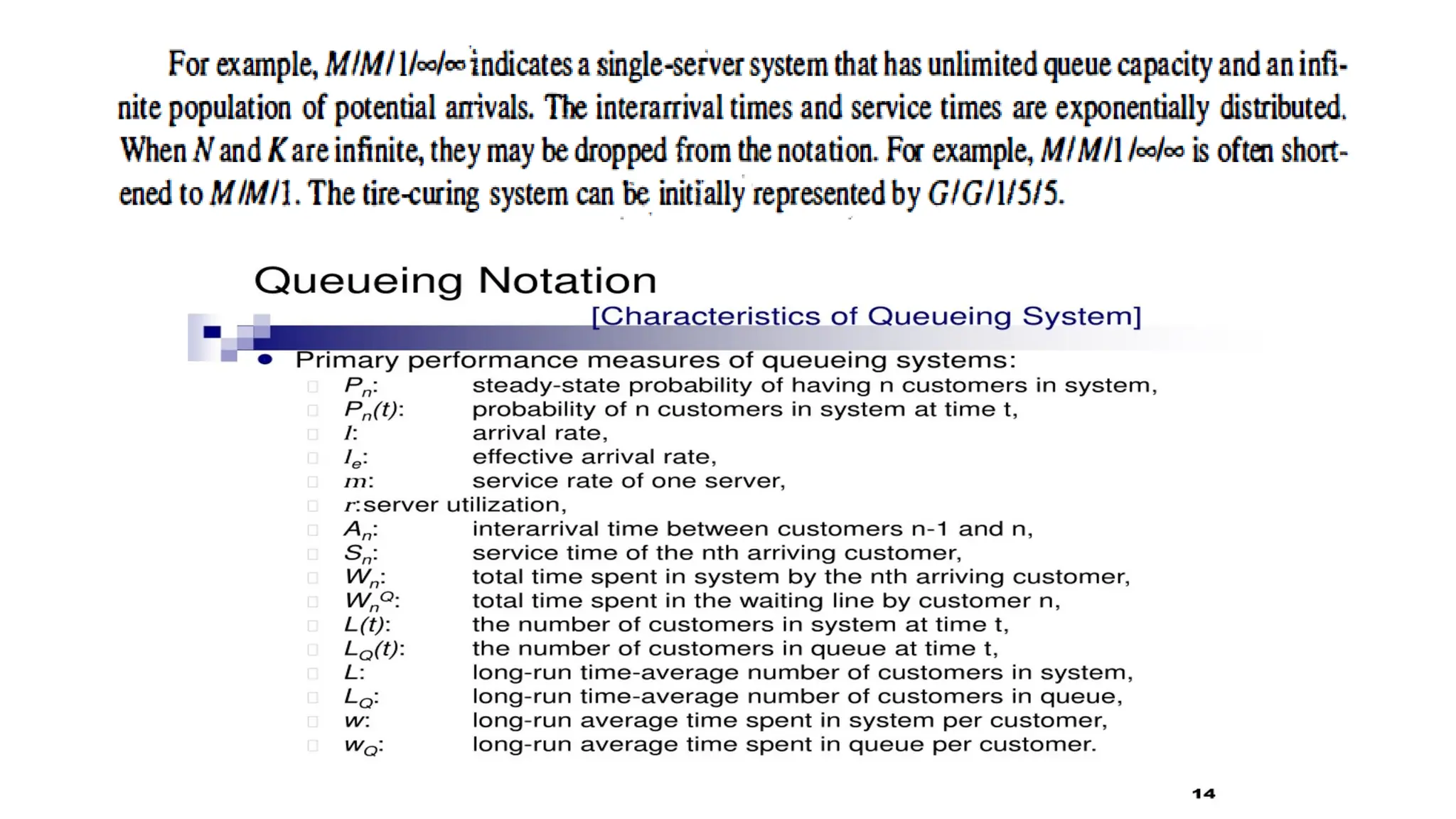
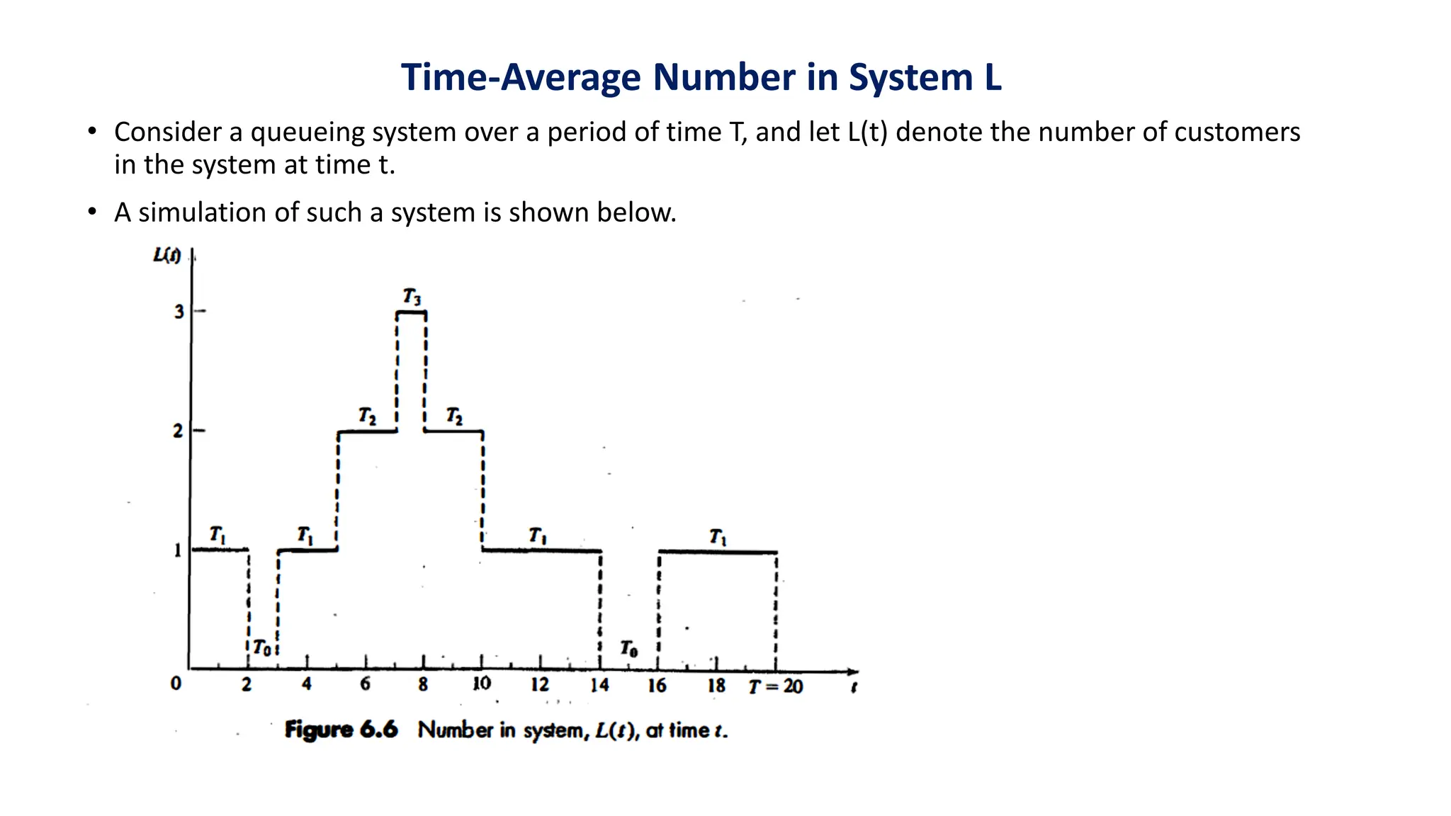
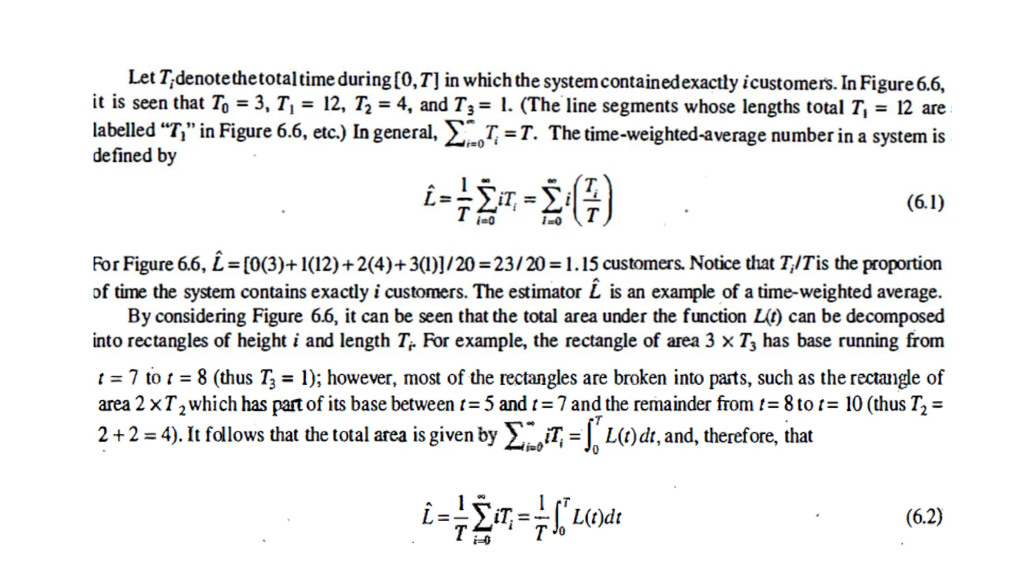
9. • The service times of successive arrivals are denoted by S1, S2, S3, . . . They may be constant or of random
duration.
• In the latter case, {S1, S2, S3, . . . } is usually characterized as a sequence of independent and identically
distributed random variables.
• The exponential, Weibull, gamma, lognormal and truncated normal distributions have all been used
successfully as models of service times in different situations.
• Sometimes services are identically distributed for all customers of a given type or class or priority,
whereas customers of different types might have completely different service-time distributions.
• In addition, in some systems, service times depend upon the time of day or upon the length of the
waiting line.
• For example, servers might work faster than usual when the waiting line is long, thus effectively reducing
the service times.
• A queueing system consists of a number of service centers and interconnecting queues.
• Each service center consists of some number of servers, c, working in parallel;
that is, upon getting to the head of the line, a customer takes, the first available server.
• Parallel service mechanisms are either single server (c = 1), multiple server (1 < c < ∞ ), or unlimited
servers (c = ∞ ).
• A self-service facility is usually characterized as having an unlimited number of servers.
Service Times and Service Mechanism
14. Long Run Measures of Performance of Queuing Systems
• The primary long-run measures of performance of queueing systems are the long-run time-
average number of customers in the system (L) and in the queue (LQ), the long-run average time
spent in system (w) and in the queue (wQ) per customer, and the server utilization, or
proportion of time that a server is busy (p).
• The term "system" usually refers to the waiting line plus the service mechanism, but, in general,
can refer to any subsystem of the queueing system; whereas the term "queue" refers to the
waiting line alone.
• Other measures of performance of interest include the long-run proportion of customers who
are delayed in queue longer than to time units, the long-run proportion of customers turned
away because of capacity constraints, and the long-run proportion of time the waiting line
contains more than k0 customers.
15. Time-Average Number in System L
• Consider a queueing system over a period of time T, and let L(t) denote the number of customers
in the system at time t.
• A simulation of such a system is shown below.
16.
17.
18.
19.
20. Average Time Spent in System Per Customer w
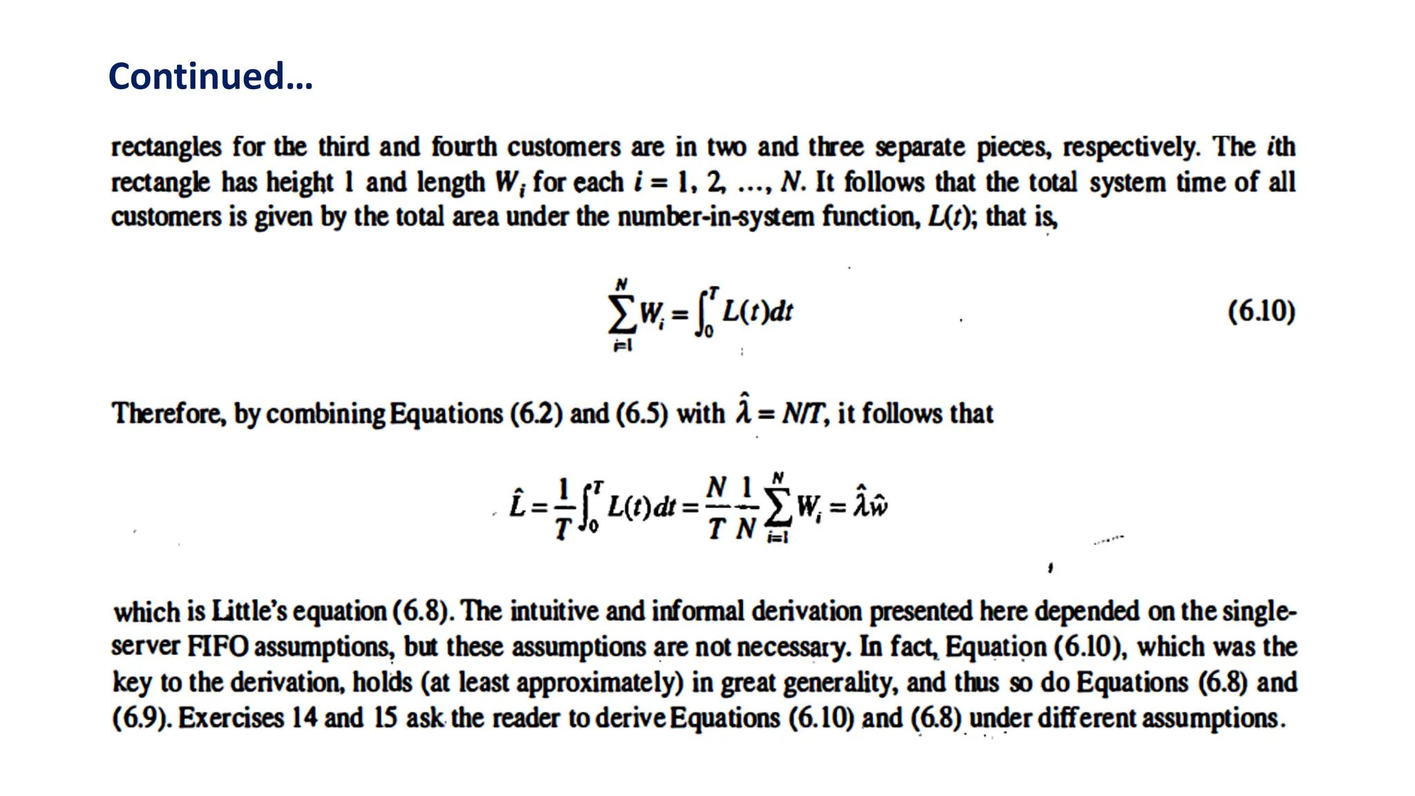
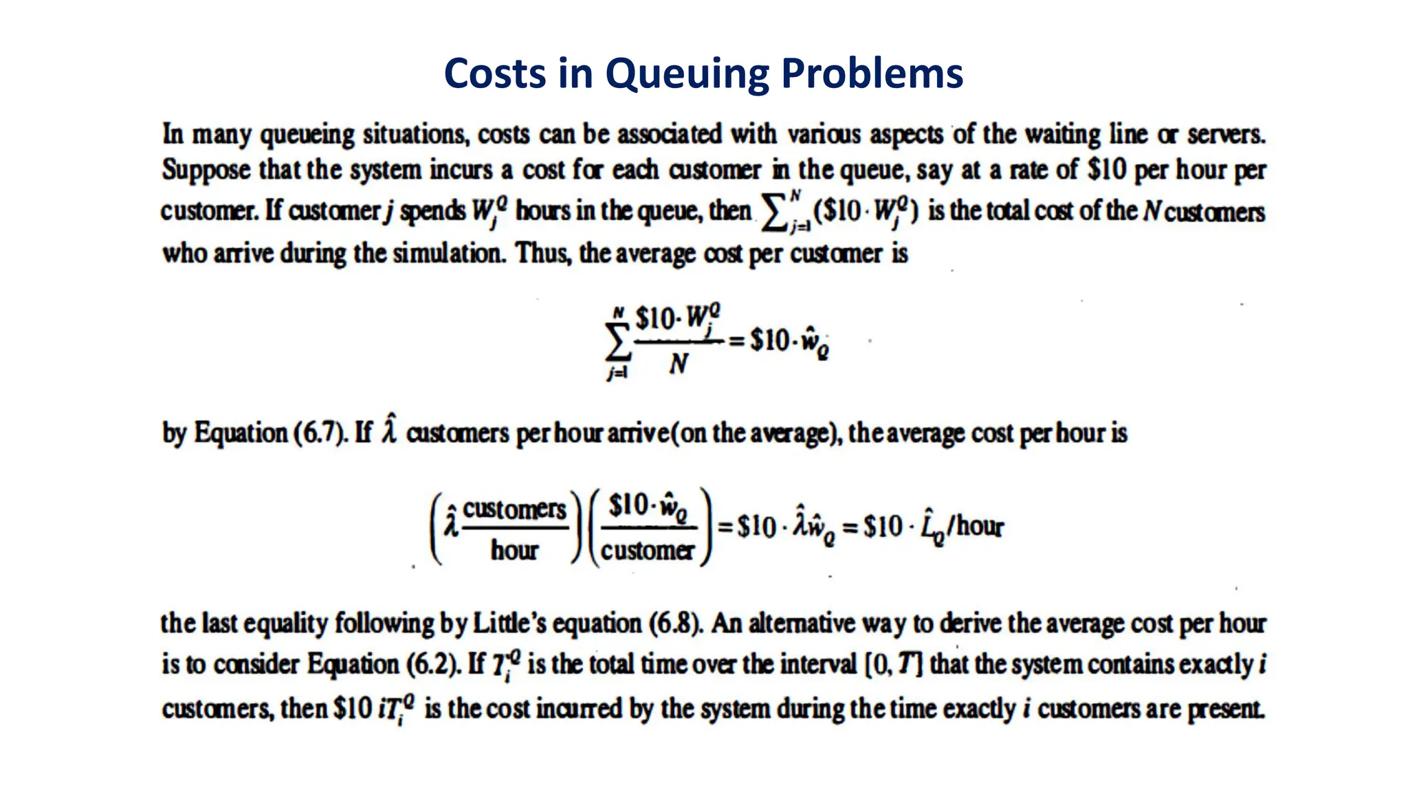
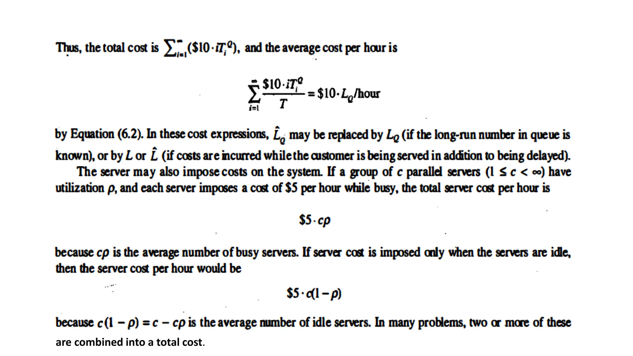
• If we simulate a queueing system for some period of time, say T, then we can record the time
each customer spends in the system during [0, T], say W1, W2, . . ., WN> where N is the number
of arrivals during [0, T].
• The average time spent in system per customer, called the average system time, is given by the
ordinary sample average,
27. Server Utilization in G/G/1/∞/∞ Queues
• Consider any single-server queueing system with average arrival rate λ customers per time unit,
Average service time E(S) = 1/µ time units, and infinite queue capacity and calling population
Notice that E(S) = 1/µ implies that,
when busy, the server is working at the rate µ customers per time unit, on the average µ is
called the service rate.
• The server alone is a subsystem that can be considered as a queueing system in itself; hence, the
conservation Equation, L = λw, can be applied to the server.
• For stable systems; the average arrival rate to the server, say λ must be identical to the average
arrival rate to the system, λ (certainly λs ≤ λ customers cannot be served faster than they arrive-
but, if λs < λ, then the waiting line would tend to grow in length at an average rate of
28.
29.
30.
31. Server Utilization in G/G/c/∞/∞ Queues
• Consider a queueing system with c identical servers in parallel.
• If an arriving customer finds more than one server idle, the customer chooses a server without
favouring any particular server. (For example, the choice of server might be made at random.)
• Arrivals occur at rate λ from an infinite calling population, and each server works at rate
µcustomers per time unit.
• From Equation (6.9), L = λw, applied to the server subsystem alone, an argument similar to the
one given for a single server leads to the result that, for systems in statistical equilibrium, the
average number of busy servers, say L,, is given by,
32.
33.
34. Server Utilization and System Performance
• System performance can vary widely for a given value of utilization ρ.
• Consider a G/G/1/∞/∞ queue, that is, a single server queue with arrival rate λ, server rate µ and
utilization,
40. STEADY-STATE BEHAVIOR OF INFINITE-POPULATION MARKOVIAN MODELS
• For the infinite-population models, the arrivals are assumed to follow a Poisson process with
rate λ arrivals per time unit-
that is, the interarrival times are assumed to be exponentially distributed with mean 1/λ. Service