This document is a doctoral thesis submitted by Dimitrios Bisias to MIT's Sloan School of Management. The thesis contains four essays on applications of optimal portfolio theory. The first essay studies optimal trading of arbitrage opportunities under value-at-risk and collateral constraints. The second essay extends this to consider the impact of model misspecification. The third essay applies portfolio theory to analyze biomedical funding allocation at the National Institutes of Health. The fourth essay investigates how risk constraints and model misspecification affect market statistics. The thesis was certified by Andrew Lo and accepted in partial fulfillment of the requirements for a PhD in Operations Research.


![Chapter 1
Optimal trading of arbitrage
opportunities under constraints
In financial economics, an arbitrage is an investment opportunity that is too good
to be true when there are no market frictions. In actual financial markets however,
there are frictions and even if there are arbitrage opportunities the investors may not
be able to fully exploit them due to the constraints they face.
We will explore two kinds of risky arbitrage opportunities when there are market
frictions. The first one is a case of a textbook arbitrage, a convergence trade strategy.
The second is a case of a statistical arbitrage, a mean reversion trading strategy. These
two strategies are two of the most popular trading strategies that hedge funds follow,
so studying them in detail when there are market frictions is a valuable exercise.
A convergence trade is a trading strategy consisting of long/short positions in two
similar assets, where we buy the cheap asset, we short the expensive asset and we wait
until the prices of the two assets to converge which we know it will happen for sure
some particular time in the future. An example of this trade involves the difference
in price between the on-the-run and the most recent off-the-run security. An on-
the-run security is the most recently issued, and hence most liquid, of a periodically
issued security. Since an on-the-run security is more liquid it trades at a premium
to off-the-run securities [29]. A convergence trade involves taking a long position in
the most recent off-the-run security and shorting the on-the-run security. The on-
29](https://image.slidesharecdn.com/938838223-mit-230323123641-6cde2771/85/938838223-MIT-pdf-29-320.jpg)
![the-run will become off-the-run upon the issue of a newer security and then there
will be almost no difference between the two securities in our trade so their prices
will converge. Another example involves investing in Treasury STRIPS with identical
maturity dates but different prices.
A mean reversion trading strategy involves investing in an asset or a portfolio of
assets whose value is a mean reverting process. Since most price series in the equity
space follow random walk, this strategy most commonly involves investing in a port-
folio of non-mean-reverting assets whose value is a stationary mean reverting series.
These price series that can be combined in such a way are called cointegrating. A
classic statistical arbitrage example is the pairs trading, which is the first type of
algorithmic mean reversion trading strategy invented by institutional traders, report-
edly by the trading desk of Nunzio Tartaglia at Morgan Stanley [64]. The statistical
arbitrage pairs trading strategy bets on the convergence of the prices of two similar
assets whose prices have diverged without a fundamental reason for this.
These arbitrage opportunities are risky under market frictions. In particular the
first case is exposed to the “divergence risk”, i.e. the fact that the pricing differential
between the two similar assets can diverge arbitrarily far from 0 prior to its conver-
gence at some particular time in the future. The second case is exposed both to the
“divergence risk” and to the “horizon risk”, in other words the fact that the times at
which the spread will converge to its long run mean are uncertain.
We will explore the optimal portfolio allocation of a risk averse investor who
invests in N convergence trades or mean reverting trading strategies, while facing
constraints. In particular, we will study the optimal trading strategy when he faces
VaR constraints or collateral constraints. Risk sensitive regulation, such as the VaR
constraint, has lately become a central component of international financial regu-
lations. Collateral or margin constraints, where the investor has to have sufficient
wealth to secure the liabilities taken by short positions, have been ubiquitous in the
financial transactions for centuries and margin calls have been behind several crises
including the LTCM debacle[54].
In the rest of this chapter, we will discuss the relevant literature review. Then we
30](https://image.slidesharecdn.com/938838223-mit-230323123641-6cde2771/85/938838223-MIT-pdf-30-320.jpg)
![will discuss about the setup of the model and the constraints, we will find the optimal
trading strategy of the investor and finally we will explore the characteristics of this
optimal strategy.
1.1 Literature review
Merton studied the problem of optimal portfolio allocation in a continuous time set-
ting without any market frictions [59]. The optimal portfolio involves two terms: a
market timing term and a hedging demand term. The first term is a myopic term that
represents the optimal allocation if you were interested at each time instant t only for
an horizon dt ahead. The second term represents the investor’s additional demand
due to the covariance of the wealth process with the attractiveness of the available
investment opportunities. Although Merton gives an analytical general solution this
is expressed in terms of the partial derivatives of the value function and additional
work is needed to derive the solution in terms of the model parameters. Additionally
it assumes that there are no market frictions.
Optimal trading of mean reversion trading strategies have been studied by both
Boguslavsky and Boguslavskaya [15] and Jurek and Yang [48]. They have found
analytical solutions for the optimal weight of a single mean reverting trading strategy
for risk averse CRRA investors. Their analysis is similar with the one in Kim and
Omberg [49], where they assume that there is a risk free asset with a constant risk-
free rate and a single risky asset with a mean reverting risk premium, which implies
a mean reverting instantaneous Sharpe ratio. In all the cases they have assumed that
there are no market frictions whatsoever.
Longstaff and Liu [53] have studied the problem of optimal trading of a single
convergence trade under a margin constraint. For the single convergence trade case
both VaR constraints and margin constraints collapse in the same constraint and the
problem is significantly easier. In addition by studying only convergence trades they
have taken out one important dimension of risk, the horizon risk, keeping only the
divergence risk. Brennan and Schwarz [17] have also studied the problem of optimal
31](https://image.slidesharecdn.com/938838223-mit-230323123641-6cde2771/85/938838223-MIT-pdf-31-320.jpg)
![trading of a single convergence trade including transaction costs when the arbitrage
potential is restricted by position limits.
The literature is rich with papers that study the existence of an equilibrium where
there exists mispricings. This persistence of mispricings is typically attributed to
agency problems, frictions or some kind of risk. Unlike textbook arbitrages, which
generate riskless profits and require no capital commitments, exploiting real-world
mispricings requires the assumption of some kind of risk. Shleifer and Vishny [74]
emphasized that risks such as the uncertainty about when the pricing differential
will converge to 0 and the possibility of a divergence of the mispricing prior to its
elimination may play a role in limiting the size of positions that arbitrageurs are
willing to take, contributing to the persistence of the arbitrage in equilibrium. Basak
and Choitoru [6] also showed that arbitrage can persist in equilibrium when there are
frictions. They study dynamic models with log utility and heterogeneous beliefs in
the presence of margin requirements and other portfolio constraints.
With respect to the constraints, Basak and Shapiro [7] study the problem of opti-
mal trading strategy of a risk averse investor who faces finite horizon VaR constraints
in a complete markets setting using the martingale representation approach [4]. Here
again there are no constraints in the optimal portfolio allocation at each time t but
there is only one constraint in the wealth at some finite horizon. Finally, Geanakoplos
[33] studies the collateral constraints, how these determine an equilibrium leverage
and how this leverage changes over time, the so-called leverage cycles.
Let us now discuss about the setup of the model and the constraints and find the
optimal trading strategy of the investor.
1.2 Analysis
We assume we have a risk averse investor maximizing the expected continuously
compounded rate of return or equivalently the expected logarithm of his final wealth
E(lnWT ). There are two cases to consider. In the first case, the investor can invest
in a risk-free asset and N non-redundant convergence trades, modeled as correlated
32](https://image.slidesharecdn.com/938838223-mit-230323123641-6cde2771/85/938838223-MIT-pdf-32-320.jpg)

![In our case we have N of these mean reverting processes and we assume that they
are modeled as a multivariate Ornstein-Uhlenbeck process, which is defined by the
following stochastic differential equation:
dSt = −Φ(St − S̄)dt + σdZt (1.2)
Above Φ is a N-by-N square transition matrix that characterizes the deterministic
portion of the evolution of the process, S̄ is the vector representing the unconditional
mean of the process, σ is a N-by-K matrix that drives the dispersion of the process
and Zt is a Brownian motion in RK
.
The Ornstein-Uhlenbeck process has the nice property that its conditional distri-
bution is normal at all times, with mean equal to
Et[St+τ ] = S̄ + e−Φτ
(St − S̄)
and covariance matrix independent of St [60]. We assume that Φ has eigenvalues with
positive real part, so that the conditional expectation approaches to S̄ as t → ∞.
The Ornstein-Uhlenbeck process captures the two important dimensions of risk
in all relative value trades: the “horizon risk”, in other words the fact that the
times at which the spread will converge to its long run mean are uncertain and the
“divergence risk”, i.e. the fact that the pricing differential can diverge arbitrarily far
from its long run mean prior to its convergence. The Brownian bridge captures only
the “divergence” risk, since by its definition we assume that the investor has perfect
information about the magnitude of the mispricing at some future date T, i.e. we
assume that the date T on which the mispricing will be eliminated is known ahead
with certainty.
1.2.2 Constraints
We consider two kinds of constraints: VaR and collateral constraints. The VaR
constraint is a widely used statistical risk measure, adopted both by the regulators
34](https://image.slidesharecdn.com/938838223-mit-230323123641-6cde2771/85/938838223-MIT-pdf-34-320.jpg)
![and the private sector. It is the cornerstone of the capital regulations adopted by
Basel regulations. Both the 1996 market risk amendment of the original 1988 Basel
accord and the Basel II regulations have been built on the notion of Value-at-Risk
[47]. The Value at risk (VaR) at α-level is defined as the threshold value such that the
probability of losses greater than the threshold is less than α. In our case we consider
instantaneous VaR constraints which amount for determining an upper bound in
the wealth volatility, since locally the diffusion processes have normal distributions.
Therefore, the instantaneous VaR constraints are given by:
θT
Σθ ≤ LW2
where θ is a N by 1 vector of positions, Σ is the instantaneous covariance matrix of
the spreads, L is some proportionality constant that determines the tightness of the
constraint and W is the investor’s wealth.
Collateral or margin constraints have been ubiquitous in the financial transactions for
centuries. Even Shakespeare in the “Merchant of Venice” points out the importance
of the collateral, as Shylock charged Antonio no interest rate but he asked for a
pound of flesh as a collateral. The collateral constraints provide protection against
mark-to-market losses whenever an investor generates a liability by shorting an asset.
Therefore, they require that the investor’s wealth is bounded below by the collateral
necessary to secure the liabilities. They are given by:
N
X
i=1
λi|θi| ≤ W
where λi is the collateral necessary to secure the liability in spread i. In our work, each
unit of arbitrage should be understood as being relative to a fixed face or notional
amount and therefore each λi is a percentage of this fixed face value or notional
amount.
35](https://image.slidesharecdn.com/938838223-mit-230323123641-6cde2771/85/938838223-MIT-pdf-35-320.jpg)
![1.2.3 Solution
Let us now find the optimal trading strategy of a risk averse investor who maximizes
the expected logarithm of his final wealth E(lnWT ). We consider two cases:
• The investor invests in the risk free asset and in N correlated convergence trades.
• The investor invests in the risk free asset and in N correlated mean reversion
trading strategies.
For both cases our analysis is similar. For both cases we have:
Wt =
N
X
i=1
θitSit + θ0tB0t ∀t ∈ [0, T] (1.3)
where θit is the investor’s position in opportunity i for i = 1, · · · , N, θ0t is the in-
vestor’s position in the risk free asset, Sit is the spread of the convergence trade or
the value of the mean reverting portfolio and B0t is the price of the risk free asset.
The process θt is adapted to the filtration generated by the Brownian motion Zt.
The investor solves the following problem:
maximizeθ∈Θ E(lnWT )
subject to
dWt =
PN
i=1 θitdSit + θ0tdB0t
dSt = µ(S, t)dt + σ(S, t)dZt
(1.4)
where Θ is the set of admissible trading strategies. Let us first define ∀t ∈ [0, T] Ft =
θt/Wt ∈ RN
.
36](https://image.slidesharecdn.com/938838223-mit-230323123641-6cde2771/85/938838223-MIT-pdf-36-320.jpg)


![We can easily solve the problem 1.9 by applying the KKT conditions or by ge-
ometry (see Appendix). Fopt
t , λopt
t are optimal iff they satisfy the following KKT
conditions ([10]):
• Primal feasibility: FT opt
t ΣFopt
t ≤ L
• Dual feasibility: λopt
t ≥ 0
• Complementary slackness: λopt
t (FT opt
t ΣFopt
t − L) = 0
• Minimization of the Lagrangean: Fopt
t = argmin L(Ft, λopt
t )
By solving the KKT conditions (see Appendix for details) we find that:
θopt
t =
−Σ−1
µtWt if µT
t Σ−1
µt ≤ L
− Σ−1µtWt
r
µT
t Σ−1µt
L
if µT
t Σ−1
µt ≥ L
This is equivalently written as:
θopt
t = −
Σ−1
µtWt
1 + λopt
t
where 1 + λopt
t = max 1,
r
µT
t Σ−1µt
L
!
Let’s now discuss more the properties of the solution. The investor has logarithmic
preferences. Therefore, he is a myopic optimizer - there is no hedging demand [59].
At each time t he looks dt ahead and decides how to trade in an optimal way. There
are two cases to consider:
• Case 1: At time t: µT
t Σ−1
µt ≤ L In this case, the optimal solution is the
unconstrained myopic optimal solution, since it satisfies the VaR constraint.
For the convergence trades case, this is equivalent to the spread St being in the
ellipsoid Et = {S | ST
(AtΣ−1
At)S ≤ L} where At = diag( a1
T−t
+ r, · · · , aN
T−t
+ r).
40](https://image.slidesharecdn.com/938838223-mit-230323123641-6cde2771/85/938838223-MIT-pdf-40-320.jpg)


![1.2.4 Connection with Ridge and Lasso regression
Before we explore further the properties and the results of the optimal trading strate-
gies, it would be interesting to digress for a while and see what connection there is
between our problems and the regularized regressions.
In the basic form of regularized regression, the goal is not only to have a good fit,
but also regression coefficients that are “small”. Two of the most common forms of
regularized regressions are the Ridge and Lasso regression.
Ridge regression shrinks the regression coefficients by imposing a penalty on their
size [42]. Equation 1.15 is one of the ways to write the Ridge problem.
minimize
PN
i=1(yi − β0 −
Pp
j=1 xijβj)2
subject to
Pp
j=1 β2
j ≤ t
(1.15)
The Ridge regression coefficients solution is similar to the optimal trading strategy
followed by a risk averse investor with logarithmic preferences, who can choose among
N diffusion processes and faces VaR constraints. In both cases we have this propor-
tional shrinkage where we reduce all the weights by a constant.
Lasso regression is another common form of a regularized regression. It can be
used as a heuristic for finding a sparse solution. It does a kind of continuous subset
selection [16]. Equation 1.16 is one of the ways to write the Lasso problem.
minimize
PN
i=1(yi − β0 −
Pp
j=1 xijβj)2
subject to
Pp
j=1 kβjk ≤ t
(1.16)
The Lasso regression coefficients solution is similar to the optimal trading strategy
followed by a risk averse investor with logarithmic preferences, who can choose among
N diffusion processes and faces margin constraints. Therefore, we can expect that in
this case we will have a sparse solution where the weights of several of the opportu-
nities will be 0.
46](https://image.slidesharecdn.com/938838223-mit-230323123641-6cde2771/85/938838223-MIT-pdf-46-320.jpg)
![For all the simulations we used: σ1 = σ2 = 1, a1 = a2 = 1, S[0] = [1; 1], rf =
0.06, number of steps = 1000.
0 500 1000 1500 2000 2500 3000 3500 4000
0
50
100
Distribution of wealth Time 0.25 rho 0.5
0 500 1000 1500 2000 2500 3000 3500 4000
0
50
100
Distribution of wealth Time 0.5 rho 0.5
0 500 1000 1500 2000 2500 3000 3500 4000
0
50
100
Distribution of wealth Time 0.75 rho 0.5
0 500 1000 1500 2000 2500 3000 3500 4000
0
50
100
Distribution of wealth Time 1 rho 0.5
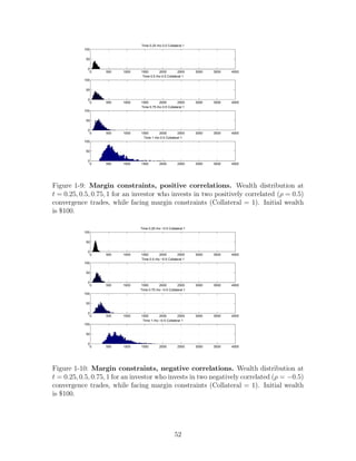
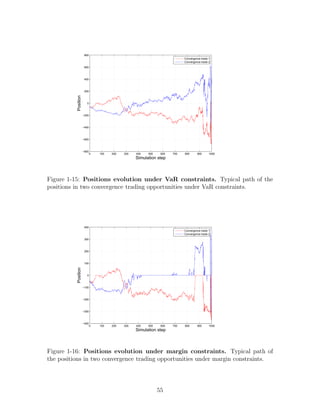
Figure 1-3: VaR constraints, positive correlations. Wealth distribution at t =
0.25, 0.5, 0.75, 1 for an investor who invests in two positively correlated (ρ = 0.5)
convergence trades, while facing VaR constraints (K=1). Initial wealth is $100.
0 500 1000 1500 2000 2500 3000 3500 4000
0
50
100
Time 0.25 rho −0.5 K 1
0 500 1000 1500 2000 2500 3000 3500 4000
0
50
100
Time 0.5 rho −0.5 K 1
0 500 1000 1500 2000 2500 3000 3500 4000
0
50
100
Time 0.75 rho −0.5 K 1
0 500 1000 1500 2000 2500 3000 3500 4000
0
50
100
Time 1 rho −0.5 K 1
Figure 1-4: VaR constraints, negative correlations. Wealth distribution at t =
0.25, 0.5, 0.75, 1 for an investor who invests in two negatively correlated (ρ = −0.5)
convergence trades, while facing VaR constraints (K=1). Initial wealth is $100.
48](https://image.slidesharecdn.com/938838223-mit-230323123641-6cde2771/85/938838223-MIT-pdf-48-320.jpg)


![• What does it mean to have a robust trading strategy?
A robust trading strategy is a strategy that works well over the set of alternative
probability models. We evaluate the worst performance of a given strategy over
that set of alternative probability models and we pick the one that maximizes
this worst case performance. It is essentially a “max-min” problem, a two-player
game in which a maximizing player chooses the best response to a malevolent
player who can disturb the stochastic model within limits.
• Why would we be interested in a robust decision rule over alternative models?
Why don’t we take a Bayesian approach, where we put a prior distribution over
the set of alternative probability models?
This could be another approach, but this set of alternative models may be too
large or too difficult for the investor to come up with a well behaved, plausible
prior distribution. In addition, we might want our solution to work well over
any kind of prior distribution [41].
• Why do we use the relative entropy to measure the discrepancy between an
alternative and the nominal model?
There are other ways to measure discrepancies between alternative probability
models, like Prokhorov distance [9] but the relative entropy with respect to a
measure P has nice properties and it is more tractable. It is given by:
D(Q) =
Z
log(
dQ
dP
)dQ
and it is a convex function of the measure Q.
In the rest of this chapter, we will review the relevant literature. Then we will
discuss about the set of the alternative models, the relative entropy and equivalent
ways to formulate our problem of the optimal robust portfolio allocation of the in-
vestor. Subsequently, we will find the optimal robust trading strategy of the investor
and finally we will explore the characteristics of this robust strategy.
58](https://image.slidesharecdn.com/938838223-mit-230323123641-6cde2771/85/938838223-MIT-pdf-58-320.jpg)
![2.1 Literature review
Whittle [79], [80] has studied mathematical methods for answering the question of
how to make decisions when you don’t fully trust your model.
Lars Hansen and Thomas Sargent in [41] have studied how to make economic
decisions in the face of model misspecification by modifying and extending aspects
of robust control theory. Their work revolves mostly around the linear-quadratic
regulator framework, where there is a certainty equivalence principle that allows a
deterministic presentation of the control theory.
Gilboa and Schmeidler in [34] have studied the max-min expected utility problem
where the decision maker has multiple priors and maximizes his expected utility as-
suming that nature chooses a probability measure to minimize his expected utility.
The minimization is over a closed and convex set of finitely additive probability mea-
sures. Their axiomatic treatment views this set of non-unique priors as an expression
of the agent’s preferences and the priors are not cast as distortions to a nominal
model.
Lars Hansen et al. [40] have studied robust decision rules when the agent fears that
the data are generated by a statistical perturbation of an approximating model that
is either a controlled diffusion process or a control measure over continuous functions
of time. They describe how stochastic formulations of robust control “constraint
problems” can be viewed in terms of Gilboa and Schmeidler’s max-min expected
utility model. They show the connection between the penalty robust control problem
and the constraint robust control problem, two closely related problems and formulate
the Hamilton Jacobi Bellman equations for various two-player zero sum continuous
time games that are defined in terms of a Markov diffusion process. We extend their
framework to the problem of optimal robust trading rules for a risk averse investor
who does not trust his model dynamics, believes that his nominal model is a good
approximation to the real model and invests in arbitrage opportunities.
Fleming and Souganidis [77] present how the Bellman-Isaacs condition defines a
Bellman equation for a two-player zero-sum game in which both players decide at time
59](https://image.slidesharecdn.com/938838223-mit-230323123641-6cde2771/85/938838223-MIT-pdf-59-320.jpg)
![0 or recursively. In other words, they show that the freedom to exchange orders of
maximization and minimization guarantees that equilibria of games where the choices
are done under mutual commitment at time 0 and of games where the choices are
done sequentially by both agents coincide.
Anderson et al. [3] show how the set of perturbed models in our formulations
is difficult to distinguish statistically from the approximating model given a finite
sample of timeseries observations.
Jacobson [44] and Whittle [78] studied risk sensitive optimal control in the context
of discrete-time linear quadratic regulator decision problems. They showed how the
risk-sensitive control law can be computed by equivalently solving a robust penalty
problem.
We will now discuss first how to represent the alternative probability models over
which we want our decision rules to be robust and how relative entropy can be used
to describe their discrepancies from the nominal model. We will formulate two closely
related nonsequential problems and the corresponding recursive HJB equations and
finally we will find the optimal robust portfolio allocation for a risk averse investor who
is not confident about the dynamics of his models and wants to invest in convergence
trades or mean reversion trading strategies.
2.2 Analysis
In Chapter 1 we saw that in the case when there is no model misspecification, the
investor wants to find the optimal portfolio allocation that solves the following prob-
lem:
maximizeθ∈Θ E(lnWT )
subject to
dWt = θtdSt + θ0tdBt
dSt = µ(S, t)dt + σ(S, t)dZt
dBt = rBdt
(2.1)
60](https://image.slidesharecdn.com/938838223-mit-230323123641-6cde2771/85/938838223-MIT-pdf-60-320.jpg)
![Here we have St ∈ RN
and we have studied the following special cases:
dSit = −
aiSit
T − t
dt +
K
X
k=1
σikdZkt
dSt = −Φ(St − S̄)dt + σdZt
and Θ is the set of admissible trading strategies:
Θ =
θ |θT
Σθ ≤ LW2
for the case of VaR constraints and
Θ =
(
θ |
N
X
i=1
λi|θi| ≤ W
)
for the case of the margin constraints.
In this Chapter, the investor doubts his model dSt = µ(S, t)dt + σ(S, t)dZt. To
capture this doubt of the investor, we surround the approximating model with a cloud
of models that are statistically difficult to distinguish and we add a malevolent agent
who picks the worst possible model. The investor wants to find the optimal trading
strategy that solves the following problem:
maxθ∈Θ minQ∈Q EQ(lnWT ) (2.2)
where Θ is the set of admissible trading strategies and Q is the set of alternative
probability models. Problem 2.2 fits the max-min expected utility model of Gilboa
and Schmeidler [34], where Q is a set of multiple different priors. Let’s now discuss
how we represent the set of alternative probability models.
2.2.1 Alternative models representation
We use martingales to represent perturbations to the probability models and relative
entropy to measure the discrepancy between our nominal model and the alternative
61](https://image.slidesharecdn.com/938838223-mit-230323123641-6cde2771/85/938838223-MIT-pdf-61-320.jpg)
![models. To understand better our continuous time formulations, we digress for a
while by borrowing an example from [41].
Let’s consider a discrete time approximating model and its innovations ǫt which are
i.i.d Gaussian shocks. An alternative model alters the distribution of these shocks.
We use martingales to represent distortions to the probabilities. Let π̂t(ǫ) be the
alternative density of the shock ǫt+1 based on date t information. Then the random
variable Mt =
Qt
j=1 mj, where mj =
π̂j−1(ǫ)
π(ǫ)
and M0 = 1, is a martingale and is a
ratio of the joint alternative density over the joint nominal density. We define the
entropy of the alternative distribution associated with Mt as the expected likelihood
ratio with respect to the distorted distribution E(Mtlog(Mt)). It has the property
that it is always non-negative and it is equal to 0, only when there is no distortion to
the nominal distribution.
Similarly, in our continuous time formulations we will use martingales to represent
distortions to the nominal probability model. We will construct an alternative model
by replacing Zt in our model by Ẑt +
R t
0
hsds, where Ẑt is a Brownian motion under the
alternative measure Q and ht is an adapted process that models the distortion, such
that the process ξt = e
R t
0
hsdZs− 1
2
R t
0
hT
s hsds
is a martingale. Therefore, the nominal model
is misspecified by allowing the conditional mean of the shock vector in the alternative
models to feed back arbitrarily on the history up to date t. Since ξ0 = 1 we have
that E(ξt) = 1. Since in addition, ξt 0, we can define a probability measure Q such
that Q(A) = E[1AξT ], in other words ξT = dQ
dP
is the Radon-Nikodym derivative of
Q with respect to P, where the measures Q and P are equivalent. In fact one can
always define a process ht so that for any measure Q the Radon-Nikodym derivative
of Q with respect to P, dQ
dP
, is given by the exponential martingale ξT . In this way,
our distorted models are:
• For the convergence trades,
dSt = −
aiSit
T − t
dt +
K
X
k=1
σik(dẐkt + hktdt) (2.3)
62](https://image.slidesharecdn.com/938838223-mit-230323123641-6cde2771/85/938838223-MIT-pdf-62-320.jpg)
![• For the mean reversion trades,
dSt = −Φ(St − S̄)dt + σ(dẐt + htdt) (2.4)
where Ẑt is a Brownian motion under Q. Why is it a Brownian motion under Q? The
answer lies with the Girsanov theorem [30] that states that if a process ht is such that
ξt is a martingale and ξT = dQ
dP
is the Radon-Nikodym derivative of Q with respect
to P, then the process ˆ
Z(t) = Zt −
R t
0
hsds is a Brownian motion under measure Q.
Therefore, we parameterize Q by the choice of the drift distortion adapted process
ht.
Similarly with the discrete time case, we measure the discrepancy between mea-
sures Q and P as the relative entropy D(Q) (see Appendix for derivation),
D(Q) =
Z T
0
1
2
EQ[hT
t ht]dt (2.5)
.
This is to be expected, since the relative entropy between a multivariate Gaussian
distribution N(µ, I) and the multivariate standard normal distribution is D(Q) =
1
2
µT
µ (See Appendix for derivation) and htdt is the conditional mean of the process
dZt under the alternative probability measure Q.
To express the notion that the nominal model is a good approximation to the real
model that generate the spread dynamics, we either restrain the alternative models
by D(Q) ≤ η or we penalize them with the magnitude of the entropy.
2.2.2 Model setup
Having described the set of alternative distributions, we are ready to formulate the
problem a risk averse investor faces who distrusts his model dynamics. As in [40] we
define two closely related problems:
63](https://image.slidesharecdn.com/938838223-mit-230323123641-6cde2771/85/938838223-MIT-pdf-63-320.jpg)
![• A multiplier robust control problem.
maxθ∈Θ minQ EQ(lnWT ) + νD(Q)
subject to dWt = θtdSt + θ0tdBt
dSt = µ(S, t)dt + σ(S, t)(dẐt + htdt)
dBt = rBdt
dξt = ξthtdZt
(2.6)
where ξT = dQ
dP
and D(Q) is given by equation 2.5. Here in essence there is an
implicit restriction manifested by the nonnegative penalty parameter ν.
• A constrained robust control problem.
maxθ∈Θ minQ EQ(lnWT )
subject to dWt = θtdSt + θ0tdBt
dSt = µ(S, t)dt + σ(S, t)(dẐt + htdt)
dBt = rBdt
dξt = ξthtdZt
D(Q) ≤ η
(2.7)
where ξT = dQ
dP
and D(Q) is given by equation 2.5.
In both cases the minimizing malevolent agent chooses the distortion process ht taken
θ as given and the maximizing investor chooses the optimal strategy taken ht as given.
We index the family of multiplier robust control problems by ν and the family of
constrained robust control problems by η. Obviously the two problems are related,
since the robustness parameter ν can be interpreted as the Lagrange multiplier on
the constraint D(Q) ≤ η. Actually we can show that if V (ν) is the optimal value
of the multiplier robust problem and K(η) is the optimal value of the constrained
robust problem then we have: K(η) = maxν≥0V (ν) − νη [40]. Therefore we will be
only interested in finding V (ν).
64](https://image.slidesharecdn.com/938838223-mit-230323123641-6cde2771/85/938838223-MIT-pdf-64-320.jpg)
![2.3 Solution
We will solve 2.6 by solving the corresponding Hamilton Jacobi Bellman (HJB) equa-
tion. We will solve the HJB equation for the case that there are no constraints in
the admissible trading strategies and when the trading strategies are constrained by
VaR or collateral considerations. But first let’s digress for a while and solve the HJB
equation for the case when there is no fear of model misspecification.
2.3.1 No fear of model misspecification
For now we assume that the investor completely trusts the dynamics of his models
dSt = µ(S, t)dt + σ(S, t)dZt. He chooses the trading strategy θ ∈ Θ that solves the
problem 2.1 where Θ is the set of admissible trading strategies:
Θ =
θ|θT
Σθ ≤ LW2
for the case of VaR constraints and
Θ =
(
θ|
N
X
i=1
λi|θi| ≤ W
)
for the case of the margin constraints. In this case the HJB equation is:
max
θ∈Θ
Vt + VW (Wr + θT
(µ(S, t) − rSt)) + V T
S µ(S, t)
+ 1/2VW W θT
Σθ + VW SΣθ + 1/2trace(ΣVSS) = 0
where Σ = σσT
and V (W, S, t) is the value function of the investor subject to the
terminal condition V (W, S, T) = ln(W).
Due to the logarithmic preferences of the investor it is: V (W, S, t) = ln(W)+H(S, t),
therefore VW S = 0, VW = 1
W
and VW W = − 1
W 2 . We also define ∀t ∈ [0, T] Ft = θt/Wt
∈ RN
.
65](https://image.slidesharecdn.com/938838223-mit-230323123641-6cde2771/85/938838223-MIT-pdf-65-320.jpg)

![2.3.2 Fear of model misspecification no constraints
In this section we assume that there are no constraints in the trading strategies fol-
lowed by the risk averse investor and the investor is not confident about the dynamics
of his models. The Hamilton Jacobi Bellman equation for the problem 2.6 is given
by:
max
θ
min
h
Vt + VW (Wr + θT
(µ(S, t) − rSt)) + V T
S µ(S, t)
+ 1/2VW W θT
Σθ + VW SΣθ + 1/2trace(ΣVSS) + VW θT
σh + V T
S σh +
ν
2
hT
h = 0
where Σ = σσT
and V (W, S, t) is the value function of the investor subject to the
terminal condition V (W, S, T) = ln(W). The malevolent agent picks the worst case
distortion drift process ht and the investor maximizes against the worst case scenario.
After defining ∀t ∈ [0, T] Ft = θt/Wt ∈ RN
the HJB equation becomes:
max
F
min
h
Vt + WVW (r + FT
(µ(S, t) − rSt)) + V T
S µ(S, t)
+1/2W2
VW W FT
ΣF+WVW SΣF+1/2trace(ΣVSS)+WVW FT
σh+V T
S σh+
ν
2
hT
h = 0
The inner minimization problem is a convex quadratic problem. The first order
conditions are:
WVW σT
F + σT
VS + νh = 0
h = −
σT
(WVW F + VS)
ν
The optimal value of the inner minimization problem is:
g(F) = −
W2
V 2
W Ft
ΣF + V T
S ΣVS + 2WVW FT
ΣVS
2ν
67](https://image.slidesharecdn.com/938838223-mit-230323123641-6cde2771/85/938838223-MIT-pdf-67-320.jpg)


![A little more thought though will exclude the last two cases, since we expect the value
function V to be a non-decreasing function of S for nonnegative values of the spread,
since higher values of the spread S correspond to better investment opportunities.
That will lead to non-negative values of VS for S ≥ 0.
The HJB equation is given by:
Vt + r + 1/2 σ2
VSS + 1/2
1
1 + 1
ν
(
a
T − t
+ r)2 S2
σ2
+ VS(−
a
T − t
S +
( a
T−t
+ r)S
ν + 1
) − 1/2
1
ν + 1
V 2
S σ2
= 0
We solve the HJB equation numerically using the method of finite differences [75].
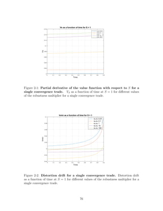
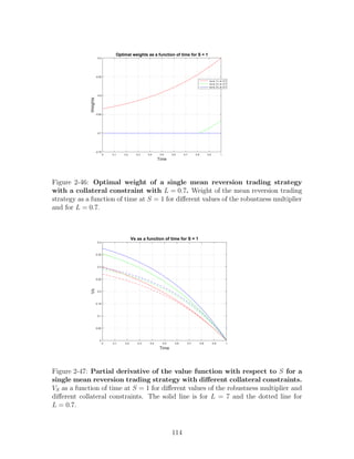
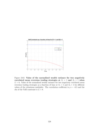
In the following figures we have assumed that rf = 0, σ = 1, a = 0.01 and T = 1.
We observe the following:
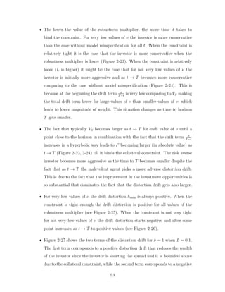
• VS becomes larger and larger as t → T for each value of ν as we see in Figure 2-1
until some value close to the horizon where it starts going down. In addition,
VS is higher for higher values of ν.
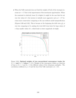
• For very low values of ν the drift distortion hmin is positive and becomes larger
as t → T as we see in Figure 2-2. For higher values of ν the drift distortion
starts negative and after some point increases as t → T to positive values. As we
showed in the previous section, when hmin = 0, the optimal weight is equal to
the optimal weight in the case where there is no fear of model misspecification.
We can see this in Figure 2-4, where very close at the time where hmin crosses
0, the optimal weight graph crosses the one when ν = 100.
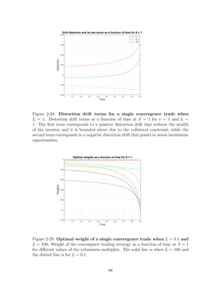
• Figure 2-3 shows the two terms of the distortion drift for ν = 1. The first term
corresponds to a positive distortion drift that reduces the wealth of the investor
since the investor is shorting the spread, while the second term corresponds to
a negative distortion drift that points to worse investment opportunities. In
this tradeoff the first term is losing at the beginning which makes the drift
distortion negative but as t → T it increases in a fast rate making the drift
distortion positive.
74](https://image.slidesharecdn.com/938838223-mit-230323123641-6cde2771/85/938838223-MIT-pdf-74-320.jpg)


![Chapter 3
Estimating the NIH Efficient
Frontier
The National Institutes of Health (NIH) is among the world’s largest and most im-
portant investors in biomedical research. Its stated mission is to “seek fundamental
knowledge about the nature and behavior of living systems and the application of
that knowledge to enhance health, lengthen life, and reduce the burdens of illness
and disability” (http://www.nih.gov/about/mission.htm). Some have criticized the
NIH funding process as not being sufficiently focused on disease burden[69, 45, 43].
We consider a framework in which biomedical research allocation decisions are
more directly tied to the risk/reward trade-off of burden-of-disease outcomes. Pri-
oritizing research efforts is analogous to managing an investment portfolio—in both
cases, there are competing opportunities to invest limited resources, and expected
returns, risk, correlations, and the cost of lost opportunities are important factors in
determining the return of those investments.
Financial decisions are commonly made according to portfolio theory[55], in which
the optimal trade-off between risk and reward among a collection of competing
investments—known as the “efficient frontier”—is constructed via quadratic opti-
mization, and a point on this frontier is selected based on an investor’s risk/reward
preferences. Given a measure of “return on investment” (ROI), an “efficient portfo-
lio” is defined to be the investment allocation that yields the highest expected return
131](https://image.slidesharecdn.com/938838223-mit-230323123641-6cde2771/85/938838223-MIT-pdf-131-320.jpg)
![for a given and fixed level of risk (as measured by return volatility), and the locus of
efficient portfolios across all levels of risk is the efficient frontier.
We recast the NIH funding allocation decision as a portfolio-optimization problem
in which the objective is to allocate a fixed amount of funds across a set of disease
groups to maximize the expected “return on investment” (ROI) for a given level of
volatility. We define ROI as the subsequent improvements in years of life lost (YLL).
We use historical time series data provided by the NIH and the Centers for Disease
Control for each of 7 disease groups and we estimate the means, variances, and co-
variances among these time series. These serve as inputs to the portfolio-optimization
problem. Such an approach provides objective, systematic, transparent, and repeat-
able metrics that can incorporate “real-world” constraints, and yields well-defined
optimal risk-sensitive biomedical research funding allocations expressly designed to
reduce the burden of disease.
In the rest of this chapter, we will discuss the relevant literature review. Then
we will discuss about the data and solution methods used, present our results and
conclude with a discussion of our findings.
3.1 NIH Background and Literature Review
The National Institutes of Health (NIH) was established in 1938 and has a budget
of over $31 billion, of which 80% is awarded in competitive research grants to more
than 325,000 researchers through nearly 50,000 competitive grants at over 3,000 uni-
versities, medical schools, and other research institutions (http://www.nih.gov). The
NIH allocates funding among competing priorities by assessing such priorities with re-
spect to five major criteria[65]: (a) public needs; (b) scientific quality of the research;
(c) potential for scientific progress (the existence of promising pathways and qualified
investigators); (d) portfolio diversification; and (e) adequate support of infrastruc-
ture (human capital, equipment, instrumentation, and facilities). This framework
was supported, with some additional recommendations, by an Institute of Medicine
(IoM) blue-ribbon panel in 1998 (see Table 3.1)[1].
132](https://image.slidesharecdn.com/938838223-mit-230323123641-6cde2771/85/938838223-MIT-pdf-132-320.jpg)

![Despite this framework and the IoM endorsement, NIH funding has been criticized
as not being aligned to disease burden and insufficiently effective[69, 45, 43]. For
example, the impact of cancer has been estimated as only 5% of total direct cost but
23% of all deaths[20], while extramural spending by the National Cancer Institute
(NCI) is about 15% of the total (http://report.nih.gov/). Sandler et al.[70] suggested
that digestive diseases were relatively underfunded based on comparisons of disease
burden as measured by direct and indirect cost. Gross[38] noted that NIH funding
is reasonably predicted by some burden-of-disease metrics (disability-adjusted life-
years or DALY, which are unavailable in time-series form)[57]. Earmarks or target
funding levels for specific diseases and programs have been suggested by a number of
policymakers[2].
Funding allocation decisions are not unique to the NIH; in a study similar to
Gross et al.Gross, Curry et al. [27] has questioned the allocations of the Centers
for Disease Control. NIH leaders have noted that funding basic research is itself a
risky endeavor, involving trade-offs among all five of their funding criteria, and may
also include unstated secondary objectives, e.g., actively “balancing out” spending by
other agencies, charities, and the private sector[76]. Collectively, these factors impose
significant challenges to determining an ideal allocation of research funds.
Although the economic impact of biomedical research has been considered[23],
the main focus has been on measuring value-added rather than determining optimal
funding allocations. Murphy and Topel [63] estimate U.S. economic surplus from
improved health on the order of $2.6 trillion annually, with benefits distributed un-
equally across age and gender, and suggest that in some cases, incremental benefits
may not exceed the cost of achieving them. Johnston et al.[46] found a return to soci-
ety in the form of averted treatment costs and public health benefits divided by cost
of trial expenditures of 46% for clinical trials at the National Institute of Neurological
Disorders and Stroke (NINDS), where the returns or net savings were generated by
four of the 28 trials examined, and collectively exceeded the costs of not only the
clinical, but the entire program of research at NINDS during the study period. Cut-
ler and McClellan[28] computed returns of technological advances for five conditions
134](https://image.slidesharecdn.com/938838223-mit-230323123641-6cde2771/85/938838223-MIT-pdf-134-320.jpg)
![and found net benefit for four and costs equal to benefits in the fifth. Fleurence and
Togerson[31] suggested that research should be allocated to provide the most health
benefits to the population, subject to equity considerations, and observed that sub-
jective, burden-of-disease, and payback methods all failed this test to some degree.
Instead, they argue that a method of information valuation is superior.
Modern financial portfolio theory—in which the expected return, risk (as measured
by volatility), and correlations of a collection of investment opportunities are taken
as inputs, and the set of all portfolio weights with the highest expected return for
a given level of risk is the output—produces rational allocations of limited resources
among competing priorities. For developing this method in 1952, Markowitz shared
the Nobel Memorial Prize in Economic Sciences in 1990. The theory has had extensive
applications among mutual funds, pension funds, endowments, and sovereign wealth
funds[55, 56, 24].
More recently, portfolio theory has been proposed as a means for conducting risk-
sensitive cost-benefit analysis for health-care budgeting decisions[11, 66, 19, 18, 71,
72]. The motivation for these studies is the observation that typical cost-effectiveness
studies of healthcare programs ignore the uncertainty of realized costs, which can be
addressed by applying portfolio theory to balance the risks against the rewards of spe-
cific budget allocations. These studies present simplified frameworks for incorporating
risk into the healthcare budgeting process, e.g., two-security examples (although[71]
does contain 11 hypothetical cost/effect distributions) and do not contain full-scale
empirical applications to realistic budgeting tasks. As the authors note, applying
portfolio theory to large public healthcare reimbursement problems can be challeng-
ing. Patients may have differing and non-constant utility functions, and some argue
that the manager/administrator should only consider expected returns, allowing the
patient and physician to consider risk trade-offs at individual treatment levels, in
which case the aggregate utility function is implicit.
Despite the growing interest in measuring the return on biomedical research[67,
51], and the fact that portfolio theory has already been applied to healthcare bud-
geting decisions, some sceptics continue to argue against the use of any quantita-
135](https://image.slidesharecdn.com/938838223-mit-230323123641-6cde2771/85/938838223-MIT-pdf-135-320.jpg)
![tive metrics in this domain. For example, Black[14] states categorically that “[t]he
biomedical ‘payback’ approach is certainly inappropriate and attempts to impose it
should be strenuously resisted. Instead, a qualitative approach should be applied
that takes into account the ‘slow-burning fuse’ and avoids simple attribution of cause
and effect”. While such a response may be acceptable for certain types of funding,
it is becoming increasingly untenable with respect to public funds and government
support, which, by law, almost always require some form of cost/benefit analysis,
performance attribution, and oversight.
3.2 Methods
3.2.1 Funding Data
The NIH has 27 Institutes and Centers, of which we identified 10 with research
missions clearly tied to specific disease states, and which account for $21 billion of
funding in 2005 or 74% of the total (see Table 3.2 for the disease classification scheme
used and Figure 3-1 for the procedure for constructing the appropriation time series).
The National Institute of Allergies and Infectious Diseases (NIAID) spending has
been split to account for HIV, which is presented separately (see HIV discussion
below).
These Institutes and the basic research they fund have inevitable overlap and
effect beyond their charter; we treat all spending for any given Institute as being
directed toward the corresponding disease states, and account for spillover effects by
considering the correlations in the lessening of the burden of disease in other groups.
For example, molecular biology funded by the NCI may be relevant to infectious
diseases but, like the entire NCI budget, would be assumed for modeling purposes to
be directed at cancer; the hypothetical infectious-disease improvement would appear
in the correlation between the decrease in years of life lost for cancer and that of
infectious diseases.
136](https://image.slidesharecdn.com/938838223-mit-230323123641-6cde2771/85/938838223-MIT-pdf-136-320.jpg)


![from other domestic and international medical centers and institutes, spending in
the pharmaceutical and biotechnology industries, public health policy, behavioral
patterns, prosperity level and environmental conditions. Therefore, the YLL/NIH-
funding relation is likely to be noisy, with confounding effects that may not be easily
disentangled. The Discussion section contains a more detailed discussion of this
assumption and some possible alternatives.
The second issue is the significant time lag between research expenditures and
observable impact on YLL. For example, Mosteller[62] cites a lag of 264 years, starting
in 1601, for the adoption of citrus to prevent scurvy by the British merchant marine.
More contemporary examples[26, 35, 39] cite lags of 17 to 20 years. We use shorter
lags in this study both because of data limitations (our entire dataset spans only
29 years), and also to reduce the impact of factors other than research expenditures
on our measure of burden of disease (YLL). Any attempt to optimize appropriations
to achieve YLL-related objectives must take this lag into account, otherwise the
resulting optimized appropriations may not have the intended effects on subsequent
YLL outcomes.
The impact of NIH-funded research on disease burden is likely to be spread out
over several years after this intervening lag, given the diffusion-like process in which
research results are shared in the scientific community. For simplicity, the same
duration (p = 5 years) of the diffusion-like impact for all the disease groups was
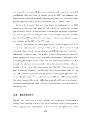
hypothesized. The lag q for each disease group was estimated by running linear
regressions associating improvements in YLL over p = 5 years with NIH funding q
years earlier and real income and choosing the lag between 9 and 16 years ( beyond
which data limitations and other factors make it impossible to distinguish the impact
of research funding from other confounding factors affecting YLL) that maximizes
the R2
and the corresponding lags are shown in Table 3.3.
This procedure is, of course, a crude but systematic heuristic for relating research
funding to YLL outcomes. Alternatives include using a single fixed lag across all
groups, simply assuming particular values for group-specific lags based on NIH man-
dates and experience, computing a time-weighted average YLL for each group with
143](https://image.slidesharecdn.com/938838223-mit-230323123641-6cde2771/85/938838223-MIT-pdf-143-320.jpg)
![a weighting scheme corresponding to an assumed or estimated knowledge-diffusion
rate for that group, or constructing a more accurate YLL return series by tracking
individual NIH grants within each group to determine the specific impact on YLL
(through new drugs, protocols, and other improvements in morbidity and mortality)
from the award dates to the present. While the choice of lag is critical in determining
the characteristics of the YLL return series and deserves further research, it does
not effect the applicability of the overall analytical framework. While our procedure
is surely imperfect, it is a plausible starting point from which improvements can be
made.
Assuming constant impact of research funding on YLL over the duration of p
years, the measure of the ROI that accrues to funds allocated in year t is then given
by:
Rt+q ≡ −
1
p
Pp−1
i=0 (YLLt+q+i − YLLt+q+i−1) × GDPt+q+i
Appropriationt
(3.2)
where the minus sign reflects the focus on decreases in YLL, and the multiplier
GDPt+q is per capita real gross domestic product (GDP) in year t+ q , which is
included to convert the numerator to a dollar-denominated quantity to match the
denominator. This ratio’s units are then comparable to those of typical investment
returns: date-(t+q) dollars of return per date-t dollars of investment.
Given the definition in equation (3.2) for the ROI of each of the disease groups,
the “optimal” appropriation of funds among those groups must be determined, i.e.,
the appropriation that produces the best possible aggregate expected return on total
research funding per unit risk. Denote by R ≡ [ R1 R2 · · · Rn ]′
the vector
of returns of all n groups for a given appropriation date t (where time subscripts
have been suppressed for notational simplicity), and denote by µ and Σ the vector
of expected returns and the covariance matrix, respectively. If the weights of the
budget allocation among the groups are ω, the ROI for the entire portfolio of grants,
denoted by Rp, is given by Rp = ω′
R, and its expected value and variance are ω′
µ
and ω′
Σω, respectively. The objective function to be optimized is then given by
144](https://image.slidesharecdn.com/938838223-mit-230323123641-6cde2771/85/938838223-MIT-pdf-144-320.jpg)

![where ι is an (n × 1)-vector of 1’s and µo is an arbitrary fixed level of expected
return. By varying µo between a range of values and solving the optimization problem
for each value, all the efficient allocations ω∗
may be tabulated, and the locus of
points in mean-standard-deviation space corresponding to these efficient allocations
is the efficient frontier. This so-called Markowitz portfolio optimization problem
involves minimizing a quadratic objective function with linear constraints, which is a
standard quadratic programming (QP) problem that can easily be solved analytically
in some cases[58], and numerically in all other cases by a variety of efficient and stable
solvers[37, 36].
One additional refinement to address the well-known issue of “corner solutions”
(in which several components of ω∗
are 0) that often arise in the standard portfolio-
optimization framework is proposed. While such extreme allocations may, indeed, be
optimal with respect to the mean-variance criterion, they are more often the result
of estimation error and outliers in the data[8]. Moreover, even in the absence of es-
timation error, mean-variance optimality may not adequately reflect other objectives
such as social equity across disease groups or distance from current status quo in al-
location. To incorporate such considerations, a “regularization” technique is applied
in which the objective function is penalized for allocations that are far away from the
average allocation policy. Specifically, we consider the following regularized version
of the standard portfolio-optimization problem:
Minimize
ω
ω′
Σω + γ kω − ωNIHk2
subject to ω′
µ ≥ µo , ω′
ι = 1 , ω ≥ 0
(3.4)
This formulation is essentially a dual-objective optimization problem in which the
first objective is to minimize the portfolio’s variance (ω′
Σω), and the second objective
is to minimize the difference from the average NIH allocation policy (kω − ωNIHk2
)
and the non-negative parameter γ determines the relative importance of these two
objectives. Larger values of γ yield optimal weights that are closer to average NIH al-
146](https://image.slidesharecdn.com/938838223-mit-230323123641-6cde2771/85/938838223-MIT-pdf-146-320.jpg)


![suggest that significant YLL improvements with respect to a mean-variance criterion
may be possible through funding re-allocation. To our knowledge, this is the first
time such an approach has been empirically implemented in this domain.
However, our findings must be qualified in at least three respects: (1) YLL as a
measure of burden of disease, which is clearly incomplete and less than ideal; (2) the
definition of ROI and the challenges of relating research expenditures to subsequent
outcomes such as burden of disease; and (3) the known limitations of portfolio the-
ory. While each of these qualifications can be addressed to varying degrees through
additional data and analysis, the empirical conclusions are likely to depend critically
on the nature of their resolution. In this section, we provide a short synopsis of these
qualifications, and also consider other objections to this framework and directions for
future research.
YLL captures only the most extreme form of disease burden, and other measures
such as disability-adjusted or quality-adjusted life years are clearly preferable. How-
ever, time series histories for such measures are currently unavailable; hence YLL is
the most natural starting point for gauging the impact of biomedical research funding,
and is directly aligned with the NIH mission to “lengthen life”.
As a measure of disease burden, YLL captures only lethal illness by definition;
chronic illness enters the optimization process only indirectly, mortality in the young
is more heavily weighted than that of the elderly, and quality-of-life is not captured at
all. The choice of YLL is motivated by several factors: long time-series observations
of YLL are readily available, they cover a large population, and they address the
entire spectrum of diagnoses categorized under the ICD. Broader measures of burden
of disease such as disability adjusted life years (DALY)[38] and quality-adjusted life
years (QALY)[68, 22] have been proposed, but historical time series for such measures
are not yet available. As better measures are developed (e.g., incidence, prevalence,
physician visits, hospitalization, DALY, QALY), portfolio-optimization methods may
be applied to them as well through appropriately defined “returns”. Should datasets
covering not only age and cause of death but also ante-mortem symptoms become
available, mean-variance-efficient allocations would likely place significant weight on
152](https://image.slidesharecdn.com/938838223-mit-230323123641-6cde2771/85/938838223-MIT-pdf-152-320.jpg)
![improvements in the care of less-lethal chronic diseases.
Even if YLL is an appropriate measure of disease burden, our definition of ROI
can also be challenged as being imprecise and ad hoc in several respects. NIH funding
is typically focused on basic research rather than translational efforts, therefore, NIH
spending may not be as directly related to subsequent YLL improvements. We have
not accounted for other expenditures that may also affect YLL, and to the extent
that NIH appropriations are systematically used to complement private spending
to allocate total funding across diseases more fairly[76], the relation between NIH
funding and subsequent YLL improvements may be even noisier, and may require
modelling private-sector expenditures as a separate but complementary portfolio-
optimization problem with an objective function and constraints that are linked to
those of the NIH. Also, the standard portfolio-optimization framework implicitly as-
sumes a constant multiplicative relation between dollars invested today and dollars
returned tomorrow (so that doubling the investment will typically double the ROI of
that investment), whereas the return to biomedical investments may be non-linear.
In addition, translational research takes time and significant non-NIH resources, fur-
ther blurring the relation between NIH allocations and subsequent changes in YLL.
Finally, other factors may contribute to YLL improvements, including changes in cul-
tural norms (including consumption of alcohol and cigarettes), economic conditions
(such as recessions vs. expansions), and public policy (such as vaccine programs and
mandates for automobile, home, and workplace safety). While all of these qualifica-
tions have merit, they are not insurmountable obstacles and can likely be addressed
through additional data collection and more sophisticated metrics, perhaps along the
lines of Porter[67] or Lane and Bertuzzi[51]. Moreover, the portfolio-optimization
approach provides a useful conceptual framework for formulating funding allocation
decisions systematically, even if its empirical implications are imprecise.
The estimates of q were an initial attempt to link appropriation with outcome in
a systemic and non-discretionary manner, but they were derived heuristically from
regulatory, appropriation, and epidemiological data which may not be stationary or
predictive. For example, if the Food and Drug Administration’s capacity for reviewing
153](https://image.slidesharecdn.com/938838223-mit-230323123641-6cde2771/85/938838223-MIT-pdf-153-320.jpg)
![new-drug applications is held constant and applications double, substantial increases
in regulatory queuing would be expected, even with the added resources generated by
the Prescription Drug User Fee Act. Finally, in converting changes in YLL to dollar
amounts, per-capita real GDP was used as the “conversion factor” irrespective of age,
despite the fact that children and retired individuals are economically less active.
While these caveats highlight the imprecision with which the impact of research
spending is measured, they also provide direction for developing better metrics. In
particular, the underlying science of each grant implies a particular set of dynamics for
translation and YLL impact, and with more sophisticated models of such dynamics,
the returns to fundamental research should be measurable with greater accuracy.
Even within the exact domain for which it was developed, portfolio theory has
several well-known limitations, of which the most obvious is the possibility that the
mean-variance criterion may not, in fact, be the appropriate objective function to
be optimized. While there is little disagreement that higher expected ROI is prefer-
able to its alternative, the trade-off between expected ROI and risk is fraught with
subtleties involving specific psychological, perceptual, and behavioural mechanisms
of individuals and groups. Because of these considerations, mean-variance analysis is
often considered an approximation to a much more complicated reality—a starting
point for investment allocation decisions, not the final answer.
Another known limitation of portfolio theory is the fact that the input parameters
(µ, Σ) must be estimated from historical data, and estimation error in these param-
eter estimates can lead to portfolios that are unstable and sub-optimal[55]. One
common approach to addressing this problem in the financial context is to employ
prior information regarding the input parameters, thereby reducing the dependence
on historical data. Using Bayesian methods, expert opinions regarding the statisti-
cal properties of the individual asset returns can be incorporated into the portfolio
optimization process[13, 5] [12].
One limitation that is unique to the current application is the fact that portfolio
theory is silent on which mean-variance-optimal portfolio to select. In the financial
context, the existence of a riskless investment (e.g., U.S. Treasury bills) implies that
154](https://image.slidesharecdn.com/938838223-mit-230323123641-6cde2771/85/938838223-MIT-pdf-154-320.jpg)
![one unique portfolio on the efficient frontier will be desired by all investors—the so-
called “tangency” portfolio[73]. Because there is no analog to a riskless investment in
biomedical research, the notion of a tangency portfolio does not exist in this context.
Therefore, decision makers must first determine society’s collective preferences for risk
and return with respect to changes in YLL before a unique solution to the portfolio-
optimization problem can be obtained, i.e., they must agree on a societal “utility
function” for trading off the risks and rewards of biomedical research.
This critical step is a pre-requisite to any formal analysis of funding allocation
decisions, and underscores the need for integration of basic science with biomedical
investment performance analysis and science policy. Such integration will require
close and ongoing collaboration between scientists and policymakers to determine the
appropriate parameters for the funding allocation process, and to incorporate prior
information and qualitative judgments[14] regarding likely research successes, social
priorities, policy objectives and constraints, and hidden correlations due to non-linear
dependencies not captured by the data. In particular, it is easy to imagine contexts
in which funding objectives can and should change quickly in response to new envi-
ronmental threats or public-policy concerns. However, such pressing needs must be
balanced against the disruptions—which can be severe due to the significant adjust-
ment costs implicit in biomedical research[32]—caused by large unanticipated positive
or negative shifts in research funding. Although the end result of collaborative discus-
sion may fall short of a well-defined objective function that yields a clear-cut optimal
portfolio allocation, the portfolio-optimization process provides a transparent and ra-
tional starting point for such discussions, from which several insights regarding the
complex relation between research funding and social outcomes are likely to emerge.
Any repeatable and transparent process for making funding allocation decisions—
especially one that involves criteria other than peer-review-based academic excellence—
will, understandably, be viewed with some degree of suspicion and contempt by the
scientific community. However, if one of the goals of biomedical research is to reduce
the burden of disease, some tension between academics and public policy may be
unavoidable. Moreover, in the absence of a common framework for evaluating the
155](https://image.slidesharecdn.com/938838223-mit-230323123641-6cde2771/85/938838223-MIT-pdf-155-320.jpg)
![trade-offs between academic excellence and therapeutic potential, other approaches
such as political earmarking[2] are being proposed, which may be even less palatable
from the scientific perspective.
In an environment of tightening budgets and increasing oversight of appropria-
tions, portfolio theory offers scientists, policymakers, and regulators—all of whom
are, in effect, research portfolio managers—a rational, systematic, transparent, and
reproducible framework in which to explicitly balance and trade off expected benefits
with potential risks while accounting for correlation among multiple research agen-
das and real-world constraints in allocating scarce resources. Most funding agencies
and scientists have already been making such trade-offs informally and heuristically;
there may be additional benefits to making such decisions within an explicit frame-
work based on standardized and objective metrics.
One of the most significant benefits from adopting such a framework may be the
reduction of uncertainty surrounding future funding-allocation decisions, which would
greatly enhance the ability of funding agencies and scientists to plan for the future and
better manage their respective budgets, research agendas, and careers. By approach-
ing funding decisions in a more analytical fashion, it may be possible to improve their
ultimate outcomes while reducing the chances of unintended consequences.
156](https://image.slidesharecdn.com/938838223-mit-230323123641-6cde2771/85/938838223-MIT-pdf-156-320.jpg)

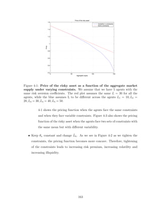
![agents and varying degrees of fear of model misspecification across agents. Finally,
we will conclude with all of our results.
4.1 Literature review
In the literature there are papers that assume heterogeneity along three dimensions:
risk aversion coefficients of the agents, constraints the agents face and beliefs of the
agents.
Danielsson and Zigrand [81] assume that the agents have the same beliefs and face
the same constraints but they differ in their risk aversion coefficients. They study
the economic implications of a Value-at-risk based regulatory system by analyzing a
two period multi-asset general equilibrium model with agents heterogeneous in risk
preferences and wealth. They assume that the agents have CARA utilities and they
argue that there will be endogenous volatility and increasing risk premium due to the
fact that “... risk will have to be transferred from the more risk-tolerant to the more
risk-averse”. As we will prove this is not true and not necessary for having increasing
risk premium, endogenous volatility and increasing illiquidity.
Kogan and Uppal [50] show how to analyze the equilibrium prices and policies in
an economy with incomplete financial markets and stochastic investment opportunity
set, where the agents face portfolio constraints. They study a general equilibrium
exchange economy with multiple agents, who differ in the risk aversion coefficients
and face borrowing constraints, while having the same beliefs.
Brumm et al. [21] consider a general equilibrium infinite-horizon economy with
the agents having heterogeneous risk preferences and facing the same constraints,
while having the same beliefs. They find that the presence of collateral constraints
leads to strong excess volatility and a regulation of margin requirements potentially
has stabilizing effects.
Then, there are papers with different prior beliefs not due to asymmetric infor-
mation among the agents. Geanakoplos [33] assumes that the agents have different
priors (optimists, pessimists) but same risk aversion coefficients and wealth and they
158](https://image.slidesharecdn.com/938838223-mit-230323123641-6cde2771/85/938838223-MIT-pdf-158-320.jpg)
![face identical collateral constraints. He studies how these constraints determine an
equilibrium leverage and how this leverage changes over time leading to crashes and
boom periods, the so-called leverage cycles.
Chen, Hong and Stein [25] study what happens to the price of a risky asset, when
there are investors with heterogeneous priors who face short sales constraints. The
idea that short sales constraints increase the prices of risky assets when the investors
have heterogeneous beliefs is due to Lintner [52] and Miller [61]. Chen, Hong and
Stein show that greater dispersion of beliefs leads to even higher prices.
Finally, Hansen and Sargent [41] study a framework where the agents have a
common approximating model, but they differ in the degree of mistrust of the model.
They find that agent’s caution in responding to concerns about model misspecification
can raise prices assigned to macroeconomic risks.
We will see how risk constraints affect the statistical properties of the market,
in particular the risk premium, volatility and liquidity of the market. We will first
study the case where the investors differ in the constraints they face and/or their risk
aversion coefficients and then the case where they mistrust the model of asset payoffs
and the mistrust varies among the investors.
4.2 Analysis
4.2.1 Model setup
We assume we have H mean-variance single-period optimizers with heterogeneous
risk aversions, risk constraints and wealth. Each agent can invest in the market and
the risk free rate at t = 0. We assume that the risk-free rate is exogenously given
and the market is modeled as a risky asset with stochastic payoff at t = 1. There are
also noise traders. We do not model their utility explicitly, we only assume that they
are hit by random liquidity shocks and they submit random market orders at time
t = 0. Equivalently, the supply of the risky asset is stochastic. Each agent faces a
risk constraint, a constraint in his wealth volatility of the form |θh| ≤ LhWh0, where
159](https://image.slidesharecdn.com/938838223-mit-230323123641-6cde2771/85/938838223-MIT-pdf-159-320.jpg)


![we have proved that:
Fopt
it =
sign(−µit)(|µit
λi
| − νopt
t )+
σ2
i
λi
Proposition 3. The relative entropy of a multivariate Gaussian distribution N(µ, I)
with respect to the multivariate standard Gaussian distribution is D(Q) = 1
2
µT
µ
Proof. It is:
D(Q) =
Z +∞
−∞
log(
f(x)
g(x)
)f(x)dx
where f(x) = 1
(2π)N/2 e−1/2(x−µ)T (x−µ)
and g(x) = 1
(2π)N/2 e−1/2xT x
D(Q) = −
Z +∞
−∞
1/2(x − µ)T
(x − µ)f(x)dx +
Z +∞
−∞
1/2xT
xf(x)dx
The first term is:
−
1
2
E[(X − µ)T
(X − µ)] = −
1
2
E[trace((X − µ)T
(X − µ))]
= −
1
2
E[trace((X − µ)(X − µ)T
)]
= −
1
2
trace(I)
= −N/2
The second term is:
1
2
E[XT
X] =
1
2
E[trace((X − µ)T
(X − µ))] +
1
2
E[X]T
E[X]
= N/2 +
1
2
µT
µ
Therefore, we have D(Q) = 1
2
µT
µ.
178](https://image.slidesharecdn.com/938838223-mit-230323123641-6cde2771/85/938838223-MIT-pdf-178-320.jpg)
![Proposition 4. The relative entropy of probability measure Q with respect to P,
where dQ
dP
= ξT and ξt = e
R t
0
hT
s dZs− 1
2
R t
0
hT
s hsds
is given by:
D(Q) =
Z T
0
1
2
EQ[hT
t ht]dt
Proof. The relative entropy of Q with respect to P is:
D(Q) = EQ[log(
dQ
dP
)]
= EQ[log(ξT )]
= EQ[
Z T
0
hT
s dZs −
1
2
Z T
0
hT
s hsds]
=
Z T
0
EQ[hT
s dZs] −
1
2
Z T
0
EQ[hT
s hs]ds
=
Z T
0
EQ[EQ[hT
s dZs|Fs]] −
1
2
Z t
0
EQ[hT
s hs]ds
=
Z T
0
1
2
EQ[hT
t ht]dt
since EQ[dZt|Ft] = htdt from Girsanov’s theorem.
Proposition 5. The following QCQP:
minimize −FT
(µ(S, t) − rSt −
ΣHS
ν
) +
1
2
(1 +
1
ν
)FT
t ΣFt
subject to FT
ΣF ≤ L
has a solution given by:
Fopt
t =
1
1+ 1
ν
Σ−1
µt if µT
t Σ−1
µt ≤ L(1 + 1
ν
)2
Σ−1µt
r
µT
t Σ−1µt
L
if µT
t Σ−1
µt ≥ L(1 + 1
ν
)2
where µt = µ(S, t) − rSt − ΣHS(St,t)
ν
.
Proof. Let us apply the Karush Kuhn Tucker (KKT) conditions. Fopt
t , λopt
t are optimal
iff they satisfy the following KKT conditions:
179](https://image.slidesharecdn.com/938838223-mit-230323123641-6cde2771/85/938838223-MIT-pdf-179-320.jpg)


![Bibliography
[1] Committee on the NIH Research Priority-Setting Process, Scientific Opportu-
nities and Public Needs: Improving Priority Setting and Public Input at the
National Institutes of Health, pp. 11–12. Washington, D.C.: National Academy
Press. (1998).
[2] C. Anderson. A new kind of earmarking. Science, 260(5107):483, Apr. 23, 1993
1993.
[3] Evan W. Anderson, Lars Peter Hansen, and Thomas J. Sargent. Robustness,
detection and the price of risk, 2000.
[4] Kerry E. Back. Asset Pricing and Portfolio Choice Theory. Oxford University
Press, 2010.
[5] Alexander Bade, Gabriel Frahm, and Uwe Jaekel. A general approach to Bayesian
portfolio optimization. Mathematical Methods of Operations Research, 70(2):337–
356, 2009.
[6] Suleyman Basak and B. Croitoru. Equilibrium mispricing in a capital market
with portfolio constraints. The Review of financial studies, 13:715–748, 2000.
[7] Suleyman Basak and Alexander Shapiro. Value-at-risk-based risk management:
Optimal policies and asset prices. The Review of financial studies, 14:371–405,
2001.
[8] V. Bawa, S. Brown, and R. Klein. Estimation Risk and Optimal Portfolio Choice.
North-Holland, Amsterdam, 1979.
[9] Dirk Bergemann and Karl Schlag. Robust monopoly pricing. Cowles Foundation,
Yale University, 2005.
[10] Dimitri P. Bertsekas. Convex Optimization Theory. Athena Scientific, 2009.
[11] S. Birch and A. Gafni. Cost effectiveness/utility analyses. Do current decision
rules lead us to where we want to be? Journal of Health Economics, 11:279–296,
1992.
[12] Dimitrios Bisias, Andrew W. Lo, and James F. Watkins. Estimating the NIH
efficient frontier. PLOS One, 2012.
183](https://image.slidesharecdn.com/938838223-mit-230323123641-6cde2771/85/938838223-MIT-pdf-183-320.jpg)
![[13] F. Black and R. Litterman. Global portfolio optimization. Financial Analysts
Journal, 48(5):28–43, 1992.
[14] Nick Black. Health services research: the gradual encroachment of ideas. Journal
of Health Services Research Policy, 14:120–123, 2009.
[15] Michael Boguslavsky and Elena Boguslavskaya. Arbitrage under power. Risk,
pages 69–73, June 2004.
[16] S. Boyd and L. Vandenberghe. Convex Optimization. Cambridge University
Press, Cambridge, UK, 2004.
[17] Michael J. Brennan and Eduardo S. Schwartz. Arbitrage in stock index futures.
The Journal of Business, 63, 1990.
[18] J. F. Bridges and D. D. Terris. Portfolio evaluation of health programs: A reply
to Sendi et al. Social Science Medicine, 58:1849–1851, 2004.
[19] J. F. B. Bridges, M. Stewart, M. T. King, and K. van Gool. Adapting portfolio
theory for the evaluation of multiple investments in health with a multiplicative
extension for treatment synergies. European Journal of Health Economics, 3:47–
53, 2002.
[20] M. L. Brown, J. Lipscomb, and C. Snyder. The burden of illness of cancer:
economic cost and quality of life. Annual Review of Public Health, 22:91–113,
2001.
[21] Johannes Brumm, Felix Kubler, Michael Grill, and Karl Schmedders. Margin
regulation and volatility. ECB working paper, 1698, 2014.
[22] Carol S. Burckhardt and Kathryn L. Anderson. The quality of life scale (QOLS):
Reliability, validity, and utilization. Health and Quality of Life Outcomes, 1:60–
66, 2003.
[23] M. Buxton, S. Hanney, and T. Jones. Estimating the economic value to societies
of the impact of health research: a critical review. Bulletin of the World Health
Organization, 82(10):733–739, Oct 2004.
[24] S. Chandra. Regional economy size and the growth/instability frontier: Evidence
from Europe. Journal of Regional Science, 43(1):95–122, 2003.
[25] Joseph Chen, Harrison Hong, and Jeremy C. Stein. Breadth of ownership and
stock returns. Journal of financial economics, 66:171–205, 2002.
[26] Julius H. Comroe Jr. and Robert D. Dripps. Scientific basis for the support of
biomedical science. Science, 192(4235):105–111, 1976.
[27] C. W. Curry, A. K. De, R. M. Ikeda, and S. B. Thacker. Health burden and
funding at the Centers for Disease Control and Prevention. American Journal
of Preventive Medicine, 30(3):269–276, MAR 2006.
184](https://image.slidesharecdn.com/938838223-mit-230323123641-6cde2771/85/938838223-MIT-pdf-184-320.jpg)
![[28] D. M. Cutler and M. McClellan. Is technological change in medicine worth it?
Health Affairs, 20(5):11–29, Sep–Oct 2001.
[29] Darrell Duffie. Special repo rates. Journal of Finance, 51:493–526, 1996.
[30] Darrell Duffie. Dynamic Asset Pricing Theory. Princeton Series in Finance, 3
edition, 2001.
[31] R. L. Fleurence and D. J. Torgerson. Setting priorities for research. Health
Policy, 69(1):1–10, JUL 2004.
[32] Richard Freeman and John Van Reenen. What if Congress doubled RD spend-
ing on the physical sciences? Technical Report 931, Center for Economic Per-
formance, May 2009.
[33] John Geanakoplos. The leverage cycle. Cowles Foundation Discussion Paper,
1715R, 2009.
[34] Itzhak Gilboa and David Schmeidler. Maxmin expected utility with non-unique
prior. Journal of Mathematical Economics, 18:141–153, 1989.
[35] J. Grant. Evaluating “payback” on biomedical research from papers cited in
clinical guidelines: applied bibliometric study. BMJ, 320(7242):1107–1111, 2000.
[36] M. Grant and S. Boyd. Graph implementations for nonsmooth convex programs.
In V. Blondel, S. Boyd, and H. Kimura, editors, Recent Advances in Learning and
Control (a tribute to M. Vidyasagar), Lecture Notes in Control and Information
Sciences, pages 95–110. Springer, Berlin / Heidelberg, 2008.
[37] M. Grant and S. Boyd. CVX: Matlab software for disciplined convex program-
ming, June 2009 2009.
[38] C. P. Gross, G. F. Anderson, and N. R. Rowe. The relation between funding
by the National Institutes of Health and the burden of disease. New England
Journal of Medicine, 340(24):1881–1887, JUN 17 1999.
[39] Steve Hanney, Iain Frame, Jonathan Grant, Philip Green, and Martin Buxton.
From Bench to Bedside: Tracing the Payback Forwards from Basic or Early
Clinical Research A Preliminary Exercise and Proposals for a Future Study.
Health Economics Research Group, Brunel University, Uxbridge, UK, 2003.
[40] Lars Hansen, Thomas Sargent, G. Turmuhambetova, and N. Williams. Robust
control, min-max expected utility and model misspecification. Journal of Eco-
nomic Theory, 128:45–90, 2006.
[41] Lars P. Hansen and Thomas Sargent. Robustness. Princeton University Press,
2008.
[42] Trevor Hastie, Robert Tibshirani, and Jerome Friedman. The Elements of Sta-
tistical Learning: Data Mining, Inference, and Prediction. Springer, 2013.
185](https://image.slidesharecdn.com/938838223-mit-230323123641-6cde2771/85/938838223-MIT-pdf-185-320.jpg)
![[43] Ernest Istook. Research funding on major diseases is not proportionate to tax-
payer’s needs. Journal of NIH Research, 9(8):26–28, 1997.
[44] D.H. Jacobson. Optimal stochastic linear systems with exponential performance
criteria and their relation to deterministic differential games. IEEE Transactions
Automatic Control, 18:124–131, 1973.
[45] S. C. Johnston and S. L. Hauser. Basic and clinical research: what is the most
appropriate weighting in a public investment portfolio? Annals of Neurology,
60(1):9A–11A, Jul 2006.
[46] S. C. Johnston, J. D. Rootenberg, S. Katrak, W. S. Smith, and J. S. Elkins.
Effect of a US national institutes of health programme of clinical trials on public
health and costs. Lancet, 367(9519):1319–1327, APR 22 2006.
[47] Philippe Jorion. Value at Risk: The New Benchmark for Managing Financial
Risk. McGraw-Hill, 2006.
[48] Jakub Jurek and Halla Yang. Dynamic portfolio selection in arbitrage. EFA
Meeting, 2006.
[49] Tong Suk Kim and Edward Omberg. Dynamic nonmyopic portfolio behavior.
The Review of Financial Studies, 9:141–161, 1996.
[50] Leonid Kogan and Raman Uppal. Risk aversion and optimal portfolio policies
in partial and general equilibrium economies. NBER working paper, 8609, 2001.
[51] Julia Lane and Stefano Bertuzzi. Measuring the results of science investments.
Science, 331:678–680, 2011.
[52] John Lintner. The aggregation of investor’s diverse judgements and preferences
in purely competitive security markets. Journal of financial and quantitative
analysis, 4:347–400, 1969.
[53] Jun Liu and Francis A. Longstaff. Losing money on arbitrage: Optimal dynamic
portfolio choice in markets with arbitrage opportunities. The Review of Financial
Studies, 17, 2004.
[54] Roger Lowenstein. When genius failed: The Rise and Fall of Long-Term Capital
Management. Random House Trade Paperbacks, 2001.
[55] H. M. Markowitz. Portfolio selection. Journal of Finance, 7(1):77–91, March
1952 1952.
[56] F. W. McFarlane. Portfolio approach to information systems. Harvard Business
Review, 59(4):142–150, 1981.
[57] M. T. McKenna, C. M. Michaud, C. J. L. Murray, and J. S. Marks. Assessing
the burden of disease in the United States using disability-adjusted life years.
American Journal of Preventive Medicine, 28(5):415–423, JUN 2005.
186](https://image.slidesharecdn.com/938838223-mit-230323123641-6cde2771/85/938838223-MIT-pdf-186-320.jpg)
![[58] Robert C. Merton. An analytic derivation of the efficient portfolio frontier.
Journal of Financial and Quantitative Analysis, 7:1851–1872, 1972.
[59] Robert C. Merton. Continuous time Finance. Wiley-Blackwell, 1992.
[60] Attilio Meucci. Review of statistical arbitrage, cointegration and multivariate
ornstein-uhlenbeck, 2010.
[61] Edward M. Miller. Risk, uncertainty and divergence of opinion. Journal of
Finance, 32:1151–1168, 1977.
[62] F. Mosteller. Innovation and evaluation. Science, 211(4485):881–886, 1981.
[63] Kevin Murphy and Richard Topel. Diminishing returns? The costs and benefits
of improving health. Perspectives in Biology and Medicine, 43(3):S108–S128,
2003.
[64] Rishi K. Narang. Inside the Black Box: A Simple Guide to Quantitative and
High Frequency Trading. Wiley, 2013.
[65] National Institutes of Health. Setting Research Priorities at the National Insti-
tutes of Health. National Institutes of Health, Bethesda, MD, 1997.
[66] B. J. O’Brien and M. J. Sculpher. Building uncertainty into cost-effectiveness
rankings: Portfolio risk-return tradeoffs and implications for decision rules. Med-
ical Care, 38:460–468, 2000.
[67] M. E. Porter. What is value in health care? New England Journal of Medicine,
363(26):2477–2481, 2010.
[68] Luis Prieto and Jose A. Sacristan. Problems and solutions in calculating quality-
adjusted life years (QALYs). Health and Quality of Life Outcomes, 1:80–87, 2003.
[69] S. J. Rangel, B. Efron, and R. L. Moss. Recent trends in National Institutes
of Health funding of surgical research. Annals of Surgery, 236(3):277–287, SEP
2002.
[70] R. S. Sandler, J. E. Everhart, M. Donowitz, E. Adams, K. Cronin, C. Goodman,
E. Gemmen, S. Shah, A. Avdic, and R. Rubin. The burden of selected digestive
diseases in the United States. Gastroenterology, 122(5):1500–1511, May 2002.
[71] P. Sendi, M. J. Al, A. Gafni, and S. Birch. Optimizing a portfolio of health
care programs in the presence of uncertainty and constrained resources. Social
Science Medicine, 57:2207–2215, 2003.
[72] Pedram Sendi, Maiwenn J. Al, and Frans F. H. Rutten. Portfolio theory and
cost-effectiveness analysis: A further discussion. Value In Health, 7:595–601,
2004.
187](https://image.slidesharecdn.com/938838223-mit-230323123641-6cde2771/85/938838223-MIT-pdf-187-320.jpg)
![[73] William F. Sharpe. Capital asset prices: a theory of market equilibrium under
conditions of risk. J. Finance, 19:425–442, 1964.
[74] Andrei Shleifer and Robert W. Vishny. The limits of arbitrage. The Journal of
Finance, 52:35–55, 1997.
[75] Gilbert Strang. Computational Science and Engineering. Wellesley Cambridge
Press, 2007.
[76] H. Varmus. Evaluating the burden of disease and spending the research dol-
lars of the National Institutes of Health. New England Journal of Medicine,
340(24):1914–1915, JUN 17 1999.
[77] W.H.Fleming and P.E.Souganidis. On the existence of value functions of two-
player zero-sum stochastic differential games. Indiana University Mathematics
Journal, 38:293–314, 1989.
[78] P. Whittle. Risk sensitive linear quadratic gaussian control. Advanced Applied
Probability, 13:776–777, 1981.
[79] P. Whittle. Risk sensitive optimal control. Wiley, 1990.
[80] P. Whittle. Optimal control: basics and beyond. Wiley, 1996.
[81] Jean-Pierre Zigrand and Jon Danielsson. What happens when you regulate risk?:
evidence from a simple equilibrium model. Lse research online documents on
economics, London School of Economics and Political Science, LSE Library, 2001.
188](https://image.slidesharecdn.com/938838223-mit-230323123641-6cde2771/85/938838223-MIT-pdf-188-320.jpg)