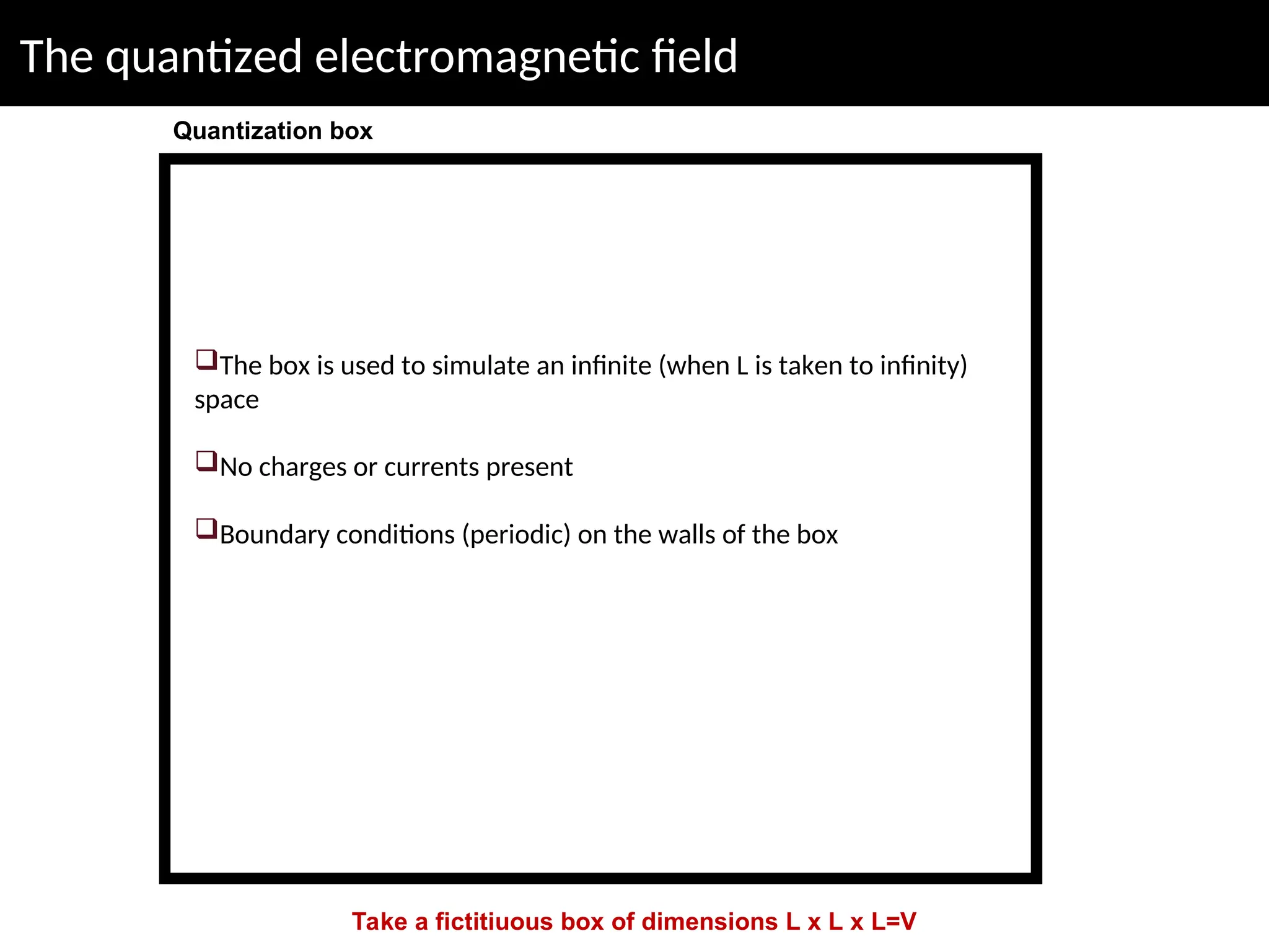
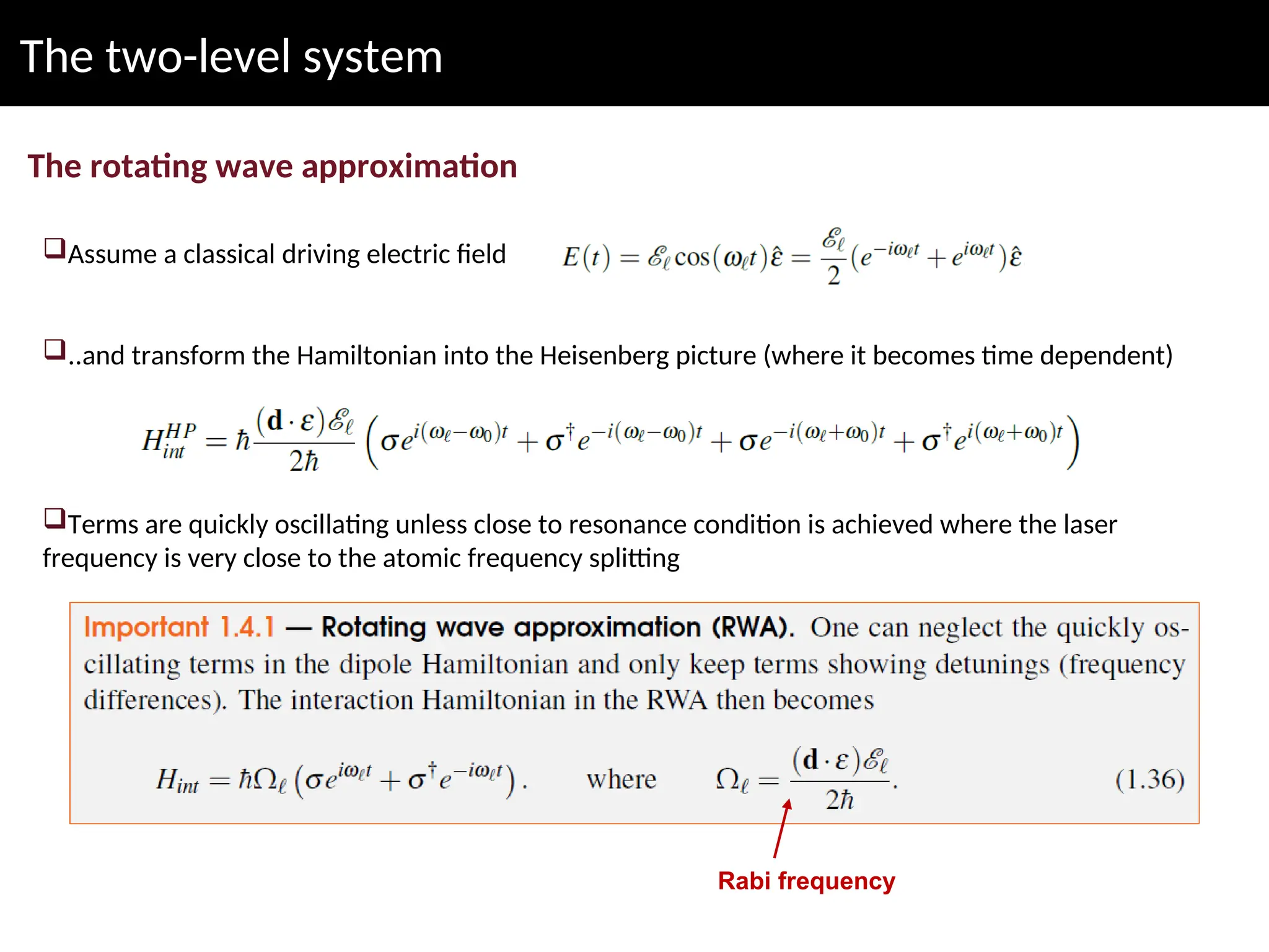
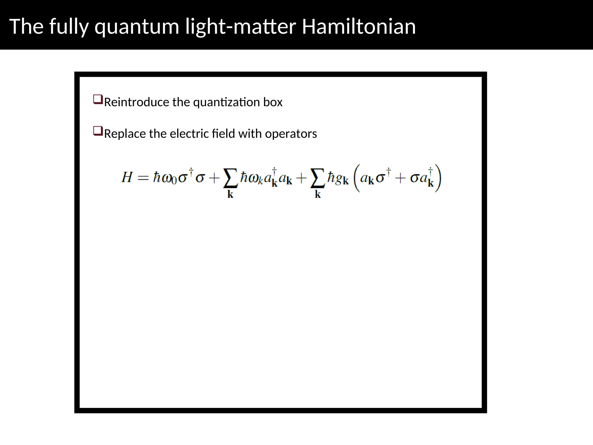
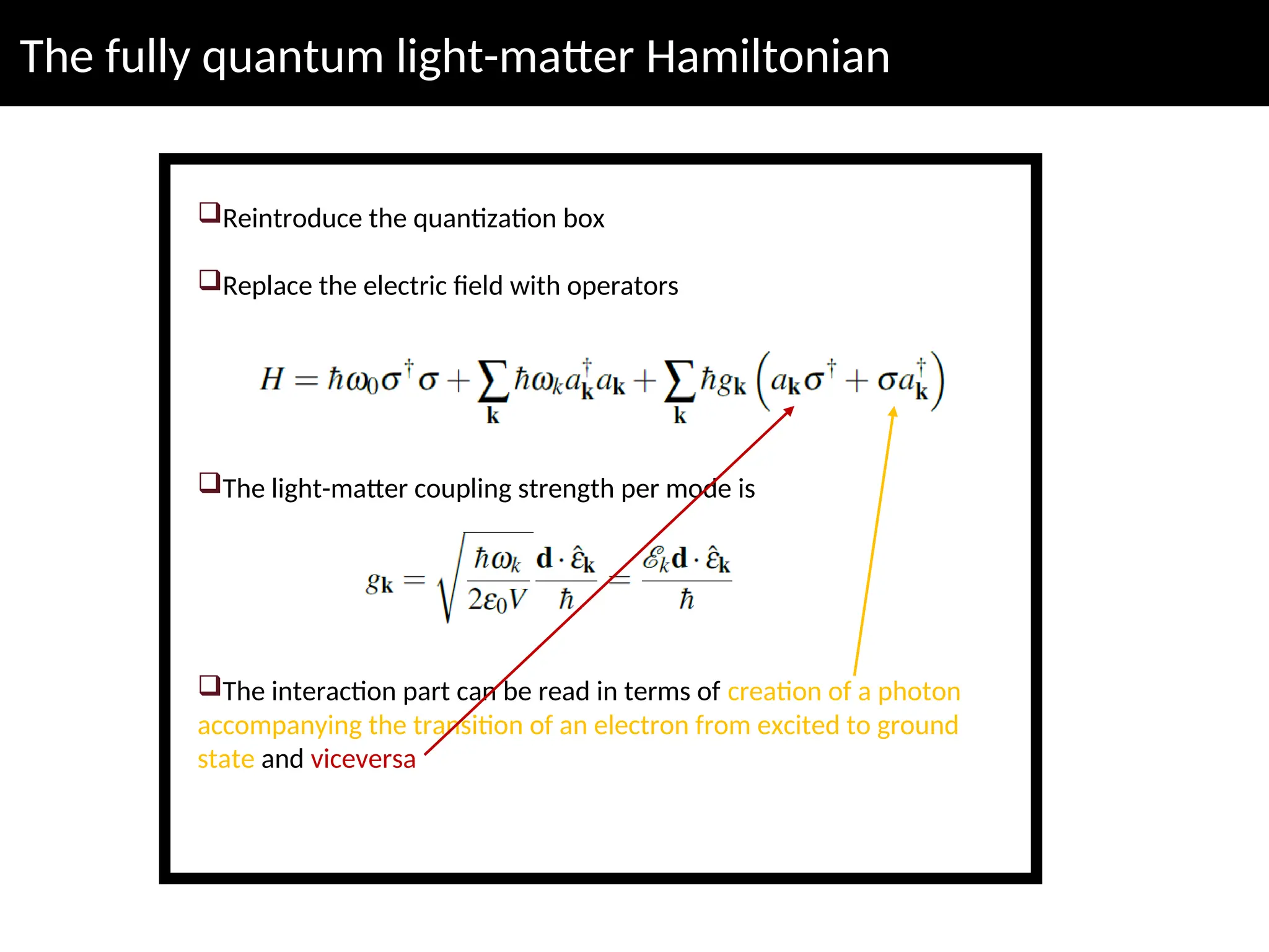
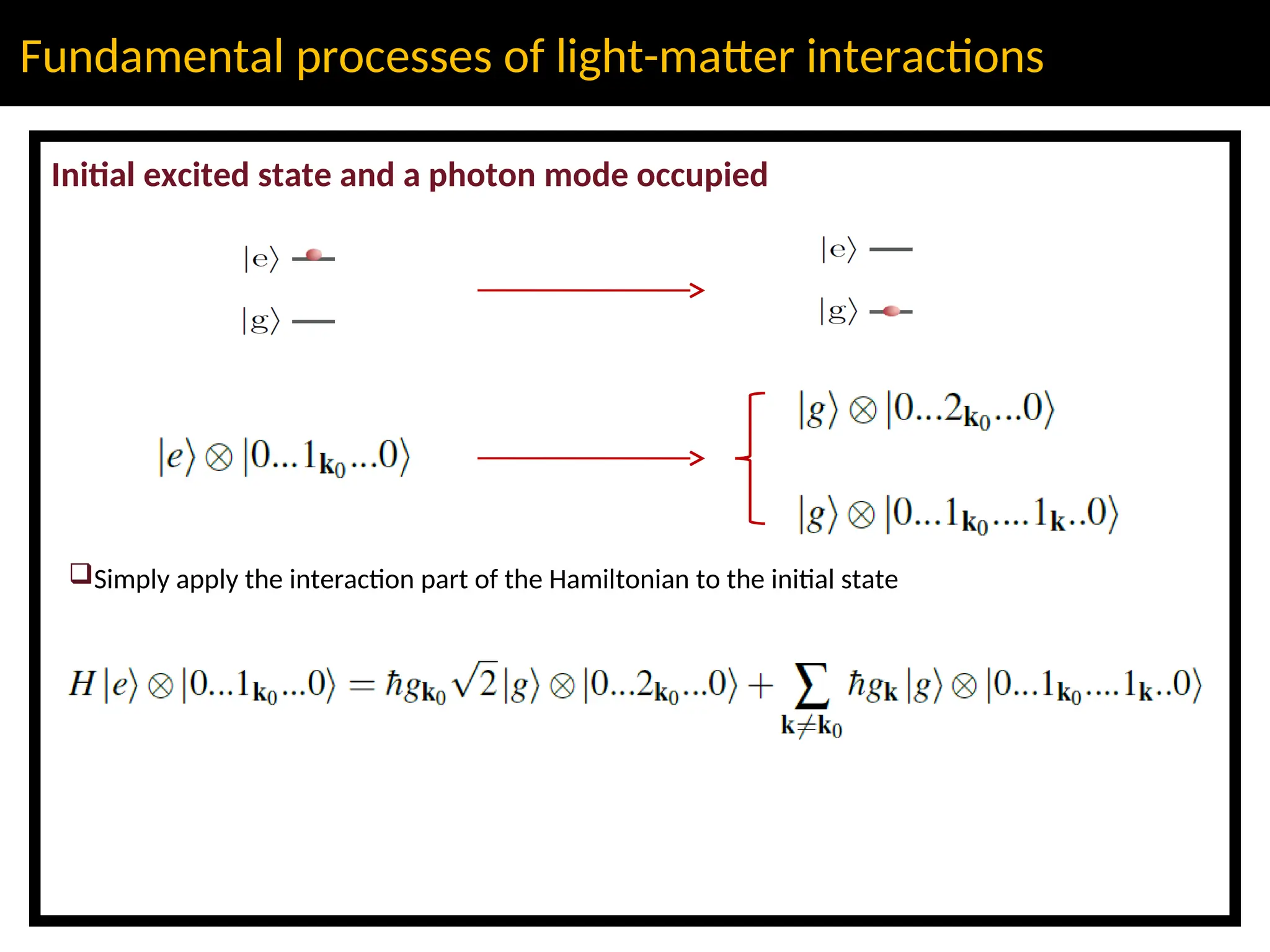
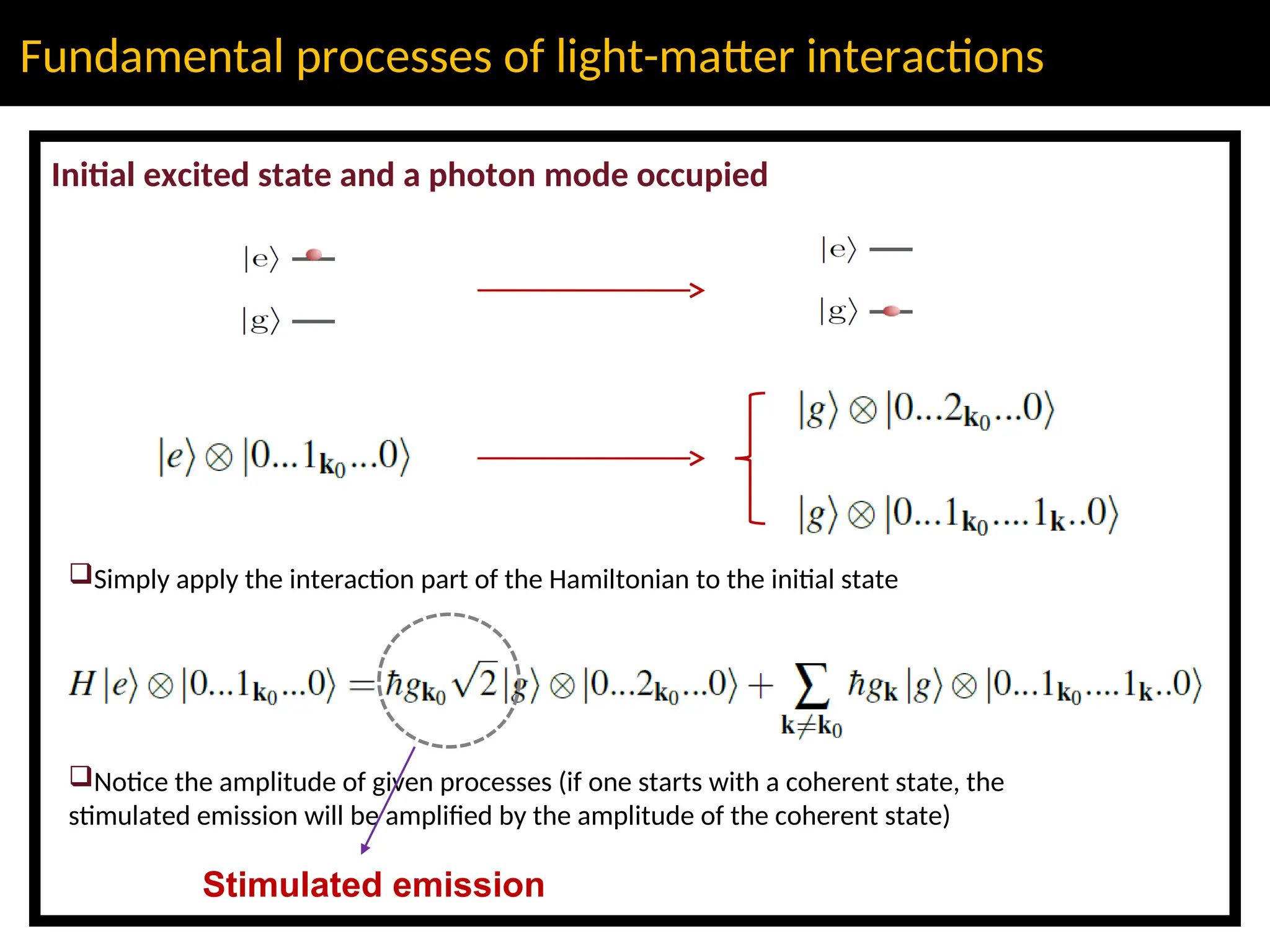
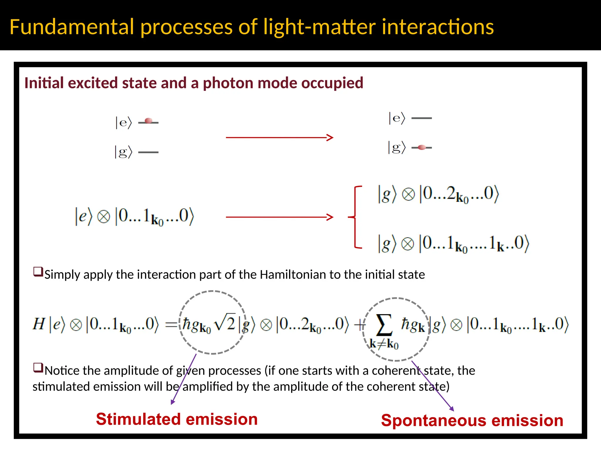
-- Lecture 2 --
Genes Research Group
Cooperative Quantum Phenomena
Quantum Physics of Light-Matter
Interactions
Lecturer: Claudiu Genes
Max Planck Institute for the Science of Light (Erlangen, Germany)
Topics covered in this lecture
Lecture 2
Quantization of the free electromagnetic field
Quantum states of light: number (Fock) basis, coherent states, thermal states
The minimal coupling Hamiltonian: the dipole approximation
The two-level system approximation
The simplified light-matter interaction in the two-level system approximation
Fundamental processes: stimulated absorption/emission and spontaneous emission
Preview of next class: derivation of an open system master equation in the case of spontaneous
emission
Quantization of the free
electromagnetic field in a
fictitiuous box
The quantized electromagnetic field
Take a fictitiuous box of dimensions L x L x L=V
Quantization box
The box is used to simulate an infinite (when L is taken to infinity)
space
No charges or currents present
Boundary conditions (periodic) on the walls of the box
The quantized electromagnetic field
Maxwell’s equations
The quantized electromagnetic field
Maxwell’s equations
Vector and scalar potentials
The quantized electromagnetic field
Maxwell’s equations
Vector and scalar potentials
They are not unique so that one has gauge freedom
A gauge transformation involves adding a scalar field to the problem
such that
The transformed potentials are
..here one can use some useful formulas (from Jackson)
The quantized electromagnetic field
Coulomb gauge
This is obtained by picking a scalar field such that
The quantized electromagnetic field
Coulomb gauge
This is obtained by picking a scalar field such that
From Maxwell’s equations we have which implies
that the scalar potential in the Coulomb gauge is constant and can be
factored out
The quantized electromagnetic field
Coulomb gauge
This is obtained by picking a scalar field such that
From Maxwell’s equations we have which implies
that the scalar potential in the Coulomb gauge is constant and can be
factored out
The wave equation
Solutions can be separated into positive and negative frequency
components
The quantized electromagnetic field
Solving the spatial part
Solutions are of the form of plane waves
The quantized electromagnetic field
Solving the spatial part
Solutions are of the form of plane waves
The normalization makes the solutions orthonormal
The index refers to a direction and amplitude of the allowed
wavevectors and to one of the two transverse polarizations
k-propagation direction
2 possible polarizations
The quantized electromagnetic field
Solving the spatial part
Solutions are of the form of plane waves
From assuming PBC (periodic boundary conditions) we find the set
of allowed wavevectors where the indexes range
from minus to plus infinite integers
The quantized electromagnetic field
Solving the spatial part
Solutions are of the form of plane waves
From assuming PBC (periodic boundary conditions) we find the set
of allowed wavevectors where the indexes range
from minus to plus infinite integers
The resulting expansion of the vector potential into plane waves
And the corresponding electric field
The quantized electromagnetic field
Quantization
Replace c-numbers with non-commuting bosonic operators
The quantized electromagnetic field
Quantization
Replace c-numbers with non-commuting bosonic operators
The electric field operator
Where the zero-point electric field amplitude is
The quantized electromagnetic field
Quantization
Replace c-numbers with non-commuting bosonic operators
The electric field operator
Where the zero-point electric field amplitude is
One can compute
…showing that the total free field Hamiltonian is a sum over an
infinite number of modes each characterized by a quantum harmonic
oscillator operator
The quantized electromagnetic field
A few aspects
The sum over the constant ground state energy diverges in the
infinite volume limit – this gives rise to the Casimir-Polder force (for
more details see https://en.wikipedia.org/wiki/Casimir_effect). We
will disregard this term in the following as it plays no role in the
physics described in this course.
In the Heisenberg picture the operators acquire time dependence
…so that the electric field operator expectation value can be
computed from the initial state vector
The quantized electromagnetic field
Quantum states of light
The number (Fock) basis
The quantized electromagnetic field
Quantum states of light
The number (Fock) basis
How to construct the basis (for an specific mode)
The quantized electromagnetic field
Quantum states of light
Thermal light
*Covered in Exercises 1&2
The quantized electromagnetic field
Quantum states of light
Thermal light
Coherent states
*Covered in Exercises 1&2
The minimal coupling
Hamiltonian: performing the
dipole approximation
Light-matter Hamiltonian in the dipole approximation
The minimal coupling Hamiltonian
Coulomb gauge
Light-matter Hamiltonian in the dipole approximation
The minimal coupling Hamiltonian
Coulomb gauge
Eigenstates in the absence of the external field (a few examples of orbitals below)
Dimension of orbitals (at the level of Å)
Light-matter Hamiltonian in the dipole approximation
The minimal coupling Hamiltonian
Coulomb gauge
Eigenstates in the absence of the external field (a few examples of orbitals below)
Dimension of orbitals (at the level of Å)
Energy difference between orbitals corresponds to wavelengths of few hundred nm
!! The dipole approximation !!
Light-matter Hamiltonian in the dipole approximation
The transformation to the length gauge
Light-matter Hamiltonian in the dipole approximation
The transformation to the length gauge
Length gauge
Light-matter Hamiltonian in the dipole approximation
The transformation to the length gauge
Length gauge
…leads to
Light-matter Hamiltonian in the dipole approximation
The transformation to the length gauge
Length gauge
…leads to
And finally the simplified interaction Hamiltonian
…where the dipole moment is
The two level system (TLS)
approximation
The two-level system
The dipole operator
Only two levels coupled to the external fields
The two-level system
The dipole operator
Only two levels coupled to the external fields
Define ladder operators
…with action
The two-level system
The dipole operator
Only two levels coupled to the external fields
Define ladder operators
…with action
Notice that there is no transition dipole moment within the same orbital (use specific wavefunctions
for Hydrogen atom to check this)
The two-level system
The dipole operator
Only two levels coupled to the external fields
Define ladder operators
…with action
Notice that there is no transition dipole moment within the same orbital (use specific wavefunctions
for Hydrogen atom to check this)
Write the dipole moment operator in the full 2x2 basis
The two-level system
The full Hamiltonian
The free Hamiltonian
…based on the completeness of the basis
The two-level system
The full Hamiltonian
The free Hamiltonian
…based on the completeness of the basis
A couple of simplifications and substract the constant energy term
We then have the full Hamiltonian
The two-level system
The full Hamiltonian
The free Hamiltonian
…based on the completeness of the basis
A couple of simplifications and substract the constant energy term
We then have the full Hamiltonian
…not yet done with approximations!
The two-level system
The rotating wave approximation
Assume a classical driving electric field
..and transform the Hamiltonian into the Heisenberg picture (where it becomes time dependent)
The two-level system
The rotating wave approximation
Assume a classical driving electric field
..and transform the Hamiltonian into the Heisenberg picture (where it becomes time dependent)
Terms are quickly oscillating unless close to resonance condition is achieved where the laser
frequency is very close to the atomic frequency splitting
Rabi frequency
The fully quantum light-
matter Hamiltonian
The fully quantum light-matter Hamiltonian
Reintroduce the quantization box
Replace the electric field with operators
The fully quantum light-matter Hamiltonian
Reintroduce the quantization box
Replace the electric field with operators
The light-matter coupling strength per mode is
The interaction part can be read in terms of creation of a photon
accompanying the transition of an electron from excited to ground
state and viceversa
Fundamental processes:
stimulated
absorption/emission and
spontaneous emission
Fundamental processes of light-matter interactions
Initial excited state and a photon mode occupied
Fundamental processes of light-matter interactions
Initial excited state and a photon mode occupied
Simply apply the interaction part of the Hamiltonian to the initial state
Fundamental processes of light-matter interactions
Initial excited state and a photon mode occupied
Simply apply the interaction part of the Hamiltonian to the initial state
Notice the amplitude of given processes (if one starts with a coherent state, the
stimulated emission will be amplified by the amplitude of the coherent state)
Stimulated emission
Fundamental processes of light-matter interactions
Initial excited state and a photon mode occupied
Simply apply the interaction part of the Hamiltonian to the initial state
Notice the amplitude of given processes (if one starts with a coherent state, the
stimulated emission will be amplified by the amplitude of the coherent state)
Stimulated emission Spontaneous emission
Fundamental processes of light-matter interactions
Initial ground state and a photon mode occupied
Fundamental processes of light-matter interactions
Initial ground state and a photon mode occupied
Simply apply the interaction part of the Hamiltonian to the initial state
Fundamental processes of light-matter interactions
Initial ground state and a photon mode occupied
Simply apply the interaction part of the Hamiltonian to the initial state
The same argument as before applies here as well (if one starts with a coherent state,
the stimulated absorption will be amplified by the amplitude of the coherent state)
Stimulated absorption
Preview of Lecture 3
Open system dynamics - dissipation
The need for a master equation
Dynamics in the quantization box is complicated to describe: owing to the infinite
dimensional Hilbert space
One would desire to reduce the dynamics to the system of interest (the two level
system – a two dimensional Hilbert space)
Open system dynamics - dissipation
The need for a master equation
Dynamics in the quantization box is complicated to describe: owing to the infinite
dimensional Hilbert space
One would desire to reduce the dynamics to the system of interest (the two level
system – a two dimensional Hilbert space)
First step: dynamics can be followed at the level of the density operator (von-Neumann
equation of motion)
Some factorization assumption can be employed
Open system dynamics - dissipation
The procedure…
Perform a formal integration (exact, there are no approximations)
Another formal time integration (still exact)
Open system dynamics - dissipation
The procedure…
Perform a formal integration (exact, there are no approximations)
Another formal time integration (still exact)
Open system dynamics - dissipation
The procedure…
Perform a formal integration (exact, there are no approximations)
Another formal time integration (still exact)
Keep doing this for a sequence of ordered times
Open system dynamics - dissipation
The procedure…
Perform a formal integration (exact, there are no approximations)
Another formal time integration (still exact)
Keep doing this for a sequence of ordered times
Truncate (this is where the approximation comes in)
Open system dynamics - dissipation
The important step…
Trace over the field states (equivalent to eliminating the box)
Next steps in the following lecture…

QPLMI21_-_Lecture_2.ppt quantum physic f

  • 1.
    -- Lecture 2-- Genes Research Group Cooperative Quantum Phenomena Quantum Physics of Light-Matter Interactions Lecturer: Claudiu Genes Max Planck Institute for the Science of Light (Erlangen, Germany)
  • 2.
    Topics covered inthis lecture Lecture 2 Quantization of the free electromagnetic field Quantum states of light: number (Fock) basis, coherent states, thermal states The minimal coupling Hamiltonian: the dipole approximation The two-level system approximation The simplified light-matter interaction in the two-level system approximation Fundamental processes: stimulated absorption/emission and spontaneous emission Preview of next class: derivation of an open system master equation in the case of spontaneous emission
  • 3.
    Quantization of thefree electromagnetic field in a fictitiuous box
  • 4.
    The quantized electromagneticfield Take a fictitiuous box of dimensions L x L x L=V Quantization box The box is used to simulate an infinite (when L is taken to infinity) space No charges or currents present Boundary conditions (periodic) on the walls of the box
  • 5.
    The quantized electromagneticfield Maxwell’s equations
  • 6.
    The quantized electromagneticfield Maxwell’s equations Vector and scalar potentials
  • 7.
    The quantized electromagneticfield Maxwell’s equations Vector and scalar potentials They are not unique so that one has gauge freedom A gauge transformation involves adding a scalar field to the problem such that The transformed potentials are
  • 8.
    ..here one canuse some useful formulas (from Jackson)
  • 9.
    The quantized electromagneticfield Coulomb gauge This is obtained by picking a scalar field such that
  • 10.
    The quantized electromagneticfield Coulomb gauge This is obtained by picking a scalar field such that From Maxwell’s equations we have which implies that the scalar potential in the Coulomb gauge is constant and can be factored out
  • 11.
    The quantized electromagneticfield Coulomb gauge This is obtained by picking a scalar field such that From Maxwell’s equations we have which implies that the scalar potential in the Coulomb gauge is constant and can be factored out The wave equation Solutions can be separated into positive and negative frequency components
  • 12.
    The quantized electromagneticfield Solving the spatial part Solutions are of the form of plane waves
  • 13.
    The quantized electromagneticfield Solving the spatial part Solutions are of the form of plane waves The normalization makes the solutions orthonormal The index refers to a direction and amplitude of the allowed wavevectors and to one of the two transverse polarizations k-propagation direction 2 possible polarizations
  • 14.
    The quantized electromagneticfield Solving the spatial part Solutions are of the form of plane waves From assuming PBC (periodic boundary conditions) we find the set of allowed wavevectors where the indexes range from minus to plus infinite integers
  • 15.
    The quantized electromagneticfield Solving the spatial part Solutions are of the form of plane waves From assuming PBC (periodic boundary conditions) we find the set of allowed wavevectors where the indexes range from minus to plus infinite integers The resulting expansion of the vector potential into plane waves
  • 16.
    The quantized electromagneticfield Solving the spatial part Solutions are of the form of plane waves From assuming PBC (periodic boundary conditions) we find the set of allowed wavevectors where the indexes range from minus to plus infinite integers The resulting expansion of the vector potential into plane waves And the corresponding electric field
  • 17.
    The quantized electromagneticfield Quantization Replace c-numbers with non-commuting bosonic operators
  • 18.
    The quantized electromagneticfield Quantization Replace c-numbers with non-commuting bosonic operators The electric field operator Where the zero-point electric field amplitude is
  • 19.
    The quantized electromagneticfield Quantization Replace c-numbers with non-commuting bosonic operators The electric field operator Where the zero-point electric field amplitude is One can compute …showing that the total free field Hamiltonian is a sum over an infinite number of modes each characterized by a quantum harmonic oscillator operator
  • 20.
    The quantized electromagneticfield A few aspects The sum over the constant ground state energy diverges in the infinite volume limit – this gives rise to the Casimir-Polder force (for more details see https://en.wikipedia.org/wiki/Casimir_effect). We will disregard this term in the following as it plays no role in the physics described in this course.
  • 21.
    The quantized electromagneticfield A few aspects The sum over the constant ground state energy diverges in the infinite volume limit – this gives rise to the Casimir-Polder force (for more details see https://en.wikipedia.org/wiki/Casimir_effect). We will disregard this term in the following as it plays no role in the physics described in this course. In the Heisenberg picture the operators acquire time dependence
  • 22.
    The quantized electromagneticfield A few aspects The sum over the constant ground state energy diverges in the infinite volume limit – this gives rise to the Casimir-Polder force (for more details see https://en.wikipedia.org/wiki/Casimir_effect). We will disregard this term in the following as it plays no role in the physics described in this course. In the Heisenberg picture the operators acquire time dependence …so that the electric field operator expectation value can be computed from the initial state vector
  • 23.
    The quantized electromagneticfield Quantum states of light The number (Fock) basis
  • 24.
    The quantized electromagneticfield Quantum states of light The number (Fock) basis How to construct the basis (for an specific mode)
  • 25.
    The quantized electromagneticfield Quantum states of light Thermal light *Covered in Exercises 1&2
  • 26.
    The quantized electromagneticfield Quantum states of light Thermal light Coherent states *Covered in Exercises 1&2
  • 27.
    The minimal coupling Hamiltonian:performing the dipole approximation
  • 28.
    Light-matter Hamiltonian inthe dipole approximation The minimal coupling Hamiltonian Coulomb gauge
  • 29.
    Light-matter Hamiltonian inthe dipole approximation The minimal coupling Hamiltonian Coulomb gauge Eigenstates in the absence of the external field (a few examples of orbitals below) Dimension of orbitals (at the level of Å)
  • 30.
    Light-matter Hamiltonian inthe dipole approximation The minimal coupling Hamiltonian Coulomb gauge Eigenstates in the absence of the external field (a few examples of orbitals below) Dimension of orbitals (at the level of Å) Energy difference between orbitals corresponds to wavelengths of few hundred nm
  • 31.
    Light-matter Hamiltonian inthe dipole approximation The minimal coupling Hamiltonian Coulomb gauge Eigenstates in the absence of the external field (a few examples of orbitals below) Dimension of orbitals (at the level of Å) Energy difference between orbitals corresponds to wavelengths of few hundred nm !! The dipole approximation !!
  • 32.
    Light-matter Hamiltonian inthe dipole approximation The transformation to the length gauge
  • 33.
    Light-matter Hamiltonian inthe dipole approximation The transformation to the length gauge Length gauge
  • 34.
    Light-matter Hamiltonian inthe dipole approximation The transformation to the length gauge Length gauge …leads to
  • 35.
    Light-matter Hamiltonian inthe dipole approximation The transformation to the length gauge Length gauge …leads to And finally the simplified interaction Hamiltonian …where the dipole moment is
  • 36.
    The two levelsystem (TLS) approximation
  • 37.
    The two-level system Thedipole operator Only two levels coupled to the external fields
  • 38.
    The two-level system Thedipole operator Only two levels coupled to the external fields Define ladder operators …with action
  • 39.
    The two-level system Thedipole operator Only two levels coupled to the external fields Define ladder operators …with action Notice that there is no transition dipole moment within the same orbital (use specific wavefunctions for Hydrogen atom to check this)
  • 40.
    The two-level system Thedipole operator Only two levels coupled to the external fields Define ladder operators …with action Notice that there is no transition dipole moment within the same orbital (use specific wavefunctions for Hydrogen atom to check this) Write the dipole moment operator in the full 2x2 basis
  • 41.
    The two-level system Thefull Hamiltonian The free Hamiltonian …based on the completeness of the basis
  • 42.
    The two-level system Thefull Hamiltonian The free Hamiltonian …based on the completeness of the basis A couple of simplifications and substract the constant energy term We then have the full Hamiltonian
  • 43.
    The two-level system Thefull Hamiltonian The free Hamiltonian …based on the completeness of the basis A couple of simplifications and substract the constant energy term We then have the full Hamiltonian …not yet done with approximations!
  • 44.
    The two-level system Therotating wave approximation Assume a classical driving electric field ..and transform the Hamiltonian into the Heisenberg picture (where it becomes time dependent)
  • 45.
    The two-level system Therotating wave approximation Assume a classical driving electric field ..and transform the Hamiltonian into the Heisenberg picture (where it becomes time dependent) Terms are quickly oscillating unless close to resonance condition is achieved where the laser frequency is very close to the atomic frequency splitting Rabi frequency
  • 46.
    The fully quantumlight- matter Hamiltonian
  • 47.
    The fully quantumlight-matter Hamiltonian Reintroduce the quantization box Replace the electric field with operators
  • 48.
    The fully quantumlight-matter Hamiltonian Reintroduce the quantization box Replace the electric field with operators The light-matter coupling strength per mode is The interaction part can be read in terms of creation of a photon accompanying the transition of an electron from excited to ground state and viceversa
  • 49.
  • 50.
    Fundamental processes oflight-matter interactions Initial excited state and a photon mode occupied
  • 51.
    Fundamental processes oflight-matter interactions Initial excited state and a photon mode occupied Simply apply the interaction part of the Hamiltonian to the initial state
  • 52.
    Fundamental processes oflight-matter interactions Initial excited state and a photon mode occupied Simply apply the interaction part of the Hamiltonian to the initial state Notice the amplitude of given processes (if one starts with a coherent state, the stimulated emission will be amplified by the amplitude of the coherent state) Stimulated emission
  • 53.
    Fundamental processes oflight-matter interactions Initial excited state and a photon mode occupied Simply apply the interaction part of the Hamiltonian to the initial state Notice the amplitude of given processes (if one starts with a coherent state, the stimulated emission will be amplified by the amplitude of the coherent state) Stimulated emission Spontaneous emission
  • 54.
    Fundamental processes oflight-matter interactions Initial ground state and a photon mode occupied
  • 55.
    Fundamental processes oflight-matter interactions Initial ground state and a photon mode occupied Simply apply the interaction part of the Hamiltonian to the initial state
  • 56.
    Fundamental processes oflight-matter interactions Initial ground state and a photon mode occupied Simply apply the interaction part of the Hamiltonian to the initial state The same argument as before applies here as well (if one starts with a coherent state, the stimulated absorption will be amplified by the amplitude of the coherent state) Stimulated absorption
  • 57.
  • 58.
    Open system dynamics- dissipation The need for a master equation Dynamics in the quantization box is complicated to describe: owing to the infinite dimensional Hilbert space One would desire to reduce the dynamics to the system of interest (the two level system – a two dimensional Hilbert space)
  • 59.
    Open system dynamics- dissipation The need for a master equation Dynamics in the quantization box is complicated to describe: owing to the infinite dimensional Hilbert space One would desire to reduce the dynamics to the system of interest (the two level system – a two dimensional Hilbert space) First step: dynamics can be followed at the level of the density operator (von-Neumann equation of motion)
  • 60.
    Open system dynamics- dissipation The need for a master equation Dynamics in the quantization box is complicated to describe: owing to the infinite dimensional Hilbert space One would desire to reduce the dynamics to the system of interest (the two level system – a two dimensional Hilbert space) First step: dynamics can be followed at the level of the density operator (von-Neumann equation of motion) Some factorization assumption can be employed
  • 61.
    Open system dynamics- dissipation The procedure… Perform a formal integration (exact, there are no approximations) Another formal time integration (still exact)
  • 62.
    Open system dynamics- dissipation The procedure… Perform a formal integration (exact, there are no approximations) Another formal time integration (still exact)
  • 63.
    Open system dynamics- dissipation The procedure… Perform a formal integration (exact, there are no approximations) Another formal time integration (still exact) Keep doing this for a sequence of ordered times
  • 64.
    Open system dynamics- dissipation The procedure… Perform a formal integration (exact, there are no approximations) Another formal time integration (still exact) Keep doing this for a sequence of ordered times Truncate (this is where the approximation comes in)
  • 65.
    Open system dynamics- dissipation The important step… Trace over the field states (equivalent to eliminating the box) Next steps in the following lecture…