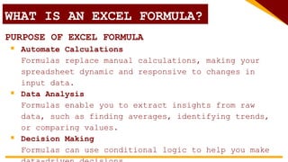
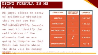
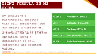
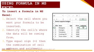
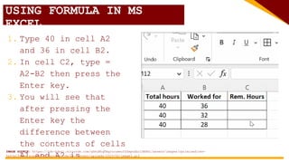
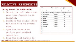
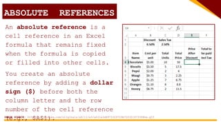
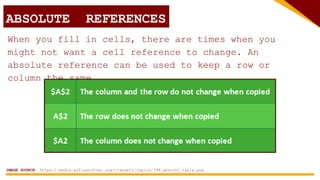
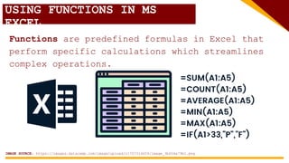
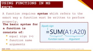
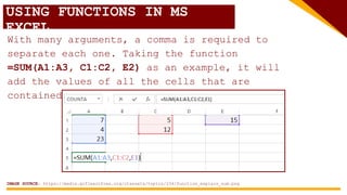
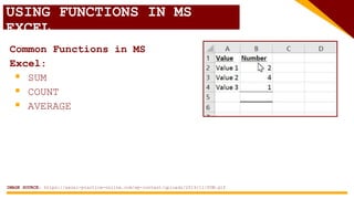
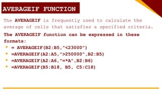
QMMS Lesson 2 - Using Excel Formula.pptx

POLYTECHNIC UNIVERSITY OF THE PHILIPPINES - BIÑAN
COLLEGE OF INFORMATION TECHNOLOGY AND ENGINEERING (CITE)
USING FORMULA
IN MS EXCEL
Lesson 2 – Quantitative Methods with Modelling and Simulation
ROWELL L. MARQUINA
Professional Lecturer

LEARNING OBJECTIVES:
At the end of the session, students will be
able to:
 understand the concept of
formulas in Excel.
 learn the basic syntax for
creating formulas.
 practice using common
functions
 apply formulas to solve real-
world problems or analyze
provided datasets.
IMAGE SOURCE: https://img.freepik.com/premium-vector/flat-isometric-illustration-concept-pile-books-ideas-targets_18660-
2027.jpg

WHAT IS AN EXCEL FORMULA?
An Excel formula is an expression placed within
a cell that performs calculations,
manipulations, or other actions on data in your
spreadsheet.
= A1 + A2 +
A3
= SUM
(A1:A3)

WHAT IS AN EXCEL FORMULA?
PURPOSE OF EXCEL FORMULA
 Automate Calculations
Formulas replace manual calculations, making your
spreadsheet dynamic and responsive to changes in
input data.
 Data Analysis
Formulas enable you to extract insights from raw
data, such as finding averages, identifying trends,
or comparing values.
 Decision Making
Formulas can use conditional logic to help you make

An excel formula is
consists
of the following
components:
 Operators
 Cell References
 Functions
 Constants
COMPONENTS OF EXCEL FORMULA
IMAGE SOURCE: https://cdn.ablebits.com/_img-blog/excel-calculations/excel-calculations.png

Operators refers to symbols
that indicate the
arithmetic operation to be
performed in a formula.
It follows the rule of
PEMDAS in performing its
operation which means that
when writing formula, you
should consider the order of
operations according to the
said rule.
IMAGE SOURCE: https://www.projectcubicle.com/wp-content/uploads/2022/05/excel-formulas-arithmetic-operators-
e1651596319655.webp

Cell References also known
as “cell address” is a
component of the excel
formula that indicates the
location of data within
the spreadsheet.
IMAGE SOURCE: https://media.gcflearnfree.org/ctassets/topics/234/cell_intro_address.png
It is a combination of a
column letter and a row
number that identifies a
cell on a worksheet.

Functions are predefined formulas in Excel that
perform specific calculations which streamlines
complex operations.
IMAGE SOURCE: https://images.datacamp.com/image/upload/v1707314659/image_3b654e79b1.png

USING FORMULA IN MS
EXCEL
MS Excel offers an array
of arithmetic operators
that we can use for
writing formula.
IMAGE SOURCE: https://www.projectcubicle.com/wp-content/uploads/2022/05/excel-formulas-arithmetic-operators-
e1651596319655.webp
To use data in a formula
we need to identify the
cell address of the
elements that we are
going to compute so that
Excel can locate where
the data will be coming
from.

USING FORMULA IN MS
EXCEL
By combining a
mathematical operator
with cell references, you
can create a variety of
simple formulas in Excel.
IMAGE SOURCE: https://media.gcflearnfree.org/ctassets/topics/198/simpform_graphic_formulas5.png
A formula can also perform
operation using a
combination of cell
references and constant
values.

USING FORMULA IN MS
EXCEL
To insert a formula in MS
Excel:
1. Select the cell where you
want your formula to be
inserted.
2. Identify the cell/s where
from.
3. Type equal sign (=) then
the combination of cell
address and arithmetic
IMAGE SOURCE: https://www.guru99.com/images/5-2015/excel_formulas_demo2.gif

USING FORMULA IN MS
EXCEL
1. Type 40 in cell A2
and 36 in cell B2.
2. In cell C2, type =
A2-B2 then press the
Enter key.
3. You will see that
after pressing the
Enter key the
difference between
the contents of cells
A1 and A2 is
IMAGE SOURCE: https://cdn-kdnkj.nitrocdn.com/qYmjBhqTAqJorzweuYZZmpnSbrlDEHHj/assets/images/optimized/rev-
5a63a19/www.academyoflearning.com/wp-content/uploads/2023/02/image3.gif

USING OPERATORS IN MS
EXCEL
1.Type 78 in cell B2 and
235 in cell C2.
2.In cell D2, type =
B2/C2 then press the
Enter key.
3.You will see that
after pressing the
Enter key the result
of dividing the entry
in cell B2 divided by
IMAGE SOURCE: https://insidetheweb.com/wp-content/uploads/2023/05/How-to-Calculate-Percentage-in-Excel.gif

VIDEO SOURCE:
https://www.youtube.co
m/watch?v=xc14gFFyiTw&
t=7s

LET’S PRACTICE!
Consider the image at the
right, write the formula to
compute for the following:
 sum of 1st and 2nd number
 product of 3rd and 4th
number
 the square of the 2nd
number
 difference between 2nd
and 4th number
 sum 1st to 4th number

USING FORMULA IN MS
EXCEL
There will be cases where the formula will require
to use two or more arithmetic operators.
In those cases, you should consider writing
the formula following the order of
operations:
 Operations enclosed in parentheses
 Exponential calculations (3^2, for example)
 Multiplication and division, whichever
comes first
 Addition and subtraction, whichever comes

VIDEO SOURCE:
m/watch?v=J-W3thqtDpQ

LET’S PRACTICE!
Consider the image at the
right, write the formula to
compute for the following:
 product of multiplying
the sum of 1st and 2nd
number by 10
 difference of 3rd and 4th
number divided by the 2nd
number
 cube of 3rd number
multiplied by the 1st

LET’S PRACTICE!
Consider the image below, write
the formula to compute for the
following:
 Semestral Average of every
subject
 Average of 3rd and 4th Quarter
 Semestral Average

RELATIVE
AND ABSOLUTE
REFERENCES

RELATIVE
REFERENCES
Relative references are cell references in formulas
that adjust automatically when you copy or fill the
formula into other cells.
IMAGE SOURCE: https://cdn.educba.com/academy/wp-content/uploads/2019/07/cell-references-in-excel-2.gif

RELATIVE
REFERENCES
They are the default type of reference in Excel and
are essential for replicating calculations or patterns
across multiple cells.
Relativity is based on direction, When you copy a
formula, relative references change based on the
relative position of the original and copied cells.
 Copying down rows: Row numbers in the reference
will increase.
 Copying across columns: Column letters in the
reference will shift.

RELATIVE REFERENCES
Using Relative Reference:
1. Select the cell where you
want your formula to be
inserted.
2. Identify the cell/s where
from.
3. Type the formula to
perform your desired
operation.
4. Drag the fill handle to
over the cells that you
IMAGE SOURCE: https://qph.cf2.quoracdn.net/main-qimg-7c031e451e96b5cc07cfa2bf62261230

ABSOLUTE REFERENCES
An absolute reference is a
cell reference in an Excel
formula that remains fixed
when the formula is copied
or filled into other cells.
IMAGE SOURCE: https://i.pinimg.com/originals/a0/11/e3/a011e3d4973329729b7203214733086a.gif
You create an absolute
reference by adding a dollar
sign ($) before both the
column letter and the row
number of the cell reference
(e.g., $A$1).

ABSOLUTE REFERENCES
When you fill in cells, there are times when you
might not want a cell reference to change. An
absolute reference can be used to keep a row or
column the same.
IMAGE SOURCE: https://media.gcflearnfree.org/ctassets/topics/198/absorel_table.png

VIDEO SOURCE:
m/watch?v=iDg9s7BJ2m4

USING FUNCTIONS IN MS
EXCEL
Functions are predefined formulas in Excel that
perform specific calculations which streamlines
complex operations.
IMAGE SOURCE: https://images.datacamp.com/image/upload/v1707314659/image_3b654e79b1.png

EXCEL
A function requires syntax which refers to the
exact way a function must be written to perform
properly.
IMAGE SOURCE: https://media.gcflearnfree.org/content/563b7aa7ca7fac0d9c7b3f7a_11_05_2015/functions_syntax_graphic.png
The basic syntax for
a function is
consists of:
 equal sign (=)
 function name
 arguments

EXCEL
With many arguments, a comma is required to
separate each one. Taking the function
=SUM(A1:A3, C1:C2, E2) as an example, it will
add the values of all the cells that are
contained within the three arguments.
IMAGE SOURCE: https://media.gcflearnfree.org/ctassets/topics/234/function_explain_sum.png

EXCEL
Common Functions in MS
Excel:
 SUM
 COUNT
 AVERAGE
IMAGE SOURCE: https://excel-practice-online.com/wp-content/uploads/2019/11/SUM.gif

SUM FUNCTION
The SUM function adds values from
individual cells, cell ranges, multiple
cell ranges or its combination.
The SUM function can be expressed in these
formats:
 = SUM (A2, B4, C3)
computes sum for individual cells
 = SUM (A1:A10)
computes sum for a range
 = SUM (A1:A5, B1:B5, C1:C5)
computes sum for multiple ranges

SUMIF FUNCTION
The SUMIF function is
used to compute for the
sum of numbers inside a
specified range that
satisfies specific
conditions.
The formula for range should be expressed in
this format
= SUMIF(criteria_range, criteria,
sum_range)
IMAGE SOURCE: https://excel-practice-online.com/wp-content/uploads/2019/11/SUMIF.gif

SUMIF FUNCTION
Consider a scenario
where you have a
dataset containing
product and quantities
sold. You are tasked
by your manager to
create a table that
will present the total
number of fruits sold.

SUMIF FUNCTION
The first thing we need to
find is the sum_range. The
sum_range contains the
numerical values that are
necessary for the computation.
From this table, you can see
that Column B, or the
quantities sold contains the
values that are required to
be computed for total. We can
identify Column B, (B2:B7),
as our sum_range.

SUMIF FUNCTION
After successfully
identifying the
sum_range, let us now
identify what is the
criteria and the
criteria_range. The
criteria is the basis or
reference of your
search.
The criteria_range
refers to the range of
cells that contains
the criteria.

SUMIF FUNCTION
From this table, since we
are looking for total
number of each fruit sold,
we identify the fruits
“Apples”, “Watermelons”,
and “Bananas” as criteria.
The range that contains
the criteria is considered
as criteria_range which in
this case is Column A,
A2:A7.

SUMIF FUNCTION
Now that we know the
sum_range (B1:B7), criteria
(name of fruit), and
criteria_range (A1:A7), we
can now write our formula.
Using the format:
= SUMIF(criteria_range,
criteria, sum_range) find a
cell where you want the
total number of apples sold
to appear and type:
=SUMIF(A1:A7, “APPLES”,

SUMIF FUNCTION
Alternatively, you can also
use:
=SUMIF(A1:A7, A2, B1:B7)
where A2 is the cell the
word “Apples”.
Fortunately, the first
letter of each fruit is
different from each other
that is why we can make use
of a wild card or (*).
=SUMIF(A1:A7, “A*”, B1:B7)
where “A*” means to compute
for anything that starts

SUMIFS FUNCTION
The SUMIFS function,
one of the Excel
functions that adds
all the numbers that
meet multiple
criteria.
=SUMIFS(A2:A17, B2:B17, "B*“ , C2:C17, “T*)
=SUMIFS(A2:A17,B2:B17,"=BANANAS",C2:C17,"=Tom")
IMAGE SOURCE: https://excel-practice-online.com/wp-content/uploads/2019/11/sumifs.gif

SUMIFS FUNCTION
Consider a scenario where you have a dataset
containing product, quantities sold and names of
salespersons. You are tasked to create a table
that will present the total number of fruits
sold by Tom. From this table, you can see
that Column B, or the
quantities sold contains the
values that are required to
be computed for total. The
range in column B, (B2:B7),
is determined as the

SUMIFS FUNCTION
After successfully identifying
the sum_range, let us now
identify what is the criteria1
and the criteria_range1 since
there are two criteria needed
for this context.
From this table, since we are looking for total number
of each fruit sold as first criteria 1, we identify the
fruits “Apples”, “Watermelons”, and “Bananas” as
criteria1.
The range in column that contains the criteria1 is
considered as criteria_range1 which in this case is A2:A7.

SUMIFS FUNCTION
After s identifying the
criteria1, let us now
identify what is the
criteria2 and the
criteria_range2 since there
are two criteria needed for
this context.
From this table, since we are looking for total number
of each fruit sold by the salesperson as second
criteria 1, we identify the “Tom” and “Sarah” as
criteria2.
The range in column that contains the criteria2 is
considered as criteria_range2 which in this case is C2:C7.

SUMIFS FUNCTION
Now that we have all the elements, we can
use the formula below to get the total
number of apples sold by Tom:
Using the format:
= SUMIFS(sum_range, criteria_range1, criteria1,
criteria_range2, criteria2) find a cell where
you want the total number of apples sold by Tom
to appear and type:
=SUMIFS(A1:A7, B1:B7,“APPLES”, C1:C7,”TOM”)

VIDEO SOURCE:
m/watch?v=dI8w0utjUc0

COUNT FUNCTION
The COUNT function calculates the total number of
cells that contain numerical values, including
numbers found inside the given list of inputs.
The COUNT function can be expressed in these formats:
 = COUNT (A1, A7, A15) computes total for specific
cells
 = COUNT (A1:A50 ) computes total for ranges
 = COUNT (A1:A5, B1:B5) computes total for multiple
For example, if the range A1:A20 contains the values
to be counted, the formula =COUNT(A1:A20) returns the
total numbers of that range.

COUNTIF FUNCTION
The COUNTIF function is
used to count numbers
of values within a
specified range that
satisfies specific
criteria.
The formula for range should be expressed in
this format
= COUNTIF(criteria_range, criteria)
= COUNTIF(B2:B25,">5)
IMAGE SOURCE: https://excel-practice-online.com/wp-content/uploads/2019/11/COUNTIF.gif

Consider a scenario
where you have a
dataset containing
names. You are tasked
by your manager to
count the number of
times a particular
name appeared in the
table.
COUNTIF FUNCTION

From the syntax:
=COUNTIF(criteria_range,
criteria)
We can use the formula:
=COUNTIF(A2:A10, “Charmaine”)
The formula above will
compute for the number of
times the name “Charmaine”
appeared in the table.
COUNTIF FUNCTION

Alternatively, we can use:
 =COUNTIF(A2:A10, A3)
we can use cell A3 as reference
point since it contains the
value “Charmaine”.
 =COUNTIF(A2:A10, “C*”)
we can also make use of the
wild card “C*” since the name
Charmaine is the only value in
the table that starts with
letter “C”.
COUNTIF FUNCTION

The COUNTIFS function is function in Excel that
tallies the number of cells within a specified
range that meet one or more specified conditions.
COUNTIFS FUNCTION
The conditions are referred to as critera1,
criteria2, .. and so on, which can check things
like:
 If a number is greater than another number >
 If a number is smaller than another number <
 If a number or text is equal to something =
 If a number or text is greater than equal to
something >=

From this table, we want
to know the number of
students who earned an
average of 90 and but
less than 95.
Since we are looking
for average the
criteria range is
Column B, B2:B10.
COUNTIF FUNCTION
COUNTIFS FUNCTION

To count the cells that
contain grades with average of
90 and but less than 95, we
need to employ two criteria:
 grade that is greater than
or equal to 90 (>=90)
 grade that is less than 95
(<95)
COUNTIF FUNCTION
COUNTIFS FUNCTION

Using the syntax for COUNTIFS:
=COUNTIFS(criteria_range1, criteria, criteria_range2,
criteria2)
We can arrive with the formula:
=COUNTIFS(B2:B10,”>=90”, B2:B10, “<95”)
COUNTIF FUNCTION
COUNTIFS FUNCTION
We use B2:B10 as criteria_range1 and criteria_range2
because it is the only column that contains our
criteria.

VIDEO SOURCE:
m/watch?v=OFqQqdr9R44

AVERAGE FUNCTION
The AVERAGE function returns the average (arithmetic
mean) of the arguments.
The AVERAGE function can be expressed in these
formats:
 = AVERAGE (A1, A7, A15) computes average for
specific cells
 = AVERAGE (A1:A50 ) computes average for ranges
 = AVERAGE (A1:A5, B1:B5) computes ave for multiple
ranges
For example, if the range A1:A20 contains numbers,
the formula =AVERAGE(A1:A20) returns the average of
those numbers.

AVERAGEIF FUNCTION
The AVERAGEIF is frequently used to calculate the
average of cells that satisfies a specified criteria.
The AVERAGEIF function can be expressed in these
formats:
 = AVERAGEIF(B2:B5,"<23000")
 =AVERAGEIF(A2:A5,">250000",B2:B5)
 =AVERAGEIF(A2:A6,"=*A",B2:B6)
 =AVERAGEIF(B5:B18, B5, C5:C18)

VIDEO SOURCE:
m/watch?v=EgluXBBtwZ0

USING FORMULA
IN MS EXCEL
MR. ROWELL L. MARQUINA
Professional Lecturer,
Polytechnic University of the
Philippines
Email Address:
rowell.marquina001@deped.gov.ph
sirrowellmarquina@gmail.com
rmarquina@mitis.edu.ph

QMMS Lesson 2 - Using Excel Formula.pptx

Recommended

Recommended

More Related Content

Similar to QMMS Lesson 2 - Using Excel Formula.pptx

Similar to QMMS Lesson 2 - Using Excel Formula.pptx (20)

More from ROWELL MARQUINA

More from ROWELL MARQUINA (20)

Recently uploaded

Recently uploaded (20)

QMMS Lesson 2 - Using Excel Formula.pptx