Prosper part 1.pdf

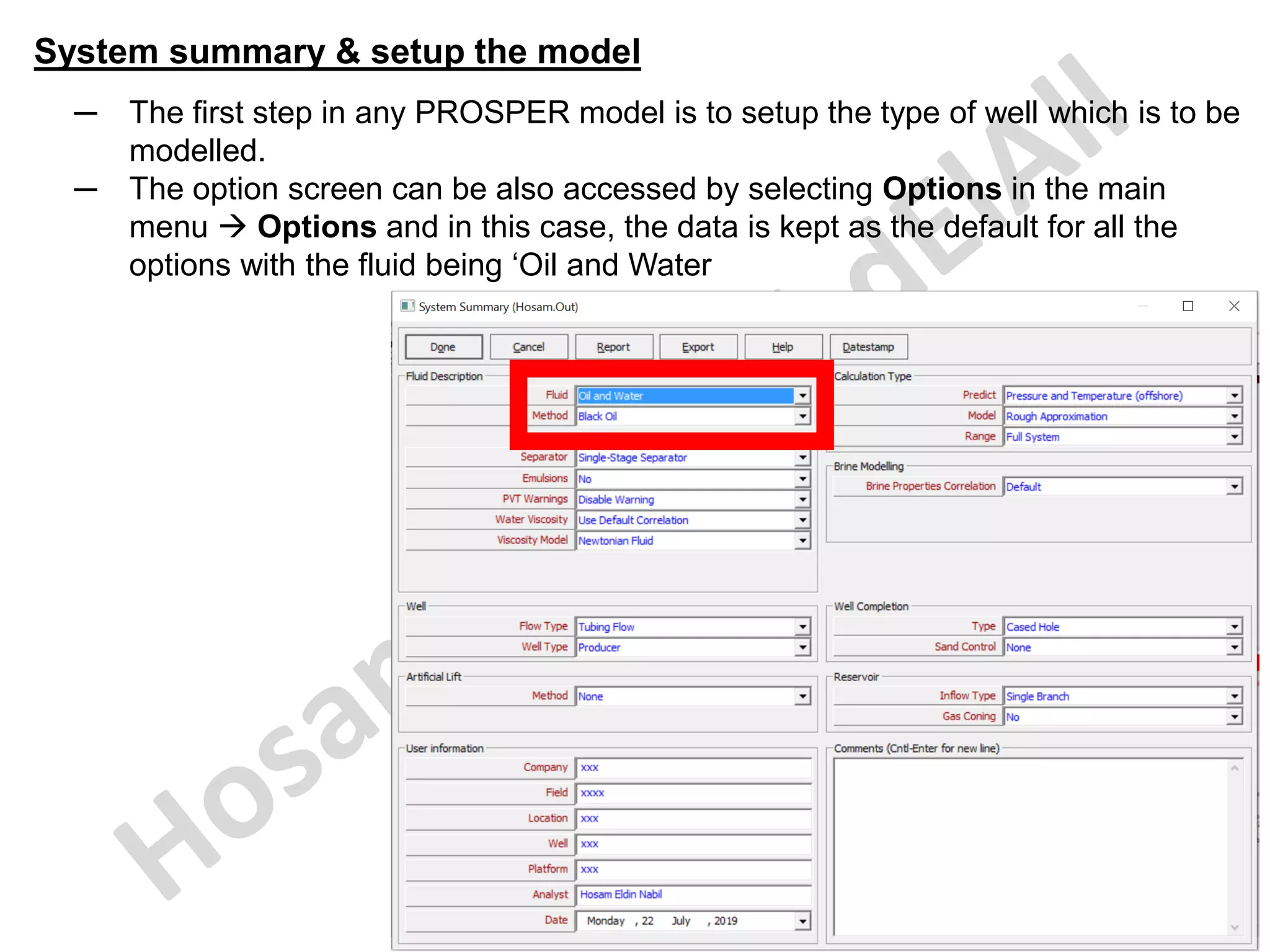
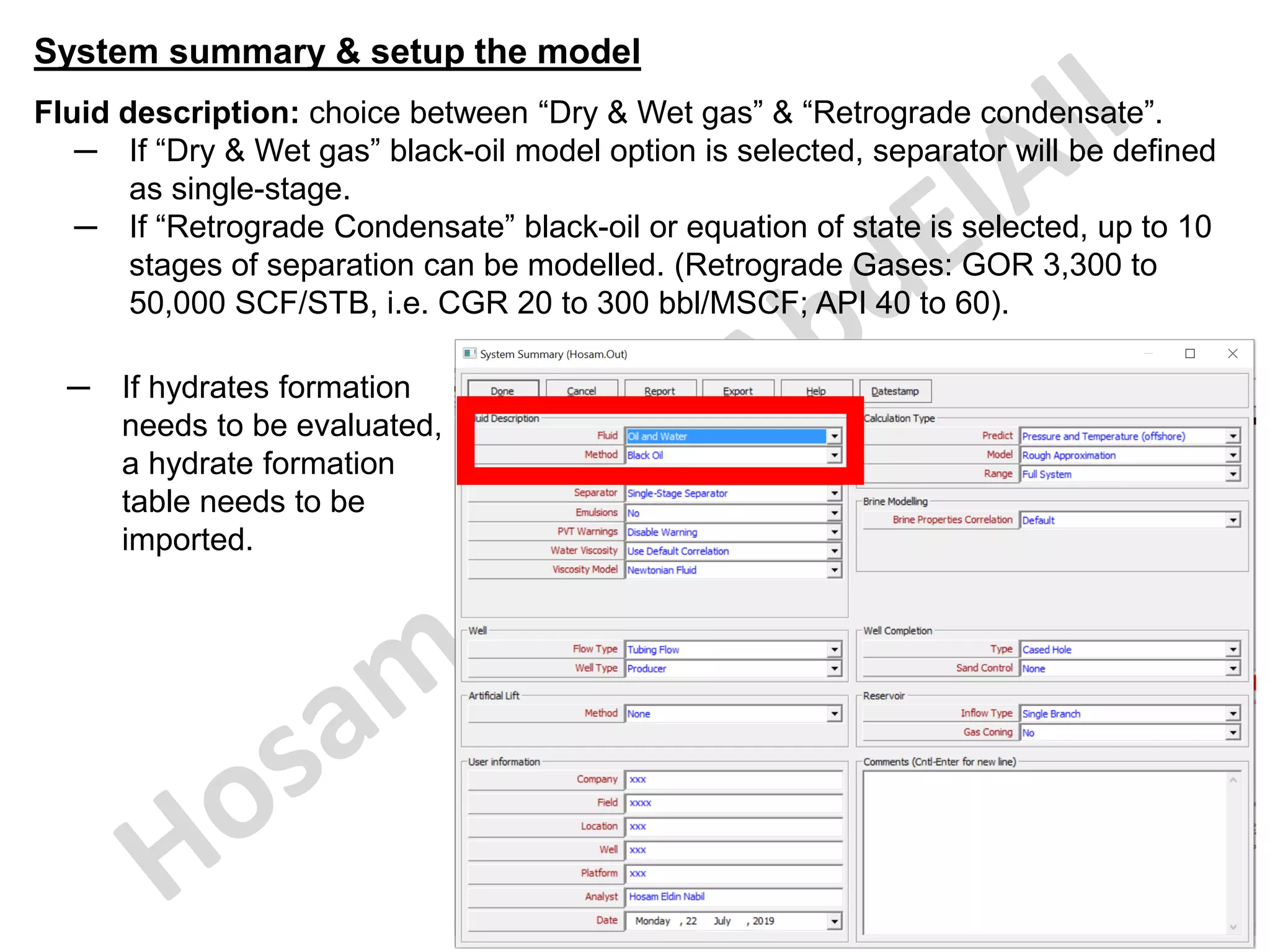
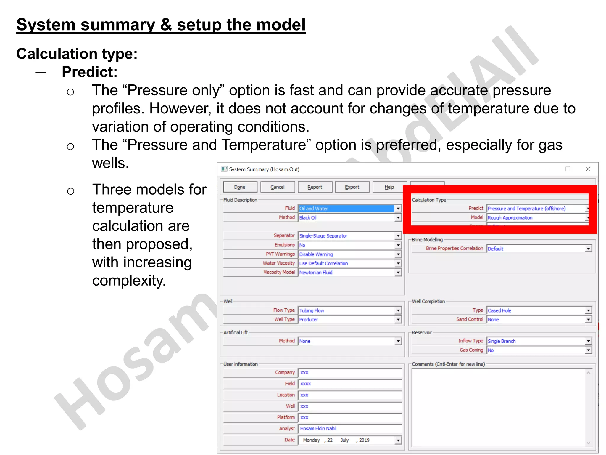
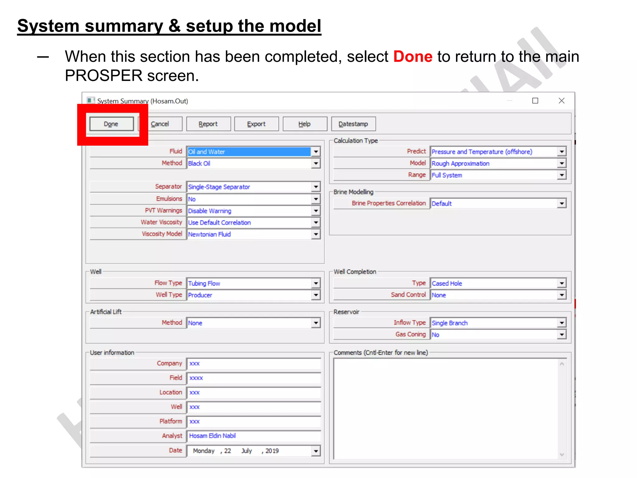
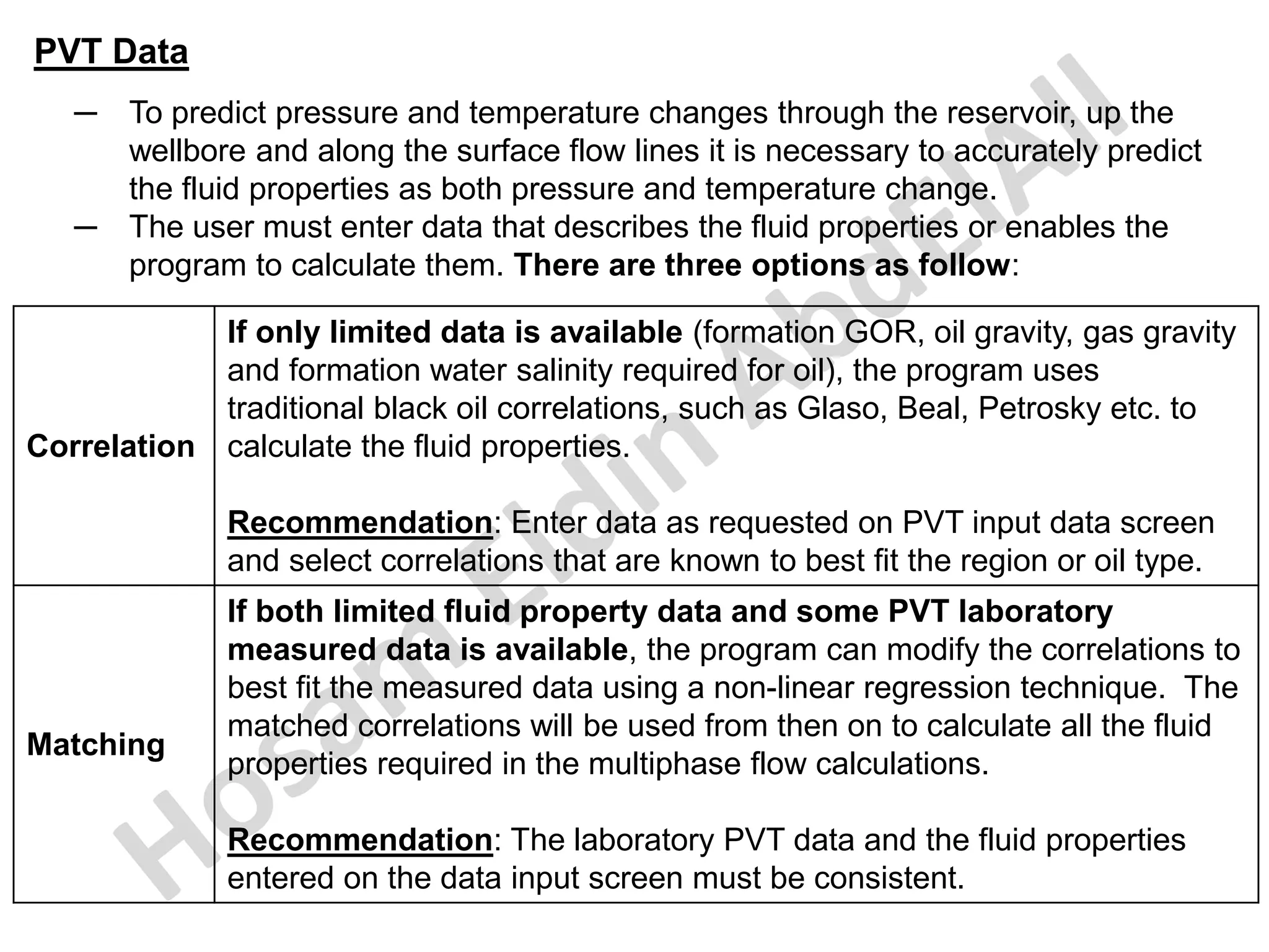
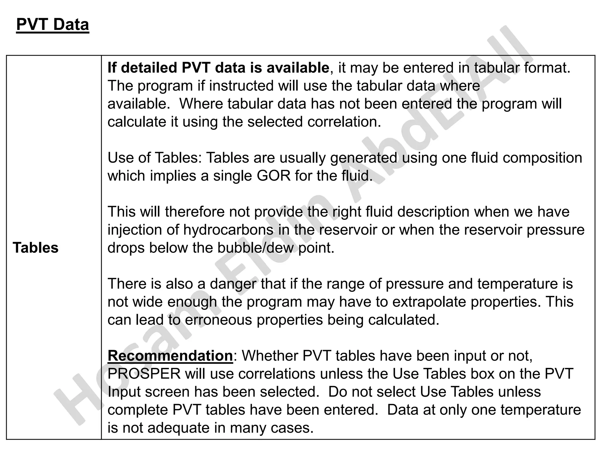
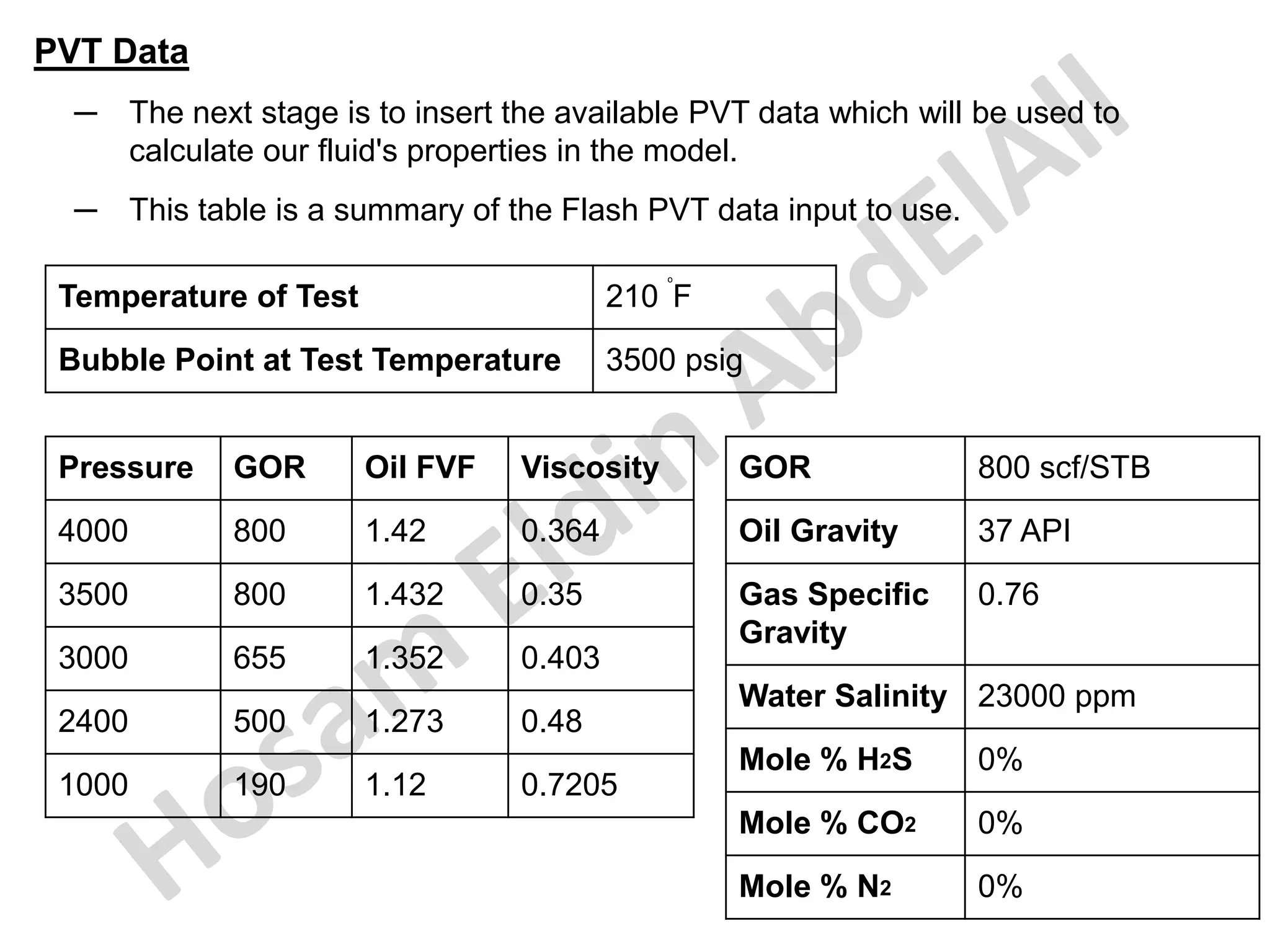
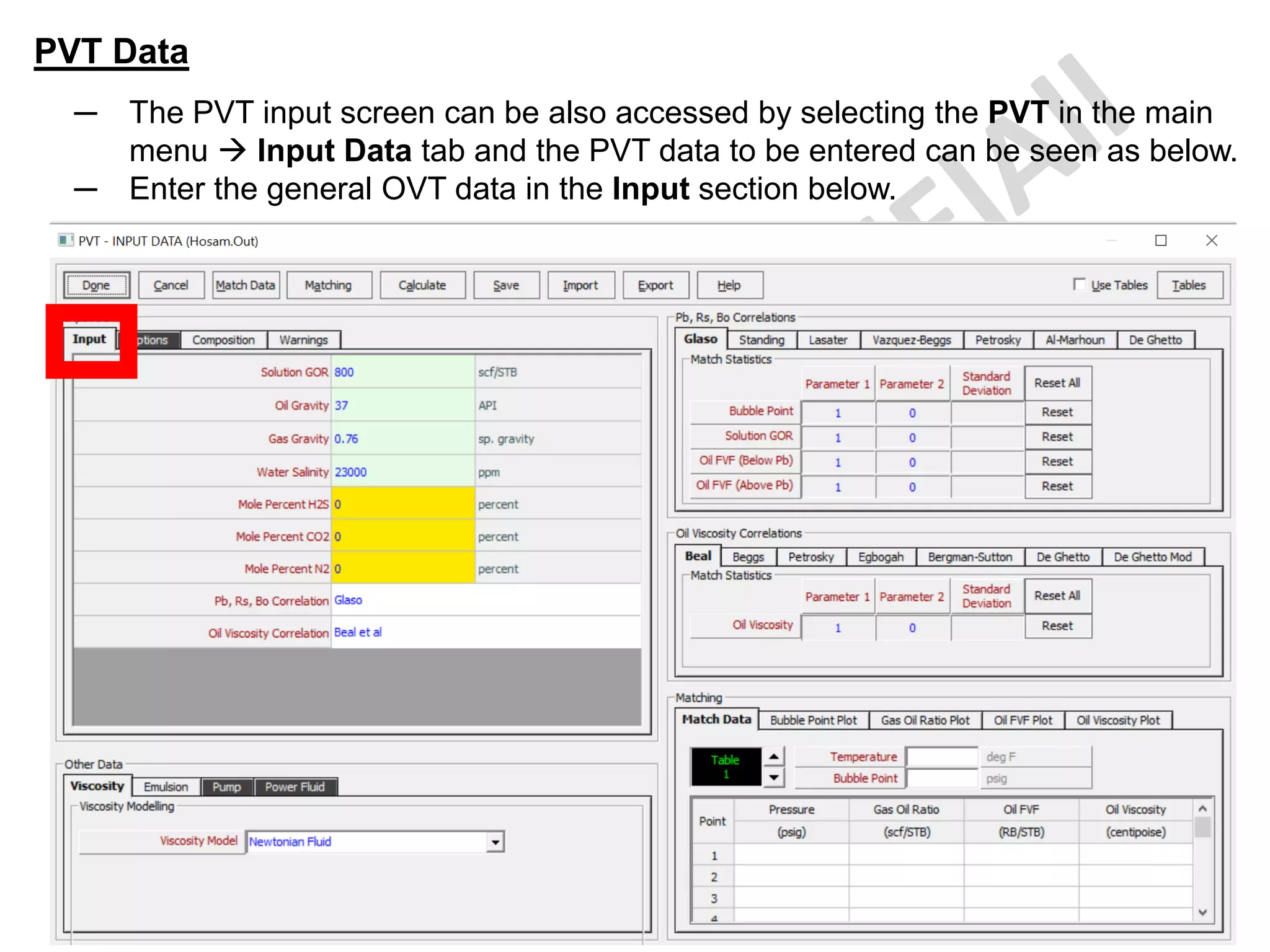
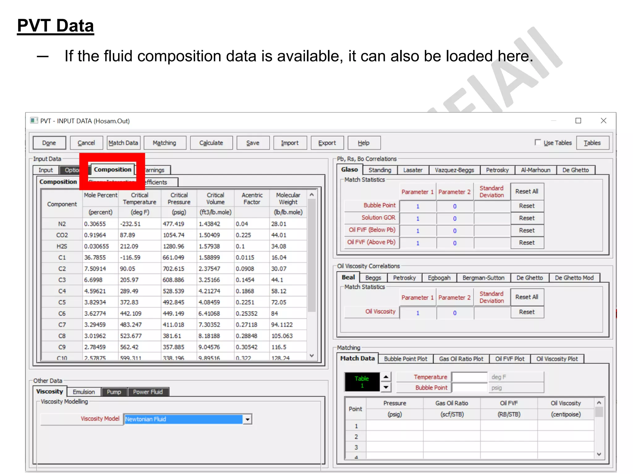
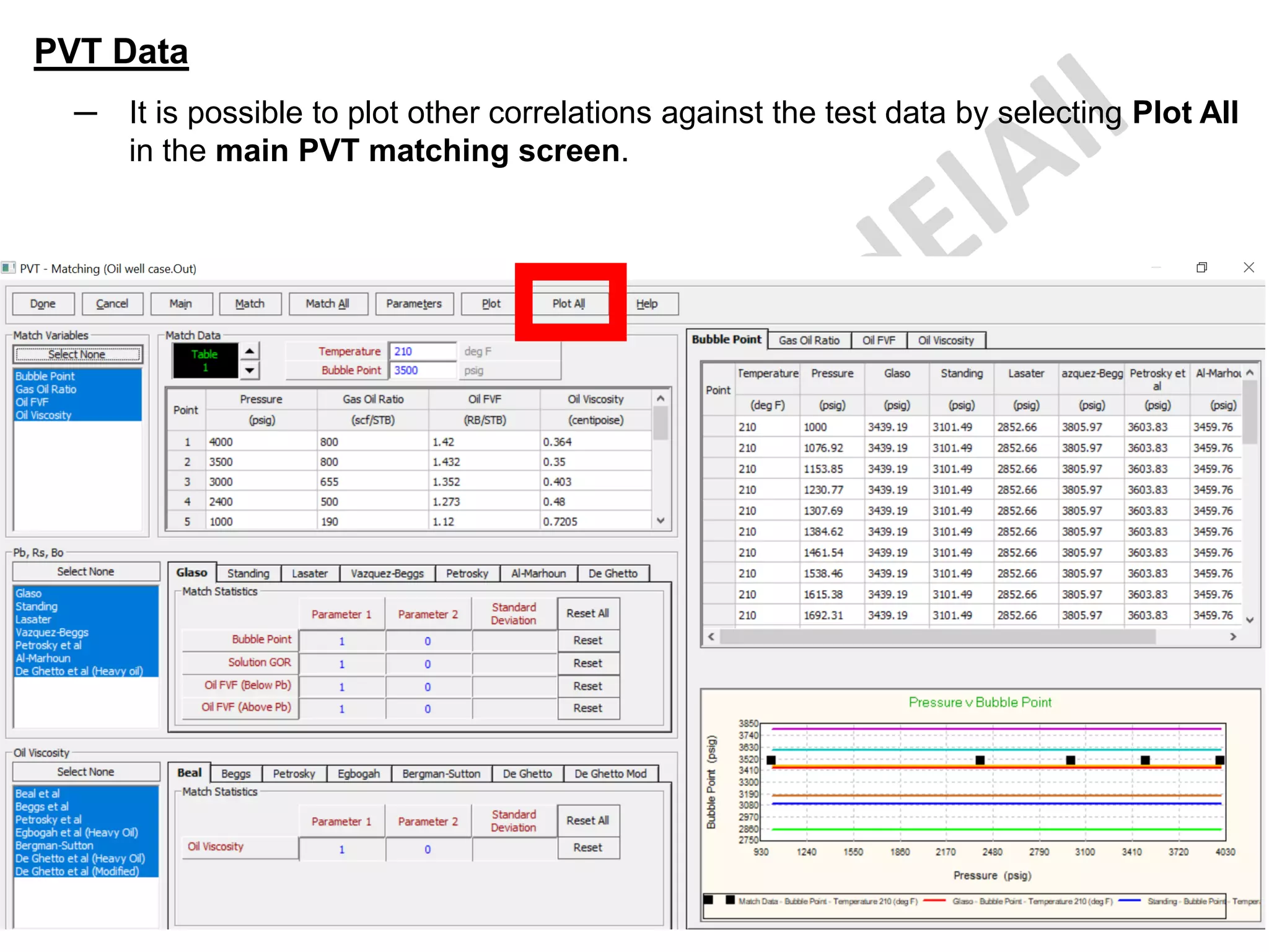
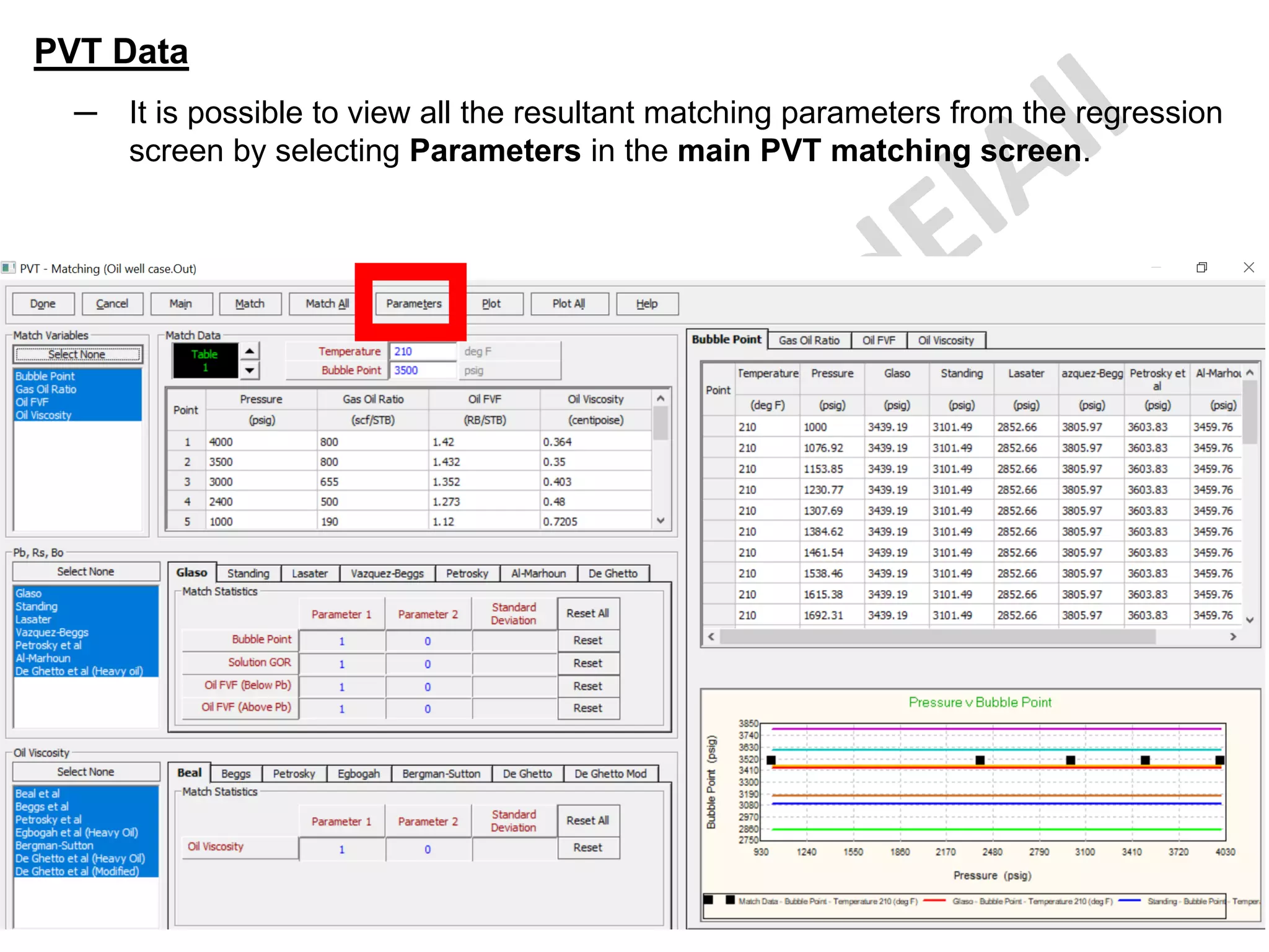
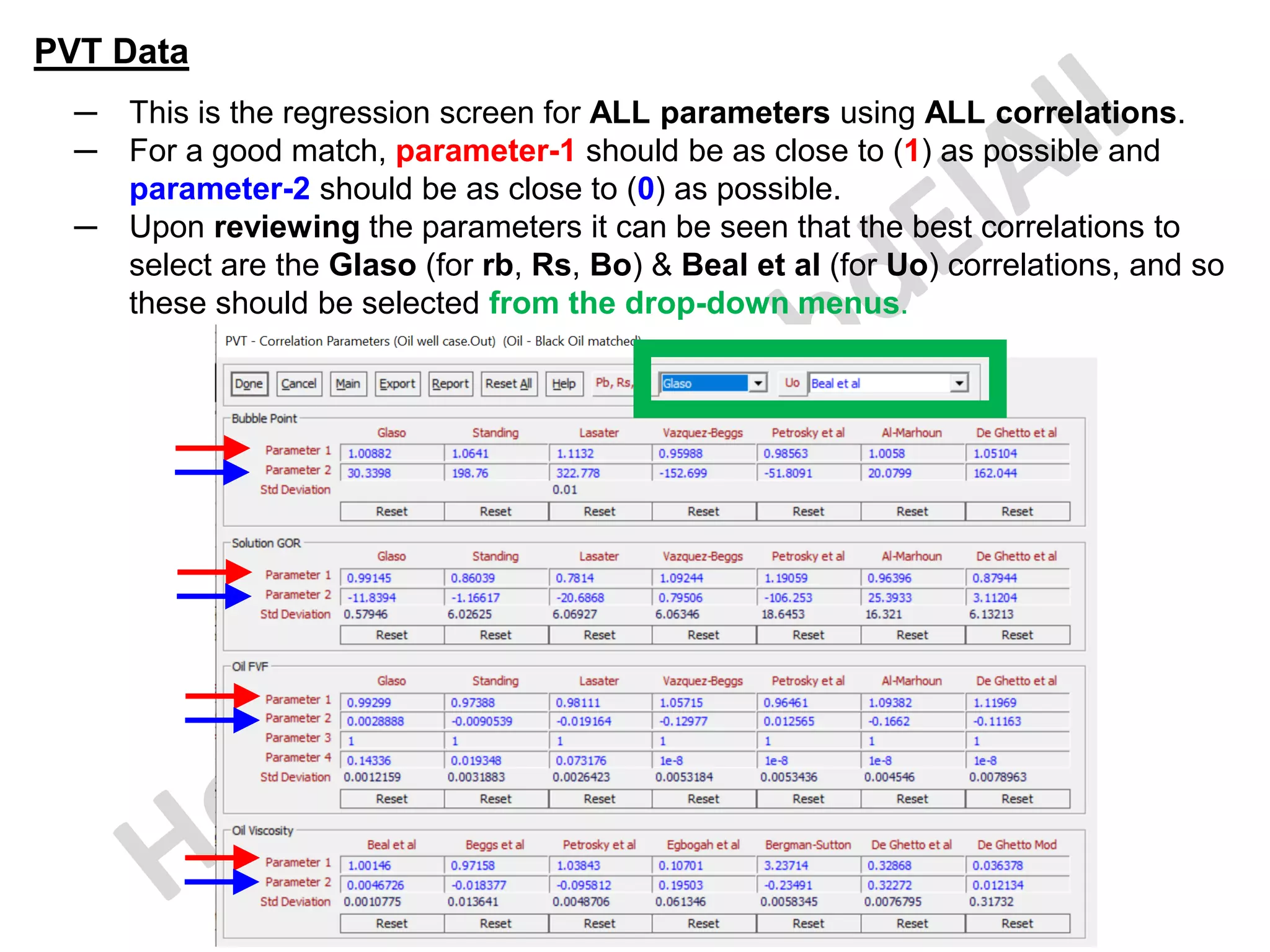
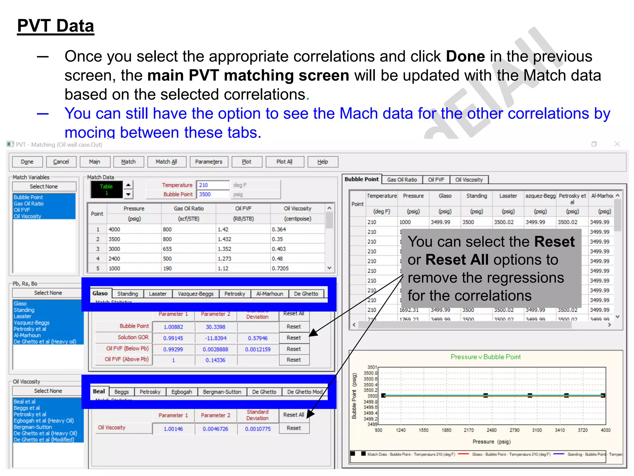
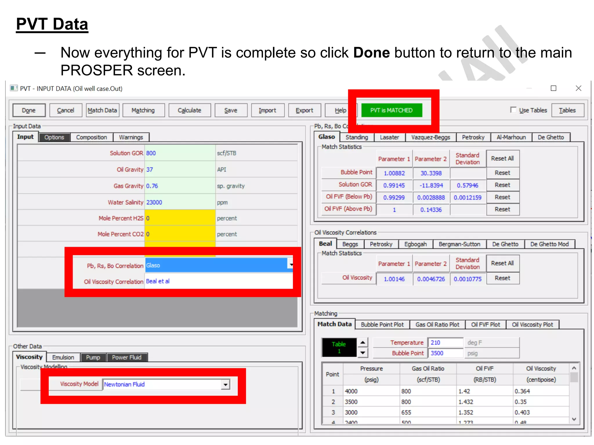
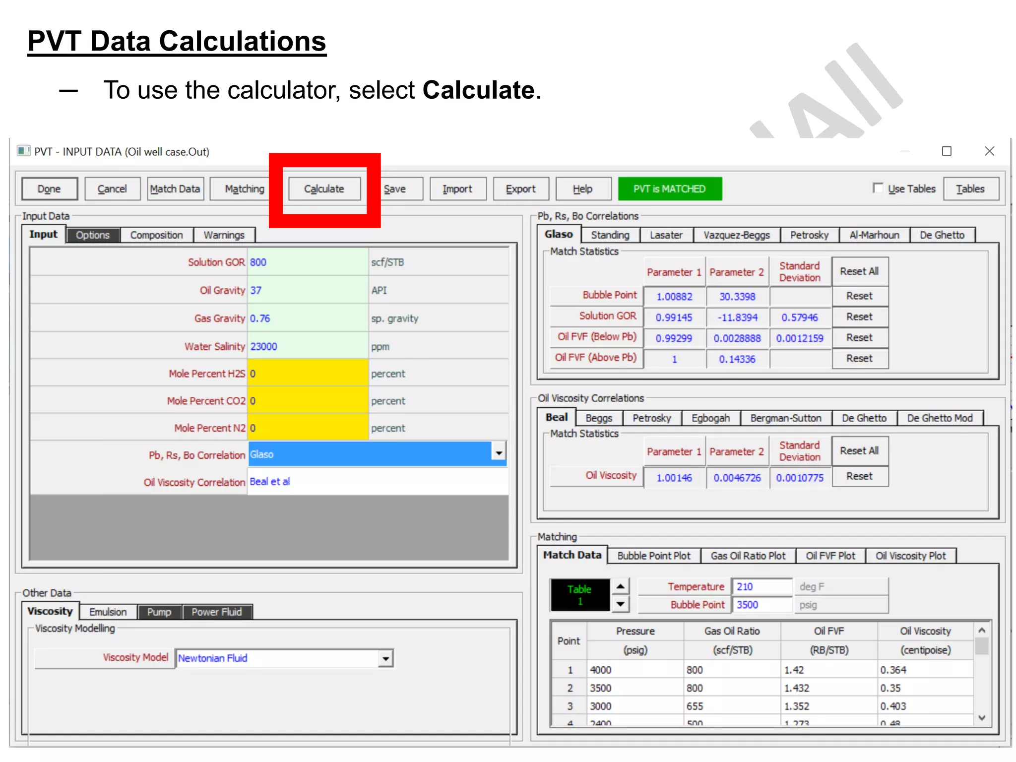
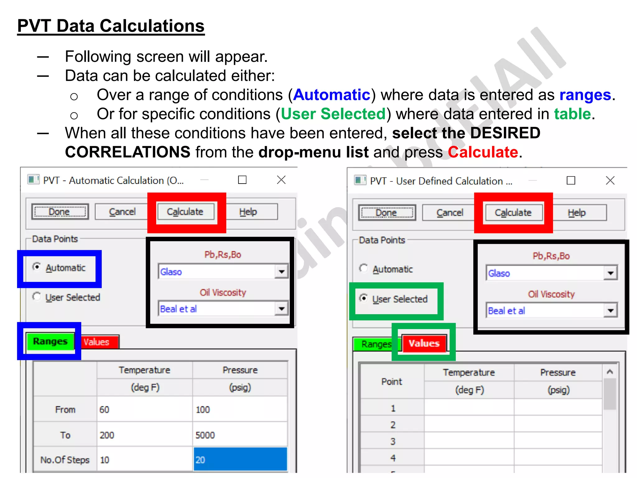
Prosper work example
Oil well case

─ Nodal analysis is a petroleum engineering core technique that is used to
analyze well performance or deliverability.
─ A lot of software's are available in the market for this purpose, one of the
common widely used software used in the market is the “PROSPER”.
─ The outputs from PROSPER models are then used in subsequent
engineering calculations and studies. Therefore, consistent and accurate
well models are necessary in performing and achieving the state-of-the-
art engineering work.
─ Prior to building a PROSPER model for a well, necessary data is
required. This data is acquired during the post completion or surveillance
well tests. Once the data is identified, it should be quality checked and
organized. Then work on the PROSPER modeling can start.

PROSPER models require updates whenever the following well data is
available:
─ Post completion test data should be used as the starting data set for
developing a PROSPER model for the first time. Although it is not a
priority for wells when latest data is available, still it is worth checking the
validity of the PROSPER model with different data sets.
─ Multi rates tests (MRT) data with bottomhole gauge data. This data is the
most important data set that PROSPER model should be calibrated with.
─ Eventually PROSPER will be updated with the daily production data in
cases only a single rate test (SRT) is available or there are no MRT
available for long period of time for a given reason.

Following are some of the technical tasks requires utilization of the
PROSPER models sometimes as frequent as on a daily basis.
─ The immediate application of PROSPER is using the vertical lift curves
(VLP) for each well in running the Production Guidelines on routine basis.
─ Well performance analysis and monitoring (time-lapse performance
change, AOF analysis, skin, reservoir pressure change, etc…).
─ Create vertical lift performance (VLP) curves for simulation models.
─ GAP model, either standalone or as a repository for the ongoing Real
Time Production Optimization Project.
Because of the importance of all above utilization of PROSPER models,
consistently and accurately updated well models are essential.
Following discussion includes the detailed standard procedures that should
be followed to build, calibrate & update a PROSPER well model starting from
data preparation to the last step of the calibration process.

Before you open PROSPER.
─ To build a PROSPER model from scratch or update an existing model, a
data preparation phase is required and it is explained in a step by step as
follow:
─ Fill in an existing and pre-organized EXCEL file. This file is named “input
data for PROSPER”. The file contains three data sheets. These sheets
are organized in such a way to accommodate all wells and all the data
needed for PROSPER. These sheets are named:
o Completion
o Test
o PVT and IPR.

Completion Data.
─ In this tab the tubing lengths and ID are input. The key elements to
consider when filling this table are:
o Only major ID changes are considered
o All depths start from the tubing hanger in MD RKB (not SS)
o Last section depth is the top perforation
The detailed information is obtained from the well schematics shown in next
slide to illustrate how the tubing depths and ID are picked and where the
data is entered in PROSPER

OBJECTIVE
Prosper Modeling aims to assess and predict well production and
performance through simulation by doing the following.
─ Build an integrated oil well which represents the real flowing conditions of
the well.
─ Insert and match PVT data to reproduce the results of laboratory
experiments.
─ Insert the required equipment data to build a VLP curve.
─ Build a Darcy IPR model and include an analytical skin model to account
for the differences between the 'ideal' Darcy reservoir model and the real
life well.
─ Insert the required data to include the impact of a gravel pack on the IPR.
─ Match the VLP curve to test data.
─ Use the matched VLP curve to estimate the reservoir pressure at the time
of the test when the productivity is known.
─ Carry out a sensitivity to see the impact that water cut has on well
production.

System summary & setup the model
─ The first step in any PROSPER model is to setup the type of well which is to be
modelled.
─ The option screen can be also accessed by selecting Options in the main
menu → Options and in this case, the data is kept as the default for all the
options with the fluid being ‘Oil and Water

Fluid description: choice between “Dry & Wet gas” & “Retrograde condensate”.
─ If “Dry & Wet gas” black-oil model option is selected, separator will be defined
as single-stage.
─ If “Retrograde Condensate” black-oil or equation of state is selected, up to 10
stages of separation can be modelled. (Retrograde Gases: GOR 3,300 to
50,000 SCF/STB, i.e. CGR 20 to 300 bbl/MSCF; API 40 to 60).
─ If hydrates formation
needs to be evaluated,
a hydrate formation
table needs to be
imported.

Calculation type:
─ Predict:
o The “Pressure only” option is fast and can provide accurate pressure
profiles. However, it does not account for changes of temperature due to
variation of operating conditions.
o The “Pressure and Temperature” option is preferred, especially for gas
wells.
o Three models for
temperature
calculation are
then proposed,
with increasing
complexity.

Calculation type:
─ Model:
o Rough approximation” is suitable for most routine analysis.
▪ The geothermal gradient should be related to stabilized temperatures
(i.e. extrapolated) and must not be confused with flowing temperatures
required for the “Pressure only” option.
o “Enthalpy balance” and “Improved Approximation” allow considering the
transient effects of temperature.
o The “Improved Approximation” temperature model requires calibration
using measured temperature data. It is not accurate in a predictive mode.
o They require considerably more input data and computation time. This
should be restricted to some particular analysis when a detailed
temperature prediction is required:
▪ Long pipelines;
▪ Subsea wells;
▪ High pressure/temperature wells;
▪ Wax/hydrate deposits analysis;
▪ Joule-Thompson effects.

─ When this section has been completed, select Done to return to the main
PROSPER screen.

PVT Data
─ To predict pressure and temperature changes through the reservoir, up the
wellbore and along the surface flow lines it is necessary to accurately predict
the fluid properties as both pressure and temperature change.
─ The user must enter data that describes the fluid properties or enables the
program to calculate them. There are three options as follow:
Correlation
If only limited data is available (formation GOR, oil gravity, gas gravity
and formation water salinity required for oil), the program uses
traditional black oil correlations, such as Glaso, Beal, Petrosky etc. to
calculate the fluid properties.
Recommendation: Enter data as requested on PVT input data screen
and select correlations that are known to best fit the region or oil type.
Matching
If both limited fluid property data and some PVT laboratory
measured data is available, the program can modify the correlations to
best fit the measured data using a non-linear regression technique. The
matched correlations will be used from then on to calculate all the fluid
properties required in the multiphase flow calculations.
Recommendation: The laboratory PVT data and the fluid properties
entered on the data input screen must be consistent.

PVT Data
Tables
If detailed PVT data is available, it may be entered in tabular format.
The program if instructed will use the tabular data where
available. Where tabular data has not been entered the program will
calculate it using the selected correlation.
Use of Tables: Tables are usually generated using one fluid composition
which implies a single GOR for the fluid.
This will therefore not provide the right fluid description when we have
injection of hydrocarbons in the reservoir or when the reservoir pressure
drops below the bubble/dew point.
There is also a danger that if the range of pressure and temperature is
not wide enough the program may have to extrapolate properties. This
can lead to erroneous properties being calculated.
Recommendation: Whether PVT tables have been input or not,
PROSPER will use correlations unless the Use Tables box on the PVT
Input screen has been selected. Do not select Use Tables unless
complete PVT tables have been entered. Data at only one temperature
is not adequate in many cases.

PVT Data
─ The next stage is to insert the available PVT data which will be used to
calculate our fluid's properties in the model.
─ This table is a summary of the Flash PVT data input to use.
Temperature of Test 210
o
F
Bubble Point at Test Temperature 3500 psig
Pressure GOR Oil FVF Viscosity
4000 800 1.42 0.364
3500 800 1.432 0.35
3000 655 1.352 0.403
2400 500 1.273 0.48
1000 190 1.12 0.7205
GOR 800 scf/STB
Oil Gravity 37 API
Gas Specific
Gravity
0.76
Water Salinity 23000 ppm
Mole % H2S 0%
Mole % CO2 0%
Mole % N2 0%

PVT Data
─ The PVT input screen can be also accessed by selecting the PVT in the main
menu → Input Data tab and the PVT data to be entered can be seen as below.
─ Enter the general OVT data in the Input section below.

PVT Data
─ If the fluid composition data is available, it can also be loaded here.

PVT Data
─ Insert the available PVT test match data in the Match Data tab of the
"Matching" section in the main PVT screen.
Many PVT tables can
be added from here

PVT Data
─ Once this has been done, select the "Match data" button at top of the screen.

PVT Data
─ This will give this screen that shows the PVT test data entered earlier.
─ If u want to see a plot for any parameter with pressure just click Plot and select
the required parameter to show on a plot from the displayed screen.

PVT Data
─ This is the test FVF vs pressure
─ You can change the displayed variable in the plot by clicking this Variables tab.

PVT Data
─ Once this has been done, select the "Match" button at the top of the screen
shown below which will allow us to proceed to the regression screen.

PVT Data
─ OR to have the same screen from the beginning, just select the "Matching"
button at the top of the screen shown below which will allow us to proceed to
the SAME regression screen.

PVT Data
─ On first entering the "Matching" regression screen, the following will be seen.
─ Select Match All at the top of the screen will match ALL the correlations with
ALL the available data.
─ You can select specific test parameter & specific correlation to see the Match.

PVT Data
─ In this case select Match All to match all the correlations and data.
─ As shown below, the matching parameters for each correlation can be seen
and the plots for each property can be viewed for each correlation with respect
to the match data.
This is for example the Bubble
point pressures data & plot
using different correlations
You can see the other
parameters matches with
different correlations
from these tabs

PVT Data
─ Alternatively, by selecting the Plot option it is possible to see the graph of the
matched correlation compared to the laboratory data points.

PVT Data
─ The option of plotting the data is either by Pressure or by
Temperature.
─ Selecting by Temperature will plot each different variable against
pressure and have a different trend line for each temperature.
─ Selecting by Pressure option will show trend lines depending on
pressure and plot against temperature.
─ The correlation which will be shown in the plotting is the correlation
which has been selected in the Correlations section of the above
screen.
─ In this case select by Temperature.

PVT Data
─ This is the displayed screen
To plot the required variable:
• First select the PVT Calculated
Data.
• Then double click the required
variable from here (in this example
select FVF).
• The same should also be carried
out for the PVT Match Data.

PVT Data
─ This is a plot of the FVF data compared with the only selected correlation
output (in this example I selected Glaso & Beal et al correlations).
─ We can see a good match.

PVT Data
─ It is possible to plot other correlations against the test data by selecting Plot All
in the main PVT matching screen.

PVT Data
─ This is a plot of the FVF data compared with the ALL correlations outputs.
You can see the other
parameters matches
with different correlations
from these tabs

PVT Data
─ It is possible to view all the resultant matching parameters from the regression
screen by selecting Parameters in the main PVT matching screen.

PVT Data
─ This is the regression screen for ALL parameters using ALL correlations.
─ For a good match, parameter-1 should be as close to (1) as possible and
parameter-2 should be as close to (0) as possible.
─ Upon reviewing the parameters it can be seen that the best correlations to
select are the Glaso (for rb, Rs, Bo) & Beal et al (for Uo) correlations, and so
these should be selected from the drop-down menus.

PVT Data
─ Once you select the appropriate correlations and click Done in the previous
screen, the main PVT matching screen will be updated with the Match data
based on the selected correlations.
─ You can still have the option to see the Mach data for the other correlations by
mocing between these tabs.
You can select the Reset
or Reset All options to
remove the regressions
for the correlations

PVT Data
─ Now that the correlations have been matched and the parameters and
plots reviewed.
─ It is necessary to select the correlation which is most representative of
the laboratory data.
─ This is done on the main PVT 'Input Data' screen.
─ The correlations in the drop-down menu are those which will be used in
the model and for this oil the Glaso and Beal et al correlations should
be selected.
─ A green banner can also be seen @ top of the page beside the main
menu bar which tells the user that the correlations have been
matched.
─ See next slide.

PVT Data
─ Now everything for PVT is complete so click Done button to return to the main
PROSPER screen.

PVT Data Calculations
─ In order to make a plot or list of fluid property data, PROSPER must first
calculate the values over a specified range of temperatures and pressures.
─ Using the calculated data points based on the selected correlation, plots
of fluid properties versus temperature or pressure can be generated.
─ If the correlations have been matched, then the fluid properties will be
calculated using the modified correlations.
─ The calculation section is used to generate fluid property data for display
and quality control purposes only.
─ During the computation of a pressure traverse, PROSPER calculates fluid
properties at each pressure and temperature step or node as required by
the application.
─ Calculating PVT Data, to generate tables and plots of PVT data:
o Select the Correlations (use the best matched ones)
o Enter the temperature range and number of steps
o Enter the pressure range and number of steps
o Click-on Calculate to calculate the PVT data based on the selected
correlation.

─ To use the calculator, select Calculate.

─ Following screen will appear.
─ Data can be calculated either:
o Over a range of conditions (Automatic) where data is entered as ranges.
o Or for specific conditions (User Selected) where data entered in table.
─ When all these conditions have been entered, select the DESIRED
CORRELATIONS from the drop-menu list and press Calculate.

─ This is the Calculated PVT Data & the generated tables of PVT data based on
the selected correlations.
─ In order to Plots the results of this calculated PVT data (Plots can either be
viewed with pressure or temperature on the X-axis), just click Plot.
─ In this step I selected the plots X-axis to be viewed with pressure.

─ This is the displayed screen for the Plot.
─ The different fluid properties can be plotted by selecting them in the bottom
left-hand corner of the screen.

─ This is the oil FVF vs pressures plot @ these different temperatures.

─ This will be the plot if I selected the plot X-axis to be viewed with
temperatures.
─ This is the oil FVF vs temperatures plot @ these different pressures.

PVT Warning
─ This option allow entering a series of points describing the pressure-
temperature region in which the selected PVT issue (such as Hydrate
Formation, Salt Precipitation, Wax Appearance, Asphaltenes & Scale
Production) is likely to form.
─ This information can be obtained from a study of your hydrocarbon fluid
using Petroleum Experts' PVTP program.
─ Up to 100 pairs of data points can be entered and plotted.

PVT Warning
─ To accesses this option, PROPSER main menu → PVT → PVT
Warning.
Select Enable Warning
beside any conditions that
may be an issue in the field
Click the Data button
beside the selected
conditions to add the
required data for this
condition

PVT Warning
─ For this example, I selected the Hydrates formation that may be an
issue in the field.
─ Click Plot.

PVT Warning
─ This is the Hydrates formation plot.

PVT Warning
─ The same PVT Warning can be found in the PROPSER main menu →
PVT → Input Data.

Specifying Equipment Data
─ In order to calculate the VLP curves for the well, PROSPER must have a
description of the well and the path through which the fluid flows from the
bottom of the well to the wellhead. This is done in the 'Equipment Data' section.
─ it can be also accessed by selecting System in the main menu → Equipment
(Tubing etc).
─ This will bring up the 'Equipment Data' screen.
─ In order to fill in data
for all the appropriate
sections select All from
the top ribbon and this
will bring up ticks next
to each section.
─ The Edit button can
now be selected to
bring up each input
section one at a time.
─ To move onto the next
input screen, select
Done.

Specifying Equipment Data
─ To start the data entry for a new application, click All button to select all the
different sections and click the Edit button will then display all the relevant input
screens in sequence.
─ If data has already been entered, and only one section is to be edited (for
example edit downhole equipment), the required section can be accessed by
selecting the square to the left of the ticked box corresponding to that section.
─ Data can be entered for the
surface equipment and then
include or exclude it
temporarily from any
calculation by setting the
Disable Surface Equipment
choice box at the bottom of
the screen to Yes.
─ If data has already been
entered, clicking the
Summary command button
will display a summary of the
current equipment.
─ When finish click Done to
return to the main menu.

Specifying Equipment Data - Deviation Survey
(Tubing etc).
─ Select the checkbox beside the Directional survey then click Edit button.
You can click this
square to Edit the
data directly.

─ In this screen the well deviation
survey is added.
─ it can be also accessed by selecting
System in the main menu →
Equipment (Tubing etc.) → select
Direction Survey in the opened
window → EDIT
─ From the well deviation survey, select
several depth points that mark
significant changes in deviation.
─ Enter pairs of data points for
measured depth (MD) and the
corresponding true vertical depth
(TVD). Up to 20 pairs of data points
can be entered.
─ Then PROSPER will calculate the
cum. Displacement & the Angle.

─ There is a Measured Depth to True
Vertical Depth calculator at the top
of the screen.
─ This option is to calculate the TVD
for the known MD value & vise versa.
─ If the user wishes to find the TVD at
a given MD, just enter the MD value
in the relevant space & select
Calculate.
─ Once depths have been entered, plot
the well profile by selecting Plot. A
plot like the one in the next slide will
be displayed.
─ When finish click Done to return to
the main screen.

─ This is the plot of the entered MD & TVD data vs the calculated Cumulative
Displacement .

─ The reference depth used by PROSPER for all calculations is zero in the Deviation
Survey table.
─ The deviation survey has to start with (0) measured depth & (0) TVD. Due to this
reason, the reference depth (where TVD = 0) has to be @ or above the wellhead.
─ For a sub-sea well (with or without pipeline), if the reference depth is selected in
such a way that it is above the wellhead (at the mean sea level for instance), we
can assume an imaginary vertical path in the deviation survey table down to the
wellhead. We do not need to include the pipeline measured depth in the deviation
survey. The deviation survey describes the deviation of the down-hole equipment
only.
─ MD and TVD data must be at least as deep as the bottom-hole tubing depth;
PROSPER will not calculate beyond the last depth in the table.
─ Deviation Survey data entry is required also for vertical wells - enter (0 , 0) for
the surface reference and MD the same as the TVD of the intake node.
─ Horizontal wells with deviation angles greater than 90 degrees from vertical can be
entered. PROSPER will issue a warning that the TVD of one node is less than the
previous one, but well profile plots and calculations will proceed as normal.
─ For Horizontal wells the deviation survey may be entered only up to the heel of the
well (at the end of the bend curve), as the well from the heel all the way up to the
ending point is a part of the inflow description.

Specifying Equipment Data ─ Deviation Survey ─ Filter
Note that:
─ If the deviation survey has more
than 20 data points, it is possible
to reduce the number of points
using a filter algorithm.
─ When selecting Filter, the program
will filter the points in order to
reproduce the well trajectory.
─ This Filter option allows a
determined number of points (up to
20) that best-fit the entered points.
─ This option is accessible by
selecting the Filter button that
have a feature to fit deviation
survey with up to 1000 points.

─ Select Raw Data Type
(MD/TVD, TVD/Angle or
MD/Angle)
─ Enter the data from the survey
in the Raw data table. It is
possible to copy the survey
data then select the first row in
the Raw data table and paste
from the Clipboard.
─ Calculate Other: to calculates
the other unknown parameter
by knowing the two parameters
entered in the Raw Data Type.
For example, If MD/TVD was
used, then it will calculate the
angle of deviation from vertical.

- The Filter parameters are described in the following table:
Initial Filter
Angle
Used to chose second point of the deviation survey; the point with
higher angle will be filtered through
Angle Step Defines the minimum angle difference between two points; if the
difference is higher the point will be filtered through
Maximum
Number of
Points
• The Maximum Number of Points that can be filtered through
• If the number of points filtered is more than the value specified
PROSPER will increase the angle to satisfy the criterion
Actual Filter
Angle
The angle calculated by PROSPER to satisfy Maximum Number of
Points criteria
- Besides the standard buttons there are some additional buttons:
Reset Deletes the entered data
Filter • Calculates several points which fit the deviation table entered
in the Raw Data Type. Check the fitting by hitting on Plot.
• If this is not ok, change some parameters (like for example the
Initial Filter Angle) until the match is reached
Transfer Transfers the calculated points to the main Deviation Survey screen

─ The filtering is performed on the basis of Measured Depth (not Cumulative
Displacement). In essence, the filtering ensures that the measured depth (and
TVD) between two points is always consistent with the original survey even
though plotted profiles may appear slightly different. This is because
Measured Depth defines length of the pipe (tubing), which is particularly
important in temperature and pressure drop calculations in PROSPER.
─ The first point of the deviation survey is always filtered through as a starting
point.
─ Then the Initial Filter Angle parameter is used to choose second point of the
deviation survey; i.e., the first point along the deviation survey where the angle
from the vertical goes above the initial filter angle will pass through the filter
and is selected as the second point.
─ The next points are filtered through based on the Angle Step; i.e., if the
difference in the angle between two points is more than the value specified.
─ PROSPER calculates the Angle Step internally depending on the Maximum
Number of Points entered by user; i.e., if the number of point passed through
the filter is more than the Maximum Number of Points specified the angle will
be increased to satisfy the former. The resulting value is then reported as
Actual Filter Angle.

─ After clicking the Filter button
and the filtered data is updated
in the Filtered Data table then
you have to check these new
calculations that it matches wit
the original deviation survey.
─ Just click on Plot button to do
this quality check the fitting by
comparing the new calculations
that it matches wit the original
deviation survey on a plot (see
next slide).

─ In the plot the well entered trajectory (in blue) is plotted along with the fitted
points (in red).
─ This is comparison of the new calculations that it matches wit the original
deviation survey plot that shows an excellent match.

Specifying Equipment Data ─ Surface Equipment
(Tubing etc).
─ Select the checkbox beside the Surface Equipment then click Edit button.
You can click this
square to Edit the
data directly.

─ The Surface Equipment screen is used to enter surface flowline, choke & pipe
fitting data as shown below.
─ Data is entered from the manifold (@ the top of the screen) to the wellhead
(@ the bottom of the screen).
Select the desired
choke correlation
model to calculate
the choke
performance curve.
It is recommended to
use the ELF Choke
correlation since it is
more robust in
extreme conditions.
Ensure that this depth of the most upstream point
defined in the Surface Equipment (which connects to the
Xmas Tree) is the same as the Xmas Tree depth defined
in the Downhole Equipment to avoid any error message.

─ It is possible to import pipe ID values from Pipe Schedule databases by click
the Pipe Schedule button then select the type of pipe from the database →
copy → done.
@ the bottom in the
displayed screen,
select Copy ID and
OD to Selected
Records, then
Done, this will pass
the values to the
equipment screen
here.

─ The surface equipment model can be described using the following 4 elements.
Pipe Segment of pipe
Choke
• A multiphase choke correlation is used which is valid for both
critical and subcritical flow.
• The choke model to be used can be selected on this screen. If the
Norsk Hydro model is selected further input will be required. (Use
the Choke Data button). We recommend using the ELF choke
method.
• N.B. The choke model selected in the surface equipment window
will be used to calculate the dP for restrictions and SSSV's in the
downhole equipment window.
Fittings It allows to determine the dP associated to a wide range of fittings
Pump
A multiphase pump can be entered provided this has been setup in
the system summary screen
N.B. When specifying the pump in the surface equipment it should be noted that the
pump cannot be specified next to the wellhead or manifold.
If your configuration requires this then specify a small length of pipe (1 ft) in order
that the fluid properties are set up correctly.

─ PROSPER defines surface equipment as the pipe work between the
production manifold and the upstream side of the wellhead choke.
─ The production manifold is regarded by PROSPER as presenting a constant
back-pressure, regardless of flow rate.
─ If systems analysis is to be performed relative to the wellhead, (i.e., gathering
system pressure losses are neglected) then no surface equipment input is
required.
─ The manifold is set as the first equipment type automatically by PROSPER.
─ Surface equipment geometry can be entered either as pairs of X, Y
coordinates relative to the manifold or the Xmas Tree, Reverse X, Y (Y
coordinates deeper than the reference depth are negative) or TVD of the
upstream end and the length of the pipe segment.
─ The difference in TVD between the ends of a pipe segment is used to
calculate gravity head losses.
─ The internal diameter (ID), roughness and pipe length entered determine the
friction pressure loss.
─ The flowing temperatures for each upstream node must also be entered when
calculation option Pressure only is selected.

─ Ensure that the length of each pipe segment is equal to or greater than the
difference in TVD between its ends.
─ The surface equipment entries must describe a continuous system.
─ The TVD and temperature of the upstream end of the last pipeline segment
should be equal to the X-mas tree TVD and temperature. In X,Y co-ordinates,
the Y co-ordinate of the last pipe segment must be the same elevation as the
wellhead TVD. (i.e., same magnitude, but opposite sign)
─ The Rate Multiplier column enables simulation of the pressure drop due to
several identical wells being connected to a production manifold via a common
surface flow line. The fluid velocity in the flowline is multiplied by the value
entered increasing the frictional pressure losses. For most applications it
should be left at its default value of (1).
─ As an examples for the Rate Multiplier:
o The pressure drop in a flowline connected to 3 identical wells could be
modelled using a pipeline rate multiplier of (3).
o 2 parallel flowlines having identical dimensions can be modelled by entering
the actual dimensions for one pipe and a pipeline rate multiplier of (0.5).
o It is also possible to vary the rate multiplier along the pipeline to simulate
varying sections of dual pipelines for example.

─ Fittings have been added to the surface equipment section of PROSPER to
account for the various pressure losses associated with pipe fittings
throughout a given system.
─ Prosper can model pressure ( and temperature) drop across a range of
fittings.
─ These pressure drops are handled using the equivalent length concept from
which it is possible to determine the corresponding pressure drop as in the
following equations.
Where (h) is the decrease in static head (ft) due to velocity
(ft/sec) and is defined as the velocity head.
─ If a valve or fitting is incorporated in the pipeline the equivalent length is:
Where (K) is the resistance coefficient which is defined as
the number of velocity heads lost due to the valve or fitting.

─ The (K) values are tabulated for a wide range of fittings and configurations.
Select the desired Valve
type from here
Specify the desired Valve
dimensions from here

─ To check that the surface equipment description is accurate, click Plot @ the
top of the main Surface Equipment screen to display a plot of the pipe
elevation as shown below.

Specifying Equipment Data ─ Downhole Equipment
(Tubing etc).
─ Select the checkbox beside the Downhole Equipment then click Edit button.
You can click this
square to Edit the
data directly.

─ The Downhole Equipment section defines the path through which the fluid will
flow as it is produced up the well bore.
─ The Downhole Equipment screen enables the down-hole completion data to be
entered.
─ Downhole Equipment screen will change automatically based on the options
selected in the PROPSER main menu screen toolbar → Options → Options.
─ For example, if Annular Flow is selected when define the well, then the screen
will require Casing I.D. & Tubing O.D. to be entered in addition to Tubing I.D.

─ In my example here I defined the Tubbing flow for the well.
─ In this case the tubing string can be modelled using the following element types
(Tubing, SSSV, Restriction & Casing).
─ PROSPER automatically insert Xmas tree as the first downhole equipment item.
─ To describe the tubing string, work from the shallowest depth downwards,
entering the bottom depth of changes in tubing diameter, ID & roughness factor.
─ The deepest depth entries for the tubing, deviation survey and temperature
should be consistent.
─ The last depth specified in the down-hole equipment is taken to be the bottom-
hole depth by PROSPER and should correspond to the top of the
perforations or the top of the reservoir. This last depth from the down-hole
equipment will be used as the solution node depth which splits the well into
the VLP & IPR. Everything below this depth is considered as part of the IPR.
─ This depth is normally defined as the top of the perforations and thus this
equipment description should stop at the top of the perforations.
─ This depth is also therefore the depth at which the static reservoir pressure is
defined in the IPR section.
─ When the data has been inserted, the next input screen can be accessed by
selecting Done.

─ Below the uppermost producing perforation, the flow profile (as measured by a
production logging tool) depends on layer productivity etc.
o The uppermost producing perforation is the deepest point in the well
passing 100% of the production.
o Below this point, the calculated frictional pressure gradient may be over-
estimated in high rate wells having small I.D. completions.
─ Casing is treated the same as tubing for pressure drop calculations.
o Only enter a downhole equipment description down to the producing
interval being analyzed. i.e., the deepest casing depth entered should be
the point of the producing perforations and equal to the depth of the
reservoir pressure reference.
o The deepest depth entries for the tubing, deviation survey and temperature
should all be consistent.
─ The Rate Multiplier column enables simulation of the pressure drop due to
intermittent sections of dual completion.
─ The fluid velocity in the tubing is multiplied by the value entered - thereby
increasing the frictional pressure losses.
─ For standard single tubing completion, it should be left at its default value of (1).

─ Note that, up to 50 tubing string elements can be input.
─ For complex completions, simplify the data entry by entering only the major
elements that dominate the overall tubing pressure drop.
─ Details of the Downhole equipment to be installed can be found in the table
below.
Type MD (ft)
Inside
Diameter
(Inches)
Inside
Roughness
(Inches)
Rate
Multiplier
X-mas Tree 100 1
Tubing 1000 4.052 0.0006 1
SSSV 3.72 1
Tubing 9000 4.052 0.0006 1
Casing 9275 6.4 0.0006 1

─ This can be inserted (either by typing or by right click on a row in the table then
paste from a copied data from external table) as shown in the screen below.
Select the downhole
equipment component
from this drop menu
for each row
Ensure that this depth of the Xmas
Tree depth defined in the Downhole
Equipment is the same as depth of
the most upstream point defined in
the Surface Equipment (which
connects to the Xmas Tree) to avoid
any error message.

─ It is possible to import tubing & casing ID values from tubing & casing databases
by selecting the type of equipment from the database → copy → done.
Select any cell to copy the required
information from Tubing or Casing
database buttons above

─ Note that this tubing end (9000 ft) is set by default in PROSPER as the top of
perforations @ which the reservoir pressure will be defined.
This depth may be different than the gauge depth that may be hanged or set
away from the tubing end (in this example it was hanged @ depth 6250 ft)
and in this case the extrapolated pressure value @ rate = (0) in the liquid rate
vs. BHFP plot is different than the calculated reservoir pressure @ tubing
end due to gradient difference.

Specifying Equipment Data ─ Geothermal Gradient
(Tubing etc).
─ Select the checkbox beside the Geothermal Gradient then click Edit button.
You can click this
square to Edit the
data directly.

─ The geothermal gradient (GG) which is entered is the geothermal gradient
of the rock around the well.
─ It is used to calculate the temperature difference that the fluid experiences as
it travels up the well and is used in the calculation of heat transfer.
─ TRes (°F) = GG x Depth (ft TV D/SS) + surface temperature (°F)
─ PROSPER interpolates temperatures from the survey data for depths within
the table limits and uses linear extrapolation elsewhere.
─ To eliminate potential errors, ensure that a temperature is entered for the
deepest node depth.
─ It is recommended that the maximum temperature survey depth, deviation
survey depth and intake node depths are all consistent.
─ The heat transfer coefficient should not be confused with the pipe thermal
conductivity. The overall heat transfer coefficient accounts for the heat flow
through the production tubing, annulus and insulation (if present) to the
surroundings. Heat transfer by forced and free convection, conduction and
radiation must all be accounted for in the value of the overall heat transfer
coefficient. In PROSPER, the overall heat transfer coefficient is referenced to
the pipe inside diameter.

─ This screen enables entry of the flowing temperature profile of the fluid in
the well. If no bottom hole flowing temperature survey data is available, the
static reservoir temperature at the mid-point of perforations and the
wellhead flowing temperature can be used.
─ A minimum of two depth / temperature points is required
─ The Overall Heat Transfer Coefficient (U) is also input into this screen and
the value should account for the heat transfer from the fluid to the
surroundings. Its unit is BTU/h/ft2/°F.
This depth is the wellhead
(X-tree) depth that should
be the same as the last
depth entered in the
surface equipment
section which is also the
same as the first depth
entered in the downhole
equipment section.

─ These 3 depths should be the same.

─ To see the Geothermal Gradient plot just click Plot in the Geothermal
Gradient input screen.

─ This is the Geothermal Gradient plot.

Specifying Equipment Data ─ Heat Capacities (Cp)
(Tubing etc).
─ Select the checkbox beside the Average Heat Capacities then click Edit
button.
You can click this
square to Edit the
data directly.

Specifying Equipment Data ─ Heat Capacities (Cp)
─ The average heat capacities of water, oil and gas are used in the Rough
Approximation temperature model to calculate the energy which is provided
when the fluid changes temperature.
─ Note that for oil, and especially gas that Heat Capacities (Cp) values are
strong functions of both temperature & pressure.
─ These are to be kept equal to the default values (0.51 BTU/lb/°F for gas, 0.53
BTU/lb/°F for oil & 1 BTU/lb/°F for water).

Specifying Equipment Data ─ Gauge Details
(Tubing etc).
─ Select the checkbox beside the Gauge Details then click Edit button.
You can click this
square to Edit the
data directly.

Specifying Equipment Data ─ Gauge Details
─ It is possible to enter the depths of different gauges in the PROSPER file.
─ Up to 10 gauges can be added to a well in PROSPER:
─ If gauges are added, the pressure and temperature at the gauge depth will
be given as a reported additional result in any calculations being run such as
VLP are completed.
─ After updated with the gauge depths
data, then select Done to return to
the main 'Equipment Data' screen.
─ If there is no gauge depths data to
add, then leave it blank and select
Done to return to the main
'Equipment Data' screen.

Specifying Equipment Data ─ Equipment Summary
─ From the equipment input screen it is possible to see a summary of the
equipment by selecting the Summary button on the top right of the screen.

Specifying Equipment Data ─ Equipment Summary
─ This is the summary of the equipment.
Click this button to draw the downhole
equipment as shown in this figure

Inflow Performance (IPR)
─ Inflow Performance Relationship (IPR) defines the flow into the well
from the reservoir. Calculating an IPR results in a relationship between
the bottom hole pressure and the flow rate passing into the well.
─ The IPR section of PROSPER defines the inflow of the well and
therefore how productive the reservoir is.
─ There are over 20 IPR models available in PROSPER that can be
selected from the Reservoir Model screen. Each model is applicable to
a different situation or series of conditions.
─ The current reservoir properties such as reservoir pressure and
temperature, water cut and producing GOR can be entered in the
Reservoir Data section.
─ In this case, the PI reservoir model should be selected, which allows
the PI to be entered in the model data screen as shown in the next
slide.
─ The IPR main data input screen can be also accessed by selecting
System in the PROSPER main menu toolbar → Inflow Performance.

─ The screen consists of 5 main parts:
1
2 3 4
5

1. Action Buttons: buttons which perform various actions such as 'Validate' the
input data, 'Calculate' an IPR and 'Plot' the results. The most important Action
Buttons in the screen are:
─ Validate button: checks that the data on the current child screen falls within
the validation ranges of each variable. If the data is not valid, the validation
dialogue will appear with diagnostic messages. If any data is missing, then this
is also highlighted.
─ Calculate: saves and validates all the data pertaining to the chosen models
(e.g., Darcy reservoir model and Enter Skin By Hand) then runs the correct
calculation routine if the data are valid. On successful completion of the
calculation the results are automatically plotted
─ Test Data: Allows to enter test data (rate vs Bottom Hole Pressure, a date
stamp and a comment) that will be then displayed in the IPR plot.
─ Sensitivity: Allows to perform sensitivities on the various parameters affecting
the IPR
─ Transfer Data: saves and validates all the current data before opening a
standard ‘File Save As’ dialogue that provides an opportunity to save the data
to file in MBAL input format (.MIP).

2. Reservoir Model: in this area the main parts of the model are defined
including the IPR model, which (if any) skin models and sand control devices
are being used.
─ The 'model selection' part of the IPR input screen controls the choice of almost
all the tabbed dialogues that will be seen in the model data section.
─ There are four major selections done in this screen. These are:
o Selection of Reservoir Model: for each fluid various single well IPR
models available to be selected.
o Selection of Mechanical/Geometrical Skin Model: the user has the
option of entering the skin by hand or using one of the analytical models
to model the mechanical and geometric skin.
o Selection of Deviation / Partial Penetration Skin Model: there are
three skin models, and these become available if any analytical skin
model of mechanical / geometric skin calculation has been used.
o Enabling sand control devices and specifying the type.
─ If the fluid is a gas or a condensate the format of the screen is very similar;
only the reservoir and other model input selections vary for example, in gas
systems, we have CGR & WGR instead of GOR & WC.

3. Reservoir Data: several general reservoir parameters such as pressure,
temperature, water cut and GOR are defined in this section.
─ In addition to that, there are two more buttons to work with:
o Compaction Permeability Reduction Model: this option can be set to
Yes or No. If set to Yes (it will be activated in the Model data section to
update the required data), the user must enter an initial reservoir
pressure, compressibility and compaction model exponent to model the
decrease in permeability due to compaction.
o Relative permeability: this option can be set to Yes or No in case of oils.
If set to Yes (it will be activated in the Model data section to update the
required data), the user has the option of defining a set of relative
permeability curves, which will be used to change productivity of the
system with changing water cut.

4. Model Data: data specific to the selected reservoir IPR model, skin model,
Sand Control device along with the relative permeability (if enabled), viscosity
data (if Non-Newtonian) & compaction (if enabled) are defined in this section.
─ The tabs are colored according to the validity of the data on the corresponding
dialogues.
o If the tab is green, it is activated to load data for the current system setup.
o If it is red, then the data is invalid or empty.
o If the tab is grey, then this tab is not applicable to the current reservoir
model (or model selection) and so is inaccessible.
─ The tabs are labelled as follows:
o Reservoir Model
o Mech/Geom Skin
o Dev/PP Skin
o Gravel Pack
o Relative Perm
o Viscosity
o Compaction

5. Results: the results of the IPR calculation are shown in table form and
graphical form.
─ The results include:
o A breakdown of the results in table form.
o A graph of FBHP and FBHT with temperature.
─ More detailed plotting can be obtained from the results menu.

Inflow Performance (IPR) ─ IPR Reservoir Models for Oil & Water Wells
─ About twenty inflow options are available.
─ The choice from these models depends upon the available information and the
type of sensitivities that you wish to run. If multi-rate test data is available, it
can be input so that the modeled inflow matches the actual measured inflow in
the well.
─ The average reservoir pressure and reservoir temperature must be entered for
all inflow performance models, however both the Multi-rate Fetkovich and
Multi-rate Jones models can be used to calculate the reservoir pressure. For
multi-layer reservoirs only the temperature is entered as reservoir pressure
has no meaning.
─ Mechanical/geometrical skin can be either entered or calculated using
Locke's, MacLeod's or Karakas and Tariq's method. Deviation/partial
penetration skins can be calculated separately, using the Cinco/Martin-Bronz
or Wong-Clifford approaches.
─ Relative permeability curves are optionally used together with fluid viscosities
(from PVT) to calculate the total fluid mobility for a given water cut. The
calculated IPR can be matched to measured data and used to calculate IPR
pressures for any rate and water cut. Relative permeability can be applied to
all oil IPR models in PROSPER.

─ The relative permeability for oil and water is a function of the reservoir water
saturation. If the relative permeability curves have been defined, the total
mobility (oil, water & gas) can be determined. This enables the producing
drawdown (IPR) to be calculated as a function of both W.C & production rate.
─ Correction for Vogel:
o This option is used If you want to take the effect of increasing gas
saturation into account.
o This option is available if you selected to use relative permeability curves
in the IPR section.
o If you select to use this option, then the relative permeability correction
described above are extended to include gas relative permeability curves.
o Selecting Correction for Vogel option will allow to enter test W.C &
GOR in the relative permeability section to calculate the estimated water
& gas saturations.
o If the relative permeability curves have been defined, the total mobility
(oil, water and gas) can be determined.
o This enables the producing drawdown (IPR) to be calculated as a function
of both water cut, producing GOR and production rate.

─ To select the IPR method click on the appropriate field in the reservoir model
list box.
─ Next, choose the desired mechanical/geometrical and deviation/partial
penetration skin models.
─ Depending on the reservoir model chosen it may not be possible to choose
certain skin model types (e.g., deviation/partial penetration models for
horizontal wells).
─ The technique you select will determine the IPR dialogues displayed in the
data input tabbed screens (Reservoir data screen & Model data screen).
─ You will only be shown the screens, options and fields necessary for your
selection.

─ Following is the list of methods available for the Inflow Performance in OIL.
o P.I. Entry
o Vogel
o Composite
o Darcy
o Fetkovich
o Multi rate Fetkovich
o Jones
o Multi rate Jones
o Transient
o Hydraulically Fractured Well
o Horizontal Well ( no flow boundaries)
o Horizontal Well ( constant pressure upper boundary)
o Multi Layer reservoir (up to 50 layers and 3 choices of layer model)
o External entry
o Horizontal Well with friction dP loss along the tubing
o Multi Layer model with pressure loss between layers
o SkinAide (due to ELF Aquitaine)
o Dual Porosity
o Horizontal Well with Transverse Vertical Fractures
o Thermally Induced Fracture

─ In addition to the below models for certain entries requirements.
o Skin models
o Sand Control Options
o Gas Coning Calculation
o Shape Factor Calculator
o Relative Permeability Model
In the following slides, I will explain these models
in brief to understand which one is the best to be
used for a certain analysis.

P.I. Entry
─ A straight-line inflow model is used above the bubble point based on the
equation below where (J) is the Productivity Index (P.I), expressed as
(STB/day)/psi.
─ The Vogel empirical solution is used below the bubble point, the test point
being the rate calculated using the above equation at bottom hole pressure
equal to bubble point.
─ The user input Productivity Index (P.I) is used to calculate the IPR.
─ The IPR rates are always Liquid Rates. Hence the PI refers to Liquid Rate.

Vogel
─ The program uses the straight-line inflow relationship above the bubble point.
─ And use the below Vogel empirical solution below the bubble point.
─ Below the bubble point, a single flowing bottom hole pressure and surface test
rate is used to calculate the IPR.
─ From this IPR, the rate & bubble point pressure are used to evaluate the
Productivity Index (P.I) for the straight-line part of the inflow above the bubble
point.
─ When calculating IPR sensitivities for reservoir pressure, PROSPER retains
the correct well productivity. Otherwise, changing the reservoir pressure
changes the Vogel well productivity.

Composite
─ This is an extension of the Vogel inflow solution (Petrobras method) that
accounts for water cut.
─ Vogel essentially decreases the inflow below bubble point because of gas
formation.
─ However, if the water cut is higher the inflow potential will increase and
approach a straight-line IPR due to single-phase flow.
─ A test flow rate, flowing bottom-hole pressure and water cut are required to be
entered.

Darcy
─ The program uses the Darcy inflow equation above the bubble point and the
Vogel solution below the bubble point.
─ The Vogel solution is based upon the rate when the FBHP is equal to the
bubble point as calculated by the Darcy equation.
─ The required inputs are:
Reservoir permeability Effective phase permeability
Reservoir thickness
• Thickness of producing reservoir rock, i.e. the net pay.
• This is also the stratigraphic thickness of the reservoir
measured perpendicular to the base of the reservoir layer.
Drainage area Drainage area of the reservoir
DIETZ shape factor
Depends on the shape of the drainage area. Click the
Calculate Dietz button to specify your reservoir configuration
and estimate an appropriate Dietz Shape Factor
Wellbore radius Open hole well radius
─ If the effects of water cut are to be considered when calculating the PI, then
the Relative Permeability Curve options should be consulted.

Darcy
─ Select DIETZ shape factor value from the list of reservoir descriptions below:

Darcy
─ Dietz Shape Factor Calculation:
─ The calculation is based on the assumption that the reservoir is rectangular.
─ Enter the following distances
normalized against the reservoir
length or width (it is the relative
lengths that matter) then click
calculate button to update the
Dietz Shape Factor value.
Length (L) Reservoir Length
Width (W) Reservoir Width
Distance To
Side (d1)
Distance from well to
nearest edge
(widthways)
Distance To
End (d2)
Distance from well to
nearest end
(lengthways)

Fetkovich
─ The Fetkovich equation shown below for oil is a modified form of the Darcy
equation, which allows for two phase flow below the bubble point.
─ Enter the same inputs as for the Darcy example plus the relative permeability
for oil. Skin can be entered either by hand or calculated using Locke's,
Macleod's or the Karakas and Tariq method.
─ Enter the following data:
Reservoir thickness
measured perpendicular to the base of the reservoir layer.
DIETZ shape factor
Depends on the shape of the drainage area. Click the
Calculate Dietz button to specify your reservoir configuration
and estimate an appropriate Dietz Shape Factor
Relative Permeability Relative Permeability to Oil

Multi-rate Fetkovich
─ This method uses a non-linear regression to fit the Fetkovich model for up to
10 test points.
─ The model is expressed as:
─ The fit values of (C) & (n) are posted on the IPR plot.
─ If the reservoir pressure is not available, the program will calculate it.
─ For producing wells, enter a reservoir pressure lower than the measured
flowing bottomhole pressures.
─ The program will dismiss the reservoir pressure that has been entered and
calculate it.

Jones
─ The Jones equation shown below for oil is a modified form of the Darcy
equation, which allows for both Darcy & non-Darcy pressure drops.
─ Where (a) & (b) are calculated from reservoir properties or can be determined
from a multi-rate test.
─ The same data as for the Darcy model plus the perforated interval is required.
─ Skin can be directly entered or calculated using the available methods.

Multi-rate Jones
─ This method uses a non-linear regression to fit for up to 10 test points for the
Jones model.
─ If the reservoir pressure is not available, the program will calculate it.
─ For producing wells, enter a reservoir pressure lower than the measured
flowing bottomhole pressures.
─ The program will dismiss the reservoir pressure that has been entered and
calculate it.

Transient
─ The transient IPR equation is:
─ Where Time is the flowing time since the last reservoir pressure equalization
up to the time of the analysis.
─ The units used in the above transient IPR equation are oilfield units:
Q = stb/d P = psig μ = cp Bo = rb/stb
k = mD t = hours Ct = 1/psi h, rw = ft

Transient
─ The Transient IPR model in PROSPER is designed to:
o Check whether the production is in the transient state or semi-steady
state.
o If it is in the transient state, then the IPR will be calculated using the
equation mentioned above.
o If the production has already reached the semi-steady state conditions,
then the IPR will be calculated using the semi-steady state inflow
equation
─ This IPR method considers the change of deliverability with time which can be
particularly important for tight reservoirs.
─ Both the Darcy & Jones equations assume that the well has reached pseudo-
steady state flow conditions.
─ In tight reservoirs, the transient equation can be used to determine the
inflow performance as a function of flowing time.
─ Once the flowing time is long enough for pseudo-steady state flow to develop
within the drainage radius, the Darcy inflow model is then used.

Transient
Reservoir thickness
measured perpendicular to the base of the reservoir
layer.
Porosity Average over producing section
Time Time in days, must be greater than 0.5 days

Hydraulically Fractured Well
─ The hydraulically fractured well inflow model can be used to run sensitivities
on hydraulic fracture designs.
─ The model is transient and is particularly useful in determining the transient
deliverability of a well after stimulation.
─ Gravel packs can be combined with the hydraulically fractured well IPR to
model Frac-Packed wells.
─ The skin by hand is the 'Fracture Face Skin'. This can be set to zero if the
fracturing program predict that there will be no additional pressure drop in the
fracture.
─ If the fracturing program predict that there will be an additional pressure drop
then this skin value can be increased.
─ There cannot be a 'negative skin' associated with the 'fracture' as the fracture
is being explicitly modelled in this case. The analytical models such as
karakas-tariq are not applicable for the fracture skin and are hence not
available.

Reservoir permeability Effective phase permeability at prevailing water cut
Reservoir thickness
layer.
Drainage area This is the drainage area from which the well is producing
DIETZ shape factor Depends on the shape of the drainage area
Time
Enter the time since the last reservoir pressure
equalization up to the time of the analysis.
Fracture Height
The original model assumes that fracture height is equal
to that of the reservoir thickness, however, the fracture
height (Hf) is used in Gas Wells to compute the Non-
Darcy factor. The fracture height is therefore only used for
gas well and is not used for oil wells.
Fracture Half Length Half length of the fracture

Dimensionless
Fracture
Conductivity - FCD
It is a key design parameter in well stimulation that compares
the capacity of the fracture to transmit fluids down the
fracture and into the wellbore with the ability of the formation
to deliver fluid into the fracture.
It is defined as:
FCD: Fracture Conductivity
Kf: Fracture Permeability
bf: Fracture Width
Kr: Reservoir Permeability
Xf: Fracture Half Length

Horizontal Well - No Flow Boundaries
─ This steady-state inflow model is based on the work of Kuchuk and Goode.

─ It assumes that the horizontal well is draining a closed rectangular drainage
volume that is bounded by sealing surfaces.
─ The well can be placed anywhere within the drainage region.
─ The pressure drop along the wellbore itself is not considered and so this
model may not be suitable for long horizontal sections drilled in high
productivity reservoirs where high flow rates may lead to considerable
frictional pressure drops.
─ Instead, the MultiLayer dP Loss in Wellbore should be used in such cases.

Reservoir thickness
layer.
Wellbore radius Radius of the wellbore
Horizontal anisotropy
Ratio of Ky/Kx where Kx is permeability in the direction of
the horizontal well and Ky is the permeability
perpendicular to the horizontal well
Vertical anisotropy Ratio of Kz/Ky where Kz is the vertical permeability
Length of well Horizontal section
Length of drainage area Reservoir dimension parallel to well - Lx (see diagram)
Width of drainage area
Reservoir dimension perpendicular to well - Ly (see
diagram)

Distance along length
edge to center of well
Xw (see diagram)
Distance along width
edge to center of well
Yw (see diagram)
Distance from bottom
of reservoir to center of
well
Zw (see diagram)

Horizontal Well - Constant Pressure Upper Boundary
─ The reservoir geometry is the same as for the No Flow Boundaries case,
except for a constant pressure upper boundary.
─ This model is based on the work of Kuchuk and Goode.
─ The inflow model used here assumes that the horizontal well is draining a
rectangular drainage region with sealing lower and constant pressure upper
boundary.
─ The well can be placed anywhere in the drainage region.
─ Pressure drops along the well bore itself are not considered.
─ This model requires the same input data as the Horizontal Well - Bounded
Reservoir model.

Horizontal Well - Multi-Layer Inflow
─ It should first and foremost be noted that this model is a legacy model. It has
since been superseded by the Multilayer dP Loss in Wellbore model that is
consider cases where the zones are separated by significant depth or friction
pressure losses are significant,
─ Multi-layer inflow model allows up to 50 discrete reservoir layers to be entered.
─ Each layer can have different reservoir pressures, inflow models and fluid
properties.
─ Oil gravity, GOR & water cut may be entered differently for each layer.
─ The produced fluid properties in the wellbore are determined from the
summation of the individual layer contributions.
─ The summation accounts for cross flow between layers having different
pressures.
─ Each layer can be gravel packed if desired.
─ All reservoir pressures should be referenced to the same depth - the depth of
the solution node (the last node in the down-hole equipment).

Horizontal Well - Multi-Layer Inflow
─ To use the Multi-Layer IPR, for each layer, select the inflow model from: Darcy,
Multi-rate Jones, or PI Entry methods then enter the layer PVT properties,
average pressures, thickness and skins.
─ For each layer, click the 'Layer Data' button and enter the information required
by the inflow model.
─ Note that:
─ The Multilayer IPR solves the combined contribution from each producing
layer at the intake node.
─ This effectively places each layer at the same depth.
─ The reservoir pressure entered for each layer should therefore be
referenced to the intake node depth.
Layer Model
For each layer, select the inflow model from: Jones or Multi-rate
Jones
Layer pressure Layer average pressure
Layer height Layer vertical thickness
Layer skin Skin
Layer Data
for each layer separate PVT and layer reservoir properties need
to be entered

External Entry
─ This option allows an externally generated IPR data set to be imported or
directly entered.
─ Up to five tables can be entered to allow sensitivities to be calculated on any
arbitrary set of variables.
─ For example, IPRs for a range of reservoir pressures calculated by a simulator
could be input using this option.
─ For more details referee to PROSPER manual & help guide.

Horizontal Well Model With Friction DP Loss
─ To adequately model horizontal well inflow in high permeability reservoirs, it is
necessary to account for pressure loss along the horizontal section.
─ PROSPER divides the horizontal section into up to 20 sections, and a network
algorithm solves for zone production and well bore pressure.
─ Pressure loss between zones is accounted for.
─ The horizontal well models available are:
o Kuchuk and Goode (bounded and constant pressure boundary).
o Babu & Odeh.
o Goode / Wilkinson partial completion (bounded and constant pressure
boundary).

─ The reservoir parameters entered in the upper section of the screen determine
the overall well productivity using the selected model.
─ The zone parameters are used by the network algorithm to re-scale the overall
productivity zone by zone.
─ The model couples the reservoir inflow with the horizontal section of wellbore
from the heel to the toe.
─ The solution process is iterative and begins by establishing the flow potential
using the input parameters describing the overall well length and spatial
geometry along with vertical and horizontal anisotropy.
─ The reservoir permeability entered in the upper part of the screen is used to
initialize the calculation procedure.
─ It is recommended to start with a permeability value as high as the highest
permeability entered for the individual segments of the horizontal well, entered
in the bottom part of the screen.

─ This highest starting value should facilitate convergence of the model
calculations.
─ The model assumes pseudo-steady state flow conditions. Hence, transient
effects are not included.
─ In addition, the model is not designed to handle massive hydraulic fractures
perpendicular to the horizontal section (penny fracs) to be simulated with very
high negative skins.
─ Depending on the specific reservoir characteristics at hand, use high negative
skins per zone, the model can become unstable with meaningless results
─ Like the vertical well, use of high negative skins (<< -5) to simulate the pseudo-
steady flow for a successful frac job will cause calculation problems in Darcy's
radial flow model.
─ High negative skins change the flow regimes around the wellbore to the point
where the elliptical model becomes no longer applicable.

Reservoir Parameters:
Horizontal Well Model Model used for overall well productivity
Reservoir thickness Thickness of producing reservoir rock h
Wellbore radius Radius of open hole rw
Horizontal anisotropy
Ratio of Ky/Kx where Kx is permeability in the direction
of the horizontal well and Ky is the permeability
perpendicular to the horizontal well
Vertical anisotropy Ratio of Kz/Ky where Kz is the vertical permeability
Length of well Horizontal section L
Length of drainage area Reservoir dimension parallel to well Lx
Width of drainage area Reservoir dimension perpendicular to well Ly
Distance from length
edge to Centre of well
Xw
Distance from width edge
to Centre of well
Yw
Distance from bottom of
reservoir to Centre of well
Zw

Zone Parameters:
─ Data for up to 20 zones can be entered. The required inputs are as follows.
Zone Type Blank, Perforated or Open Hole
Skin Method Enter by Hand, or Karakas & Tariq for perforated zones
Gravel Pack Yes or No
Zone Length Length of zone along the well
Zone Permeability Average permeability at the prevailing water cut
Flowing Radius Internal radius of well for calculation of friction pressure
Zone Roughness Roughness for zone friction calculation

MultiLayer dP Loss in Wellbore
─ This IPR is for modeling multilayer reservoirs where friction pressure losses
between layers can also be captured.
─ This is the recommended multilayer IPR model to use and supersedes the old
known "Multilayer Reservior" model.
─ PROSPER iterates until the production from each zone and the well pressures
converge at the solution rate.
─ The effect of pressure drop between zones and crossflow are accounted for.
─ The depth entered for TOP is depth for which the IPR is to be evaluated. This is
normally the same as the deepest depth entered in System | Equipment, but it
can be set to surface or other value.

─ The input data required are:
Layer Type Either Blank, Perforated or Open Hole
Measured Depth Measured depth of the bottom layer (n)
True Vertical Depth TVD of the bottom of layer (n)
Layer Pressure Pressure at bottom of layer (n)
Layer Flowing Radius Well radius for calculating layer friction dP
Layer IPR Model Select from Darcy, Multi-rate Jones, P.I. Entry
Layer Skin Model Enter by Hand or Karakas & Tariq
Layer Gravel Pack Yes or No
Layer PVT Data
CGR (dry gas) or GOR (retrograde condensate), Gas Gravity plus
WGR
Layer Parameters
Relevant parameters for the selected IPR model - further information
for the parameters can be found in respective IPR models
Layer Skin Relevant parameters for the selected IPR model

─ Note that:
o If a zero roughness is entered, then inter-layer pressure drops are not
computed. The layer pressures are then equivalent to a potential referred to
the depth of the TOP layer. The calculations are then equivalent to the
simpler Multi-Layer IPR (without dP) model.
o The layer flowing radius is the radius of the pipe connecting the layers i.e.,
0.5 x tubing I.D.
o The wellbore radius (rw) is the radius of the drill bit.
o The Gravel Pack sand control option is only available for the Multi-Layer dP
Loss in Wellbore IPR model.

Injection Wells
─ Irrespective of the inflow model used, injection well IPR calculations are
complicated by the below several factors as compared to producers:
o The injected fluid temperature at the sandface is a function of surface
temperature, injection rate history and well configuration.
o Relative permeability of injected fluid is required and will change as more
fluid is injected and at different distances from the wellbore.
o Injectivity changes with time as the saturations around the well change.
o Injecting a cooler fluid into the reservoir will create a cooled region around
the well bore which will change the stresses.
o Fracturing (mechanical or thermally induced) often occurs because of
these changes in the stresses.
─ It is therefore normally best to use a numerical simulator such as REVEAL to
model the injection of fluids as these thermal and rock mechanical effects will
be considered.
─ If modelling a water injector in PROSPER, the best model to use will be the
Thermally Induced Fracture IPR model.

Skin Models
Mechanical/Geometrical Skin.
─ If a reliable skin value is available from transient well testing, then this value
should be directly entered by selecting the "Enter by hand" option.
─ If a reliable skin value is NOT available, then PROSPER models (such as
Locke, McLeod and Karakas & Tariq models) can be used to estimate the
value of the skin pressure drop across the completion and the proportion of the
total pressure drop attributable to the various completion elements.
─ Locke's technique is valid for shots per foot of 1,2,4,6,8,10,12 & 16.
─ In addition, PROSPER provides 3 methods of estimating skin factor using input
parameters such as perforation geometry, depth of damage etc. But since the
required input parameters are often difficult to accurately define, therefore the
absolute value of the calculated skin cannot be precisely predicted.
─ The power of these techniques is their ability to assess the relative importance
of completion options on the overall value of well skin.

Skin Models
Mechanical/Geometrical Skin.
─ Karakas & Tariq model give good results in many field applications.
─ The following input data is required:
Reservoir permeability Effective permeability at connate water saturation
Perforation diameter Entry hole diameter
Shots per foot Shot density
Perforation length Effective perf. length in formation
Damaged zone thickness Thickness of invasion
Damaged zone permeability Permeability in invaded zone
Crushed zone thickness Crushing associated with perforation
Crushed zone permeability Reduced permeability near perf. tunnel
Wellbore radius Enter the open hole radius, not casing I.D.

Skin Models
Perforation parameters modelling.
─ The two parameters Perforation diameter and Perforation Length can be
entered by the user or calculated by using the API RP43 perforation calculation.
─ A sketch outlining the main geometric variables is shown below.

Skin Models
Deviation/Partial Penetration Skin.
─ Two models of this type are provided in PROSPER which are Cinco/Martin-
Bronz model & Wong-Clifford model.
─ Cinco/Martin-Bronz model requires the following data:
o Deviation angle of well
o Partial penetration fraction
o Formation vertical permeability
─ Penetration is the proportion of the completed reservoir thickness to the total
reservoir thickness. (e.g., a 200 ft thick reservoir with 100 ft of perforations
would have a Penetration of 0.5).
─ Deviation skin is calculated using Cinco-Ley's method and is therefore valid up
to 75 degrees deviation.

Skin Models
Deviation/Partial Penetration Skin.
─ Wong-Clifford model can compute a skin for multiple completions.
─ This model does not have a separate calculation for the deviation & partial
penetration skin - it is a point source solution that calculates a skin that
combines all the skin effects in one value.
─ This total skin is placed in the Deviation skin column and the partial penetration
skin is set to zero.
─ This model requires the following data:
─ Reservoir parameters:
─ Formation vertical thickness
─ Well-bore radius
─ Drainage area
─ Dietz shape factor
─ Formation vertical permeability ratio
─ Local vertical permeability ratio
─ Horizontal distance from well to reservoir edge
─ Depth of top of reservoir
─ Completion parameters for each completion to set completion start & end
depths (both measured & TVD).

Skin Models
Plotting Skin Pressure Drop.
─ Enter the requested data and click on Calculate to display an IPR plot.
─ The plot shows the pressure drop resulting from the total skin as well a
breakdown of the individual factors contributing to the total skin as per the
following example.
─ This plot is useful to
assess the efficiency of a
particular perforating
program by allowing the
user to instantly assess
the completion pressure
loss resulting from
different perforation
options.

Inflow Performance (IPR) ─ Model Data
4. Model Data: data specific to the selected reservoir IPR model, skin model,
Sand Control device along with the relative permeability (if enabled), viscosity
data (if Non-Newtonian) & compaction (if enabled) are defined in this section.
─ The tabs are colored according to the validity of the data on the corresponding
dialogues.
o If the tab is green, it is activated to load data for the current system setup.
o If it is red, then the data is invalid or empty.
o If the tab is grey, then this tab is not applicable to the current reservoir
model (or model selection) and so is inaccessible.
─ The tabs are labelled as follows:
o Reservoir Model
o Mech/Geom Skin
o Dev/PP Skin
o Gravel Pack
o Relative Perm
o Viscosity
o Compaction

─ When the PI Entry (test based) IPR model is selected, analytical skin models
(Mech-Geom Skin & Dev-PP Skin screens) are not available.
─ In this case the entered PI is determined with the available field data, so the
analytical skin models are not applicable.
If Yes is selected in the drop menus beside
the relative permeability & Compaction
permeability model screens, then their
corresponding screens will be activated in
the Model data section
These screens within the IPR
Section will become available
depending on the selected
reservoir model.

─ Note that this reservoir pressure is @ the tubing end (9000 ft) which is by
default is the top of perforations as defined in PROSPER.
─ This pressure is different than the extrapolated pressure value to rate = (0) in
rate vs. BHFP plot IF the gauge was hanged away from the tubing end (top of
perforations) due to gradient difference (in this example gauge depth is 6250 ft).
0
500
1000
1500
2000
2500
3000
0 5000 10000 15000 20000
BHFP,
psi
Liquid rate, b/d
This is the extrapolated
static pressure value @
flow rate = (0)
This is BHFP data
@ the gauge depth
of 6250 ft

─ Just remember that from the IPR input data for the gauge input information.
─ And from the downhole equipment input data that.

─ if a property based IPR model such as Darcy model is selected, then it will be
possible to select different analytical skin models since the productivity of a well
is determined based upon the properties of the reservoir, well completion and
fluid.
─ If relative permeability effects are not to be considered, then select No in the
Relative Permeability option
─ To use relative permeability, select Yes.
─ Viscosity tab within the IPR section is only activated when the Non-
Newtonian Fluid option is selected for the Viscosity model via PROPSER
main menu → Options → Options.
─ If a Newtonian Fluid is under analysis, please note that the viscosity of the
fluid is found using the inputs in the PVT section.
─ The Sand Control screen can be activated either by selecting the required
method at the bottom left of the IPR section or via PROPSER main menu →
Options → Options → Sand Control.

Relative Permeability
─ Relative permeability curves are optionally used together with fluid viscosities
(from PVT) to calculate the total fluid mobility for a given water cut.
─ The calculated IPR can be matched to measured data and used to calculate
IPR pressures for any rate and water cut.
─ If you have selected the Correction for Vogel option on the main IPR screen,
then the modelling is extended to include Gas Relative Permeability Curves.
─ The calculated IPR can be matched to measured data and used to calculate
IPR pressures for any rate, water cut & GOR
─ Oil & water relative permeabilities are function of the reservoir water saturation.
─ If the relative permeability curves have been defined, the total mobility (oil,
water and gas) can be determined.
─ This enables the producing drawdown (IPR) to be calculated as a function of
both water cut and production rate.
─ When relative permeability option is being used, water cuts for both the test
data and that was used to calculate the IPR curve are required.

─ The water cut during test value will be carried over from the relative
permeability input screen.
─ The water cut for calculation value can be subsequently changed to see the
effect on the calculated IPR.
─ The same will apply for GOR if the Correction for Vogel option is selected.

Relative Permeability Calculation Details ─ Oil and Water Only
─ For oil wells, the effects of changing relative permeability on the IPR can be
considered.
─ From the model selection screen, select a suitable IPR method then enter the
reservoir temperature and pressure.
─ If relative permeability effects are not to be considered, then select No in the
Relative Permeability option
─ To use relative permeability, select Yes. In this case, the PI will be corrected by
multiplying the ratio of the liquid mobilities.
─ The liquid mobility is dependent on the water cut.
─ Given the relative permeability curves, they can be used together with fluid
viscosity (calculated from the fluid's PVT) to calculate the total fluid mobility at
different water cut.
─ The test water cut & the test reservoir pressure are used to determine the
phase saturations and viscosity at the original PI.

Relative Permeability Calculation Details ─ Oil and Water Only
─ With the use of relative permeability curves, the liquid mobility at the test
(reference point) can be calculated from:
μt = Kro/(μoBo) + Krw/(μwBw)
─ Water saturation can always be estimated based on the relative permeability
curve and the water cut entered.
─ At a particular reservoir pressure & water cut, mobility (μ) can be calculated.
─ As we said earlier that the (P.I) will be corrected by multiplying the ratio of the
liquid mobilities by the initial productivity index (P.I)i
─ The corrected productivity index will be:
P.I = (P.I)i * μ/μt
─ This value of corrected (P.I) will be used to generate the IPR.
─ In the above method we do not consider the reduction in oil mobility due to any
increase in the gas saturation. When calculating the (Sw) & (So) for a particular
water fraction (Fw) calculation, we set (Sg = 0).

Relative Permeability Calculation Details ─ Oil, Water & Gas
─ If you want to take the effect of increasing gas saturation into account, then
select the Correct Vogel for GOR option.
─ You will also be required to enter a Test GOR - this is a produced GOR.
─ The process will now be as follows:
o Use the test water cut, test GOR & the PVT model to calculate both
downhole water fractional flow (Fw) & gas fractional flows (Fg).
o Calculate gas, water & oil saturations that satisfy the fractional flows (Fw),
(Fg) & the saturation equation (So + Sw + Sg = 1).
o Calculate the relative oil & water permeabilities using the relative
permeability curves and the oil, gas & water saturations.
o Calculate a test mobility from:
μt = Kro/(μoBo) + Krw/(μwBw)
─ Water & oil viscosities are calculated from the test reservoir pressures and the
PVT.

Relative Permeability Calculation Details ─ Oil, Water & Gas
─ Whenever an IPR calculation is done:
o Calculate the PVT properties using the current reservoir pressure and the
PVT model.
o Calculate the downhole fractional flows (Fw) & (Fg) from the current water
cut & produced GOR.
o Calculate gas, water & oil saturations that satisfy the fractional flows (Fw),
(Fg) & the saturation equation (So + Sw + Sg = 1).
o Get the relative permeabilities for oil & water from the relative permeability
curves and the oil, gas & water saturations.
o Calculate the current mobility (μ) as shown above.
o Modify the PI using:
P.I = (P.I)i * μ/μt

─ Relative Permeability data input section is under main IPR screen, just go to
PROSPER main menu toolbar → System → Inflow Performance.

─ Select Yes from the dropdown menu beside the Relative Permeability.
Once Yes is selected for Relative Permeability,
Correction for Vogel option will appear then select Yes.
This will allow to enter test W.C & GOR in the relative
permeability section to calculate the estimated water &
gas saturations.
Once Yes is selected for Relative
Permeability, it will be activated in
the Model data section to load the
relative permeability data.

─ After selecting the relative permeability option, this screen will be displayed.
─ Then go to Relative Permeability tab dialogue in the Model Data input screen
to load the required data.
Program will calculate these
two parameters automatically
once update the test water
cut & GOR data

─ Enter the following data for both oil and water (and optionally gas).
Residual Saturation
Parameter indicating the minimum saturation above
which the related phase becomes mobile.
Endpoint Relative
Permeability
Maximum relative permeability.
Corey Exponent
Parameter defining the slope of the relative
permeability curve. Generally, Corey exponent of:
• (1) defines straight line relative permeability
curves.
• Greater than (1) give a concave upwards
relative permeability curve i.e., delayed water
breakthrough.
• Less than (1) define a concave downwards
relative permeability curve i.e., early water
breakthrough.

─ Enter the following data for both oil and water (and optionally gas).
Water cut during test
Matching measured and calculated IPR pressures
establishes the well productivity for the prevailing
water cut.
To allow PROSPER to re-calculate the IPR for other
water cuts, the water cut during test value is used to
determine the reference water saturation for the test
conditions.
GOR during test (optional)
Matching measured and calculated IPR pressures
establishes the well productivity for the prevailing
GOR.
To allow PROSPER to re-calculate the IPR for other
GORs, the GOR during test value is used to
determine the reference gas saturation for the test
conditions.

Non-Newtonian Viscosity - Modelling
─ This screen is activated ONLY when the fluid option non-Newtonian fluid is
selected in the PROSPER main screen → Options → Options.
If you want to change
the viscosity Model to be
Non-Newtonian fluid.

─ This is the activated viscosity screen under the IPR Model Data section if the
viscosity Model was selected in the PROSPER main screen → Options →
Options to be Non-Newtonian fluid.
─ In our example here, we will continue with Newtonian fluid.

─ Enter the required parameters below in the viscosity screen.
Wellbore radius Radius of the hole, corresponding to the drill bit size
Drainage Area Area of the drainage region
Reservoir Thickness Vertical thickness of producing interval
Reservoir porosity Fraction
Connate Water Saturation Fraction
─ These parameters are used to determine an equivalent flowing radius that will
be used by the program to estimate the pressure drop due to the friction in the
reservoir.
─ The dP friction will consider the fluid apparent viscosity (which is velocity -
dependent) calculated by the non-Newtonian viscosity model.

Compaction Permeability Reduction
─ Compaction Permeability Reduction option is an analytical model to estimate
the change of reservoir permeability due to reservoir compaction effects.
─ This option can be enabled in the main IPR section.

─ The correction is carried out by means of a correction factor that will be then
applied to the permeability.
Corr. = (1 – Cf * (Pri – Pr))N
Where:
Corr.: Permeability Correction Factor (Multiplier)
Cf : Rock Compressibility
Pr : Current Reservoir Pressure
Pri : Initial Reservoir Pressure
N : Compaction Model Exponent

─ Enabling the option will activate a new TAB screen in the 'Model Data' section
where the below basic model inputs are required.
Initial Reservoir Pressure Initial reservoir pressure
Reservoir Compressibility Reservoir Rock Compressibility
Compaction Model Exponent Exponent (see definition above)

─ Just remember that the IPR main data input screen can be also accessed by
go to PROSPER main menu toolbar → System → Inflow Performance.
If Yes is selected in the drop menus beside
the relative permeability & Compaction
permeability model screens, then their
corresponding screens will be activated in
the Model data section
These screens within the IPR
Section will become available
depending on the selected
reservoir model.

─ Now load the test data (liquid rate & BHFP) just click the Test Data button.

─ This screen will be displayed that enable to enter real flow test data & bottom
hole flowing pressure data (liquid rate & BHFP).
Note that the gauge was hanged @ depth
6250 ft while tubing end is @ depth 9000 ft

─ This real test data (enabled rows only) will be output against the calculated
values on the IPR plot (if selected) and the SYSTEM plot.
─ This data is separate from the Test Data entered as part of a Multi Rate IPR
model.
─ Note that this bottom hole flowing pressure data is measured @ gauge depth
@ depth 6250 ft while the tubing end as defined in the downhole equipment
section is @ depth 9000 ft which is by default is the top of perforations depth
as defined in PROSPER.
─ The reservoir pressure is set @ the tubing end (top of perforation) not @ this
gauge depth so the reservoir pressure will be different than the extrapolated
pressure value to rate = (0) in rate vs. BHFP plot IF the gauge was hanged
away from the tubing end (top of perforations) due to gradient difference (in
this example gauge depth is 6250 ft).
─ Up to 100 points can be entered.

0
500
1000
1500
2000
2500
3000
0 5000 10000 15000 20000
BHFP,
psi
Liquid rate, b/d
This is the extrapolated
static pressure value @
flow rate = (0)
This is BHFP data
@ the gauge depth
of 6250 ft
─ Note that this reservoir pressure is @ the tubing end (9000 ft) which is by
default is the top of perforations as defined in PROSPER.
─ This pressure is different than the extrapolated pressure value to rate = (0) in
rate vs. BHFP plot IF the gauge was hanged away from the tubing end (top of
perforations) due to gradient difference (in this example gauge depth is 6250 ft).

─ Just remember that from the IPR input data for the gauge input information.
─ And from the downhole equipment input data that.

─ This is the explanation of the different buttons in this screen.
Done Save the data and return to the previous screen
Cancel Abandon any changes and return to the previous screen
Import
Import Data using the General-Purpose Import Tool
(particular text file such as ASCII files)
Export Export data to a variety of locations
Report Produce a report to the Printer or .RTF file
Enable Enable selected rows
Disable Disable selected rows
Help View this Help Screen

─ When the required data has been inserted, then click Validate button to ensure
that all the required data have been loaded and all are in reasonable range.
─ If everything is OK, then you will receive the message below.

─ With this, all the required data has been inserted, then click Calculate button
to do the IPR calculations based on the given data and show the program
automatically calculated well Absolute Open Flow potential (AOF) result.
─ You can click Plot results in this screen to show the IPR plot.
─ You can click View results in this screen to show the calculated IPR results.

─ This is the screen if we click Plot results button in the AOF screen to show
the IPR plot.
─ Select plot X- axis
variable & Y-axis
variables from this
screen then click
Done to show the
Plot.

─ This is the IPR plot that shows how both the calculated IPR model (fluid flow
rate & bottom hole pressure) compared with the with actual test data points.
Only plot Y-axis variables can be changed from this menu, just
right click to specify which variable to be on the right axis and
which variable to be on the left axis.
To change the
variable of X-axis,
just drag it from
here and dropped
onto the X-axis.

─ In the plot screen, besides the calculated IPR plot, the following parameters are
reported (Absolute Open Flow of the formation, Formation PI & total skin)
Note that the PI calculated from the inflow model (no near wellbore skin effects
considered). Based on this definition, this is the PI for skin = 0

─ Sometimes it will be necessary to plot the same variable for multiple cases so
that the different results can be compared. Rather than doing this for each
individual case multiple times, it is possible to do this in one batch operation.
─ The Pressure for multiple cases can be plotted by selecting Pressure from the
bottom left corner of the plotting screen and then selecting the 'clock' button.
─ This will bring up all the different result streams which contain this data as
shown in the next slide.

─ If a certain case is to be added to the plot, place a tick next to that case while if
it is not to be included then do not place a tick.
─ If multiple streams have been saved and reloaded these can also be selected.
─ In this case all the possible cases are selected.
─ To plot the curves for each,
select OK button

─ This screen below summarize the Plotting Options.
─ The top of the plotting screen has several different plotting options available.
─ Details about each are given in the table in the next slide.

Edit Plot Settings
This option accesses the Tee-Chart Editor. From here the fonts, scales,
legends etc. can be changed.
Redraw Select to zoom out to the original scale and redraw plots.
Remove Single
Series from Plot
If a single series is to be removed from the plot this option can be used
and the series to be removed selected from the drop-down list.
Remove Multiple
Series from Plot
If a group of series are to be removed, this option can be used to remove
them in a single operation.
Save Current Plot
Results to File
If the results from a model are to be compared with another model, the
current plot results can be saved using this option.
Reload Saved Plot
Results from File
If previous results have been saved, they can be reloaded into the
current plot using this option.
Save Current Plot
Setup
If a certain plot setup (for example axis and variables) is used often, it is
good to be able to recall it quickly and easily. This option allows a plot
setup to be saved so it can be recalled at a later time.
Reload Saved Plot
Setup
If a plot setup has previously been saved, this option can be used to
recall it.
Access Online Help Select to access the online help.
Edit Scales, Legend
etc
The scales, legends, colours etc can be edited from within PROSPER by
selecting this option.
Print Hard Copy Select to print a hard copy of the plot.
Edit/Enter Test Data Test Points can be entered which will be shown on the plot.
View Plot Results
(Available in certain plots) If results are available for the plot (for example
in the IPR plot) these can be viewed by selecting this option.

─ This is the screen if we click View results button in the AOF screen to show
the calculated IPR model results (fluid flow rate & flowing bottom hole
pressure & flowing bottom hole pressure).

─ Note that, both calculated IPR plot & results can be obtained also if we click
Plot button in the main IPR screen.

─ The IPR should be recalculated any time the properties are changed as the
AOF of the well is used in many calculations to obtain the maximum range of
rates to be used.
─ Close the plot window to return to the IPR screen and the select Done to
return to the main PROSPER screen.
─ The main screen will now be updated and display an IPR curve to show that
the calculation has been completed.

Matching Menu
─ The PROSPER 'Matching' menu is used to achieve the following
objectives:
o Compare the results of the model to the actual field data.
o If required, adjust parameters within the model to reproduce and match
the observed field data.
o In the case of artificial lift, run calculations to assist with system
diagnostics & troubleshooting.
─ A properly matched model is required for accurate performance prediction &
therefore time should always be spent to ensure that a good match is
achieved.
─ The Matching menu offers the following calculation options:
1. VLP / IPR Matching (Quality check).
2. Gradient Matching.
3. Pipeline Matching.
4. Correlation Comparison.
5. Correlation Parameters.
6. Correlation Thresholds.

Matching Menu
1. VLP / IPR Matching (Quality check).
─ This option enables the user to adjust the wellbore multiphase flow
correlations to match the measured down hole pressures and rates.
─ It should be noted that there is no single multiphase flow correlation that is
recommended for all flowing scenarios (i.e., depending on the fluid properties,
the well orientation and size).
─ As such VLP/IPR Matching can propose a methodology for selecting a
correlation/model that best reproduces well test data, not just for a single test
point, but over time.
─ When the rough approximation temperature model is being used, this method
also allows the Overall heat Transfer Coefficient (U) value to be estimated
to match the wellhead temperature recorded in the field.
─ Up to 1000 well tests can be stored and used for matching purposes.
─ Once the VLP is matched (or not matched, but the best fitting correlation is
selected, as it is not necessary to match the VLP), the IPR can be adjusted to
match observed rates and pressures also.

Matching Menu
2. Gradient Matching.
─ Gradient Matching feature has been designed for matching multiple real
gauge measurements at different depths in the wellbore at the same time @
the same given rate. By another words, this Gradient Matching feature
should be used only if for a given rate more than one measurement is
available along the production string.
─ Existing correlations can be modified using non-linear regression to best fit a
gradient survey (i.e., several pressure readings taken at different depths down
the well bore).
─ Comparison of the fit parameters will identify which correlation required the
least adjustment to match the measured data.
─ If a single reading is available, the VLP/IPR Matching option should be used.
3. Pipeline Matching.
─ The program uses actual wellhead and manifold pressures together with
temperature data points to match surface pressure drop correlations.
─ Separate screens allow the match parameters to be viewed and the best
match selected.

Matching Menu
4. Correlation Comparison.
─ This is the primary step in quality control of measured well test data.
─ It is also a fundamental step in the quality check of the model and is used as
the second step within the VLP/IPR Matching process.
─ This option allows pressure gradient plots to be generated with different
correlations to be compared with measured gradient survey data.
─ The comparison enables the user to:
o Understand if the measurements “make sense”, violate or adhere to the
principles of physics.
o Select the flow correlation that best fits the experimental measurement.

Matching Menu
5. Correlation Parameters.
─ The tubing and pipeline match parameters can be inspected, reset or entered
by hand using this menu option.
─ This capability is useful for troubleshooting, or to input match parameters
determined previously.
6. Correlation Thresholds.
─ This option allows the user to specify a threshold angle for both tubing and
pipeline correlations at which the program will automatically change to another
(specified) correlation.
─ This option will enable vertical risers in sub sea completions to be modelled
more accurately.
7. Correlation Summary.
─ This option allows the user to define the default correlations used for tubing
and pipeline calculations.

Matching Menu
QuickLook.
─ This feature is active only if an artificial lift method (Gas Lift, ESP or HSP) is
selected.
─ It allows calculation of the pressure gradient in an artificially lifted well for a
quick check of lift performance.
─ For gas lifted wells, valve opening and closing pressures are calculated to
permit troubleshooting gas lift installations.
─ For ESP and HSP wells, the performance of the ESP and HSP can be
checked.
─ Accessing QuickLook: when Gas Lift, ESP, or HSP artificial lift method is in
use, from the VLP/IPR matching screen it is possible to access the
QuickLook section.

1- Matching Menu ─ VLP / IPR
Matching (Quality check).

1- Matching Menu ─ VLP / IPR Matching (Quality check).
─ This option enables the user to adjust the wellbore multiphase flow correlations
to match the measured down hole pressures and rates.
─ The screen can be displayed from the PROSPER main menu toolbar →
Matching → Matching → VLP/IPR (Quality check).
─ This is the VLP / IPR Matching (Quality check) screen.
─ Matching Procedure follows 4 main steps as shown at the top of the
screenshot below.

─ The required input data for each well test are:
Test Point Date and
Comment
Each test can have a date and comment associated with it to help identify
each test.
Tubing Head
Pressure
The flowing pressure at the well head for the test conditions entered
Tubing Head
Temperature
The recorded flowing temperature at the well head at the time of the test.
This is used to match the U value when using the rough approximation.
Water Cut / WGR The water cut (WGR for gas wells) at the time of the test should be entered.
Liquid/Oil/Gas Rate
• For an oil well, the liquid or oil rate of the test can be entered depending
on the 'Rate Type' selected at the top of the screen.
• For a gas well, the gas rate is entered.
• The rate is entered at standard conditions
Gauge Depth
(Measured)
Depth of the pressure point reading. This is entered as a measured depth.
Gauge Pressure The pressure of the gauge at the time of the test.
Reservoir Pressure
• The is the reservoir pressure when the test was taken and is used during
the IPR matching section of the workflow.
• This is not entered if the IPR model is set to Multilayer or Multilateral.
Gas Oil Ratio/ CGR/
Separator GOR
Enter the solution GOR for an oil, the CGR for a gas or the Separator GOR
for a condensate
GOR Free
Free gas production from a gas cap or injection breakthrough. The
measured total GOR during the test (including the tank gas) must equal
GOR + GOR Free. Please note that any value entered in this column will
remain free gas even if the oil is calculated to be under saturated. (Oil
Wells Only)

Entering Well Test Data
─ The test data below should be entered into the Matching screen.
Test Date (DD/MM/YYY) 16/03/2011 21/05/2011 07/10/2011
Comment Test-1 Test-2 Test-3
Tubing Head Pressure (psig) 230 521 765
Tubing Head Temperature (o
F) 144 134 118
Water Cut (%) 0 1 2
Liquid Rate (STB/day) 9784 7915 5637
Gauge Depth (ft) 6250 6250 6250
Gauge Pressure (psig) 1322.6 1623.8 1962.6
Reservoir Pressure (psig) 4000 4000 4000
Gas Oil Ratio (scf/STB) 800 800 800
GOR Free (scf/STB) 0 0 0

─ Copy test data from the external source and paste in the table below in the
Match data section as shown below.
─ Note that this data can be also imported form external sources such as text or
ASCII files.
From here select type of rate in the
test, is it Liquid Rate or Oil Rate

─ These four steps are carried out in sequence and the different sections can be
accessed by moving through the buttons at the top of the screen from left to
right as shown in the screen in the previous slide:
1. Estimate U Value: if the 'Rough Approximation' temperature model is
being used the Overall heat Transfer Coefficient (U) value required to
match the well head temperature can be calculated.
2. Correlation comparison: This section allows the different correlations to
be compared and the best suited to be selected. For an oil well, it is also
possible to carry out a quality check of the data.
3. Match VLP: once the closest matching correlation has been found, a
regression is carried out to find the parameters required to match the test
data.
4. VLP/IPR: once the VLP has been accurately matched, it can be used to
ensure that the IPR is also representative of the test.

─ The Gas Oil Ratio is the solution GOR.
─ If the reservoir is under-saturated, there is no free gas production at the sand
face and the GOR free should be set to zero.
─ The Gas Oil Ratio can also be entered as a Total GOR (Solution GOR + Free
GOR).
o In this case the GOR Free can be entered as nil.
o The program will determine how much gas is in solution & how much in
the free phase according to the PVT.
─ If a value is entered as Free GOR, this will remain free even if the pressure
calculated is above the bubble point of the fluid.
─ The Test Point Date and Comment fields are provided to allow the optional
entry of notes to identify the match data set. Examples for Comment fields
would be test date, source of pressure data, comments on test quality etc.
─ Accessing QuickLook: when Gas Lift, ESP, or HSP artificial lift method is in
use, from the VLP/IPR matching screen it is possible to access the
QuickLook section.

1- Estimate U Value: Overall Heat Transfer
Coefficient

1. Estimate U Value:
─ In the main VLP/IPR (Quality check) screen click Estimate U Value button.
─ As the PVT properties of a fluid are dependent not only on pressure but also
on temperature, it is important to ensure that the modelled temperature in the
well is representative of the actual temperature in the well.
─ If the temperature prediction method is set to ‘Rough Approximation’, the
user can use the ‘Estimate U value’ button to estimate the overall heat
transfer coefficient for the selected well test.

─ Once test data has been entered, the Overall heat Transfer Coefficient (U)
required to match the measured well head temperature can be found for each
test. To carry out this calculation select Estimate U Value.
─ The procedure is as follow:
o To estimate the U value for one test data (@ specific date), click on any
cell in the row that contains this well test data that we want to estimate the
overall heat transfer coefficient as shown below.
o If no test is selected, all the enabled tests will be considered for
determining an averaged U value.
o Then Click on the ‘Estimate U value’ button.

o PROSPER will estimate the overall heat transfer coefficient that matches
the wellhead temperature of the well test selected only.
o The option to save this new (U) value to the Geothermal Gradient section
is then given.
o If (Yes) is selected, the new calculated (U) value will be used within the
model while if (No) is selected, the previous value will be used.

o If we select all the tests as shown below, so, in this case all the enabled
tests will be considered for determining an averaged U value.
o Then Click on the ‘Estimate U value’ button.
o A new window will appear (as shown in next slide) where this average
calculation can be performed, and the result reported alongside other
statistic parameters.

─ Click Calculate button to do the calculations & update the screen with results.
(U) value for each test &
average (mean) across all
tests are updated in the table.

─ To use the mean value in the model,
select "Transfer Calculated Mean to
Current HTC" to see the Current Heat
Transfer Coefficient value be replaced.
─ This will also update the Geothermal
Gradient screen with this value.
─ Select Done to return to the main
matching screen.

2- Correlation comparison

2. Correlation comparison:
─ With the (U) value matched, we can be confident that the temperature
profile in the well is being captured accurately.
─ For an oil well, in addition to providing information on the best
correlation to use for the matching process, the next step is to use the
Correlation Comparison section to carry out a quality check to
ensure that the model, test data & gauge pressure which has been
measured are consistent.
─ This quality check cannot point the user towards which parameters are
causing the model to fall outside of the physical bounds, but it does
highlight inconsistencies between the test data and the modelling
data which should be reviewed.
─ VLP/IPR Matching methodology (accessed via the Matching →
Matching → (VLP/IPR) Quality Check → click correlation comparison)
has been designed to select and match (if necessary) the flow
correlations/models to a gauge pressure measurement @ a single
depth over time.

─ While Gradient Matching feature (accessed via Matching → Matching
→ Gradient traverse), has been designed for matching multiple gauge
measurements along the production string @ different depths in the
wellbore @ the same time for only a given rate.
─ Therefore, whilst the interface for both correlation comparison &
Gradient traverse might look similar, but the objectives are different and
as such different algorithms are used based on their intended design.
─ It is worth mentioning that if measure data is available at a single depth,
best results are usually obtained by using the preferred option (VLP
Matching Quality Check → correlation comparison). Gradient Matching
should only be considered when multiple reliable pressure vs depth
data points are available.
─ In addition to that, the Gradient (Traverse) option has the dropdown
menu @ the bottom of the screen that contain the different model
correlation to select the desired for you to do the Correlation
comparison (this is not available in (VLP/IPR) Quality Check →
correlation comparison).

─ For quality check, two correlations (Fancher Brown & Duns & Ros
Modified) are used to create an envelope inside which a test point
should fall.
─ These two correlations can be used as an envelop limits (Fancher
Brown being the lower limit & Duns and Ros Modified being the
upper limit) which create an envelope inside which any test data
should fall.
─ Therefore:
o If test data point falls between these two correlations envelop
limits so we can say that it has passed this initial test.
o if a test point falls either below the Fancher Brown or is greater
than the Duns and Ros Modified (outside the envelop limits )
then this would be a sign that either the test data is incomplete or
that the model is inconsistent with the reality of the system.
─ The two correlations are explained in the coming two slides.

1. The Fancher Brown correlation:
o It is a no slip correlation (as it assumes that the gas & liquid
travel at the same velocity in the tubing) and therefore will under
predict the pressure drop for an oil well.
o Due to buoyancy, we know that in reality, gas will travel faster than
oil and as such the area through which it flows will be smaller in
order to maintain mass balance.
o As the hold-up (used to calculate the mixture density of the fluid) is
dependent upon the area which is occupied by liquid defined by
the total area of the pipe, the smaller the area which gas travels
through, the larger the area with liquid travels and therefore the
larger the hold-up.
o The no-slip conditions, therefore, will predict the lowest possible
hold-up and this will have the impact of calculating the lowest
pressure drop which is physically possible.

2. The Duns and Ros Modified correlation:
o it has been adapted to over predict the pressure drop for oil wells
producing in the slug flow regime.
o Note that:
▪ Duns and Ros modified correlation will over-predict the
pressure drop in wells producing in the slug flow regime. This
means that in cases where the test point falls to the right of
the correlation the flow regime should be checked to see
which regime it is in.
▪ If the Duns and Ros Modified correlation is predicting the flow
to be in slug flow, then the test point must fall inside the
envelope to be valid.
▪ If the correlation predicts that the flow regime is mist flow, then
the correlation can no longer be used as an upper boundary
for quality checking purposes.

─ Selecting Correlation Comparison will move the user to the correlation
comparison screen.
─ If more than one test has been entered and is enabled, each one will
be done in sequence.

─ To carry out the quality check, click Correlation comparison button in the
main VLP/IPR (Quality check) matching screen.
─ This section allows the different correlations to be compared to find which
correlations give the closest match to the test point to be selected before the
matching regression is carried out. For an oil well, it is also possible to carry out
a quality check of the data.

Prosper part 1.pdf

More Related Content

What's hot

Similar to Prosper part 1.pdf

Recently uploaded

Prosper part 1.pdf