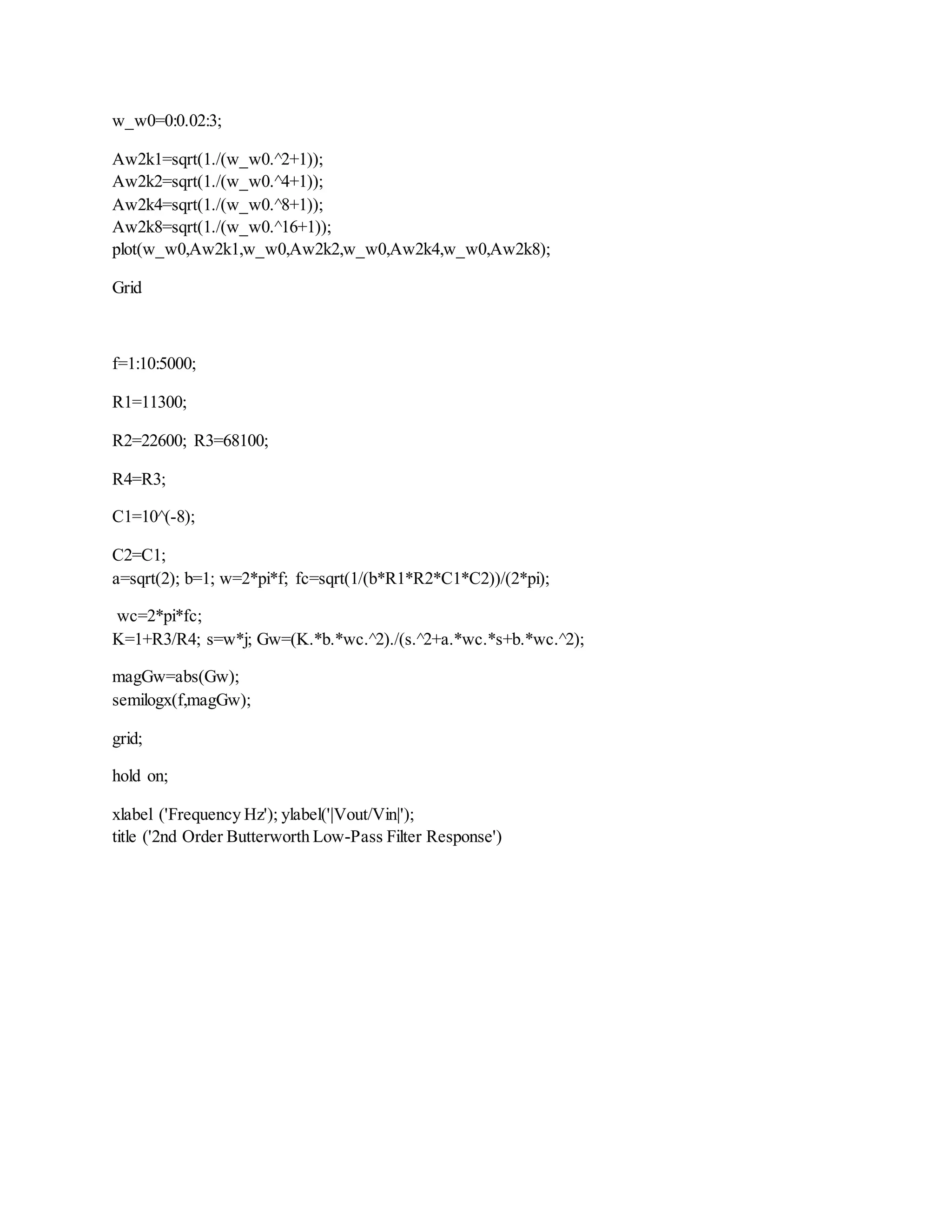
The document contains code for designing and analyzing Butterworth and Chebyshev filters. It includes code to: 1) Design 2nd order Butterworth low-pass and high-pass filters based on filter parameters like cutoff frequency and component values. 2) Plot the magnitude response of the Butterworth filters to visualize the frequency response. 3) Design Butterworth and Chebyshev low-pass filters based on passband and stopband edge frequencies and ripple parameters. 4) Generate and plot the frequency responses of the Butterworth and Chebyshev filters for comparison.

1. w_w0=0:0.02:3;
Aw2k1=sqrt(1./(w_w0.^2+1));
Aw2k2=sqrt(1./(w_w0.^4+1));
Aw2k4=sqrt(1./(w_w0.^8+1));
Aw2k8=sqrt(1./(w_w0.^16+1));
plot(w_w0,Aw2k1,w_w0,Aw2k2,w_w0,Aw2k4,w_w0,Aw2k8);
Grid
f=1:10:5000;
R1=11300;
R2=22600; R3=68100;
R4=R3;
C1=10^(-8);
C2=C1;
a=sqrt(2); b=1; w=2*pi*f; fc=sqrt(1/(b*R1*R2*C1*C2))/(2*pi);
wc=2*pi*fc;
K=1+R3/R4; s=w*j; Gw=(K.*b.*wc.^2)./(s.^2+a.*wc.*s+b.*wc.^2);
magGw=abs(Gw);
semilogx(f,magGw);
grid;
hold on;
xlabel ('Frequency Hz'); ylabel('|Vout/Vin|');
title ('2nd Order Butterworth Low-Pass Filter Response')

2. a=sqrt(2); b =1; C1=10^(-8); C2=C1; fc=1000; wc=2*pi*fc; K=2;
R2=(4*b)/(C1*sqrt(a^2+8*b*(K-1))*wc);
R1=b/(C1^2*R2*wc^2); R3=(K*R2)/(K-1); R4=K*R2; fprintf(' n');
fprintf('R1 = %5.0f Ohms t',R1); fprintf('R2 = %5.0f Ohms t',R2);
fprintf('R3 = %5.0f Ohms t',R3); fprintf('R4 = %5.0f Ohms t',R4)
f=10:10:20000; w=2*pi*f; R1=12700; R2=20000; R3=40200; R4=R3; K=1+R4/R3;
wc=(4*b)/(C1*sqrt(a^2+8*b*(K-1))*R2);
s=w*j;
Gw=(K.*s.^2)./(s.^2+a.*wc.*s./b+wc.^2./b);
semilogx(f,abs(Gw)); grid; hold on;
xlabel('Frequency, Hz'), ylabel('|Vout/Vin|');
title('2nd Order Butterworth High-Pass Filter Response')
fplot('cos(x)',[-2*pi 2*pi -1.2 1.2])
fplot('sin(x)./x',[-20 20 -0.4 1.2])
fplot(@(x)cos(x)), [-2*pi 2*pi -1.2 1.2]
fplot(@(x)sin(x)./x)), [-20 20 -0.4 1.2]
Wp=10; Ws=16.5; r=2;Gs=-20;
[n,Wp]=chebylord (Wp,Ws,r,-Gs, 's');
[num, den]=chebyl (n ,r, Wp, 's' );

3. %%%%%%%%%%%%%%%%%%%
% Example 6.8 -- Filtering with Butterworth filter
%%%%%%%%%%%%%%%%%%%
clear all; clf
syms t w
x = cos(10 * t) - 2 * cos(5 * t) + 4 * sin(20 * t);% input signal
X = fourier(x);
N = 3; Whp = 5; % filter parameters
[b, a] = butter(N, Whp, ’s’); % filter design
W = 0:0.01:30; Hm = abs(freqs(b, a, W)); % magnitude responsein W
% filter output
n = N:-1:0; U = ( j * w).ˆn
num = b - conj(U’); den = a - conj(U’);H = num/den; % frequency response
Y = X * H; % convolution property
y = ifourier(Y, t); % inverse Fourier
%%%%%%%%%%%%%%%%%%%
% Example 6.9 -- Filtering with Butterworth and Chebyshev filters
%%%%%%%%%%%%%%%%%%%
clear all;clf
syms t w
x = cos(10 ∗ t) - 2 ∗ cos(5 ∗ t) + 4 ∗ sin(20 ∗ t); X = fourier(x)
wp = 5;ws = 10;alphamax = 0.1;alphamin = 15; % filter parameters
% butterworth filter
[N, whp] = buttord(wp, ws, alphamax, alphamin, ’s’)
[b, a] = butter(N, whp, ’s’)
% cheby1 filter
epsi= sqrt(10ˆ(alphamax/10) -1)
wp = whp/cosh(acosh(1/epsi)/N) % recomputing wp to get same whp
[N1, wn] = cheb1ord(wp, ws, alphamax, alphamin, ’s’);
[b1, a1] = cheby1(N1, alphamax, wn, ’s’);
% frequency responses
W = 0:0.01:30;
Hm = abs(freqs(b, a, W));
Hm1 = abs(freqs(b1, a1, W));
% generation of frequency responsefrom coefficients
n = N:-1:0; n1 = N1:-1:0;
U = ( j * w).^n; U1 = ( j *w).^n1
num = b .*conj(U’); den = a .* conj(U’);
num1 = b1 conj(U1’); den1 = a1 ∗ conj(U1’)
H = num/den; % Butterworth LPF
H1 = num1/den1; % Chebyshev LPF
% output of filter
Y = X ∗ H;
Y1 = X ∗ H1;
y = ifourier(Y, t)
y1 = ifourier(Y1, t