process control

1. Process Control and
Capability
Prakash Awasthy

2. TQM review
• Highlight the problem
• Identify opportunity [Histograms, Pareto diagram]
• Analyze problem [Fishbone, CEDAC]
• Operational planning [Poka yoke]
“Quality in a service or product is not what you put into it. It is what the client or
customer gets out of it”
-Peter Drucker

3. Process Variability
• It’s everywhere
• What is process variability?
• Dimensions
• Causes

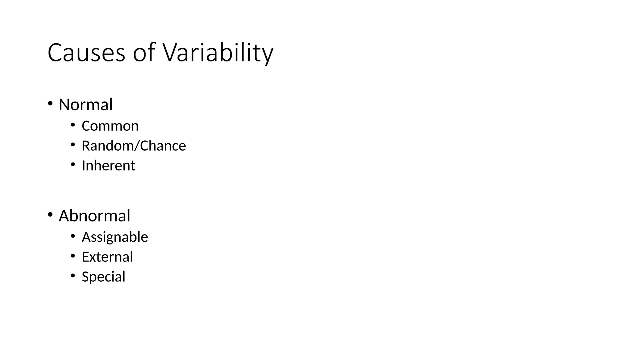
4. Causes of Variability
• Normal
• Common
• Random/Chance
• Inherent
• Abnormal
• Assignable
• External
• Special

5. Process Control
• The goal of process control is to identify if the variability is assignable
or random
• And, take appropriate action
• How to identify?
• Control charts

6. Control chart
• If variability is too much (beyond a band), it could be due to
assignable reasons
• Statistical Process Control (SPC) involves establishing a control band of
acceptable variation in the process performance
• Control band  [LCL, UCL]

7. Let’s watch a video

8. Measures in control charts
• Mean,
• Range, R
• Proportion of defects, p
• Number of defects, c

9. 𝑋 h
𝐶 𝑎𝑟𝑡
• Process average (centre line),
• UCL =
• LCL =
Sample
size (n)
2 1.880 0 3.268
3 1.023 0 2.574
4 0.729 0 2.282
5 0.577 0 2.114
6 0.483 0 2.004
7 0.419 0.076 1.924
8 0.373 0.136 1.864
9 0.337 0.184 1.816
10 0.308 0.223 1.777
Control chart constants

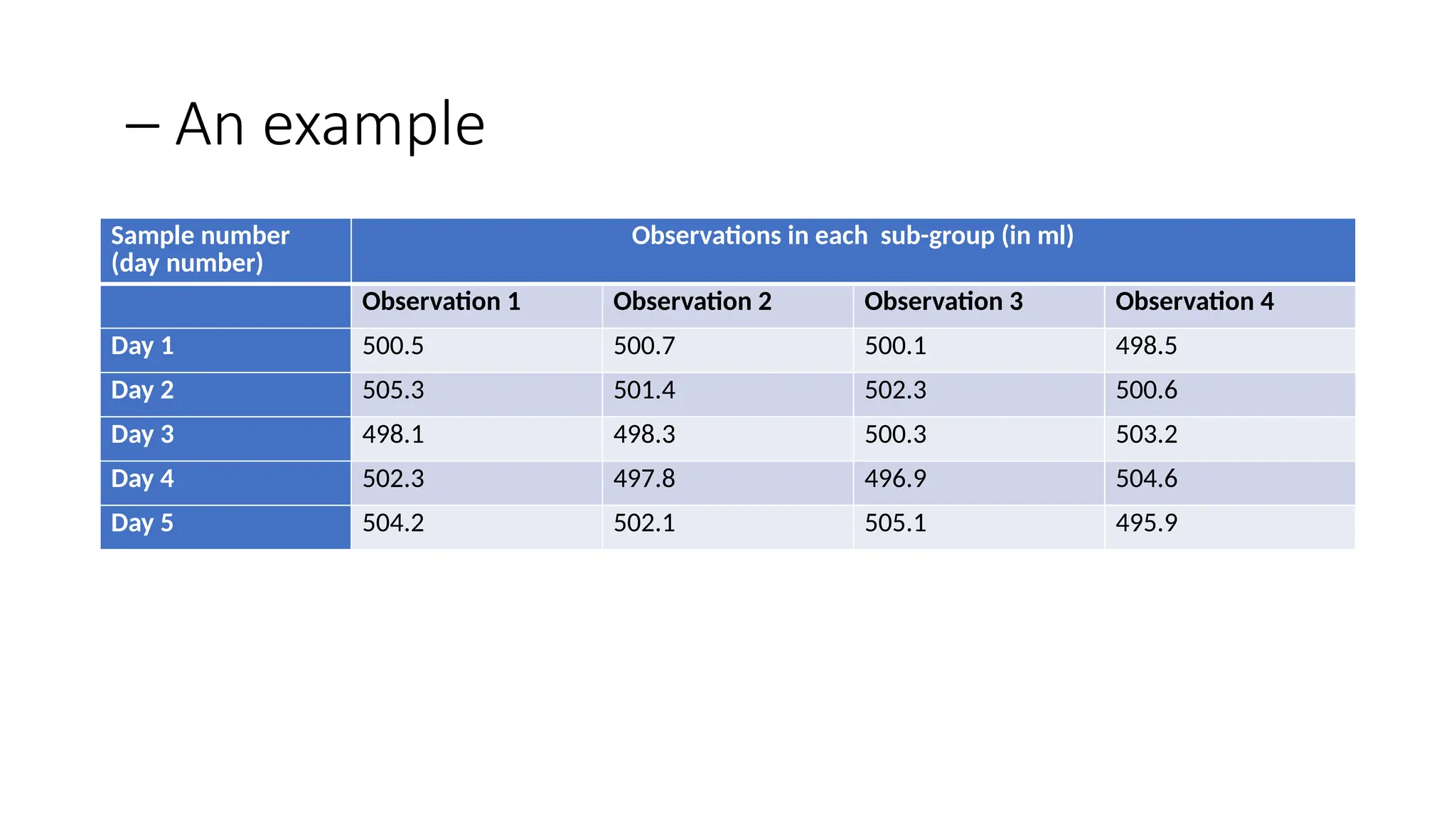
10. – An example
Sample number
(day number)
Observations in each sub-group (in ml)
Observation 1 Observation 2 Observation 3 Observation 4
Day 1 500.5 500.7 500.1 498.5
Day 2 505.3 501.4 502.3 500.6
Day 3 498.1 498.3 500.3 503.2
Day 4 502.3 497.8 496.9 504.6
Day 5 504.2 502.1 505.1 495.9

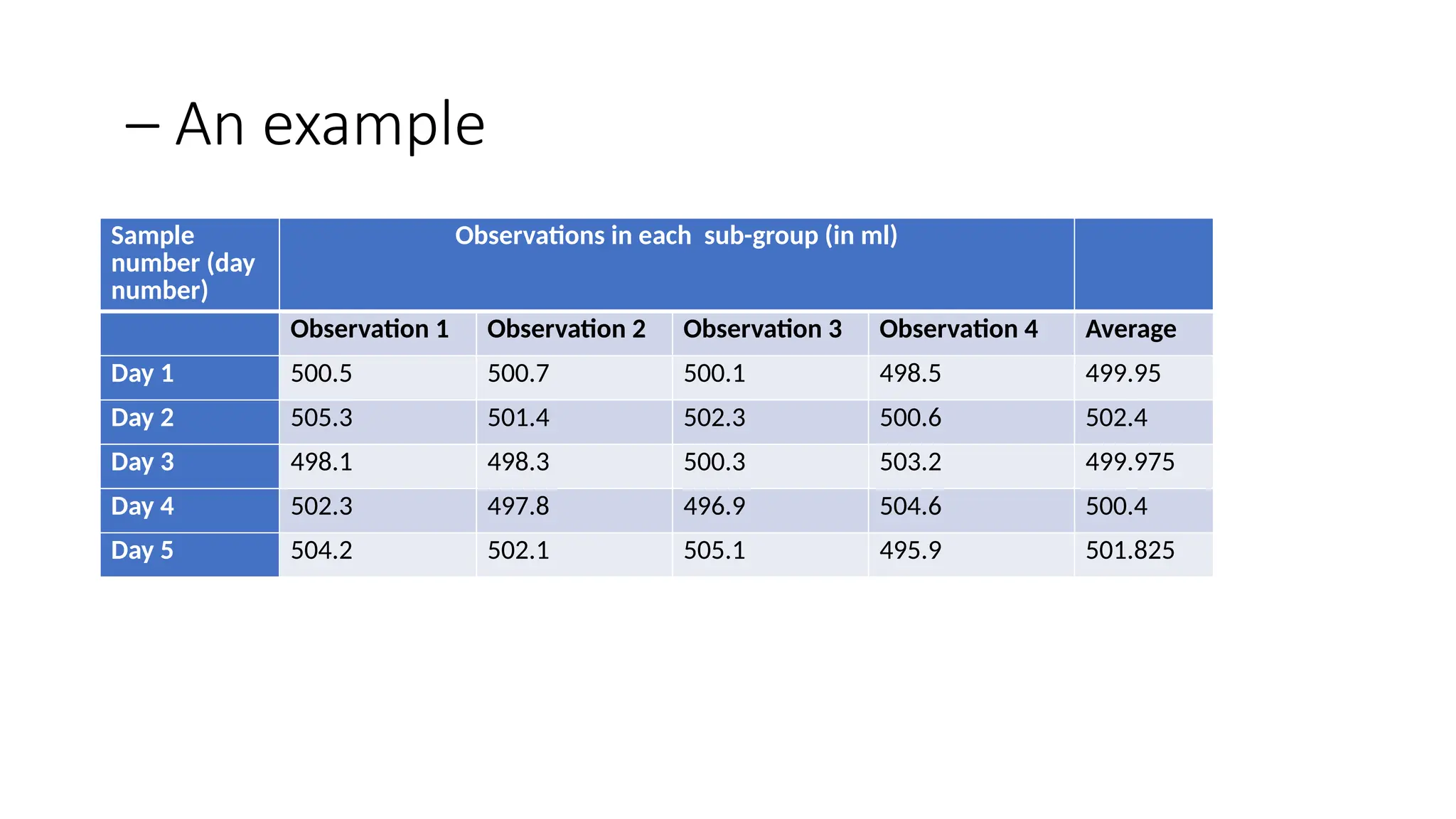
11. – An example
Sample
number (day
number)
Observations in each sub-group (in ml)
Observation 1 Observation 2 Observation 3 Observation 4 Average
Day 1 500.5 500.7 500.1 498.5 499.95
Day 2 505.3 501.4 502.3 500.6 502.4
Day 3 498.1 498.3 500.3 503.2 499.975
Day 4 502.3 497.8 496.9 504.6 500.4
Day 5 504.2 502.1 505.1 495.9 501.825

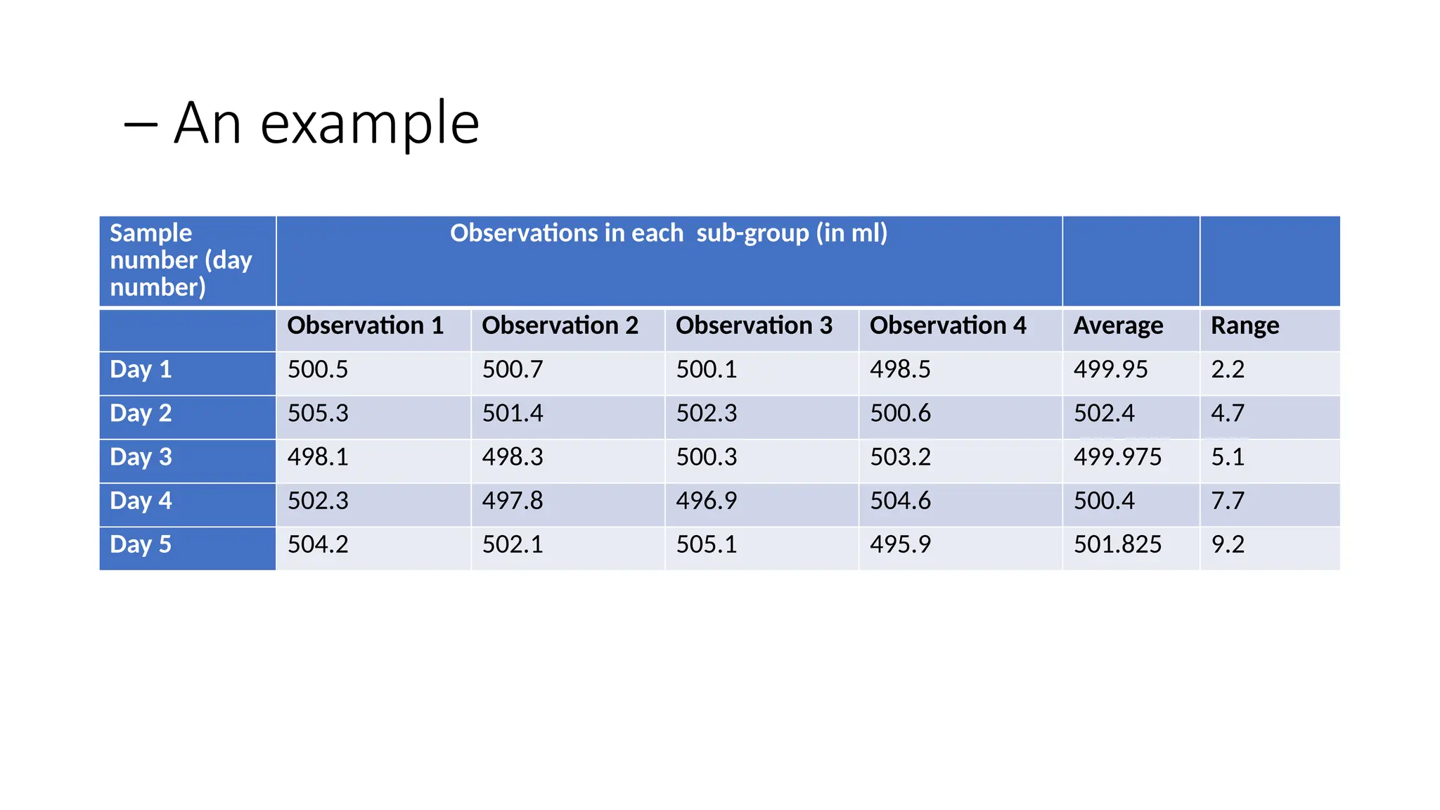
12. – An example
Sample
number (day
number)
Observations in each sub-group (in ml)
Observation 1 Observation 2 Observation 3 Observation 4 Average Range
Day 1 500.5 500.7 500.1 498.5 499.95 2.2
Day 2 505.3 501.4 502.3 500.6 502.4 4.7
Day 3 498.1 498.3 500.3 503.2 499.975 5.1
Day 4 502.3 497.8 496.9 504.6 500.4 7.7
Day 5 504.2 502.1 505.1 495.9 501.825 9.2

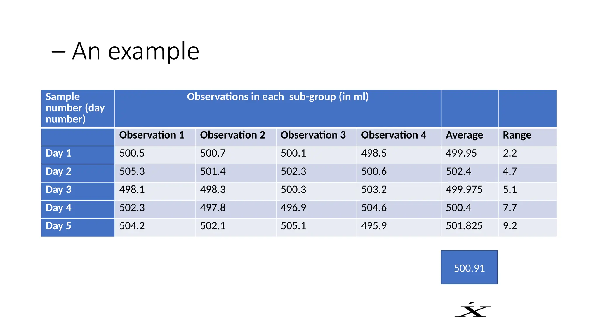
13. – An example
Sample
number (day
number)
Observations in each sub-group (in ml)
Observation 1 Observation 2 Observation 3 Observation 4 Average Range
Day 1 500.5 500.7 500.1 498.5 499.95 2.2
Day 2 505.3 501.4 502.3 500.6 502.4 4.7
Day 3 498.1 498.3 500.3 503.2 499.975 5.1
Day 4 502.3 497.8 496.9 504.6 500.4 7.7
Day 5 504.2 502.1 505.1 495.9 501.825 9.2
500.91
´
𝑋

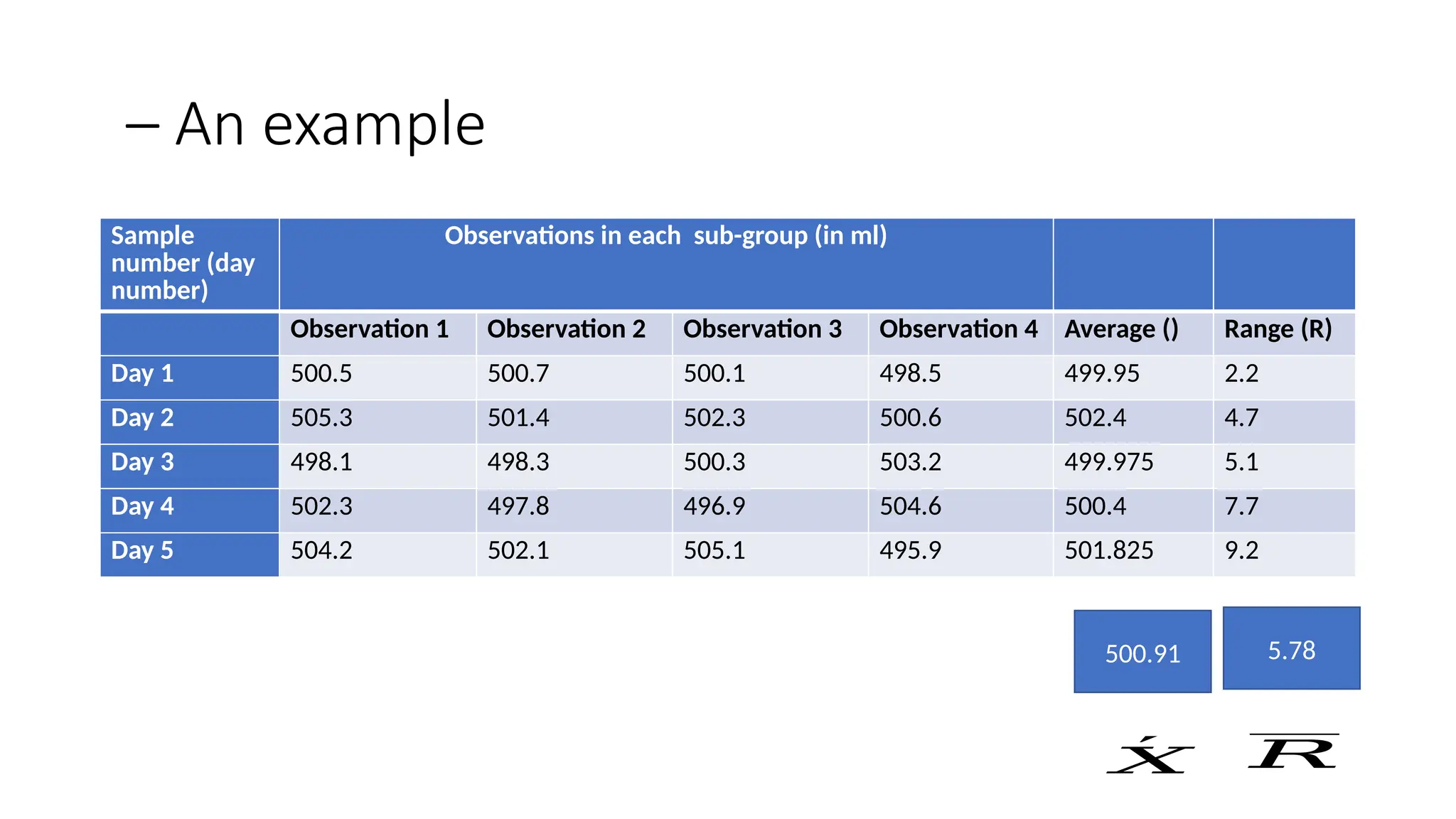
14. – An example
Sample
number (day
number)
Observations in each sub-group (in ml)
Observation 1 Observation 2 Observation 3 Observation 4 Average () Range (R)
Day 1 500.5 500.7 500.1 498.5 499.95 2.2
Day 2 505.3 501.4 502.3 500.6 502.4 4.7
Day 3 498.1 498.3 500.3 503.2 499.975 5.1
Day 4 502.3 497.8 496.9 504.6 500.4 7.7
Day 5 504.2 502.1 505.1 495.9 501.825 9.2
500.91
´
𝑋
5.78
𝑅

15. – An example
Sample
number (day
number)
Observations in each sub-group (in ml)
Observation 1 Observation 2 Observation 3 Observation 4 Average () Range (R)
Day 1 500.5 500.7 500.1 498.5 499.95 2.2
Day 2 505.3 501.4 502.3 500.6 502.4 4.7
Day 3 498.1 498.3 500.3 503.2 499.975 5.1
Day 4 502.3 497.8 496.9 504.6 500.4 7.7
Day 5 504.2 502.1 505.1 495.9 501.825 9.2
500.91
´
𝑋
5.78
𝑅
UCL =
LCL = = 500.91 – 0.729*5.78 = 496.6964

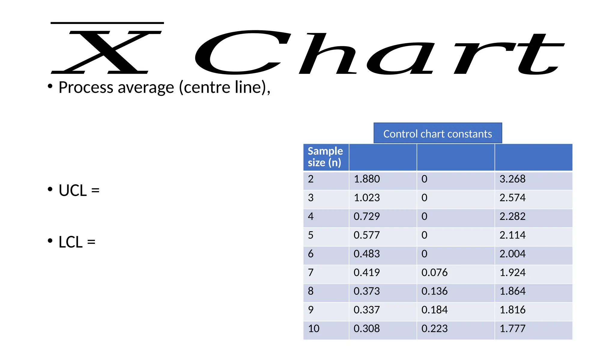
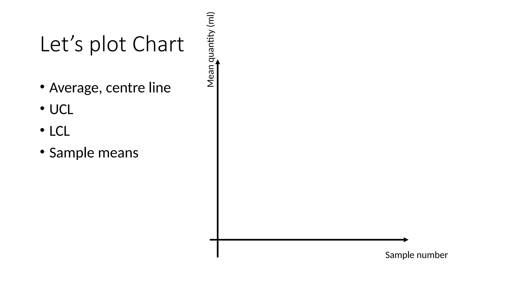
16. Let’s plot Chart
• Average, centre line
• UCL
• LCL
• Sample means
Sample number
Mean
quantity
(ml)

17. 𝑅 h
𝐶 𝑎𝑟𝑡
• Process average, centre line
• UCL =
• LCL =

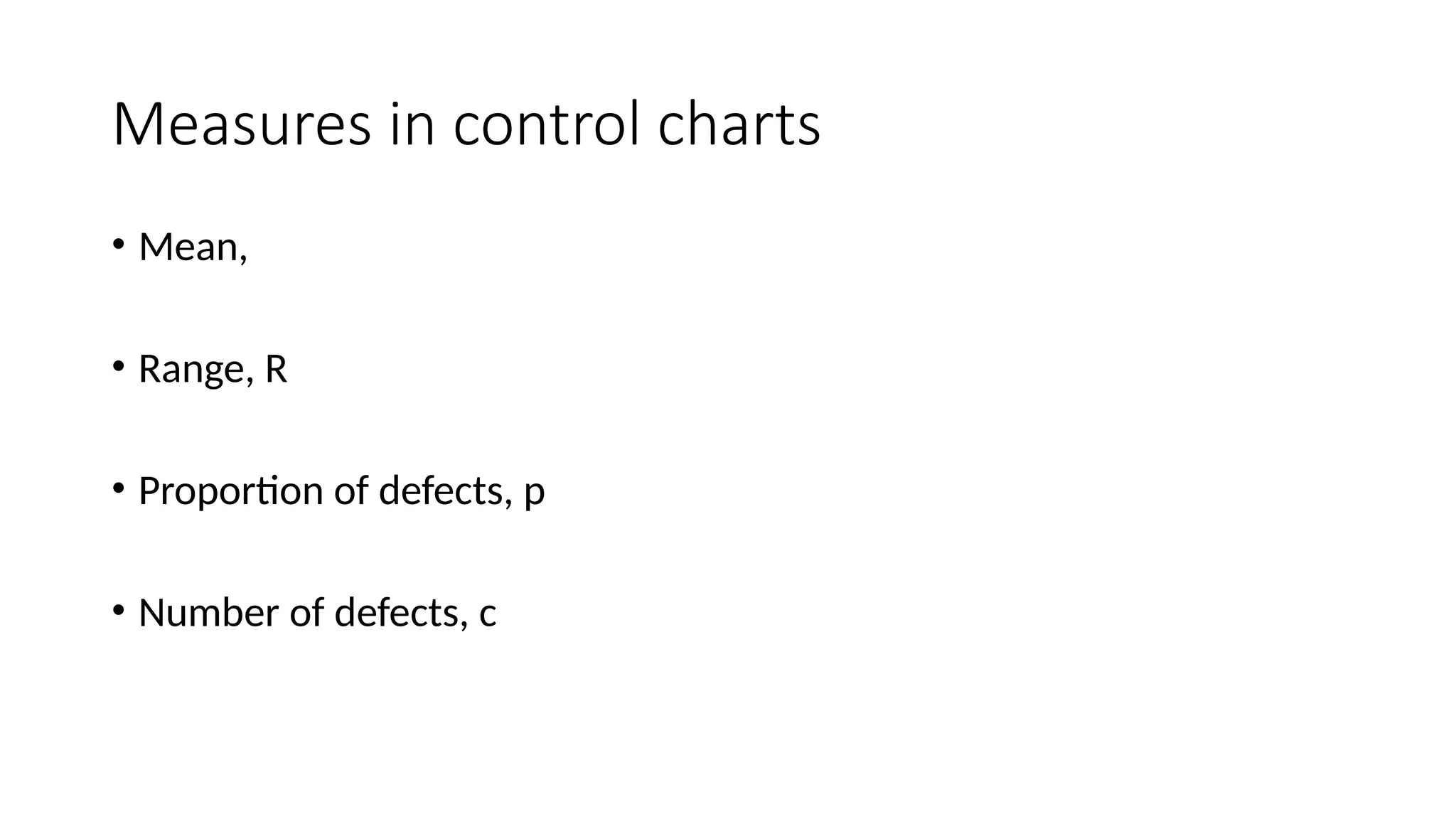
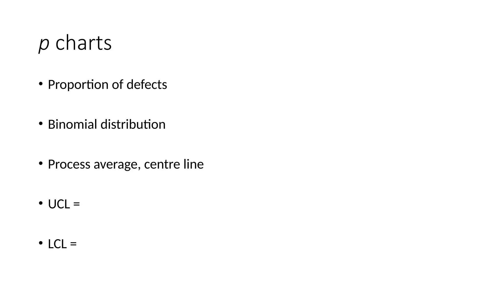
18. p charts
• Proportion of defects
• Binomial distribution
• Process average, centre line
• UCL =
• LCL =

19. c charts
• Number of defects
• Process average, centre line
• UCL =
• LCL =

20. Process Capability

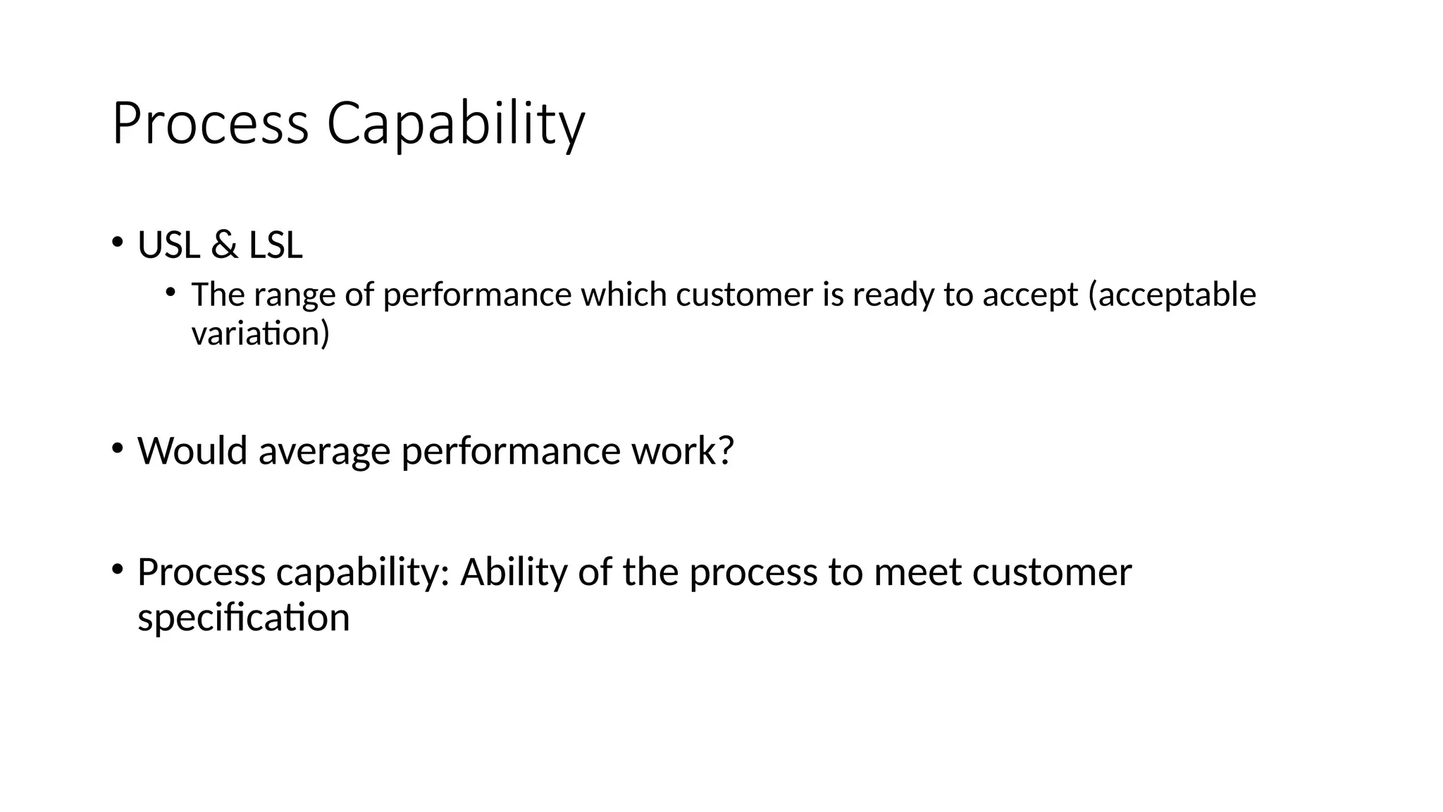
21. Process Capability
• USL & LSL
• The range of performance which customer is ready to accept (acceptable
variation)
• Would average performance work?
• Process capability: Ability of the process to meet customer
specification

22. Potential capability
Process capability and Proportion defective
Defects (ppm) 10,000 3,000 1,000 100 10 1 2ppb
0.86 1 1.1 1.3 1.47 1.63 2

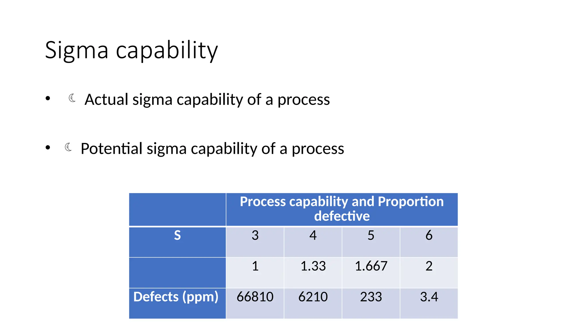
23. Sigma capability
•  Actual sigma capability of a process
•  Potential sigma capability of a process
Process capability and Proportion
defective
S 3 4 5 6
1 1.33 1.667 2
Defects (ppm) 66810 6210 233 3.4

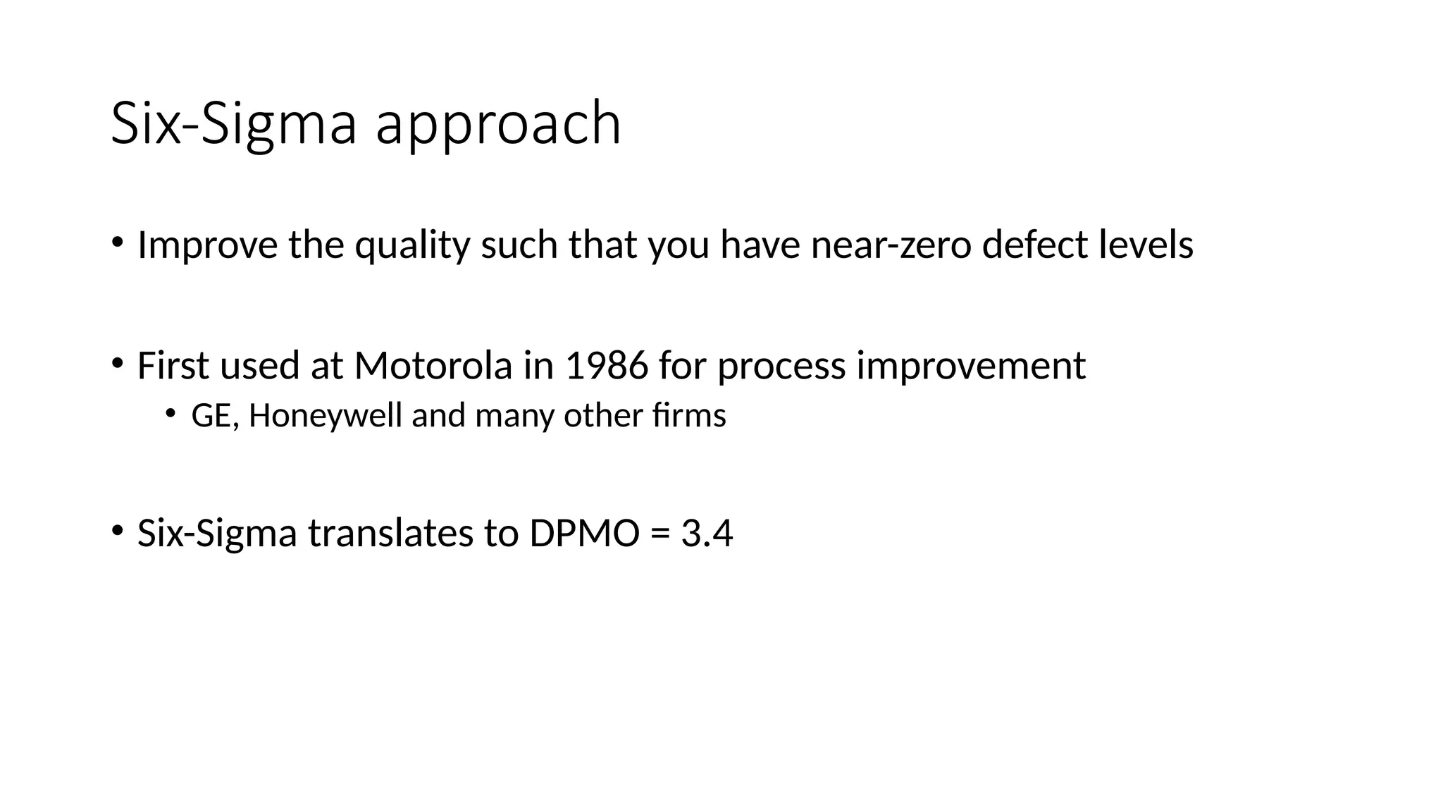
24. Six-Sigma approach
• Improve the quality such that you have near-zero defect levels
• First used at Motorola in 1986 for process improvement
• GE, Honeywell and many other firms
• Six-Sigma translates to DPMO = 3.4

25. Six-Sigma methodology
• DMAIC
• Define
• Measure
• Analyze
• Improve
• Control

26. Define
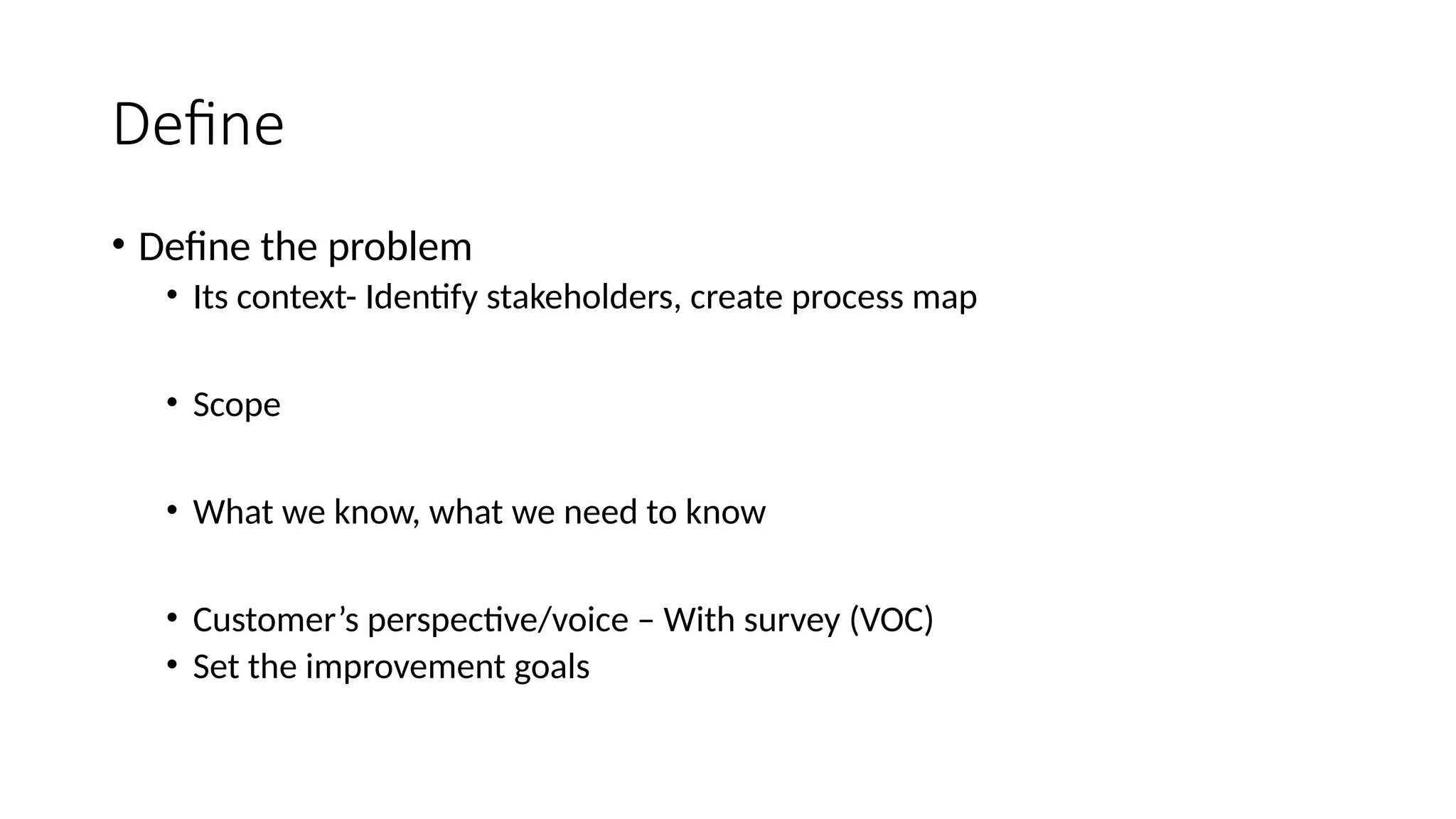
• Define the problem
• Its context- Identify stakeholders, create process map
• Scope
• What we know, what we need to know
• Customer’s perspective/voice – With survey (VOC)
• Set the improvement goals

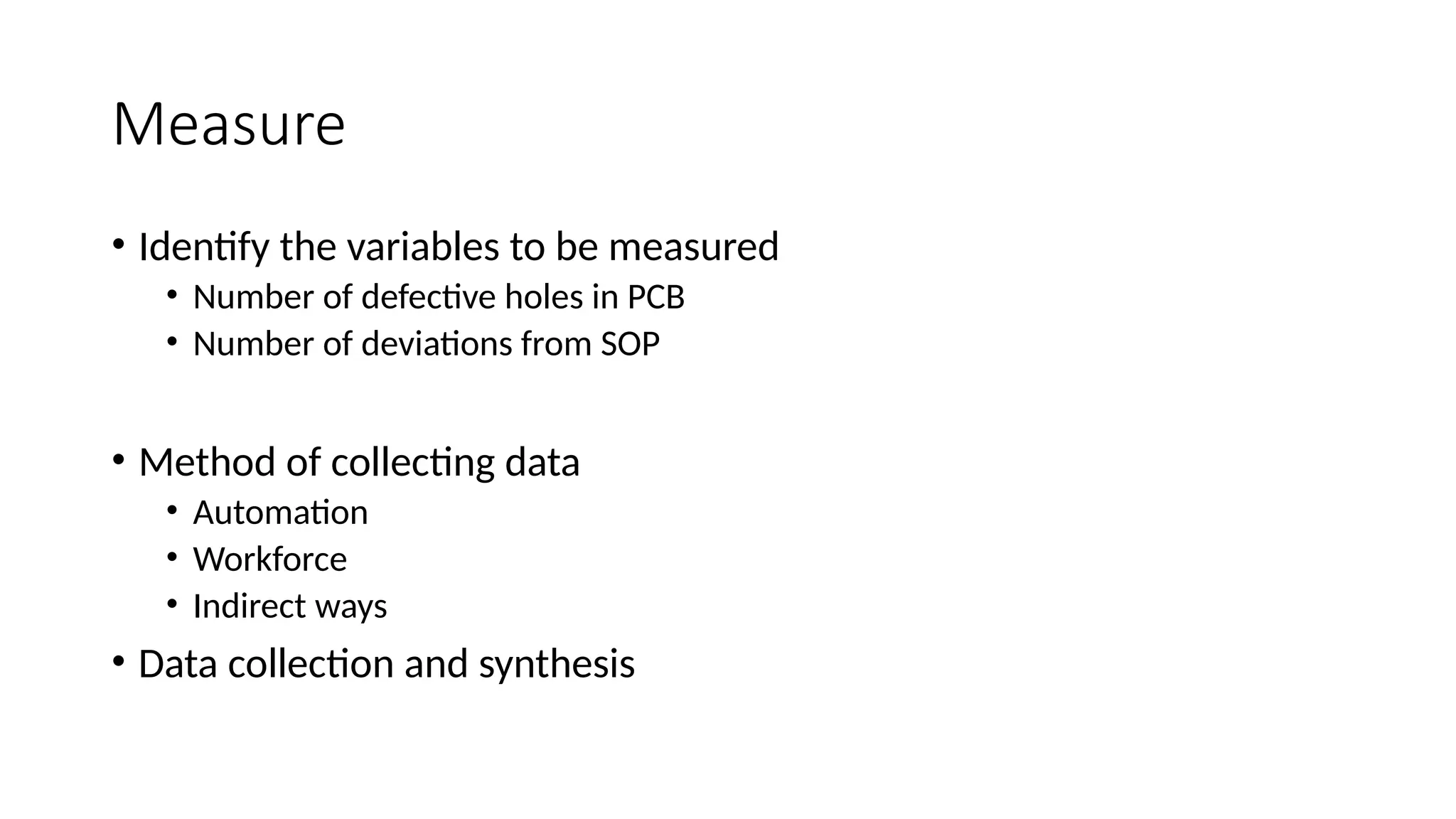
27. Measure
• Identify the variables to be measured
• Number of defective holes in PCB
• Number of deviations from SOP
• Method of collecting data
• Automation
• Workforce
• Indirect ways
• Data collection and synthesis

28. Analyze
• Possible causes of bad quality
• Identify areas to reduce defects
• Develop and apply tools for analysis
• Graphs, charts
• Identify possible source of variation
• How can we eliminate causes of variation?

29. Analyze
• Sharpness causing variability
• The sharpness of cutting tool changes with time and temperature
• Hardness causing variability
• Hardness of bread changes with moisture, texture

30. Improve
• Elimination of root causes of variability
• Generating and validating improvement alternatives
• Create new process map or SOP
• About frequent sharpening or moisture control

31. Control
• Ensure that process follows new plan/standard
• Develop control plan
• Organize training for new plan
• Establish new plan as a standard