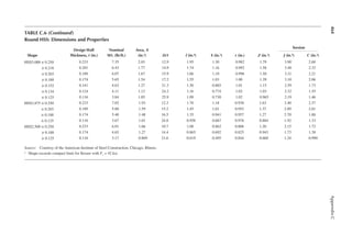
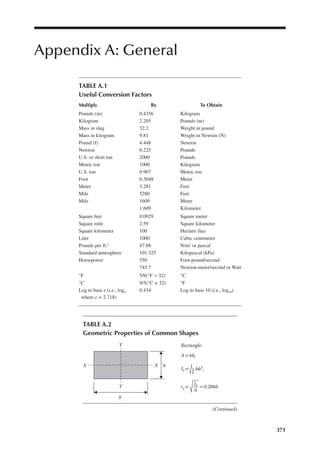
This document provides an overview and table of contents for the book "Principles of Structural Design: Wood, Steel, and Concrete" by Ram S. Gupta. The book covers design principles and loads for wood, steel, and reinforced concrete structures over four sections. It includes chapters on design loads such as dead loads, live loads, snow loads, and wind loads. It also covers analysis and design of structural elements for each material such as beams, columns, slabs, connections, and combined forces.

3. Principles of
STRUCTURAL
DESIGN
Wood, Steel, and Concrete
SECOND EDITION

5. Boca Raton London New York
CRC Press is an imprint of the
Taylor & Francis Group, an informa business
Principles of
STRUCTURAL
DESIGN
Wood, Steel, and Concrete
SECOND EDITION
RAM S. GUPTA

6. CRC Press
Taylor & Francis Group
6000 Broken Sound Parkway NW, Suite 300
Boca Raton, FL 33487-2742
© 2014 by Taylor & Francis Group, LLC
CRC Press is an imprint of Taylor & Francis Group, an Informa business
No claim to original U.S. Government works
Version Date: 20140213
International Standard Book Number-13: 978-1-4665-5233-3 (eBook - PDF)
This book contains information obtained from authentic and highly regarded sources. Reasonable efforts have been
made to publish reliable data and information, but the author and publisher cannot assume responsibility for the valid-
ity of all materials or the consequences of their use. The authors and publishers have attempted to trace the copyright
holders of all material reproduced in this publication and apologize to copyright holders if permission to publish in this
form has not been obtained. If any copyright material has not been acknowledged please write and let us know so we may
rectify in any future reprint.
Except as permitted under U.S. Copyright Law, no part of this book may be reprinted, reproduced, transmitted, or uti-
lized in any form by any electronic, mechanical, or other means, now known or hereafter invented, including photocopy-
ing, microfilming, and recording, or in any information storage or retrieval system, without written permission from the
publishers.
For permission to photocopy or use material electronically from this work, please access www.copyright.com (http://
www.copyright.com/) or contact the Copyright Clearance Center, Inc. (CCC), 222 Rosewood Drive, Danvers, MA 01923,
978-750-8400. CCC is a not-for-profit organization that provides licenses and registration for a variety of users. For
organizations that have been granted a photocopy license by the CCC, a separate system of payment has been arranged.
Trademark Notice: Product or corporate names may be trademarks or registered trademarks, and are used only for
identification and explanation without intent to infringe.
Visit the Taylor & Francis Web site at
http://www.taylorandfrancis.com
and the CRC Press Web site at
http://www.crcpress.com

7. v
Contents
Preface............................................................................................................................................ xiii
Author ..............................................................................................................................................xv
Section i Design Loads
Chapter 1 Design Criteria .............................................................................................................3
Classiication of Buildings ...........................................................................................3
Building Codes.............................................................................................................3
Standard Unit Loads.....................................................................................................3
Tributary Area..............................................................................................................3
Working Stress Design, Strength Design, and Uniied Design of Structures..............7
Elastic and Plastic Designs.........................................................................................10
Elastic Moment Capacity.......................................................................................12
Plastic Moment Capacity.......................................................................................12
Combinations of Loads .............................................................................................. 14
Other Loads................................................................................................................15
Continuous Load Path for Structural Integrity .......................................................... 18
Problems..................................................................................................................... 18
Chapter 2 Primary Loads: Dead Loads and Live Loads ............................................................23
Dead Loads.................................................................................................................23
Live Loads..................................................................................................................24
Floor Live Loads ........................................................................................................24
Basic Design Live Load, Lo...................................................................................24
Effective Area Reduction Factor ...........................................................................24
Other Provisions for Floor Live Loads.......................................................................26
Multiple Floors Reductions ...................................................................................27
Roof Live Loads, Lr....................................................................................................28
Tributary Area Reduction Factor, R1 .....................................................................28
Slope Reduction Factor..........................................................................................28
Problems.....................................................................................................................29
Chapter 3 Snow Loads ................................................................................................................ 31
Introduction................................................................................................................ 31
Minimum Snow Load for Low-Slope Roofs.............................................................. 31
Balanced Snow Load..................................................................................................34
Importance Factor .................................................................................................34
Thermal Factor, Ct.................................................................................................34
Exposure Factor, Ce ...............................................................................................35
Roof Slope Factor, Cs.............................................................................................35

8. vi Contents
Rain-on-Snow Surcharge ...........................................................................................36
Partial Loading of the Balanced Snow Load .............................................................37
Unbalanced across the Ridge Snow Load..................................................................38
Snow Drift from a Higher to a Lower Roof...............................................................40
Leeward Snow Drift on Lower Roof of Attached Structure.................................40
Windward Snow Drift on Lower Roof of Attached Structure .............................. 41
Leeward Snow Drift on Lower Roof of Separated Structure................................42
Windward Snow Drift on Lower Roof of Separated Structure.............................42
Sliding Snow Load on Lower Roof............................................................................44
Sliding Snow Load on Separated Structures..............................................................46
Problems.....................................................................................................................46
Chapter 4 Wind Loads ................................................................................................................49
Introduction................................................................................................................49
Deinition of Terms ....................................................................................................49
Procedures for MWFRS.............................................................................................50
Simpliied Procedure for MWFRS for Low-Rise Buildings......................................50
Horizontal Pressure Zones for MWFRS...............................................................57
Vertical Pressure Zones for MWFRS ................................................................... 61
Minimum Pressure for MWFRS........................................................................... 61
Procedures for Components and Cladding.................................................................66
Simpliied Procedure for Components and Cladding for
Low-Rise Buildings....................................................................................................66
Minimum Pressures for Components and Cladding .............................................70
Problems.....................................................................................................................72
Chapter 5 Earthquake Loads ......................................................................................................75
Seismic Forces............................................................................................................75
Seismic Design Procedures........................................................................................75
Deinitions..................................................................................................................76
Structural Height ...................................................................................................76
Stories above Base and Grade Plane .....................................................................76
Fundamental Period of Structure ..........................................................................77
Ground Motion Response Accelerations....................................................................77
Mapped MCER Spectral Response Acceleration Parameters................................78
Adjustments to Spectral Response Acceleration Parameters for Site
Class Effects..........................................................................................................78
Design Spectral Acceleration Parameters .............................................................78
Design Response Spectrum...................................................................................78
Importance Factor, I...................................................................................................88
Seismic Design Categories.........................................................................................88
Exemptions from Seismic Designs.............................................................................90
Equivalent Lateral Force Procedure to Determine Seismic Force.............................90
Effective Weight of Structure, W...........................................................................90
Seismic Response Coeficient, Cs..........................................................................90
Response Modiication Factor or Coeficient, R.................................................... 91
Distribution of Seismic Forces...................................................................................92
Distribution of Seismic Forces on Vertical Wall Elements...................................92
Distribution of Seismic Forces on Horizontal
Elements (Diaphragms).........................................................................................93

9. vii
Contents
Design Earthquake Load............................................................................................94
Soil–Structure Interaction..........................................................................................98
Problems.....................................................................................................................99
Section ii Wood Structures
Chapter 6 Wood Speciications................................................................................................. 105
Engineering Properties of Sawn Lumber................................................................. 105
Reference Design Values for Sawn Lumber............................................................. 105
Adjustments to the Reference Design Values for Sawn Lumber..............................106
Time Effect Factor, λ...........................................................................................107
Size Factor, CF .....................................................................................................107
Size Factor, CF, for Dimension Lumber..........................................................108
Size Factor, CF, for Timber.............................................................................108
Repetitive Member Factor, Cr..............................................................................108
Flat Use Factor, Cfu ..............................................................................................108
Buckling Stiffness Factor, CT ..............................................................................108
Bearing Area Factor, Cb ......................................................................................108
Format Conversion Factor, KF .............................................................................109
Resistance Factor, ϕ.............................................................................................109
Load Resistance Factor Design with Wood .............................................................109
Structural Glued Laminated Timber........................................................................ 114
Reference Design Values for Glued Laminated Timber .......................................... 115
Adjustment Factors for Glued Laminated Timber ................................................... 116
Flat Use Factor for Glued Laminated Timber, CFU ............................................. 116
Volume Factor for Glued Laminated Timber, Cv ................................................ 116
Curvature Factor for Glued Laminated Timber, Cc ............................................ 116
Stress Interaction Factor, CI................................................................................. 118
Shear Reduction Factor, CVR................................................................................ 118
Structural Composite Lumber..................................................................................120
Summary of Adjustment Factors.............................................................................. 121
Problems...................................................................................................................123
Chapter 7 Flexure and Axially Loaded Wood Structures ........................................................125
Introduction..............................................................................................................125
Design of Beams ......................................................................................................125
Bending Criteria of Design ......................................................................................125
Beam Stability Factor, CL.........................................................................................127
Effective Unbraced Length..................................................................................128
Shear Criteria ...........................................................................................................129
Delection Criteria.................................................................................................... 131
Creep Delection....................................................................................................... 132
Bearing at Supports..................................................................................................136
Bearing Area Factor, Cb ...................................................................................... 137
Design of Axial Tension Members...........................................................................138
Design of Columns................................................................................................... 140
Column Stability Factor, CP ..................................................................................... 141
Design for Combined Bending and Compression.................................................... 143
Problems................................................................................................................... 147

10. viii Contents
Chapter 8 Wood Connections ................................................................................................... 153
Types of Connections and Fasteners ........................................................................ 153
Dowel-Type Fasteners (Nails, Screws, Bolts, Pins).................................................. 153
Yield Limit Theory for Laterally Loaded Fasteners................................................154
Yield Mechanisms and Yield Limit Equations ........................................................ 155
Reference Design Values for Lateral Loads (Shear Connections) ........................... 157
Reference Design Values for Withdrawal Loads ..................................................... 157
Adjustments of the Reference Design Values .......................................................... 157
Wet Service Factor, CM........................................................................................ 158
Temperature Factor, Ct ........................................................................................ 158
Group Action Factor, Cg ...................................................................................... 158
Geometry Factor, C∆............................................................................................ 158
End Grain Factor, Ceg .......................................................................................... 161
Diaphragm Factor, Cdi ......................................................................................... 161
Toenail Factor, Ctn ............................................................................................... 161
Nail and Screw Connections....................................................................................164
Common, Box, and Sinker Nails.........................................................................164
Post-Frame Ring Shank Nails .............................................................................164
Wood Screws....................................................................................................... 165
Bolt and Lag Screw Connections............................................................................. 166
Bolts..................................................................................................................... 167
Lag Screws .......................................................................................................... 167
Problems................................................................................................................... 168
Section iii Steel Structures
Chapter 9 Tension Steel Members ............................................................................................ 175
Properties of Steel .................................................................................................... 175
Provisions to Design Steel Structures ...................................................................... 175
Uniied Design Speciications.................................................................................. 176
Limit States of Design......................................................................................... 176
Design of Tension Members..................................................................................... 177
Tensile Strength of Elements.................................................................................... 177
Net Area, An......................................................................................................... 178
Effective Net Area, Ae ......................................................................................... 179
Block Shear Strength................................................................................................ 182
Design Procedure for Tension Members.................................................................. 184
Problems................................................................................................................... 186
Chapter 10 Compression Steel Members.................................................................................... 191
Strength of Compression Members or Columns...................................................... 191
Local Buckling Criteria............................................................................................ 193
Flexural Buckling Criteria .......................................................................................194
Effective Length Factor for Slenderness Ratio ........................................................194
Limit States for Compression Design ......................................................................197
Nonslender Members................................................................................................197
Flexural Buckling of Nonslender Members in Elastic and
Inelastic Regions..................................................................................................197

11. ix
Contents
Inelastic Buckling................................................................................................ 198
Elastic Buckling................................................................................................... 198
Torsional and Flexural–Torsional Buckling of Nonslender
Members.............................................................................................................. 198
Single-Angle Members.............................................................................................200
Built-Up Members....................................................................................................200
Slender Compression Members................................................................................200
Use of the Compression Tables ................................................................................200
Problems...................................................................................................................203
Chapter 11 Flexural Steel Members ...........................................................................................209
Basis of Design.........................................................................................................209
Nominal Strength of Steel in Flexure ......................................................................209
Lateral Unsupported Length ....................................................................................209
Fully Plastic Zone with Adequate Lateral Support.................................................. 211
Inelastic Lateral Torsional Buckling Zone............................................................... 211
Modiication Factor Cb ............................................................................................. 211
Elastic Lateral Torsional Buckling Zone.................................................................. 212
Noncompact and Slender Beam Sections for Flexure.............................................. 212
Compact Full Plastic Limit ...................................................................................... 213
Noncompact Flange Local Buckling........................................................................ 213
Slender Flange Local Buckling................................................................................ 214
Summary of Beam Relations ................................................................................... 214
Design Aids.............................................................................................................. 215
Shear Strength of Steel............................................................................................. 218
Beam Delection Limitations ...................................................................................220
Problems...................................................................................................................222
Chapter 12 Combined Forces on Steel Members........................................................................225
Design Approach to Combined Forces ....................................................................225
Combination of Tensile and Flexure Forces.............................................................225
Combination of Compression and Flexure Forces: The
Beam-Column Members..........................................................................................227
Members without Sidesway.................................................................................227
Members with Sidesway......................................................................................227
Magniication Factor B1.......................................................................................229
Moment Modiication Factor, CM ........................................................................229
K Values for Braced Frames................................................................................ 231
Braced Frame Design............................................................................................... 231
Magniication Factor for Sway, B2............................................................................235
K Values for Unbraced Frames ................................................................................235
Unbraced Frame Design...........................................................................................237
Open-Web Steel Joists..............................................................................................240
Joist Girders..............................................................................................................243
Problems...................................................................................................................245
Chapter 13 Steel Connections..................................................................................................... 251
Types of Connections and Joints.............................................................................. 251
Bolted Connections .................................................................................................. 251

12. x Contents
Speciications for Spacing of Bolts and Edge Distance ...........................................254
Bearing-Type Connections.......................................................................................255
Slip-Critical Connections.........................................................................................259
Tensile Load on Bolts............................................................................................... 261
Combined Shear and Tensile Forces on Bolts..........................................................263
Combined Shear and Tension on Bearing-Type Connections.............................263
Combined Shear and Tension on Slip-Critical Connections...............................265
Welded Connections.................................................................................................267
Groove Welds ...........................................................................................................267
Effective Area of Groove Weld ...........................................................................267
Fillet Welds...............................................................................................................267
Effective Area of Fillet Weld...............................................................................267
Minimum Size of Fillet Weld..............................................................................267
Maximum Size of Fillet Weld .............................................................................268
Length of Fillet Weld...........................................................................................268
Strength of Weld.......................................................................................................268
Complete Joint Penetration Groove Welds..........................................................268
Partial Joint Penetration Welds and Fillet Welds ................................................268
Frame Connections................................................................................................... 271
Shear or Simple Connection for Frames ..................................................................272
Single-Plate Shear Connection or Shear Tab ......................................................272
Framed-Beam Connection...................................................................................272
Seated-Beam Connection ....................................................................................272
End-Plate Connection..........................................................................................272
Single-Plate Shear Connection for Frames .............................................................. 274
Moment-Resisting Connection for Frames ..............................................................277
Problems...................................................................................................................279
Section iV Reinforced concrete Structures
Chapter 14 Flexural Reinforced Concrete Members..................................................................289
Properties of Reinforced Concrete...........................................................................289
Compression Strength of Concrete...........................................................................289
Design Strength of Concrete ....................................................................................290
Strength of Reinforcing Steel................................................................................... 291
Load Resistance Factor Design Basis of Concrete................................................... 291
Reinforced Concrete Beams.....................................................................................292
Derivation of the Beam Relations ............................................................................292
Strain Diagram and Modes of Failure......................................................................294
Balanced and Recommended Steel Percentages......................................................295
Minimum Percentage of Steel..................................................................................295
Strength Reduction Factor for Concrete...................................................................296
Speciications for Beams..........................................................................................296
Analysis of Beams....................................................................................................297
Design of Beams ......................................................................................................299
Design for Reinforcement Only...........................................................................299
Design of Beam Section and Reinforcement.......................................................300

13. xi
Contents
One-Way Slab...........................................................................................................303
Speciications for Slabs ............................................................................................303
Analysis of One-Way Slab........................................................................................304
Design of One-Way Slab ..........................................................................................305
Problems...................................................................................................................306
Chapter 15 Doubly and T Reinforced Concrete Beams.............................................................. 311
Doubly Reinforced Concrete Beams........................................................................ 311
Analysis of Doubly Reinforced Beams.................................................................... 313
Design of Doubly Reinforced Beams....................................................................... 316
Monolithic Slab and Beam (T Beams)..................................................................... 317
Analysis of T Beams ................................................................................................ 318
Design of T Beams...................................................................................................320
Problems...................................................................................................................323
Chapter 16 Shear and Torsion in Reinforced Concrete ..............................................................327
Stress Distribution in Beam .....................................................................................327
Diagonal Cracking of Concrete................................................................................329
Strength of Web (Shear) Reinforced Beam..............................................................329
Shear Contribution of Concrete................................................................................ 331
Shear Contribution of Web Reinforcement.............................................................. 331
Speciications for Web (Shear) Reinforcement ........................................................ 332
Analysis for Shear Capacity..................................................................................... 333
Design for Shear Capacity........................................................................................ 335
Torsion in Concrete ..................................................................................................338
Provision for Torsional Reinforcement..................................................................... 339
Problems................................................................................................................... 341
Chapter 17 Compression and Combined Forces Reinforced Concrete Members ......................347
Types of Columns.....................................................................................................347
Pedestals..............................................................................................................347
Columns with Axial Loads..................................................................................347
Short Columns with Combined Loads ................................................................347
Large or Slender Columns with Combined Loads..............................................347
Axially Loaded Columns ....................................................................................348
Strength of Spirals....................................................................................................349
Speciications for Columns ......................................................................................350
Analysis of Axially Loaded Columns...................................................................... 351
Design of Axially Loaded Columns......................................................................... 353
Short Columns with Combined Loads..................................................................... 355
Effects of Moment on Short Columns...................................................................... 357
Only Axial Load Acting...................................................................................... 357
Large Axial Load and Small Moment (Small Eccentricity) ............................... 357
Large Axial Load and Moment Larger than Case 2 Section .............................. 358
Large Axial Load and Moment Larger than Case 3 Section .............................. 358
Balanced Axial Load and Moment ..................................................................... 358

14. xii Contents
Small Axial Load and Large Moment................................................................. 359
No Appreciable Axial Load and Large Moment................................................. 359
Characteristics of the Interaction Diagram.............................................................. 359
Application of the Interaction Diagram ................................................................... 361
Analysis of Short Columns for Combined Loading................................................. 361
Design of Short Columns for Combined Loading ...................................................362
Long or Slender Columns.........................................................................................364
Problems...................................................................................................................364
Bibliography .................................................................................................................................369
Appendix A................................................................................................................................... 371
Appendix B ...................................................................................................................................377
Appendix C................................................................................................................................... 431
Appendix D...................................................................................................................................483

15. xiii
Preface
This book intends to meet the need that exists for an elementary level textbook in structural design.
It is a complete book. The book has a code-connected focus. Since publication of the irst edition in
2010, all codes and standards have undergone revisions. The International Building Codes and the
International Residential Codes were updated in 2012. The American Society of Civil Engineers
(ASCE) has revised the Minimum Design Loads for Buildings and Other Structures to ASCE 7-10.
The American Wood Council has published National Design Speciications (NDS) 2012 for wood
design. The American Institute of Steel Construction (AISC) has updated the Steel Construction
Manual and the Seismic Design Manual to 2010 Standards and Speciications. The American
Concrete Institute (ACI) has come up with new ACI 380-2011 Building Code Requirements for
Structural Concrete.
All these changes have necessitated an accelerated revision of the book. While undertaking this
task, the text material has been thoroughly reviewed and expanded, including inclusion of a new
chapter on concrete design.
The book retains its original feature; it is suitable for a combined design coursework in wood,
steel, and concrete. It is a self-contained book that includes all essential material—the section
properties, design values, reference tables, and other design aids required to accomplish complete
structural designs according to the codes. Unlike other books, the requirements of the separate
documents pertaining to the codes and standards of the issuing agencies are not a prerequisite with
this book.
The book is appropriate for an academic program in architecture, construction management,
general engineering, and civil engineering, where the curriculum provides for a joint coursework in
wood, steel, and concrete design.
The book has four sections, expanded into 17 chapters. Section I, comprising Chapters 1
through 5, enables students to determine the various types and magnitude of loads that will be
acting on any structural element and the combination(s) of those loads that will control the design.
ASCE 7-10 has made major revisions to the provisions for wind loads. In Section I, the philosophy
of the load and resistance factor design and the uniied approach to design are explained.
Wood design in Section II from Chapters 6 through 8 covers sawn lumber, glued laminated
timber, and structural composite or veneer lumber, which are inding increased application in wood
structures. The NDS 2012 has modiied the format conversion factors and has also introduced some
new modiication factors. First, the strength capacities in accordance with the NDS 2012 for tensile,
compression, and bending members are discussed and the basic designs of these members are per-
formed. Subsequently, the designs of columns, beams, and combined force members are presented,
incorporating the column stability and beam stability and other factors. The connection is an impor-
tant subject because it is often neglected and proves to be a weak link of a structure. The dowel-type
connections (nails, screws, and bolts) have been presented in detail, together with the complete set
of tables of the reference design values.
Section III from Chapters 9 through 13 deals with steel structures. This covers the designs of
tensile, compression, bending members and the braced and unbraced frames according to the AISC
speciications and the designs of open-web steel joists and joist girders according to the standards of
the Steel Joists Institute. AISC 2010 has made some revisions to the sectional properties of certain
structural elements. It has also made changes in the procedure to design the slip-critical connection.
Similar to wood design, a separate chapter considers shear connection, tension connection, and
moment-resisting bolted and welded connections and various types of frame connections.

16. xiv Preface
Section IV from Chapters 14 through 17 covers the reinforced concrete design. A new chapter on
T beams and doubly reinforced beams has been added. In concrete, there is no tensile member and
shear is handled differently as discussed in Chapter 16.
My wife Saroj Gupta helped in typing and editing of the manuscript. In the irst edition, senior
students from my structural design class also made valuable contributions; Ignacio Alvarez had
prepared revised illustrations, and Andrew Dahlman, Ryan Goodwin, and George Schork had
reviewed the end-of-chapter problems. In this edition, senior students, Michael Santerre and
Raphael DeLassus, reviewed the solutions to the problems relating to Section III and Section IV,
respectively. Joseph Clements, David Fausel, and other staff members at CRC Press provided
valuable support that led to the completion of the revised edition. During proofs review and edit
phase, very prompt responses and necessary help came from Dhayanidhi Karunanidhi and Paul
Abraham Isaac of diacriTech. I offer my sincere thanks to all and to my colleagues at Roger
Williams University who extended a helping hand from time to time.
Ram S. Gupta
Roger Williams University

17. xv
Author
Ram S. Gupta earned a master’s in engineering from the Indian Institute of Technology (IIT),
Roorkee, India, and a PhD from Polytechnic University, New York. He is a registered professional
engineer in Rhode Island and Massachusetts.
Dr. Gupta has 40 years of experience working on projects in the United States, Australia, India,
and Liberia (West Africa) and is currently working as a professor of engineering at Roger Williams
University (RWU), Bristol, Rhode Island. He has been a full-time faculty member at RWU since
1981. He was a rotary scholar professor at Kathmandu University, Dhulikhel, Nepal, and a Fulbright
scholar at the IIT, Kanpur, India.
Dr. Gupta is president of Delta Engineers Inc., a Rhode Island–based consulting company,
specializing in structural and water resource disciplines.
Besides contributing to a very large number of research papers, Dr. Gupta has authored three
very successful books: Hydrology and Hydraulic Systems, 3rd edition (Waveland Press, Long
Grove, IL, 2008), Introduction to Environmental Engineering and Science, 2nd edition (ABS
Consulting, Rockville, MD, 2004), and Principles of Structural Design: Wood, Steel, and Concrete
(Taylor & Francis Group, Boca Raton, FL, 2010).

19. Section I
Design Loads

21. 3
1 Design Criteria
CLASSIFICATION OF BUILDINGS
Buildings and other structures are classiied based on the risk associated with unacceptable per-
formance of the structure, according to Table 1.1. The risk categories range from I to IV, where
category I represents buildings and other structures that pose no danger to human life in the event
of failure and category IV represents all essential facilities. Each structure is assigned the highest
applicable risk category. Assignment of more than one risk category to the same structure based on
use and loading conditions is permitted.
BUILDING CODES
To safeguard public safety and welfare, towns and cities across the United States follow certain
codes for design and construction of buildings and other structures. Until recently, towns and cities
modeled their codes based on the following three regional codes, which are normally revised at
3-year intervals:
1. The Building Oficials and Code Administrators National Building Code
2. The Uniform Building Code
3. The Standard Building Code
The International Codes Council was created in 1994 for the purpose of unifying these codes
into a single set of standards. The council included representatives from the three regional code
organizations. The end result was the preparation of the International Building Code (IBC), which
was irst published in 2000, with a second revision in 2003 and a third revision in 2006. The latest is
the ifth edition of 2012. Now, practically all local and state authorities follow the IBC. For the spec-
iications of loads to which structures should be designed, the IBC makes a direct reference to the
American Society of Civil Engineers’ publication Minimum Design Loads for Buildings and Other
Structures, which is commonly referred to as the American Society of Civil Engineers (ASCE) 7-10.
STANDARD UNIT LOADS
The primary loads on a structure are dead loads due to the weight of structural components and
live loads due to structural occupancy and usage. The other common loads are snow loads, wind
loads, and seismic loads. Some speciic loads to which a structure could additionally be subjected
to comprise soil loads, hydrostatic forces, lood loads, rain loads, and ice loads (atmospheric icing).
ASCE 7-10 speciies the standard unit loads that should be adopted for each category of loading.
These have been described in Chapters 2 through 5 for the main categories of loads.
TRIBUTARY AREA
Since the standard unit load in the ASCE 7-10 is for a unit area, it needs to be multiplied by the
effective area of the structural element on which it acts to ascertain the total load. In certain
cases, the ASCE 7-10 speciies the concentrated load; then, its location needs to be considered for

22. 4 Principles of Structural Design
maximum effect. In the parallel framing system shown in Figure 1.1, the beam CD receives the load
from the loor that extends halfway to the next beam (B/2) on each side, as shown by the hatched
area. Thus, the tributary area of the beam is B × L and the load is W = w × B × L, where w is the
unit standard load. The exterior beam AB receives the load from one side only extending halfway
to the next beam. Hence, the tributary area is ½B × L.
Suppose we consider a strip of 1 ft. width, as shown in Figure 1.1. The area of the strip is 1 × B.
The load of the strip is w × B, which represents the uniform load per running foot (or meter) of
the beam.
The girder is point loaded at the locations of beams by beam reactions. However, if the beams
are closely spaced, the girder could be considered to bear a uniform load from the tributary area of
½B × L.
In Figure 1.2, beam AB supports a rectangular load from an area A, B, 2, 1; the area is BL/2 and
the load is wBL/2. It also supports a triangular load from an area A, B, 3; this area is (½)BL/2 and
the load is wBL/4. This has a distribution as shown in Figure 1.3.
Beam AC supports the triangular load from area A, C, 3, which is wBL/4. However, the load-
ing on the beam is not straightforward because the length of the beam is not L but L L B
1
2 2
( )
= +
Joists
A C
B
B D
B B B
L
1 ft.
FIGURE 1.1 Parallel framing system.
TABLE 1.1
Risk Category of Buildings and Other Structures
Nature of Occupancy Category
Agriculture, temporary structures, storage I
All buildings and structures except those classiied as I, III, and IV II
Buildings and other structures that can cause a substantial economic impact and/or mass disruption of
day-to-day civil lives, including the following:
III
More than 300 people congregation
Day care with more than 150
School with more than 250 and college with more than 500
Resident health care with 50 or more
Jail
Power generation, water treatment, wastewater treatment, telecommunication centers
Essential facilities, including the following: IV
Hospitals
Fire, police, ambulance
Emergency shelters
Facilities needed in emergency
Source: Courtesy of American Society of Civil Engineers, Reston, Virginia.

23. 5
Design Criteria
(Figure 1.4). The triangular loading is as shown in Figure 1.4 to represent the total load (the area
under the load diagram) of wBL/4.
The framing of a loor system can be arranged in more than one manner. The tributary area
and the loading pattern on the framing elements will be different for different framing systems, as
shown in Figures 1.5 and 1.6.
Example 1.1
In Figure 1.2, the span L is 30 ft. and the spacing B is 10 ft. The distributed standard unit load on
the loor is 60 lb/ft.2 Determine the tributary area, and show the loading on beams AB and AC.
SOLUTION
Beam AB:
1. Rectangular tributary area per foot of beam length = 1 × 5=5 ft.2/ft.
2. Uniform load per foot = (standard unit load × tributary area)=(60 lb/ft.2) (5 ft.2/ft.)=300 lb/ft.
3. Triangular tributary area (total) = ½(5)(30) = 75 ft.2
4. Total load of triangular area = 60 × 75 = 4500 lb.
5. For load at the end of w per foot, area of triangular load diagram = ½wL.
6. Equating items (4) and (5), ½wL = 4500 or w = 300 lb/ft.
7. Loading is shown in Figure 1.7.
Joists
A
1
L
2 B
C
3
B B
FIGURE 1.2 A triangular framed system.
L
B
wB
2
A
wB
2
FIGURE 1.3 Load distribution on beam AB of Figure 1.2.
L1 C
A
wB
2
L
L1
FIGURE 1.4 Load distribution on beam AC of Figure 1.2.

24. 6 Principles of Structural Design
(a) (b)
B E
L
C
Open
H
G
F
Joists
D
A
B
E
G
H
wB
2
wL
4
F
Reaction at F of FE
D
A
B
A B
F
G
No load
No load
L
2
B
FIGURE 1.6 (a) An alternative framing arrangement. (b) Distribution of loads on elements of frame in
Figure 1.6a.
(a) (b)
B E
L
C
Open
H
G
F
Joists
D
A
B
B
2
L
B
B
G
L
2
F
Reaction at F of EF
D
4
A
A B
F E
G H
Reaction at G of GH
wB
4
wL
4
wL
4
wB
FIGURE 1.5 (a) A framing arrangement. (b) Distribution of loads on elements of frame in Figure 1.5a.

25. 7
Design Criteria
Beam AC:
1. Tributary area = 75 ft.2
2. Total load = 60 × 75=4500 lb.
3. Length of beam AC, L 30 10 31.62 ft.
2 2
( )
= + =
4. Area of triangular load diagram = ½wL = ½w(31.62).
5. Equating (2) and (4), ½w(31.62) = 4500 or w = 284.62 lb/ft.
6. The loading is shown in Figure 1.8.
WORKING STRESS DESIGN, STRENGTH DESIGN,
AND UNIFIED DESIGN OF STRUCTURES
There are two approaches to design: (1) the traditional approach and (2) a comparatively newer
approach. The distinction between them can be understood from the stress–strain diagram. The
stress–strain diagram with labels for a ductile material is shown in Figure 1.9. The diagram for a
brittle material is similar except that there is only one hump indicating both the yield and the ulti-
mate strength point and the graph at the beginning is not really (but close to) a straight line.
Allowable stress is ultimate strength divided by a factor of safety. It falls on the straight-line por-
tion within the elastic range. In the allowable stress design (ASD) or working stress design method,
the design is carried out so that when the computed design load, known as the service load, is
applied on a structure, the actual stress created does not exceed the allowable stress limit. Since the
allowable stress is well within the ultimate strength, the structure is safe. This method is also known
as the elastic design approach.
In the other method, known variously as strength design, limit design, or load resistance fac-
tor design (LRFD), the design is carried out at the ultimate strength level. Since we do not want
the structure to fail, the design load value is magniied by a certain factor known as the load fac-
tor. Since the structure at the ultimate level is designed for loads higher than actual loads, it does
not fail. In strength design, the strength of the material is taken to be the ultimate strength, and a
resistance factor (<1) is applied to the ultimate strength to account for uncertainties associated with
determining the ultimate strength.
The LRFD method is more eficient than the ASD method. In the ASD method, a single factor
of safety is applied to arrive at the design stress level. In LRFD, different load factors are applied
depending on the reliability to which the different loads can be computed. Moreover, resistance fac-
tors are applied to account for the uncertainties associated with the strength values.
A B
300 lb/ft.
300 lb/ft.
30 ft.
FIGURE 1.7 Distribution of loads on beam AB of Example 1.1.
A C
284.62 lb/ft.
31.62 ft.
FIGURE 1.8 Distribution of loads on beam AC of Example 1.1.

26. 8 Principles of Structural Design
The American Concrete Institute was the irst regulatory agency to adopt the (ultimate) strength
design approach in early 1970 because concrete does not behave as an elastic material and does
not display the linear stress–strain relationship at any stage. The American Institute of Steel
Construction (AISC) adopted the LRFD speciications in the beginning of 1990. On the other hand,
the American Forest and Paper Association included the LRFD provisions only recently, in the
2005 edition of the National Design Speciication for Wood Construction.
The AISC Manual 2005 proposed a uniied approach wherein it had combined the ASD and the
LRFD methods together in a single documentation. The principle of uniication is as follows.
The nominal strength of a material is a basic quantity that corresponds to its ultimate strength.
In terms of force, the nominal (force) strength is equal to yield or ultimate strength (stress) times the
sectional area of a member. In terms of moment, the nominal (moment) strength is equal to ultimate
strength times the section modulus of the member. Thus,
P F A
n y
= (1.1)
M F S
n y
= (1.2)
where
A is area of cross section
S is section modulus
In the ASD approach, the nominal strength of a material is divided by a factor of safety to convert
it to the allowable strength. Thus,
Allowable (force) strength
Pn
=
Ω
(1.3)
Allowable (moment) strength
Mn
=
Ω
(1.4)
where Ω is factor of safety.
Yield strength
Proportionality limit
Allowable
stress
I
E
Strain
Stress
Ultimate
strength
FIGURE 1.9 Stress–strain relation of a ductile material.

27. 9
Design Criteria
For a safe design, the load or moment applied on the member should not exceed the allowable
strength. Thus, the basis of the ASD design is as follows:
P
P
a
n
≤
Ω
(1.5)
and
M
M
a
n
≤
Ω
(1.6)
where
Pa is service design load combination
Ma is moment due to service design load application
Using Equation 1.5 or 1.6, the required cross-sectional area or the section modulus of the member
can be determined.
The common ASD procedure works at the stress level. The service (applied) load, Pa, is divided
by the sectional area, A, or the service moment, M, is divided by the section modulus, S, to obtain
the applied or created stress due to the loading, σa. Thus, the cross-sectional area and the section
modulus are not used on the strength side but on the load side in the usual procedure. It is the ulti-
mate or yield strength (stress) that is divided by the factor of safety to obtain the permissible stress,
σp. To safeguard the design, it is ensured that the applied stress, σa, does not exceed the permissible
stress, σp.
For the purpose of uniication of the ASD and LRFD approaches, the aforementioned proce-
dure considers strength in terms of the force or the moment. In the LRFD approach, the nominal
strengths are the same as given by Equations 1.1 and 1.2. The design strengths are given by
Design (force) strength = Pn
φ (1.7)
Design (moment) strength Mn
= φ (1.8)
where ϕ is resistance factor.
The basis of design is
P P
u n
≤ φ (1.9)
M M
u n
≤ φ (1.10)
where
Pu is factored design loads
Mu is maximum moment due to factored design loads
From the aforementioned relations, the required area or the section modulus can be determined,
which are the parts of Pn and Mn in Equations 1.1 and 1.2.
A link between the ASD and the LRFD approaches can be made as follows: from Equation 1.5
for ASD, at the upper limit
P P
n a
= Ω (1.11)
Considering only the dead load and the live load, Pa = D + L. Thus,
( )
P D L
n = Ω + (1.12)

28. 10 Principles of Structural Design
From the Equation 1.9 for LFRD, at the upper limit
P
P
n
u
=
φ
(1.13)
Considering only the factored dead load and live load, Pu = 1.2D + 1.6L. Thus,
(1.2 1.6 )
P
D L
n =
+
φ
(1.14)
Equating Equations 1.12 and 1.14,
D L
D L
(1.2 1.6 )
( )
+
φ
= Ω + (1.15)
or
D L
D L
1(1.2 1.6 )
( )
Ω =
+
φ +
(1.16)
The factor of safety, Ω, has been computed as a function of the resistance factor, ϕ, for various
selected live-to-dead load ratios in Table 1.2.
The 2005 AISC speciications used the relation Ω = 1.5/ϕ throughout the manual to connect the
ASD and LRFD approaches. Wood and concrete structures are relatively heavier, that is, the L/D
ratio is less than 3 and the factor of safety, Ω, tends to be lower than 1.5/ϕ, but a value of 1.5 could
reasonably be used for these structures as well because the variation of the factor is not signiicant.
This book uses the LRFD basis of design for all structures.
ELASTIC AND PLASTIC DESIGNS
The underlying concept in the preceding section is that a limiting state is reached when the stress
level at any point in a member approaches the yield strength value of the material and the corre-
sponding load is the design capacity of the member.
Let us revisit the stress–strain diagram for a ductile material like steel. The initial portion of the
stress–strain curve of Figure 1.9 has been drawn again in Figure 1.10 to a greatly enlarged horizon-
tal scale. The yield point Fy is a very important property of structural steel. After an initial yield,
a steel element elongates in the plastic range without any appreciable change in stress level. This
elongation is a measure of ductility and serves a useful purpose in steel design. The strain and stress
diagrams for a rectangular beam due to increasing loading are shown in Figures 1.11 and 1.12.
Beyond the yield strain at point b, as a load increases the strain continues to rise in the plastic
range and the stress at yield level extends from the outer ibers into the section. At point d, the entire
section has achieved the yield stress level and no more stress capacity is available to develop. This
is known as the fully plastic state and the moment capacity at this state as the full plastic moment.
TABLE 1.2
Ω As a Function of ϕ for Various L/D Ratios
L/D Ratio (Select) Ω From Equation 1.16
1 1.4/ϕ
2 1.47/ϕ
3 1.5/ϕ
4 1.52/ϕ

29. 11
Design Criteria
The full moment is the ultimate capacity of a section. Beyond this, a structure will collapse. When
full moment capacity is reached, we say that a plastic hinge has formed. In a statically determinate
structure, the formation of one plastic hinge will lead to a collapse mechanism. Two or more plastic
hinges are required in a statically indeterminate structure for a collapse mechanism. In general, for
a complete collapse mechanism,
n r 1
= + (1.17)
where
n is number of plastic hinges
r is degree of indeterminacy
Strain (not to scale)
Slope ≈ 0
Stress
Plastic c d
b
a
Fy
E
l
a
s
t
i
c
s
l
o
p
e
=
E
0 0.0012 0.01 0.014 0.02
FIGURE 1.10 Initial portion of stress–strain relation of a ductile material.
ε< εy ε= εy ε>εy ε>εy
εy = Yield strain
of steel
Point a Point b Point c Point d
FIGURE 1.11 Strain variation in a rectangular section.
σ < σy σ = σy σ=σy σ=σy
σy= Yield strength
of steel
Point a
σ = E∊
Point b Point c Point d
FIGURE 1.12 Stress variation in a rectangular section.

30. 12 Principles of Structural Design
ELASTIC MOMENT CAPACITY
As stated earlier, structures are commonly designed for elastic moment capacity, that is, the failure
load is based on the stress reaching a yield level at any point. Consider that on the rectangular beam
of width b and depth d of Figure 1.10 at position b when the strain has reached the yield level, a full
elastic moment, ME, acts. This is shown in Figure 1.13.
Total compression force is as follows:
1
2
1
2 2
C A
bd
y c y
= σ = σ (a)
Total tensile force is as follows:
1
2
1
2 2
T A
bd
y t y
= σ = σ (b)
These act at the centroids of the stress diagram in Figure 1.13.
force moment arm
1
2 2
2
3
M
M
bd d
E
E
y
= ×
=
σ





 × 





(c)
6
2
M
bd
E y
= σ (1.18)
It should be noted that bd S
6
2
= , the section modulus, and the aforementioned relation is given by
M = σyS. In terms of moment of inertia, this relation is M = σyI/c. In the case of a nonsymmetrical
section, the neutral axis is not in the center and there are two different values of c and, accordingly,
two different section moduli. The smaller ME is used for the moment capacity.
PLASTIC MOMENT CAPACITY
Consider a full plastic moment, Mp, acting on the rectangular beam section at the stress level d of
Figure 1.10. This is shown in Figure 1.14.
σy
σy
2
3
C
d
T
ME
FIGURE 1.13 Full elastic moment acting on a rectangular section.
C
d/2
T
Mp
FIGURE 1.14 Full plastic moment acting on a rectangular section.

31. 13
Design Criteria
Total compression force is as follows:
2
C A
bd
y c y
= σ = σ (a)
Total tensile force is as follows:
2
T A
bd
y t y
= σ = σ (b)
force moment arm
2 2
M
bd d
p
y
= ×
= σ ×
(c)
or
4
2
M
bd
p y
= σ (1.19)
This is given by
M Z
p y
= σ (1.20)
where Z is called the plastic section modulus. For a rectangle, the plastic section modulus is
1.5 times the (elastic) section modulus and the plastic moment capacity (Mp) is 1.5 times the elastic
moment capacity (ME). The ratio between the full plastic and the full elastic moment of a section
is called the shape factor. In other words, for the same design moment value the section is smaller
according to the plastic design.
The plastic analysis is based on the collapse load mechanism and requires knowledge of how a
structure behaves when stress exceeds the elastic limit. The plastic principles are used in the design
of steel structures.
Example 1.2
For the steel beam section shown in Figure 1.15, determine the (a) elastic moment capacity,
(b) plastic moment capacity, and (c) shape factor. The yield strength is 210 MPa.
(a) (b)
(0.15) = 0.1 m
210 mPa
2
3
150 mm
50 mm
(0.15) = 0.075
1
2
FIGURE 1.15 (a) Elastic moment capacity of beam section. (b) Plastic moment capacity of beam section.

32. 14 Principles of Structural Design
SOLUTION
a. Elastic moment capacity
1. Refer to Figure 1.15a
2. C T
1
2
(210 10 )(0.05 0.075) 393.75 10 N
6 3
= = × × = ×
3. ME = (393.75×103) × 0.1=39.38 × 103 N·m
b. Plastic moment capacity
1. Refer to Figure 1.15b
2. C = T = (210 × 106)(0.05 × 0.075) = 787.5 × 103 N
3. Mp = (787.5 × 103) × 0.075 = 59.06 × 103 N·m
c. Shape factor
M
M
p
E
SF
59.06 10
39.38 10
1.5
3
3
= =
×
×
=
Example 1.3
The design moment for a rectangular beam is 40 kN·m. The yield strength of the material is
200 MPa. Design a section having a width–depth ratio of 0.5 according to the (a) elastic theory
and (b) plastic theory.
SOLUTION
a. Elastic theory
1. ME = σyS
or
S
ME
y
40 10
200 10
0.2 10 m
3
6
3 3
=
σ
=
×
×
= × −
2.
1
6
0.2 10
1
6
(0.5 )( ) 0.2 10
2 3
2 3
bd
d d
= ×
= ×
−
−
or
d = 0.134 m
and
b = 0.076 m
b. Plastic theory
1. Mp =σy Z
or
Z
Mp
y
40 10
200 10
0.2 10 m
3
6
3 3
=
σ
=
×
×
= × −
2.
1
4
0.2 10 m
1
4
(0.5 )( ) 0.2 10 m
2 3 3
2 3 3
bd
d d
= ×
= ×
−
−
or
d = 0.117 m
and
b = 0.058 m
COMBINATIONS OF LOADS
Various types of loads that act on a structure are described in the “Standard Unit Loads” section.
For designing a structure, its elements, or its foundation, loads are considered to act in the following
combinations with load factors as indicated in order to produce the most unfavorable effect on the

33. 15
Design Criteria
structure or its elements. Dead load, roof live load, loor live load, and snow load are gravity loads
that act vertically downward. Wind load and seismic load have vertical as well as lateral compo-
nents. The vertically acting roof live load, live load, wind load (simpliied approach), and snow load
are considered to be acting on the horizontal projection of any inclined surface. However, dead load
and the vertical component of earthquake load act over the entire inclined length of the member.
For LRFD, ASCE 7-10 recommends the following seven combinations with respect to common
types of loads. In ASCE 7-10, the factor for wind load has been changed to 1 (strength level) from
an earlier factor of 1.6. The wind speed maps have been changed accordingly:
1. D
1.4 (1.21)
2. 1.2 1.6 0.5( or )
D L L S
r
+ + (1.22)
3. 1.6( or 0.5
1.2 or )
D fL W
L S
r
+ + (1.23)
4. 1.2 1.0 0.5( or )
D W fL L S
r
+ + + (1.24)
5. 1.2 0.2
D E E fL S
v h
+ + + + (1.25)
6. D W
0.9 1.0
+ (1.26)
7. 0.9D E E
v h
− + (1.27)
where
D is dead load
L is live load
Lr is roof live load
S is snow load
W is wind load
Eh is horizontal earthquake load
Ev is vertical earthquake load
f = 0.5 for all occupancies when the unit live load does not exceed 100 psf except for garage
and public assembly and f = 1 when unit live load is 100 psf or more and for any load on
garage and public places
OTHER LOADS
1. When a luid load, F, is present, it should be included with the live load (the same factor) in
combinations 1 through 5 and 7 mentioned in the “Combination of Loads” section.
2. When a lateral load, H, due to earth pressure, bulk material, or groundwater pressure is
present, then include it with a factor of 1.6 if it adds to the load effect; if it acts against the
other loads, use a factor of 0.9 when it is permanent and a factor of 0 when it is temporary.
3. When a structure is located in a lood zone, in V-zones, or coastal A-zones, the wind load
in the above load combinations is replaced by 1.0W + 2.0Fa, where Fa is a lood load; in
noncoastal A-zones, 1.0W in above combinations is replaced by 0.5W + 1.0Fa.
Example 1.4
A simply supported roof beam receives loads from the following sources taking into account the
respective tributary areas. Determine the loading diagram for the beam according to the ASCE
7-10 combinations.
1. Dead load (1.2 k/ft. acting on a roof slope of 10°)
2. Roof live load (0.24 k/ft.)
3. Snow load (1 k/ft.)

34. 16 Principles of Structural Design
4. Wind load at roof level (15 k)
5. Earthquake load at roof level (25 k)
6. Vertical earthquake load (0.2 k/ft.)
SOLUTION
1. The dead load and the vertical earthquake load which is related to the dead load, act on the
entire member length. The other vertical forces act on the horizontal projection.
2. Adjusted dead load on horizontal projection = 1.2/cos 10° = 1.22 k/ft.
3. Adjusted vertical earthquake load on horizontal projection = 0.2/cos 10° = 0.20 k/ft.
4. Equation 1.21: Wu = 1.4D = 1.4(1.22) = 1.71 k/ft.
5. Equation 1.22: Wu = 1.2D + 1.6L + 0.5 (Lr or S). This combination is shown in Table 1.3.
TABLE 1.3
Dead, Live, and Snow Loads for Item 5 Combination
Source D (k/ft.) L (k/ft.) Lr or S (k/ft.)
Combined
Value Diagram
Load 1.22 – 1 1.964 k/ft.
L
Load factor 1.2 1.6 0.5
Factored vertical
load
1.464 – 0.5 1.964 k/ft.
Factored
horizontal load
– – –
TABLE 1.4
Dead, Live, Snow, and Wind Loads for Item 6 Combination
Source D (k/ft.) L (k/ft.) S (k/ft.) W (k)
Combined
Value Diagram
Load 1.22 – 1 15 3.06 k/ft.
7.5 k
L
Load factor 1.2 0.5 1.6 0.5
Factored vertical
load
1.464 1.6 3.06 k/ft.
Factored
horizontal load
7.5 7.5 k
TABLE 1.5
Dead, Live, Snow, and Wind Loads for Item 7 Combination
Source D (k/ft.) L (k/ft.) S (k/ft.) W (k)
Combined
Value Diagram
Load 1.22 – 1 15 1.964 k/ft.
15 k
L
Load factor 1.2 0.5 0.5 1
Factored vertical
load
1.464 – 0.5 1.964 k/ft.
Factored
horizontal load
15 15 k

35. 17
Design Criteria
6. Equation 1.23: Wu = 1.2D + 1.0(Lr or S) + (0.5L or 0.5W). This combination is shown in
Table 1.4.
7. Equation 1.24: Wu = 1.2D + 1.0W + 0.5L + 0.5(Lr or S). This combination is shown in
Table 1.5.
8. Equation 1.25: Wu = 1.2D + Ev + Eh + 0.5L + 0.2S. This combination is shown in Table 1.6.
9. Equation 1.26: Wu = 0.9D + 1.0W. This combination is shown in Table 1.7.
10. Equation 1.27: Wu = 0.9D + Eh – Ev. This combination is shown in Table 1.8.
Item 5 can be eliminated as it is less than next three items. Items 6, 7, and 8 should be evaluated
for the maximum effect and items 4, 9, and 10 for the least effect.
TABLE 1.6
Dead, Live, Snow, and Earthquake Loads for Item 8 Combination
Source D (k/ft.) L (k/ft.) S (k/ft.) ev (k/ft.) eh (k)
Combined
Value Diagram
Load 1.22 - 1 0.2 25
25 k
1.864 k/ft.
L
Load
factor
1.2 0.5 0.2 1 1
Factored
vertical
load
1.464 - 0.2 0.2 1.864
Factored
horizontal
load
25 25
TABLE 1.7
Dead and Wind Loads for Item 9 Combination
Source D (k/ft.) W (k) Combined Value Diagram
Load 1.22 15
15 k
1.1 k/ft.
L
Load factor 0.9 1
Factored vertical load 1.1 1.1 k/ft.
Factored horizontal
load
15 15 k
TABLE 1.8
Dead and Earthquake Load for Item 10 Combination
Source D (k/ft.) ev (k/ft.) eh (k) Combined Value Diagram
Load 1.22 (–)0.2 25
25 k
0.9 k/ft.
L
Load factor 0.9 1 1
Factored
vertical
load
1.1 (–)0.2 0.9 k/ft.
Factored
horizontal
load
25 25 k

36. 18 Principles of Structural Design
CONTINUOUS LOAD PATH FOR STRUCTURAL INTEGRITY
ASCE 7-10 makes a new provision* that all structures should be to be provided with a continuous
load path and a complete lateral force-resisting system of adequate strength for the integrity of the
structure. A concept of notional load has been adopted for this purpose. The notional load, N, has
been stipulated as follows:
1. All parts of the structure between separation joints shall be interconnected. The connec-
tion should be capable of transmitting the lateral force induced by the parts being con-
nected. Any smaller portion of a structure should be tied to the remainder of the structure
through elements that have the strength to resist at least 5% of the weight of the portion
being connected.
2. Each structure should be analyzed for lateral forces applied independently in two orthogo-
nal directions. In each direction, the lateral forces at all levels should be applied simultane-
ously. The minimum design lateral force should be
0.01
=
F W
x x (1.28)
where
Fx is design lateral force applied at story x
Wx is dead load of the portion assigned to level x
3. A positive connection to resist the horizontal force acting parallel to the member should
be provided for each beam, girder, or truss either directly to its supporting elements or to
slabs acting as diaphragms. Where this is through a diaphragm, the member’s supporting
element should be connected to the diaphragm also.
The connection should have the strength to resist 5% (unfactored) dead load plus live
load reaction imposed by the supported member on the supporting member.
4. A wall that vertically bears the load or provides lateral shear resistance from a portion of
a structure should be anchored to the roof, to all loors, and to members that are supported
by the wall or provide support to the wall. The anchorage should make a direct connection
capable of resisting a horizontal force, perpendicular to the plane of the wall, equal to
0.2 times the weight of the wall tributary to the connection but not less than 5 psf.
While considering load combinations, the notional load, N, speciied in items 1 through
4 in this list should be combined with dead and live loads as follows:
1. 1.2 1.0 0.2
D N fL S
+ + + (1.29)
2. 0.9 1.0
D N
+ (1.30)
This is similar to the cases when earthquake loads are considered as in load combination
Equations 1.25 and 1.27.
PROBLEMS
Note: In Problems 1.1 through 1.6, the loads given are factored loads.
1.1 A loor framing plan is shown in Figure P1.1. The standard unit load on the loor is 60 lb/ft.2
Determine the design uniform load per foot on the joists and the interior beam.
1.2 In Figure 1.5, length L = 50ft. and width B = 30 ft. For a loor loading of 100 lb/ft.2, deter-
mine the design loads on beams GH, EF, and AD.
* It was a part of the seismic design criteria of category A.

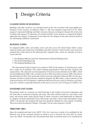
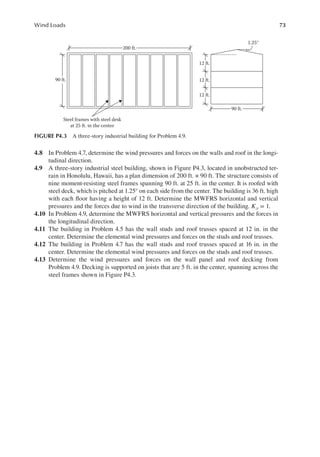
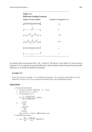
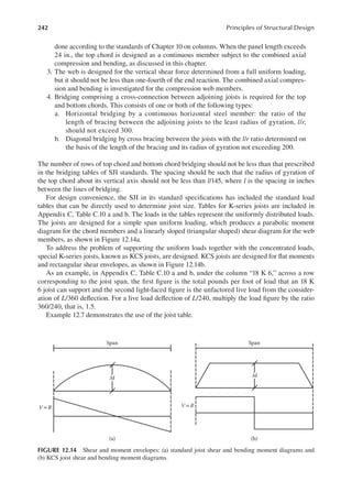
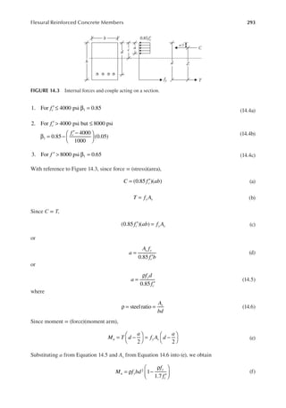
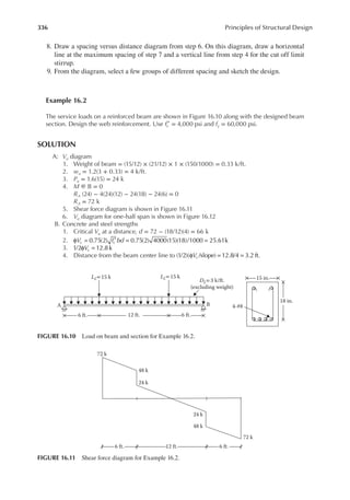
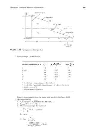
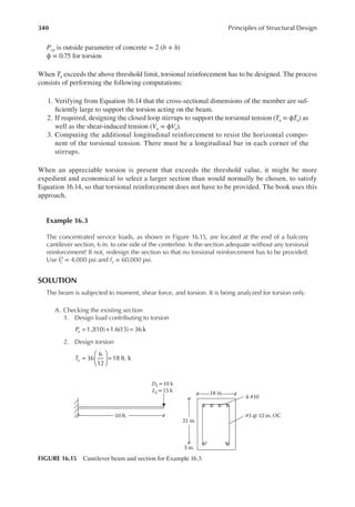
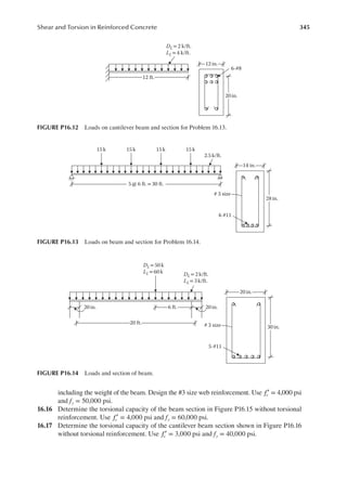
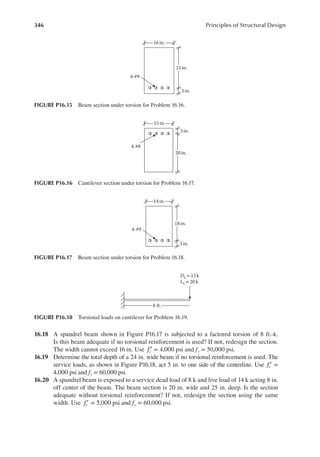
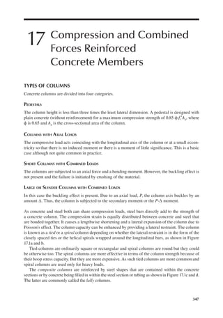
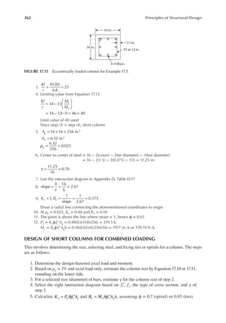
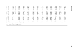
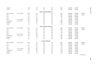
37. 19
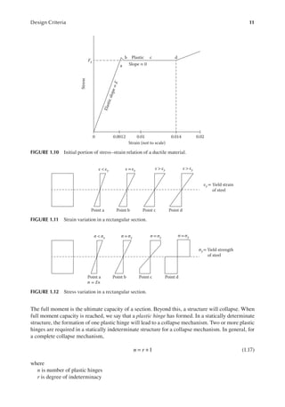
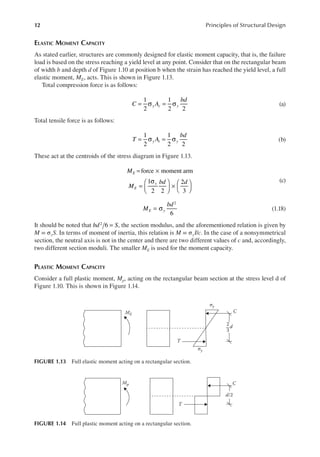
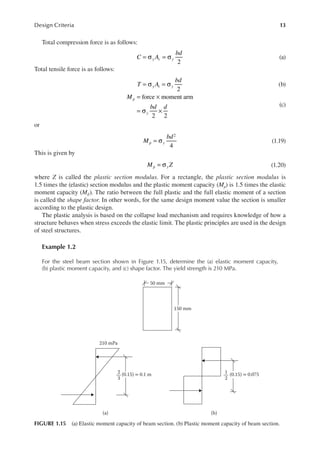
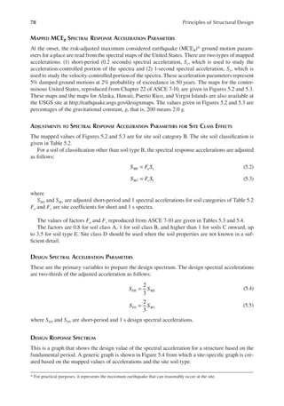
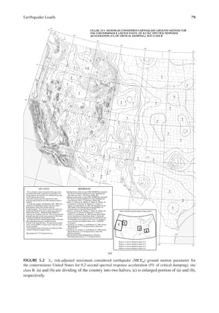
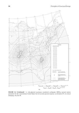
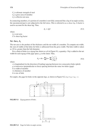
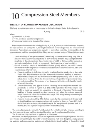
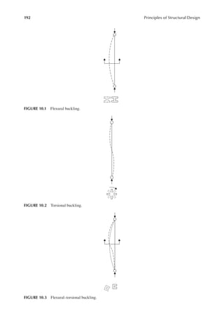
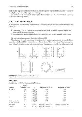
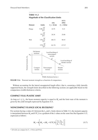
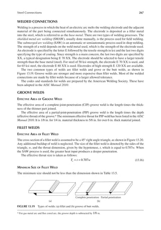
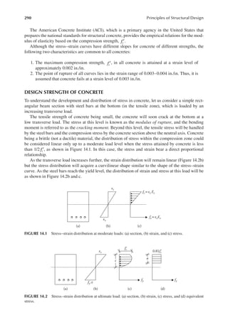
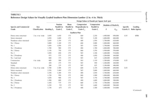
Design Criteria
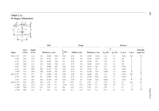
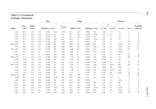
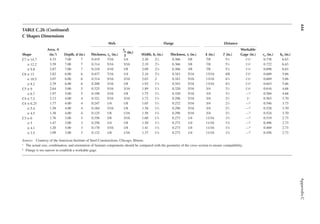
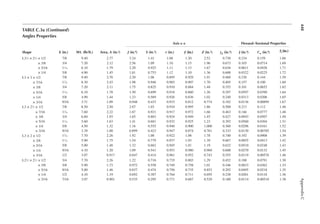
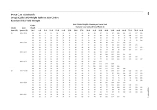
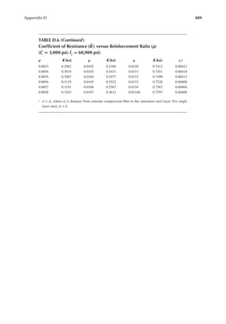
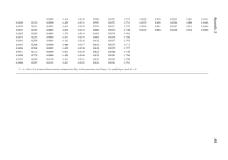
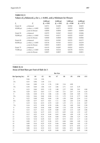
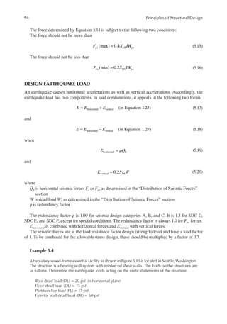
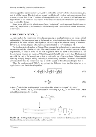
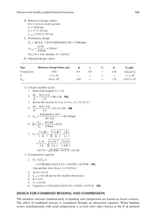
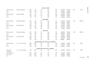
1.3 In Figure 1.6, length L = 50ft. and width B = 30 ft. and the loading is 100 lb/ft.2 Determine
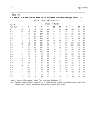
the design loads on beams GH, EF, and AD.
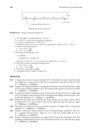
1.4 An open well is framed so that beams CE and DE sit on beam AB, as shown in Figure P1.2.
Determine the design load for beam CE and girder AB. The combined unit of dead and live
loads is 80 lb/ft.2
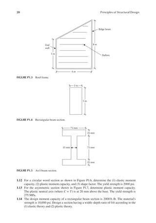
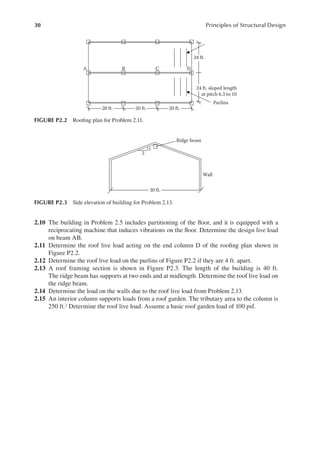
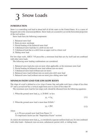
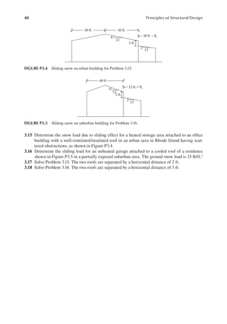
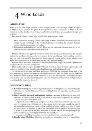
1.5 A roof is framed as shown in Figure P1.3. The load on the roof is 3 kN/m2. Determine the
design load distribution on the ridge beam.
1.6 Determine the size of the square wood column C1 from Problem 1.1 shown in Figure P1.1.
Use a resistance factor of 0.8, and assume no slenderness effect. The yield strength of wood
in compression is 4000 psi.
1.7 The service dead and live loads acting on a round tensile member of steel are 10 and 20 k,
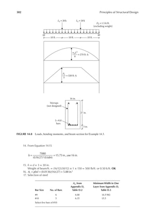
respectively. The resistance factor is 0.9. Determine the diameter of the member. The yield
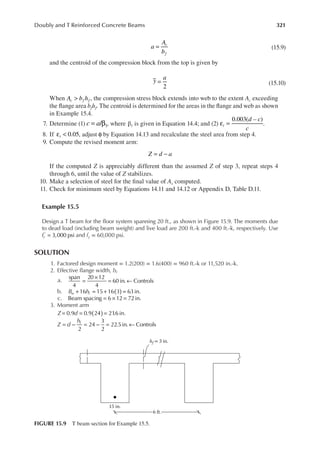
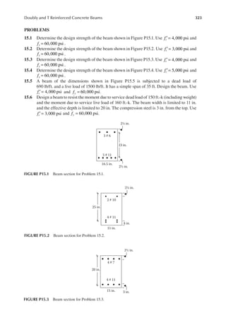
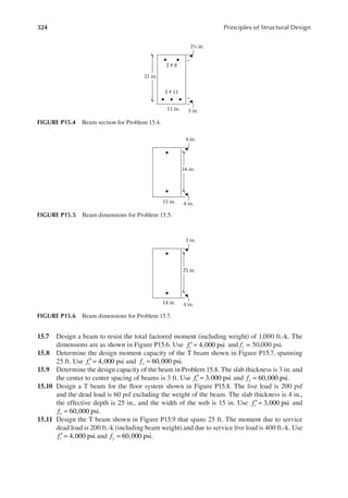
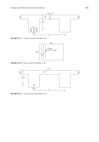
strength of steel is 36 ksi.
1.8 A steel beam spanning 30 ft. is subjected to a service dead load of 400 lb/ft. and a service
live load of 1000 lb/ft. What is the size of a rectangular beam if the depth is twice the
width? The resistance factor is 0.9. The yield strength of steel is 50 ksi.
1.9 Design the interior beam from Problem 1.1 in Figure P1.1. The resistance factor is 0.9. The
depth is three times the width. The yield strength of wood is 4000 psi.
1.10 For a steel beam section shown in Figure P1.4, determine the (1) elastic moment capacity,
(2) plastic moment capacity, and (3) shape factor. The yield strength is 50 ksi.
1.11 For the steel beam section shown in Figure P1.5, determine the (1) elastic moment capacity,
(2) plastic moment capacity, and (3) shape factor. The yield strength is 210 MPa.
[Hint: For elastic moment capacity, use the relation ME = σyI/c. For plastic capacity, ind
the compression (or tensile) forces separately for web and lange of the section and apply
these at the centroid of the web and lange, respectively.]
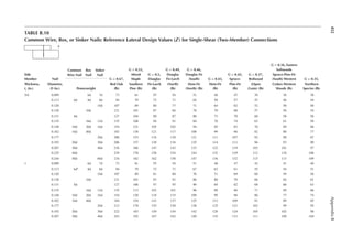
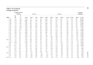
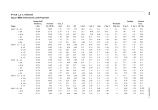
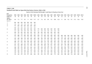
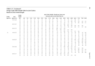
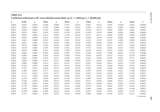
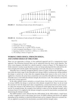
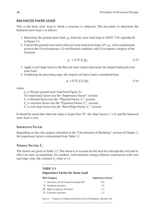
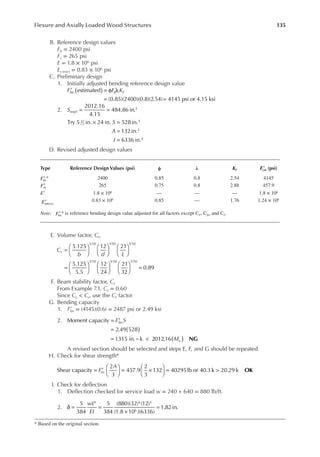
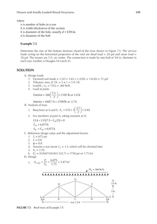
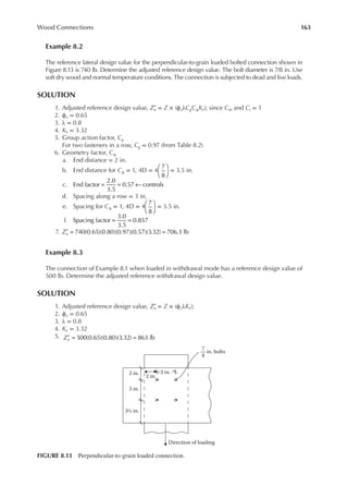
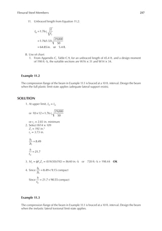
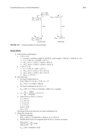
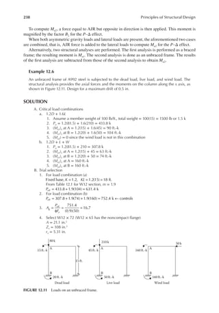
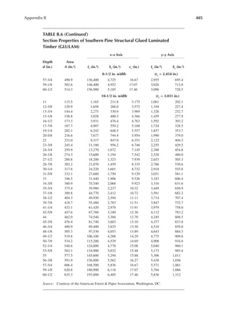
12 ft.
20 ft. 20 ft.
C1
14 ft.
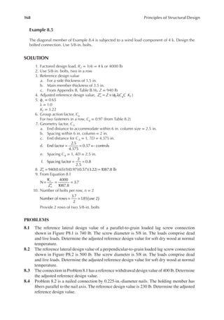
2 in. × 6 in. joists at 24 in. on center (OC)
FIGURE P1.1 Floor framing plan.
C D
Open
30 ft.
15 ft. 15 ft.
E
A B
Joists
FIGURE P1.2 An open well framing plan.

38. 20 Principles of Structural Design
1.12 For a circular wood section as shown in Figure P1.6, determine the (1) elastic moment
capacity, (2) plastic moment capacity, and (3) shape factor. The yield strength is 2000 psi.
1.13 For the asymmetric section shown in Figure P1.7, determine plastic moment capacity.
The plastic neutral axis (where C = T) is at 20 mm above the base. The yield strength is
275 MPa.
1.14 The design moment capacity of a rectangular beam section is 2000ft.·lb. The material’s
strength is 10,000 psi. Design a section having a width–depth ratio of 0.6 according to the
(1) elastic theory and (2) plastic theory.
2 in.
5 in.
FIGURE P1.4 Rectangular beam section.
75 mm
25 mm
25 mm
75 mm
25 mm
FIGURE P1.5 An I-beam section.
End
wall
5 m
6 m
8 m
Ridge beam
Rafters
FIGURE P1.3 Roof frame.

39. 21
Design Criteria
1.15 For Problem 1.14, design a circular section.
1.16 The following vertical loads are applied on a structural member. Determine the critical
vertical load in pounds per square foot for all the ASCE 7-10 combinations.
1. Dead load (on a 15° inclined member): 10 psf
2. Roof live load: 20 psf
3. Wind load (vertical component): 15 psf
4. Snow load: 30 psf
5. Earthquake load (vertical only): 2 psf
1.17 A loor beam supports the following loads. Determine the load diagrams for the various
load combinations.
1. Dead load: 1.15 k/ft.
2. Live load: 1.85 k/ft.
3. Wind load (horizontal): 15 k
4. Earthquake load (horizontal): 20 k
5. Earthquake load (vertical): 0.3 k/ft.
1.18 A simply supported loor beam is subject to the loads shown in Figure P1.8. Determine the
loading diagrams for various load combinations.
1.19 A beam supports the loads, shown in Figure P1.9. Determine the load diagrams for various
load combinations.
1.20 In Problem 1.18, if load case 5 controls the design, determine the maximum axial force,
shear force, and bending moment for which the beam should be designed.
1.21 How does the structural integrity of a building is ensured?
1.22 A three-story building has a total weight of 1000 k. The heights of the irst, second, and
third loors are 10, 9, and 8 ft., respectively. Determine the magnitudes of the minimum
notional lateral forces that have to be considered for the structural integrity of the building
assuming that the weight of the building is distributed according to the height of the loors.
10 in.
FIGURE P1.6 A circular wood section.
200 mm
100 mm
20 mm
20 mm
FIGURE P1.7 An asymmetric section.

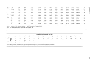
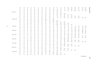
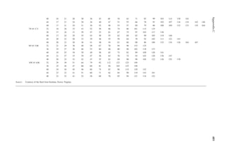
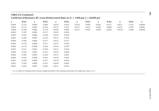
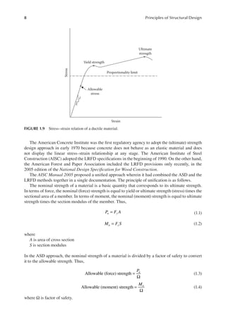
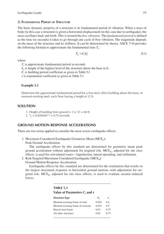
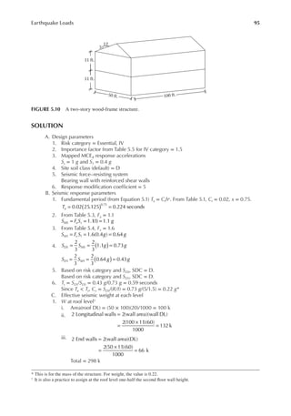
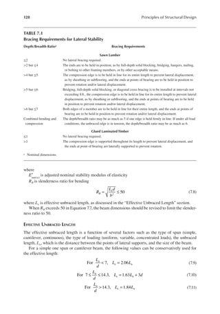
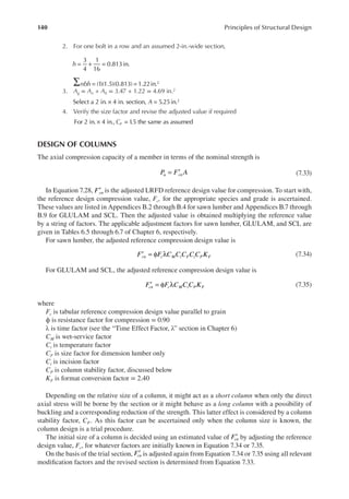
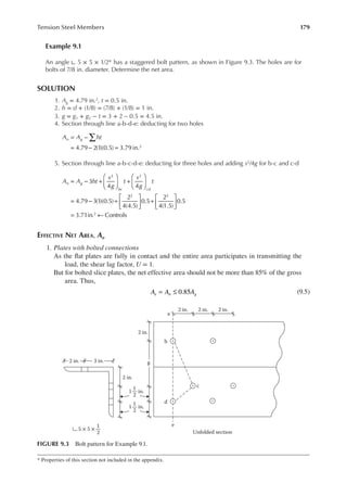
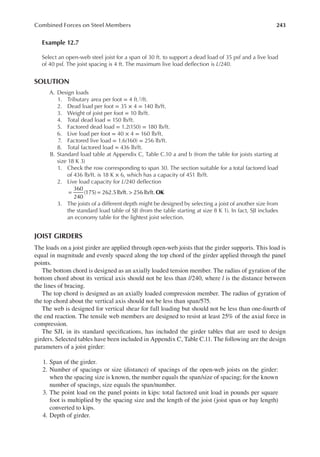
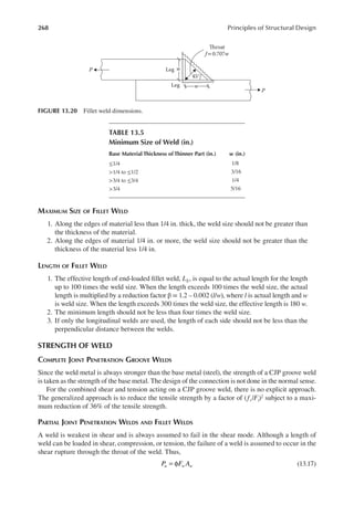
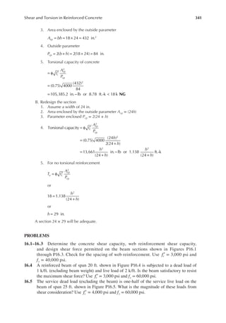
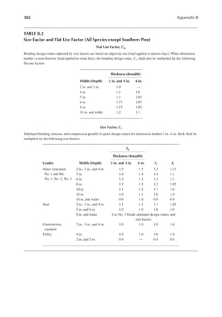
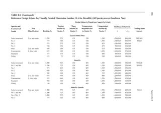
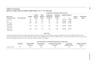
40. 22 Principles of Structural Design
1.23 Two end walls in shorter dimension (width) support the loor slabs of the building in
Problem 1.22. Determine the notional forces on the anchorages at each loor level. The
wall load is 40 psf.
[Hint: The weight of the wall assigned to each loor is according to the effective height of
the wall for each loor.]
1.24 A girder of 40 ft. span is supported at two ends. It has a dead load of 1 k/ft. and a live load
of 2 k/ft. A positive connection is provided at each end between the girder and the sup-
ports. Determine the notional force for which the connection should be designed.
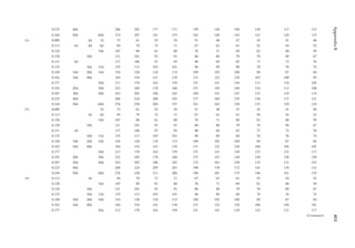
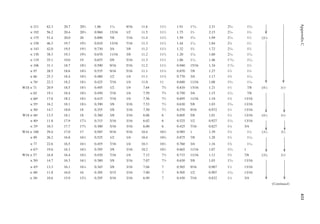
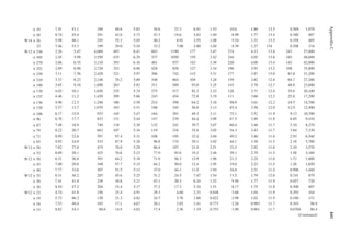
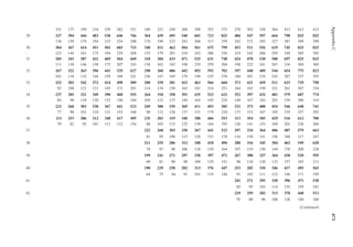
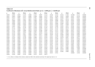
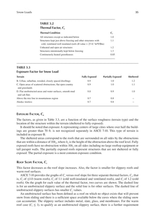
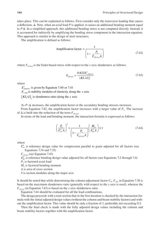
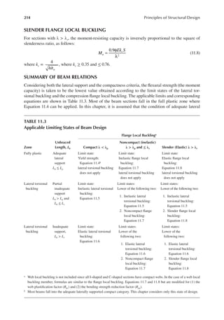
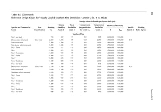
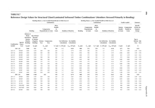
DL 12 kN
SL 30 kN
5 m
10 m
DL 1.8 k/ft.
Seismic 37.5 kN
Wind 27 kN
LL 3.15 k/ft.
FIGURE P1.9 Loads on a beam for Problem 1.19.
DL 8 kN
Transferred from roof
SL 20 kN
Lr 15 L
10 ft.
30 ft.
Seismic load 25 k
Wind load 18 k
DL 1.2k/ft.
LL 2.1k/ft.
FIGURE P1.8 Loads on a beam for Problem 1.18.

41. 23
2 Primary Loads
Dead Loads and Live Loads
DEAD LOADS
Dead loads are due to the weight of all materials that constitute a structural member. This also
includes the weight of ixed equipment that are built into the structure, such as piping, ducts, air
conditioning, and heating equipment. The speciic or unit weights of materials are available from
different sources. Dead loads are, however, expressed in terms of uniform loads on a unit area (e.g.,
pounds per square foot). The weights are converted to dead loads taking into account the tributary
area of a member. For example, a beam section weighting 4.5 lb/ft. when spaced 16 in. (1.33 ft.) on
center will have a uniform dead load of 4.5/1.33 = 3.38 psf. If the same beam section is spaced 18 in.
(1.5 ft.) on center, the uniform dead load will be 4.5/1.5 = 3.5 psf. The spacing of a beam section
may not be known to begin with, as this might be an objective of the design.
Moreover, the estimation of dead load of a member requires knowledge as to what items and
materials constitute that member. For example, a wood roof comprises roof covering, sheathing,
framing, insulation, and ceiling.
It is expeditious to assume a reasonable dead load for a structural member, only to be revised
when found grossly out of order.
The dead load of a building of light frame construction is about 10 lb/ft.2 for a looring or rooing
system without plastered ceilings and 20 lb/ft.2 with plastered ceilings. For a concrete looring sys-
tem, each 1 in. thick slab has a uniform load of about 12 psf; this is 36 psf for a 3 in. slab. To this, at
least 10 psf should be added for the supporting system. Dead loads are gravity forces that act verti-
cally downward. On a sloped roof, the dead load acts over the entire inclined length of the member.
Example 2.1
The framing of a roof consists of the following: asphalt shingles (2 psf), 0.75 in. plywood (2.5 psf),
2 × 8 framing at 12 in. on center (2.5 psf), iberglass 0.5 in. insulation (1 psf), and plastered ceiling
(10 psf). Determine the roof dead load. Make provisions for rerooing (3 psf).
SOLUTION
Dead Load (psf)
Shingles 2
Plywood 2.5
Framing 2.5
Insulation 1
Ceiling 10
Rerooing 3
Roof dead load 21

42. 24 Principles of Structural Design
LIVE LOADS
Live loads also act vertically down like dead loads but are distinct from the latter as they are not
an integral part of the structural element. Roof live loads, Lr, are associated with maintenance of a
roof by workers, equipment, and material. They are treated separately from the other types of live
loads, L, that are imposed by the use and occupancy of the structure. ASCE 7-10 speciies the mini-
mum uniformly distributed load or the concentrated load that should be used as a live load for an
intended purpose. Both the roof live load and the loor live load are subjected to a reduction when
they act on a large tributary area since it is less likely that the entire large area will be loaded to the
same magnitude of high unit load. This reduction is not allowed when an added measure of safety
is desired for important structures.
FLOOR LIVE LOADS
The loor live load is estimated by the equation
0
L kL
= (2.1)
where
L0 is basic design live load (see the section “Basic Design Live Load, L0”).
k is area reduction factor (see the section “Effective Area Reduction Factor”).
BASIC DESIGN LIVE LOAD, L0
ASCE 7-10 provides a comprehensive table for basic design loads arranged by occupancy and use of
a structure. This has been consolidated under important categories in Table 2.1.
To generalize, the basic design live loads are as follows:
Above-the-ceiling storage areas: 20 psf; one- or two-family sleeping areas: 30 psf; normal use
rooms: 40 psf; special use rooms (ofice, operating, reading, and ixed sheet arena): 50–60 psf; pub-
lic assembly places: 100 psf; lobbies, corridors, platforms, and stadium*: 100 psf for irst loor and
80 psf for other loors; light industrial uses: 125 psf; and heavy industrial uses: 250 psf.
EFFECTIVE AREA REDUCTION FACTOR
Members that have more than 400 ft.2 of inluence area are subject to a reduction in basic design
live loads. The inluence area is deined as the tributary area, AT, multiplied by an element factor,
KLL, as listed in Table 2.2.
The following cases are excluded from the live load reduction:
1. Heavy live loads that exceed 100 psf
2. Passenger car garages
3. Public assembly areas
Except the aforementioned three items, for all other cases the reduction factor is given by
0.25
15
k
K A
LL T
= +





 (2.2)
* In addition to vertical loads, horizontal swaying forces are applied to each row of sheets as follows: 24 lb per linear foot
of seat in the direction parallel to each row of sheets and 10 lb per linear foot of sheet in the direction perpendicular to
each row of sheets. Both the horizontal forces need not be applied simultaneously.

43. 25
Primary Loads
TABLE 2.1
Summarized Basic Design Live Loads
Category Uniform Load (psf)
Residential
Storage area 20
Sleeping area (dwelling) 30
Living area, stairs (dwelling) 40
Hotel room 40
Garage 40
Ofice 50
Computer room/facility 100
School classroom 40
Hospital
Patient room 40
Operation room/lab 60
Library
Reading room 60
Stacking room 150
Industrial manufacturing/warehouse
Light 125
Heavy 250
Corridor/lobby
First loor 100
Above irst loor 80
Public placesa 100
a Balcony, ballroom, ire escape, gymnasium, public stairs/exits,
restaurant, stadium, store, terrace, theater, yard, and so on.
TABLE 2.2
Live Load Element Factor, KLL
Structure Element KLL
Interior columns 4
Exterior columns without cantilever slabs 4
Edge columns with cantilever slabs 3
Corner columns with cantilever slabs 2
Edge beams without cantilever slabs 2
Interior beams 2
All other members not identiied including the
following:
1
Edge beams with cantilever slabs
Cantilever beams
One-way slabs
Two-way slabs
Note: Members without provisions for continuous shear transfer
normal to their span.

44. 26 Principles of Structural Design
As long as the following limits are observed, Equation 2.2 can be applied to any area. However,
with the limits imposed the factor k becomes effective when KLLAT is greater than 400, as stated
earlier:
1. The k factor should not be more than 1.
2. The k factor should not be less than 0.5 for members supporting one loor and 0.4 for
members supporting more than one loor.
Example 2.2
The irst loor framing plan of a single family dwelling is shown in Figure 2.1. Determine the mag-
nitude of live load on the interior column C.
SOLUTION
1. From Table 2.1, L0 = 40 psf
2. Tributary area AT = 20 × 17.5 = 350 ft.2
3. From Table 2.2, KLL = 4
4. KLLAT = 4 × 350 = 1400
5. From Equation 2.2
0.25
15
0.25
15
1400
0.65
= +






= +





 =
K
K A
LL T
6. From Equation 2.1, L = kL0 = 0.65 (40) = 26 psf
OTHER PROVISIONS FOR FLOOR LIVE LOADS
Besides uniformly distributed live loads, ASCE 7-10 also indicates the concentrated live loads in
certain cases that are assumed to be distributed over an area of 2.5 ft. × 2.5 ft. The maximum effect
of either the uniformly distributed load or the concentrated load has to be considered. In most cases,
the uniformly distributed loads have higher magnitudes.
In buildings where partitions are likely to be erected, a uniform partition live load is provided in
addition to the basic design loads. The minimum partition load is 15 psf. Partition live loads are not
subjected to reduction for large effective areas.
A B
60 ft.
Beam
35 ft.
Joists
C D
FIGURE 2.1 Floor framing plan.

45. 27
Primary Loads
Live loads include an allowance for an ordinary impact. However, where unusual vibrations and
impact forces are involved live loads should be increased. The moving loads shall be increased
by an impact factor as follows: (1) elevator, 100%; (2) light shaft or motor-driven machine, 20%;
(3) reciprocating machinery, 50%; and (4) hangers for loor or balcony, 33%. After including these
effects,
Total LL/unit area = unit LL (1 IF) PL {min 15 psf}
+ + (2.3)
where
LL is live load
IF is impact factor, in decimal point
PL is partition load
MULTIPLE FLOORS REDUCTIONS
In one- and two-family dwellings, for members supporting more than one loor load the following
live load reduction is permitted as an alternative to Equations 2.1 and 2.2:
L L L L
0.7 ( )
01 02 03
= + + + … (2.4)
where L01, L02, … are the unreduced loor live loads applied on each of the multiple story levels
regardless of tributary area. The reduced loor live load, L, should not be less than the largest unre-
duced loor live load on any one story level acting alone.
Example 2.3
An interior column supports the following unit live loads from three loors on a surface area of
20 ft. × 30 ft. each: irst loor = 35 psf, second loor = 30 psf, and third loor = 25 psf. Determine
the design unit live load on the column.
SOLUTION
1. Total load = 35 + 30 + 25 = 90 psf
2. Tributary area AT = 20 × 30 = 600 ft.2
3. From Table 2.2, KLL = 4
4. KLLAT = 4 × 600 = 2400 ft.2
5. From Equation 2.2
= +





 =
k 0.25
15
2400
0.556
6. From Equation 2.1
L = kL0 = 0.556 (90) = 50 psf
7. From the alternative equation (Equation 2.4)
L = 0.7 × (35 + 30 + 25) = 63 psf ← controls
Live load should not be less than maximum on any loor of 35 psf.

46. 28 Principles of Structural Design
ROOF LIVE LOADS, Lr
Roof live loads happen for a short time during the rooing or rerooing process. In load combina-
tions, either the roof live load, Lr, or the snow load, S, is included, since both of these are not likely
to occur simultaneously.
The standard roof live load for ordinary lat, sloped, or curved roofs is 20 psf. This can be
reduced to a minimum value of 12 psf based on the tributary area being larger than 200 ft.2 and/or
the roof slope being more than 18.4°. When less than 20 psf of roof live loads are applied to a con-
tinuous beam structure, the reduced roof live load is applied to adjacent spans or alternate spans,
whichever produces the greatest unfavorable effect.
The roof live load is estimated by
1 2 0
L R R L
r = (2.5)
where
Lr is reduced roof live load on a horizontally projected surface
L0 is basic design load for ordinary roof, which is 20 psf
R1 is tributary area reduction factor (see the section “Tributary Area Reduction Factor, R1”)
R2 is slope reduction factor (see the section “Slope Reduction Factor”)
TRIBUTARY AREA REDUCTION FACTOR, R1
This is given by
1.2 0.001
1
R AT
= − (2.6)
where AT is the horizontal projection of roof tributary area in square feet.
This is subject to the following limitations:
1. R1 should not exceed 1.
2. R1 should not be less than 0.6.
SLOPE REDUCTION FACTOR
This is given by
1.2 0.6 tan
2 = − θ
R (2.7)
where θ is the roof slope angle.
This is subject to the following limitations:
1. R2 should not exceed 1.
2. R2 should not be less than 0.6.
Example 2.4
The horizontal projection of a roof framing plan of a building is similar to Figure 2.1. The roof pitch
is 7 on 12. Determine the roof live load acting on column C.

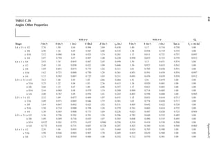
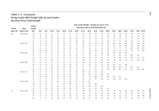
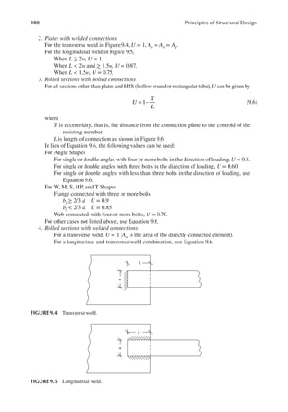
47. 29
Primary Loads
SOLUTION
1. L0 = 20 psf
2. AT = 20 × 17.5 = 350 ft.2
3. From Equation 2.6, R1 = 1.2 – 0.001 (350) = 0.85
4. Pitch of 7 on 12, tan θ = 7/12 or θ = 30.256°
5. From Equation 2.7, R2 = 1.2 − 0.6 tan 30.256° = 0.85
6. From Equation 2.5, Lr = (0.85) (0.85) (20) = 14.45 psf > 12 psf OK
The aforementioned computations are for an ordinary roof. Special purpose roofs such as roof
gardens have loads up to 100 psf. These are permitted to be reduced according to loor live load
reduction, as discussed in the “Floor Live Loads” section.
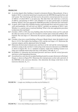
PROBLEMS
2.1 A loor framing consists of the following: hardwood loor (4 psf), 1 in. plywood (3 psf),
2 in. × 12 in. framing at 4 in. on center (2.6 psf), ceiling supports (0.5 psf), and gypsum
wallboard ceiling (5 psf). Determine the loor dead load.
2.2 In Problem 2.1, the loor covering is replaced by a 1 in. concrete slab and the framing by
2 in. × 12 in. at 3 in. on center. Determine the loor dead load.
[Hint: Weight in pounds of concrete/unit area = 1 ft. × 1 ft. × 1/12 ft. × 150.]
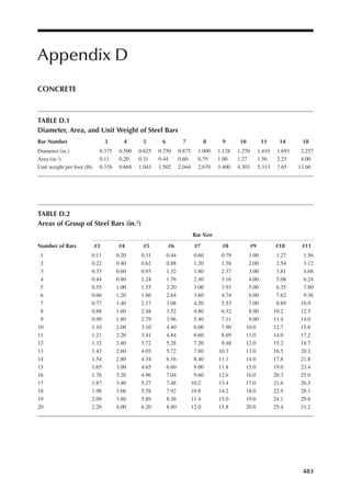
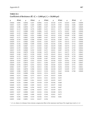
2.3 For the loor framing plan of Example 2.2, determine the design live load on the interior
beam BC.
2.4 An interior steel column of an ofice building supports a unit load, as indicated in Table 2.1,
from the loor above. The column to column distance among all columns in the loor plan
is 40 ft. Determine the design live load on the column.
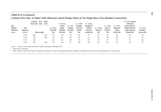
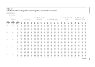
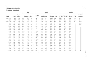
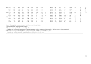
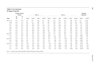
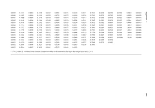
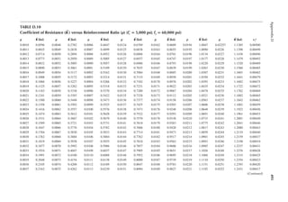
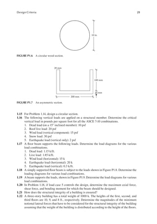
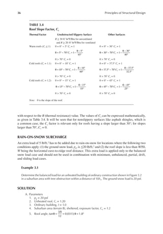
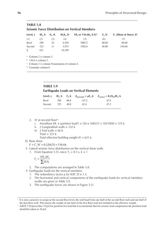
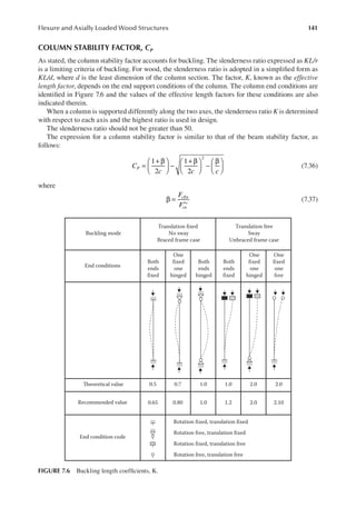
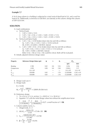
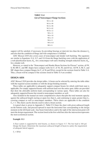
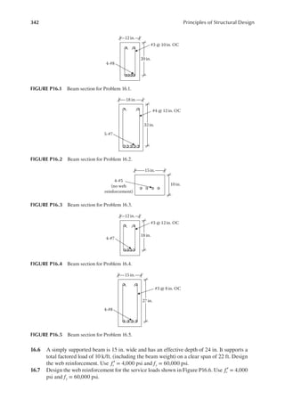
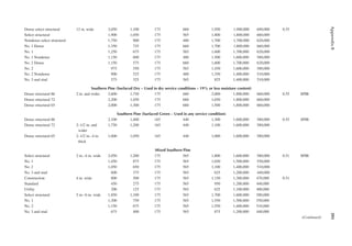
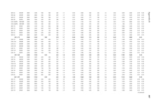
2.5 The framing plan of a gymnasium is shown in Figure P2.1. Determine the live load on
column A.
2.6 Determine the live load on the slab resting on column A from Problem 2.5.
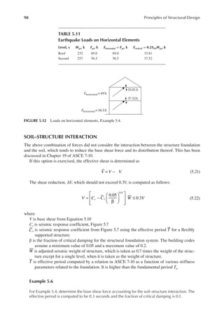
2.7 The column in Problem 2.4 supports the same live loads from two loors above. Determine
the design live load on the column.
2.8 A corner column with a cantilever slab supports the following live loads over an area of
25 ft. × 30 ft. Determine the design live load. First loor = 30 psf, second loor = 25 psf,
and third loor = 20 psf.
2.9 The column in Problem 2.8 additionally supports an elevator and hangers of a balcony.
Determine the design load.
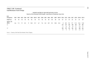
A B
20 ft.
50 ft.
50 ft.
20 ft.
20 ft.
FIGURE P2.1 Framing plan for Problem 2.5.

48. 30 Principles of Structural Design
2.10 The building in Problem 2.5 includes partitioning of the loor, and it is equipped with a
reciprocating machine that induces vibrations on the loor. Determine the design live load
on beam AB.
2.11 Determine the roof live load acting on the end column D of the rooing plan shown in
Figure P2.2.
2.12 Determine the roof live load on the purlins of Figure P2.2 if they are 4 ft. apart.
2.13 A roof framing section is shown in Figure P2.3. The length of the building is 40 ft.
The ridge beam has supports at two ends and at midlength. Determine the roof live load on
the ridge beam.
2.14 Determine the load on the walls due to the roof live load from Problem 2.13.
2.15 An interior column supports loads from a roof garden. The tributary area to the column is
250 ft.2 Determine the roof live load. Assume a basic roof garden load of 100 psf.
A B
20 ft. 20 ft.
20 ft.
24 ft. sloped length
at pitch 6.3 to 10
24 ft.
Purlins
C D
FIGURE P2.2 Rooing plan for Problem 2.11.
30 ft.
Wall
Ridge beam
1
2
FIGURE P2.3 Side elevation of building for Problem 2.13.

49. 31
3 Snow Loads
INTRODUCTION
Snow is a controlling roof load in about half of all the states in the United States. It is a cause of
frequent and costly structural problems. Snow loads are assumed to act on the horizontal projection
of the roof surface.
Snow loads have the following components:
1. Balanced snow load
2. Rain-on-snow surcharge
3. Partial loading of the balanced snow load
4. Unbalanced snow load due to a drift on one roof
5. Unbalanced load due to a drift from an upper roof to a lower roof
6. Sliding snow load
For low-slope roofs, ASCE 7-10 prescribes a minimum load that acts by itself and not combined
with other snow loads.
The following snow loading combinations are considered:
1. Balanced snow load plus rain-on-snow when applicable, or the minimum snow load
2. Partial loading (of balanced snow load without rain-on-snow)
3. Unbalanced snow load (without rain-on-snow)
4. Balanced snow load (without rain-on-snow) plus drift snow load
5. Balanced snow load (without rain-on-snow) plus sliding snow load
MINIMUM SNOW LOAD FOR LOW-SLOPE ROOFS
The slope of a roof is deined as a low slope if mono, hip, and gable roofs have a slope of less than
15° and a curved roof has a vertical angle from eave to crown of less than 10°.
The minimum snow load for low-slope roofs should be obtained from the following equations:
1. When the ground snow load, pg, is 20 lb/ft.2 or less
=
p I p
m g (3.1)
2. When the ground snow load is more than 20 lb/ft.2
20
=
p I
m (3.2)
where
pg is 50-year ground snow load from Figure 3.1
I is importance factor (see the “Importance Factor” section)
As stated, the minimum snow load, pm, is considered a separate uniform load case. It is not combined
with other loads—balanced, rain-on-snow, unbalanced, partial, drift, or sliding loads.

50. 32 Principles of Structural Design
(200)
10
(100)
5
(200)
20
(700)
20
(1000)
20
(800)
15
(600)
10
(2800)
20
(1500)
15
(1500)
20
(1200)
10
(3300)
20
(4000)
20
(3400)
15
(4600)
20
(6000)
15
(5000)
10
(3200)
20
(4600)
20
(5400)
20
CS
CS
CS
(4600)
15
(3800)
10
(6600)
15
(6000)
35
(6000)
30
(6000)
25
(4600)
10
(5200)
20
(4500)
15
(5000)
15
(6000)
15
(4500)
10
(3600)
5
(2000)
ZERO
(3600)
5 (5400)
10
(4500)
5
(3000)
ZERO
(5000)
10
(4000)
5
(3500)
ZERO
(6300)
15
(5400)
10
(4500)
5
(3000)
ZERO
(6800)
15
(6400)
10
(6000)
5
(2000)
ZERO
(2000)
ZERO
(3000)
ZERO
(6000)
15
(6200)
20
(6500)
15
(5000)
10
(4800)
5
(4400)
10
(3200)
5
(3600)
10
(5000)
5
(3500)
ZERO
(6000)
10
(5000)
5
(4500)
ZERO
ZERO
5
10
20
20
15
20
15
(5000)
10
25
30
35
40
50
40
35
CS
35
25
(3700)
30
50
(2600)
30
60
20
(1000)
ZERO
(2800)
5
(1800)
ZERO
(2000)
5
(1500)
ZERO
(1500)
ZERO
(5000)
10
(4400)
10
(4300)
20
(4100)
15
(3200)
10
(800)
5
CS
CS
CS
CS
CS
CS
CS
(4000)
5
(2400)
ZERO
(6400)
15
CS CS
(3000)
25
(3600)
20
(4100)
25
(4800)
25
(4500)
20
(5500)
15
(6500)
15
CS
CS
CS
(400)
15
(400)
10
(300)
5
(500)
5
(300)
ZERO
(1800)
10
(1300)
5
(600)
ZERO
(4000)
ZERO
(3000)
ZERO
In CS areas, site-specific case studies are required to
establish ground snow loads. Extreme local variations
in ground snow loads in these areas preclude mapping
at this scale.
Numbers in parentheses represent the upper elevation limits
in feet for the ground snow load values presented below.
Site-specific case studies are required to establish ground
snow loads at elevations not covered.
To convert Ib/sq ft. to kN/m
2
, multiply by 0.0479.
To convert feet to meters, multiply by 0.3048.
0
(a)
100 200 300 miles
(4500)
20
FIGURE 3.1 Ground snow loads, pg, for the United States. The entire country is divided in two parts. (a) and
(b) distinguishes two parts. (Courtesy of American Society of Civil Engineers, Reston, VA.)

51. 33
Snow Loads
70
100
CS
CS
CS
CS
CS
CS CS CS
CS
50
50
50
50 40
40 30
30
35
35 25
25
25
25
25
15
5
5
5
ZERO
ZERO
10
10
30
30
30
40
(1700)
30
(1700)
30
(800)
35
(1000)
35
300
20
20
20
20
(1800)
10
(2500)
15
(2500)
20
(1200)
25
(2500)
25
20
60
60
60
70
70
(1000)
40
(1000)
60
40
(800)
60
(700)
50
(700)
90
(700)
100
(900)
50
(600)
80
(500)
60
(500)
70
(500)
50 (900)
50
35
35
25
25
25
(b)
90
15
FIGURE 3.1 (continued) Ground snow loads, pg, for the United States. (Courtesy of American Society of
Civil Engineers, Reston, VA.)

52. 34 Principles of Structural Design
BALANCED SNOW LOAD
This is the basic snow load to which a structure is subjected. The procedure to determine the
balanced snow load is as follows:
1. Determine the ground snow load, pg, from the snow load map in ASCE 7-10, reproduced
in Figure 3.1.
2. Convert the ground snow load to lat roof snow load (roof slope ≤5°), pf, with consideration
given to the (1) roof exposure, (2) roof thermal condition, and (3) occupancy category of the
structure:
0.7
=
p C C Ip
f e t g (3.3)
3. Apply a roof slope factor to the lat roof snow load to determine the sloped (balanced) roof
snow load.
4. Combining the preceding steps, the sloped roof snow load is calculated from
0.7
=
p C C C Ip
s s e t g (3.4)
where
pg is 50-year ground snow load from Figure 3.1
I is importance factor (see the “Importance Factor” section)
Ct is thermal factor (see the “Thermal Factor, Ct” section)
Ce is exposure factor (see the “Exposure Factor, Ce” section)
Cs is roof slope factor (see the “Roof Slope Factor, Cs” section)
It should be noted that when the slope is larger than 70°, the slope factor Cs = 0, and the balanced
snow load is zero.
IMPORTANCE FACTOR
Depending on the risk category identiied in the “Classiication of Buildings” section of Chapter 1,
the importance factor is determined from Table 3.1
THERMAL FACTOR, Ct
The factors are given in Table 3.2. The intent is to account for the heat loss through the roof and its
effect on snow accumulation. For modern, well-insulated, energy-eficient construction with eave
and ridge vents, the common Ct value is 1.1.
TABLE 3.1
Importance Factor for Snow Load
Risk Category Importance Factor
I. Structures of low hazard to human life 0.8
II. Standard structures 1.0
III. High occupancy structures 1.1
IV. Essential structures 1.2
Source: Courtesy of American Society of Civil Engineers, Reston, VA.

53. 35
Snow Loads
EXPOSURE FACTOR, Ce
The factors, as given in Table 3.3, are a function of the surface roughness (terrain type) and the
location of the structure within the terrain (sheltered to fully exposed).
It should be noted that exposure A representing centers of large cities where over half the build-
ings are greater than 70 ft. is not recognized separately in ASCE 7-10. This type of terrain is
included in exposure B.
The sheltered areas correspond to the roofs that are surrounded on all sides by the obstructions
that are within a distance of 10ho, where ho is the height of the obstruction above the roof level. Fully
exposed roofs have no obstruction within 10ho on all sides including no large rooftop equipment or
tall parapet walls. The partially exposed roofs represent structures that are not sheltered or fully
exposed. The partial exposure is a most common exposure condition.
ROOF SLOPE FACTOR, CS
This factor decreases as the roof slope increases. Also, the factor is smaller for slippery roofs and
warm roof surfaces.
ASCE 7-10 provides the graphs of Cs versus roof slope for three separate thermal factors, Ct, that
is, Ct of ≤1.0 (warm roofs), Ct of 1.1 (cold well-insulated and ventilated roofs), and Ct of 1.2 (cold
roofs). On the graph for each value of the thermal factor, two curves are shown. The dashed line
is for an unobstructed slippery surface and the solid line is for other surfaces. The dashed line of
unobstructed slippery surfaces has smaller Cs values.
An unobstructed surface has been deined as a roof on which no object exists that will prevent
snow from sliding and there is a suficient space available below the eaves where the sliding snow
can accumulate. The slippery surface includes metal, slate, glass, and membranes. For the warm
roof case (Ct ≤ 1), to qualify as an unobstructed slippery surface, there is a further requirement
TABLE 3.2
Thermal Factor, ct
Thermal Condition ct
All structures except as indicated below 1.0
Structures kept just above freezing and other structures with
cold, ventilated well insulated roofs (R-value > 25 ft.2 hr0F/Btu)
1.1
Unheated and open air structures 1.2
Structures intentionally kept below freezing 1.3
Continuously heated greenhouses 0.85
TABLE 3.3
Exposure Factor for Snow Load
Terrain Fully Exposed Partially Exposed Sheltered
B. Urban, suburban, wooded, closely spaced dwellings 0.9 1.0 1.2
C. Open areas of scattered obstructions, lat open country
and grasslands
0.9 1.0 1.1
D. Flat unobstructed areas and water surfaces, smooth mud
and salt lats
0.8 0.9 1.0
Above the tree line in mountainous region 0.7 0.8 –
Alaska: treeless 0.7 0.8 –

54. 36 Principles of Structural Design
with respect to the R (thermal resistance) value. The values of Cs can be expressed mathematically,
as given in Table 3.4. It will be seen that for nonslippery surfaces like asphalt shingles, which is
a common case, the Cs factor is relevant only for roofs having a slope larger than 30°; for slopes
larger than 70°, Cs = 0.
RAIN-ON-SNOW SURCHARGE
An extra load of 5 lb/ft.2 has to be added due to rain-on-snow for locations where the following two
conditions apply: (1) the ground snow load, pg, is ≤20 lb/ft.2 and (2) the roof slope is less than W/50,
W being the horizontal eave-to-ridge roof distance. This extra load is applied only to the balanced
snow load case and should not be used in combination with minimum, unbalanced, partial, drift,
and sliding load cases.
Example 3.1
Determine the balanced load for an unheated building of ordinary construction shown in Figure 3.2
in a suburban area with tree obstruction within a distance of 10ho. The ground snow load is 20 psf.
SOLUTION
A. Parameters
1. pg = 20 psf
2. Unheated roof, Ct = 1.20
3. Ordinary building, I = 1.0
4. Suburban area (terrain B), sheltered, exposure factor, Ce = 1.2
5. Roof angle, θ = = θ = °
tan
3/8
12
0.0313; 1.8
TABLE 3.4
Roof Slope Factor, cs
Thermal Factor Unobstructed Slippery Surface Other Surfaces
R ≥ 30 ft2 hr0F/Btu for unventilated
and R ≥ 20 ft2 hr0F/Btu for ventilated
Warm roofs (Ct ≤ 1) θ = 0° − 5° Cs = 1 θ = 0° − 30° Cs = 1
5 70 1
5
65
Cs
θ = ° − ° = −
θ − °
°
30 70 1
30
40
Cs
θ = ° − ° = −
θ − °
°
θ > 70° Cs = 0 θ > 70° Cs = 0
Cold roofs (Ct = 1.1) θ = 0° − 10° Cs = 1 θ = 0° − 37.5° Cs = 1
10 70 1
10
60
Cs
θ = ° − ° = −
θ − °
°
37.5 70 1
37.5
32.5
Cs
θ = ° − ° = −
θ − °
°
θ > 70° Cs = 0 θ > 70° Cs = 0
Cold roofs (Ct = 1.2) θ = 0° − 15° Cs = 1 θ = 0° − 45° Cs = 1
15 70 1
15
55
Cs
θ = ° − ° = −
θ − °
°
45 70 1
45
25
Cs
θ = ° − ° = −
θ − °
°
θ > 70° Cs = 0 θ > 70° Cs = 0
Note: θ is the slope of the roof.

55. 37
Snow Loads
6. θ < 15°, it is a low slope, the minimum load equation applies
7. = =
50
125
50
2.5
W
8. θ < 2.5° and pg = 20 psf, rain-on-snow surcharge = 5 lb/ft.2
9. From Table 3.4, Cs = 1.0
B. Snow loads
1. Minimum snow load, from Equation 3.1
(1)(20) 20 lb/ft.2
= =
pm
2. From Equation 3.4
0.7
0.7(1)(1.2)(1.2)(1)(20) 20.16lb/ft.2
=
= =
p C C C Ip
s s e t g
3. Add rain-on-snow surcharge
pb 20.16 5 25.16 lb/ft. controls
2
= + = ←
Example 3.2
Determine the balanced snow load for an essential facility in Seattle, Washington, having a roof
eave to ridge width of 100 ft. and a height of 25 ft. It is a warm roof structure.
SOLUTION
A. Parameters
1. Seattle, Washington, pg = 20 psf
2. Warm roof, Ct = 1.00
3. Essential facility, I = 1.2
4. Category B, urban area, partially exposed (default), exposure factor, Ce = 1.00
5. Roof slope, θ = = θ = °
tan
25
100
0.25; 14 .
6. θ < 15°, the minimum snow equation is applicable
7. θ is not less than W/50, there is no rain-on-snow surcharge
8. For a warm roof, other structures, from Table 3.4 Cs = 1
B. Snow loads
1. = = ←
(1.2)(20) 24 lb/ft. controls
2
pm
2. p C C C Ip
s s e t g
0.7
0.7(1)(1)(1.2) 16.8 lbs/ft.2
=
= =
PARTIAL LOADING OF THE BALANCED SNOW LOAD
The partial loads are different from the unbalanced loads. In unbalanced loads, snow is removed
from one portion and is deposited in another portion. In the case of partial loading, snow is removed
from one portion through scour or melting but is not added to another portion. The intent is that in
125 ft.
125 ft.
12
3/8
FIGURE 3.2 Low-slope roof.

56. 38 Principles of Structural Design
a continuous span structure, a reduction in snow loading on one span might induce heavier stresses
in some other portion than those that occur with the entire structure being loaded. The provision
requires that a selected span or spans should be loaded with one-half of the balanced snow load
and the remaining spans with the full balanced snow load. This should be evaluated for various
alternatives to assess the greatest effect on the structural member.
Partial load is not applied to the members that span perpendicular to the ridgeline in gable roofs
having slopes 2.38° or more.
UNBALANCED ACROSS THE RIDGE SNOW LOAD
The balanced and unbalanced loads are analyzed separately.
The unbalanced loading condition results from when a blowing wind depletes snow from the
upwind direction to pile it up in the downward direction.
The unbalanced snow loading for hip and gable roofs is discussed here. For curved, saw tooth,
and dome roofs, a reference is made to Sections 7.6.2 through 7.6.4 of ASCE 7-10.
For unbalanced load to occur on any roof, it should be neither a very low-slope roof nor a steep
roof. Thus, the following two conditions should be satisied for across the ridge unbalanced snow
loading:
1. The roof slope should be equal to or larger than 2.38°.
2. The roof slope should be less than 30.2°.
When the preceding two conditions are satisied, the unbalanced load distribution is expressed
in two different ways:
1. For narrow roofs (W ≤ 20 ft.) of simple structural systems like the prismatic wood rafters or
light gauge roof rafters spanning from eave to ridge, the windward side is taken as free of
snow, and on the leeward side the total snow load is represented by a uniform load from eave
to ridge as follows (note this is the total load and is not an addition to the balanced load):
=
p Ip
u g (3.5)
2. For wide roofs (W > 20 ft.) of any structures as well as the narrow roofs of other than the
simple structures stated in the preceding discussion, the load is triangular in shape but is
represented by a more user-friendly rectangular surcharge over the balanced load.
On the windward side, a uniform load of 0.3ps is applied, where ps is the balanced snow load
mentioned in the “Balanced Snow Load” section. On the leeward side, a rectangular load is placed
adjacent to the ridge, on top of the balanced load, ps, as follows:
Uniformload, =
γ
p
h
s
u
d
(3.6)
Horizontalextentfromridge,
8
3
=
L
h s
d
(3.7)
where
1
is roof slope
s
γ is unit weight of snow in lb/ft.3, given by
0.13 14 30 lb/ft.3
γ = + ≤
pg (3.8)

57. 39
Snow Loads
hd is height of drift in feet on the leeward roof, given by
0.43( ) ( 10) 1.5
1 3 1 4
= + −
h W p
d g (3.9)
W is horizontal distance from eave to ridge for the windward portion of the roof in feet
If W < 20 ft., use W = 20 ft.
Example 3.3
Determine the unbalanced drift snow load for Example 3.1.
SOLUTION
1. Roof slope, θ = 1.8°.
2. Since roof slope <2.38°, there is no unbalanced snow load.
Example 3.4
Determine the unbalanced drift snow load for Example 3.2.
SOLUTION
A. On leeward side
1. Roof slope, θ = 14°, it is not a low-slope roof for unbalanced load.
2. W > 20 ft., it is a wide roof.
3. pg = 20 psf and ps = 16.8 lb/ft.2 (from Example 3.2).
4.
s
s
slope
1 25
100
or 4
= = =
5. h W p
d g
0.43( ) ( 10) 1.5
0.43(100) (20 10) 1.5 3.16
1 3 1 4
1 3 1 4
= + −
= + − =
6. Unit weight of snow
γ = + ≤
= + =
0.13 14 30
0.13(20) 14 16.6 lb/ft.3
pg
7. =
γ
= =
(3.16)(16.6)
4
26.23lb/ft.2
p
h
s
u
d
8. Horizontal extent, = = =
8
3
8(3.16) 4
3
16.85 ft.
L
h s
d
B. On windward side
9. pu = 0.3 ps = 0.3 (16.8) = 5.04 psf.
10. This is sketched in Figure 3.3.
16.8 psf
26.23 psf
5.04 psf
100 ft. 100 ft.
16.85 ft.
FIGURE 3.3 Unbalanced snow load on a roof.

58. 40 Principles of Structural Design
SNOW DRIFT FROM A HIGHER TO A LOWER ROOF
The snow drifts are formed in the wind shadow of a higher structure onto a lower structure. The
lower roof can be a part of the same structure or it could be an adjacent separated structure.
This drift is a surcharge that is superimposed on the balanced snow roof load of the lower roof.
The drift accumulation, when the higher roof is on the windward side, is shown in Figure 3.4. This
is known as the leeward snow drift.
When the higher roof is on the leeward side, the drift accumulation, known as the windward
snow drift, is more complex. It starts as a quadrilateral shape because of the wind vortex and ends
up in a triangular shape, as shown in Figure 3.5.
LEEWARD SNOW DRIFT ON LOWER ROOF OF ATTACHED STRUCTURE
In Figure 3.4, if hc/hb is less than 0.2, the drift load is not applied, where hb is the balanced snow
depth determined by dividing the balanced snow load, ps, by a unit load of snow, γ, computed by
Equation 3.7. The term hc represents the difference of elevation between high and low roofs sub-
tracted by hb, as shown in Figure 3.4.
The drift is represented by a triangle, as shown in Figure 3.6.
0.43( ) ( 10) 1.5
1 3 1 4
h L p
d u g
= + − (3.10)
where Lu is horizontal length of the roof upwind of the drift, as shown in Figure 3.4.
The corresponding maximum snow load is
p h
d d
= γ (3.11)
Wind
Lu
w
hd
hc
hb
FIGURE 3.4 Leeward snow drift.
LL
hc
hd
hb
Wind
FIGURE 3.5 Windward snow drift.

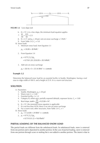
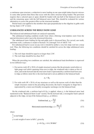
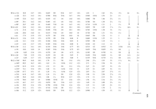
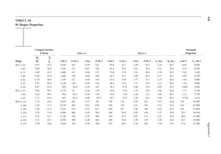
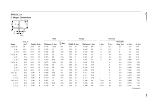
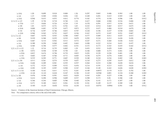
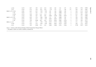
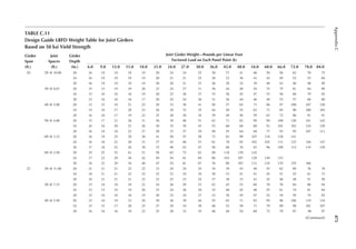
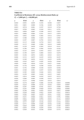
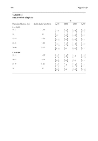
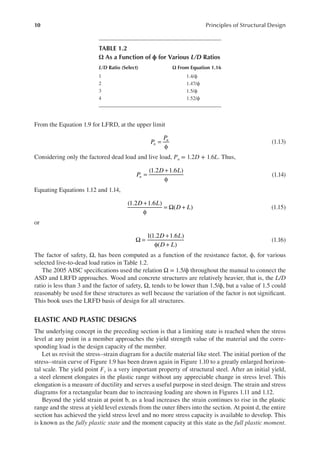
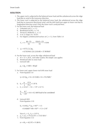
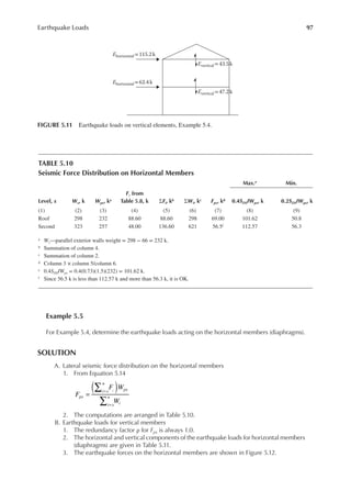
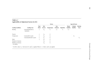
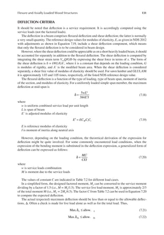
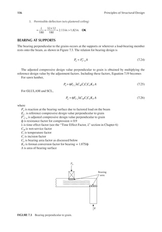
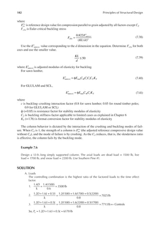
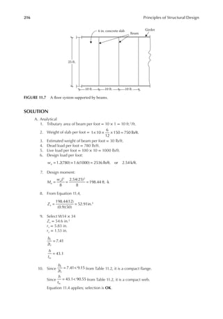
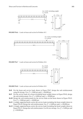
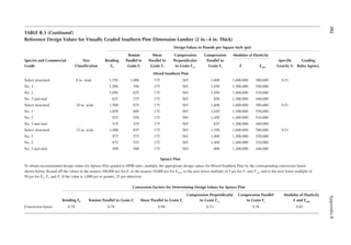
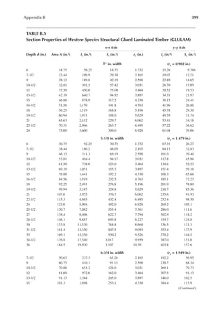
59. 41
Snow Loads
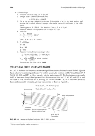
The width of the snow load (base of the triangle) has the following value for two different cases:
1. For hd ≤ hc
4
w hd
= (3.12)
2. For hd > hc
4 2
w
h
h
d
c
= (3.13)
but w should not be greater than 8hc.
In Equation 3.13, w is computed by the value of hd from Equation 3.9, which is higher than hc for
the case of Equation 3.13. However, since the drift height cannot exceed the upper roof level, the
height of the drift itself is subsequently changed as follows:
h h
d c
= (3.14)
If width, w, is more than the lower roof length, LL, then the drift shall be truncated at the end of
the roof and not reduced to zero there.
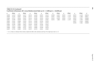
WINDWARD SNOW DRIFT ON LOWER ROOF OF ATTACHED STRUCTURE
In Figure 3.5, if hc/hb is less than 0.2, the drift load is not applied. The drift is given by a triangle
similar to the one shown in Figure 3.6. However, the value of hd is replaced by the following:
0.75[0.43( ) ( 10) 1.5]
1 3 1 4
h L p
d L g
= + − (3.15)
where LL is lower roof length as shown in Figure 3.5.
Equations 3.12 and 3.13 apply to windward width also.
The larger of the values of the leeward and windward heights, hd, from Leeward Snow Drift and
Windward Snow Drift sections is used in the design.
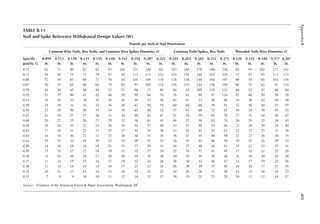
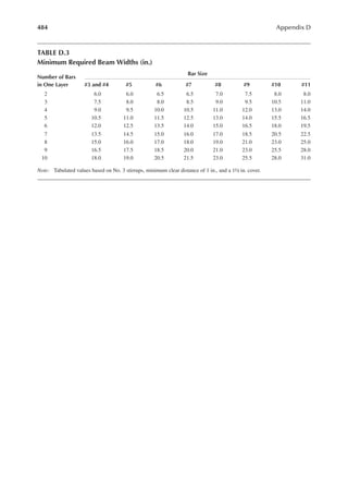
hc
pd = γhd
Lu
hb
hd
w
FIGURE 3.6 Coniguration of snow drift.

60. 42 Principles of Structural Design
LEEWARD SNOW DRIFT ON LOWER ROOF OF SEPARATED STRUCTURE
If the vertical separation distance between the edge of the higher roof including any parapet and the
edge of the adjacent lower roof excluding any parapet is h, and the horizontal separation between
the edges of the two adjacent buildings is s, then the leeward drift to the lower roof is applicable if
the following two conditions are satisied:
1. The horizontal distance, s, is less than 20 ft.
2. The horizontal distance, s, is less than six times the vertical distance, h (s ≤ 6h).
In such a case, the height of the snow drift is the smaller of the following:
1. hd as calculated by Equation 3.10 based on the length of the higher structure
2. 6
6
h s)
( −
The horizontal extent, w, is the smaller of the following:
1. 6hd
2. h s
6 –
( )
WINDWARD SNOW DRIFT ON LOWER ROOF OF SEPARATED STRUCTURE
The same equations as for the windward drift on an attached structure, that is, Equation 3.15 for hd
and Equation 3.12 or 3.13 for w are used. However, the portion of the drift between the edges of the
two adjacent roofs is truncated.
Example 3.5
A two-story residential building has an attached garage, as shown in Figure 3.7. The residential
part is heated and has a well-insulated, ventilated roof, whereas the garage is unheated. Both roofs
of 4 on 12 slope have metal surfaces consisting of the purlins spanning eave to ridge.
The site is a forested area in a small clearing among huge trees. The ground snow load is 40 psf.
Determine the snow load on the lower roof.
30 ft.
60 ft.
Garage
Residence
40 ft.
Roof
Roof
16 ft.
6.67 ft.
4 ft.
8 ft.
24 ft.
FIGURE 3.7 Higher–lower roof drift.

61. 43
Snow Loads
SOLUTION
1. The upper roof is subjected to the balanced snow load and the unbalanced across the ridge
load due to wind in the transverse direction.
2. The lower roof is subjected to the balanced snow load, the unbalanced across the ridge
load due to transverse directional wind, and the drift load from upper to lower roof due to
longitudinal direction wind. Only the lower roof is analyzed here.
3. For the lower roof, the balanced load
a. Unheated roof, Ct = 1.2
b. Residential facility, I = 1.0
c. Terrain B, sheltered, Ce = 1.2
d. 4 on 12 slope, θ = 18.43°
e. For slippery unobstructed surface at Ct = 1.2, from Table 3.4
= −
θ −
= −
−
=
1
( 15)
55
1
(18.43 15)
55
0.94
Cs
f. =
= =
0.7
0.7(0.94)(1.2)(1.2)(1)(40) 37.90 lb/ft.2
p C C C Ip
s s e t g
4. For the lower roof, across the ridge unbalanced load
a. W = 12 < 20 ft., roof rafter system, the simple case applies
b. Windward side no snow load
c. Leeward side
= = =
1
(40) 40 psf
p Ip
u g
5. For lower roof, upper–lower roof drift snow load
a. From Equation 3.8
γ = + = + =
0.13 14 0.13(40) 14 19.2 lb/ft.3
pg
b. =
γ
= =
37.9
19.2
1.97 ft.
h
p
b
s
c. hc = (22.67 − 12) − 1.97 = 8.7 ft.
= = >
8.7
1.97
4.4 0.2 drift load to be considered
h
h
c
b
d. Leeward drift
From Equation 3.10
= + −
= + − =
0.43( ) ( 10) 1.5
0.43(60) (40 10) 1.5 2.97
1 3 1 4
1 3 1 4
h L p
d u g
Since hc > hd, hd = 2.97 ft.
e. pd = γhd = (19.2)(2.97) = 57.03 lb/ft.2
f. From Equation 3.12
= = =
4 4(2.97) 11.88 ft.
w hd

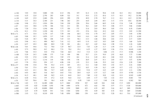
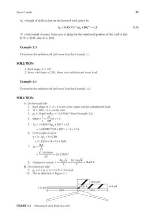
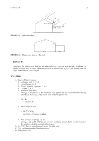
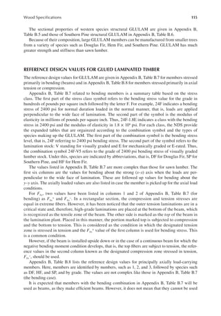
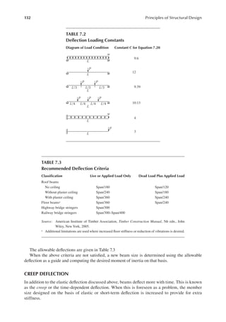
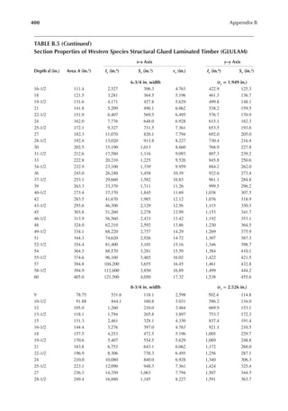
62. 44 Principles of Structural Design
g. Windward drift
= + −
= + −
= <
0.75[0.43( ) ( 10) 1.5]
0.75[0.43(30) (40 10) 1.5]
1.54ft. 2.97ft., leewardcontrols
1 3 1 4
1 3 1 4
h L p
d L g
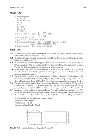
6. Figure 3.8 presents the three loading cases for the lower roof.
SLIDING SNOW LOAD ON LOWER ROOF
A sliding snow load from an upper to a lower roof is superimposed on the balanced snow load. It
is not used in combination with partial, unbalanced, drift, or rain-on-snow loads. The sliding load
(plus the balanced load) and the lower roof drift load (plus the balanced load) are considered as two
separate cases and the higher one is used. One basic difference between a slide and a drift is that in
the former case, snow slides off the upper roof along the slope by the action of gravity and the lower
roof should be in front of the sloping surface to capture this load. In the latter case, wind carries
the snow downstream and thus the drift can take place lengthwise perpendicular to the roof slope,
as in Example 3.5.
The sliding snow load is applied to the lower roof when the upper slippery roof has a slope of
more than θ = 2.4° (1/4 on 12) or when the nonslippery upper roof has a slope greater than 9.5°
(2 on 12).
With reference to Figure 3.9, the total sliding load per unit distance (length) of eave is taken as
0.4 pfW, which is uniformly distributed over a maximum lower roof width of 15 ft. If the width of
the lower roof is less than 15 ft., the sliding load is reduced proportionately. The effect is that it is
equivalent to distribution over a 15 ft. width.
Thus,
0.4
15
p
p W
SL
f
= (3.16)
where
pf is lat upper roof snow load (psf) from Equation 3.1
W is horizontal distance from ridge to eave of the upper roof
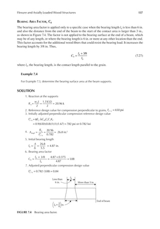
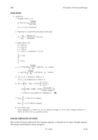
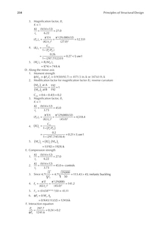
12 ft.
Windward Leeward
Upper to lower roof drift surcharge
12 ft.
11.88 ft.
57.03 psf
12 ft. 12 ft.
37.9 psf (Balanced snow load)
37.9 psf (Balanced snow load)
40 psf (Across the ridge unbalanced snow load)
FIGURE 3.8 Loading on a lower roof.

63. 45
Snow Loads
Example 3.6
Determine the sliding snow load on an unheated lat roof garage attached to a residence, as
shown in Figure 3.10. It is in a suburban area with scattered trees. pg = 20 psf. Assume that the
upper roof lat snow load is 18 psf.
SOLUTION
A. Balanced load on garage
1. Unheated roof, Ct = 1.2
2. Normal usage, I = 1
3. Terrain B, partial exposure, Ce = 1
4. Flat roof, Cs = 1
5. Minimum snow load
Since pg = 20 and θ = 0, the minimum load applies but it is not combined with any
other types (balanced, unbalanced, drift, and sliding) of loads.
=
= =
(1)(20) 20
p Ip
m g
6. Balanced snow load
=
= =
0.7
0.7(1)(1)(1.2)(1)(20) 16.8 lb/ft.2
p C C C Ip
s s e t g
7. Rain-on-snow surcharge = 5 psf
Since pg = 20 and θ < W/50, rain-on-snow surcharge applies, but it is not included in
the unbalanced, drift, and sliding load cases.
B. θ < 2.38°; there is no unbalanced across the ridge load.
C. Drift load not considered in this problem.
D. Sliding snow load
15 ft. max
1 ft.
1 ft.
W
FIGURE 3.9 Sliding snow load.
12
3
4 ft.
40 ft. 18 ft.
FIGURE 3.10 Sliding snow load on a lat roof.

64. 46 Principles of Structural Design
1. Upper roof slope θ = 14° > 9.5°, sliding applies
2. pf = 18 lb/ft.2 (given)
3. = = =
0.4
15
(0.4)(18)(20)
15
9.6 psf
p
p W
SL
f
Figure 3.11 presents the loading cases for the garage.
SLIDING SNOW LOAD ON SEPARATED STRUCTURES
The lower separated roof is subjected to a truncated sliding load if the following two conditions are
satisied:
1. The separation distance between the structures, s, is less than 15 ft.
2. The vertical distance between the structures, h, is greater than the horizontal distance, s
h s)
( >
The sliding load per unit area, pSL, is the same as given by Equation 3.16 but the horizontal extent
on the lower roof is (15 – s). Thus, the load per unit length is
0.4 (15 )
15
S
p W s
L
f
=
−
(3.17)
PROBLEMS
3.1 Determine the balanced snow load on the residential structure shown in Figure P3.1 in a sub-
urban area. The roof is well insulated and ventilated. There are a few trees behind the building
to create obstruction. The ground snow load is 20 lb/ft.2
18 ft.
(a)
16.8 psf (Balanced snow load)
5 psf (Rain-on-snow surcharge)
18 ft.
15 ft.
(b)
16.8 psf (Balanced snow load)
9.6 psf (Sliding snow load)
FIGURE 3.11 Loading on lower roof. (a) Balanced snow load and (b) balanced plus sliding snow load.
12
1/2
130 ft.
130 ft.
FIGURE P3.1 Suburban residence for Problem 3.1.

65. 47
Snow Loads
3.2 Solve Problem 3.1 except that the eave-to-ridge distance is 30 ft.
3.3 Consider a heated warm roof structure in an urban area surrounded by obstructions from all
sides. The eave-to-ridge distance is 25 ft. and the roof height is 7 ft. The ground snow load is
30 psf. Determine the balanced snow load.
3.4 The roof of a high occupancy structure is insulated and well ventilated in a fully open coun-
tryside. The eave-to-ridge distance is 20 ft. and the roof height is 4 ft. The ground snow load
is 25 psf. Determine the balanced snow load.
3.5 Determine the unbalanced load for Problem 3.1.
3.6 Determine the unbalanced load for Problem 3.2.
3.7 Determine the unbalanced snow load for Problem 3.3.
3.8 Determine the unbalanced snow load for Problem 3.4.
3.9 Determine snow load on the lower roof of a building where the ground snow load is 30 lb/ft.2
The elevation difference between the roofs is 5 ft. The higher roof is 70 ft. wide and 100 ft.
long. It is a heated and unventilated ofice building. The lower roof is 60 ft. wide and 100 ft.
long. It is an unheated storage area. Both roofs have 5 on 12 slope of metallic surfaces without
any obstructions. The building is located in an open country with no obstructions. The build-
ing is laid out lengthwise, as shown in Figure P3.2.
3.10 Solve Problem 3.9 except that the roofs’ elevation difference is 3 ft.
3.11 Solve Problem 3.9 when the building is laid out side by side, as shown in Figure P3.3. The lowest
roof is lat.
3.12 Solve Problem 3.9. The two roofs are separated by a horizontal distance of 15 ft.
3.13 Solve Problem 3.11. The two roofs are separated by a horizontal distance of 10 ft.
3.14 Solve Problem 3.11 for the sliding snow load.
100 ft.
100 ft.
Roof
5
on
12
Roof
5
on
12
70 ft. 60 ft.
FIGURE P3.2 Different level roofs lengthwise for Problem 3.9.
100 ft.
60 ft.
70 ft.
Roof
5
on
12
FIGURE P3.3 Different level roofs side by side for Problem 3.11.

66. 48 Principles of Structural Design
3.15 Determine the snow load due to sliding effect for a heated storage area attached to an ofice
building with a well-ventilated/insulated roof in an urban area in Rhode Island having scat-
tered obstructions, as shown in Figure P3.4.
3.16 Determine the sliding load for an unheated garage attached to a cooled roof of a residence
shown in Figure P3.5 in a partially exposed suburban area. The ground snow load is 15 lb/ft.2
3.17 Solve Problem 3.15. The two roofs are separated by a horizontal distance of 2 ft.
3.18 Solve Problem 3.16. The two roofs are separated by a horizontal distance of 3 ft.
12
12
2
5 ft.
4
50 ft.
20 ft.
50 ft.
FIGURE P3.4 Sliding snow on urban building for Problem 3.15.
12
12
2
5 ft.
4
40 ft.
12 ft.
FIGURE P3.5 Sliding snow on suburban building for Problem 3.16.

67. 49
4 Wind Loads
INTRODUCTION
ASCE 7-10 has made major revisions to wind load provisions; from one single chapter (Chapter 6)
in ASCE 7-05, six chapters (Chapters 26 through 31) have been incorporated in ASCE 7-10. The
provisions and the data have been revised to relect the strength (load resistance factor design) level
of design.
Two separate categories have been identiied for wind load provisions:
1. Main wind force–resisting system (MWFRS): MWFRS represents the entire structure
comprising an assemblage of the structural elements constituting the structure that can
sustain wind from more than one surface.
2. Components and cladding (C and C): These are the individual elements that face wind
directly and pass on the loads to the MWFRS.
The broad distinction is apparent. The entire lateral force–resisting system as a unit that transfers
loads to the foundation belongs to the irst category. In the second category, the cladding comprises
wall and roof coverings like sheathing and inish material, curtain walls, exterior windows, and
doors. The components include fasteners, purlins, girts, and roof decking.
However, there are certain elements like trusses and studs that are part of the MWFRS but could
also be treated as individual components.
The C and C loads are higher than MWFRS loads since they are developed to represent the peak
gusts over small areas that result from localized funneling and turbulence of wind.
An interpretation has been made that while using MWFRS, the combined interactions of the
axial and bending stresses due to the vertical loading together with the lateral loading should be
used. But in the application of C and C, either the axial or the bending stress should be considered
individually. They are not combined together since the interaction of loads from multiple surfaces
is not intended to be used in C and C.
DEFINITION OF TERMS
1. Low-rise building: An enclosed or partially enclosed building that has a mean roof height
of less than or equal to 60 ft. and the mean roof height does not exceed the least horizontal
dimension.
2. Open, partially enclosed, and enclosed building: An open building has at least 80%
open area in each wall, that is, Ao/Ag ≥ 0.8, where Ao is total area of openings in a wall and
Ag is the total gross area of that wall.
A partially enclosed building complies with both of the two conditions: (1) the total
area of openings in a wall that receives the external positive pressure exceeds the sum of
the areas of openings in the balance of the building including roof by more than 10% and
(2) the total area of openings in a wall that receives the positive external pressure exceeds
4 ft.2 or 1% of the area of that wall, whichever is smaller, and the percentage of openings
in the balance of the building envelope does not exceed 20%.
An enclosed building is one that is not open and that is not partially enclosed.
3. Regular-shaped building: A building not having any unusual irregularity in spatial form.

68. 50 Principles of Structural Design
4. Diaphragm building: Roof, loor, or other membrane or bracing system in a building that
transfers lateral forces to the vertical MWFRS.
5. Hurricane-prone regions: Areas vulnerable to hurricanes comprising (1) the U.S. Atlantic
Ocean and Gulf of Mexico coasts where the basic wind speed is more than 115 miles/h and
(2) Hawaii, Puerto Rico, Guam, Virgin Island, and American Samoa, covered as special
wind regions in basic wind speed maps.
6. Special wind regions: Regions mentioned as item (2) under hurricane-prone regions.
These should be examined for higher local winds.
7. Mean roof height*: The average of the height to the highest point on roof and the eave
height, measured from ground surface. For a roof angle of 10° or less, it is taken to be the
eave height.
PROCEDURES FOR MWFRS
The following procedures have been stipulated for MWFRS in ASCE 7-10:
1. Wind tunnel procedure: This applies to all types of buildings and structures of all heights
as speciied in Chapter 31.
2. Analytical directional procedure: This applies to regular-shaped buildings of all heights as
speciied in Part 1 of Chapter 27.
3. Simpliied directional procedure: This applies to regular-shaped enclosed simple dia-
phragm buildings of 160 ft. or less height as speciied in Part 2 of Chapter 27.
4. Analytical envelope procedure: This applies to regular-shaped low-rise buildings of 60 ft.
or less height as speciied in Part 1 of Chapter 28.
5. Simpliied envelope procedure: This applies to enclosed simple diaphragm low-rise build-
ings of 60 ft. or less height as speciied in Part 2 of Chapter 28. Since this procedure can be
applied to one- and two-story buildings in most locations, it has been adopted in this book.
SIMPLIFIED PROCEDURE FOR MWFRS FOR LOW-RISE BUILDINGS
The following are the steps of the procedure:
1. Determine the basic wind speed, V, corresponding to the risk category of the building from
one of the Figures 4.1 through 4.3.
2. Determine the upwind exposure category depending on the surface roughness that prevails
in the upwind direction of the structure, as indicated in Table 4.1.
3. Determine the height and exposure adjustment coeficient λ from Table 4.2.
4. The topographic factor, Kzt, has to be applied to a structure that is located on an isolated
hill of at least 60 ft. height for exposure B and of at least 15 ft. height for exposures C
and D, and it should be unobstructed by any similar hill for at least a distance of 100 times
the height of the hill or 2 miles, whichever is less, and the hill should also protrude above
the height of upwind terrain features within 2 miles radius by a factor of 2 or more. The
factor is assessed by the three multipliers that are presented in Figure 26.8-1 of ASCE 7-10.
For usual cases, Kzt = 1.
5. Determine ps30 from Table 4.3, reproduced from ASCE 7-10. For roof slopes more than
25° and less than or equal to 45°; check for both load cases 1 and 2 in the table.
* For seismic loads, the height is measured from the base of the structure.

69. 51
Wind Loads
105(47)
110(49)
120(54)
130(58)
140(63)
130(58)
140(63)
130(58)
140(63)
150(67)
160(72)
170(76)
170(76)
140(63)
(m/s)
180 (80)
150 (67)
150 (67)
115 (51)
150(67)
160(72)
Puerto Rico
150(67)
Special wind region
(a)
Location
Guam
Virgin Islands
American Samoa
Hawaii –
140(63)
130(58)
120(54)
110(49)
105(47)
105(47)
Special wind region statewide
Vmph
FIGURE 4.1 Basic wind speed for risk category I buildings. (a) and (b) simply divides the country in two
halves. Notes: 1. Values are nominal design 3-second gust wind speeds in miles per hour (m/s) at 33 ft. (10 m)
above ground for exposure C category. 2. Linear interpolation between contours is permitted. 3. Islands and
coastal areas outside the last contour shall use the last wind speed contour of the coastal area. 4. Mountainous
terrain, gorges, ocean promontories, and special wind regions shall be examined for unusual wind condi-
tions. 5. Wind speeds correspond to approximately a 15% probability of exceedance in 50 years (Annual
Exceedance Probability = 0.00333, MRI = 300 years). (Courtesy of American Society of Civil Engineers.)

70. 52 Principles of Structural Design
100(45)
105(47)
140(63) 130(58)
120(54)
110(49)
105(47)
105(47)
110(49)
120(54)
130(58)
140(63)
150(67)
150(67)
(b)
FIGURE 4.1 (continued) Basic wind speed for risk category I buildings. (a) and (b) simply divides the
country in two halves. Notes: 1. Values are nominal design 3-second gust wind speeds in miles per hour (m/s)
at 33 ft. (10 m) above ground for exposure C category. 2. Linear interpolation between contours is permitted.
3. Islands and coastal areas outside the last contour shall use the last wind speed contour of the coastal
area. 4. Mountainous terrain, gorges, ocean promontories, and special wind regions shall be examined for
unusual wind conditions. 5. Wind speeds correspond to approximately a 15% probability of exceedance in
50 years (Annual Exceedance Probability = 0.00333, MRI = 300 years). (Courtesy of American Society of
Civil Engineers.)

71. 53
Wind Loads
115(51)
120(54)
130(58)
140(63)
150(67)
150(67)
140(63)
140(63)
160(72)
170(76)
180(80)
180(80)
150(67)
(m/s)
195 (87)
165 (74)
160 (72)
130 (58)
170(76)
160(72)
Puerto Rico
160(72)
170(76)
Special wind region
Location
Guam
Virgin Islands
American Samoa
Hawaii –
150(67)
140(63)
130(58)
120(54)
115(51)
115(51)
Special wind region statewide
Vmph
(a)
FIGURE 4.2 Basic wind speed for risk category II buildings. (a) and (b) simply divides the country in two
halves. Notes: 1. Values are nominal design 3-second gust wind speeds in miles per hour (m/s) at 33 ft. (10 m)
above ground for exposure C category. 2. Linear interpolation between contours is permitted. 3. Islands and
coastal areas outside the last contour shall use the last wind speed contour of the coastal area. 4. Mountainous
terrain, gorges, ocean promontories, and special wind regions shall be examined for unusual wind conditions.
5. Wind speeds correspond to approximately a 7% probability of exceedance in 50 years (Annual Exceedance
Probability = 0.00143, MRI = 700 years). (Courtesy of American Society of Civil Engineers.)

72. 54 Principles of Structural Design
110(49)
115(51)
150(67)
140(63) 130(58)
120(54)
110(49)
110(49)
120(54)
130(58)
140(63)
150(67)
160(72)
160(72)
(b)
FIGURE 4.2 (continued) Basic wind speed for risk category II buildings. (a) and (b) simply divides the
country in two halves. Notes: 1. Values are nominal design 3-second gust wind speeds in miles per hour (m/s)
at 33 ft. (10 m) above ground for exposure C category. 2. Linear interpolation between contours is permitted.
3. Islands and coastal areas outside the last contour shall use the last wind speed contour of the coastal
area. 4. Mountainous terrain, gorges, ocean promontories, and special wind regions shall be examined for
unusual wind conditions. 5. Wind speeds correspond to approximately a 7% probability of exceedance in
50 years (Annual Exceedance Probability = 0.00143, MRI = 700 years). (Courtesy of American Society of
Civil Engineers.)

73. 55
Wind Loads
120(54)
130(58)
140(63)
150(67)
160(72)
150(67)
160(72)
150(67)
160(72)
170(76)
180(80)
190(85)
200(89)
200(89)
180(80)
170(76)
160(72)
150(67)
140(63)
130(58)
120(54)
210 (94)
170(76)
160(72)
180(80)
Puerto Rico
Special wind region
Location
Guam
Virgin Islands
American Samoa
Hawaii –
120(54)
Special wind region statewide
175 (78)
170 (76)
145 (65)
Vmph (m/s)
(a)
FIGURE 4.3 Basic wind speed for risk category III and IV buildings. (a) and (b) simply divides the coun-
try in two halves. Notes: 1. Values are nominal design 3-second gust wind speeds in miles per hour (m/s)
at 33 ft. (10 m) above ground for exposure C category. 2. Linear interpolation between contours is permitted.
3. Islands and coastal areas outside the last contour shall use the last wind speed contour of the coastal area.
4. Mountainous terrain, gorges, ocean promontories, and special wind regions shall be examined for unusual
wind conditions. 5. Wind speeds correspond to approximately a 3% probability of exceedance in 50 years
(Annual Exceedance Probability = 0.000588, MRI = 1700 years). (Courtesy of American Society of Civil
Engineers.)

74. 56 Principles of Structural Design
115(52)
120(54)
160(72)
150(67)
140(63) 130(58)
120(54)
115(51)
115(51)
120(54)
130(58)
140(63)
150(67)
165(74)
165(74)
(b)
FIGURE 4.3 (continued) Basic wind speed for risk category III and IV buildings. (a) and (b) simply
divides the country in two halves. Notes: 1. Values are nominal design 3-second gust wind speeds in miles
per hour (m/s) at 33 ft. (10 m) above ground for exposure C category. 2. Linear interpolation between contours
is permitted. 3. Islands and coastal areas outside the last contour shall use the last wind speed contour of the
coastal area. 4. Mountainous terrain, gorges, ocean promontories, and special wind regions shall be examined
for unusual wind conditions. 5. Wind speeds correspond to approximately a 3% probability of exceedance in
50 years (Annual Exceedance Probability = 0.000588, MRI = 1700 years). (Courtesy of American Society of
Civil Engineers.)

75. 57
Wind Loads
6. The combined windward and leeward net wind pressure, ps, is determined by the following
simpliied equation:
30
p K p
s zt s
= λ (4.1)
where
λ is adjustment factor for structure height and exposure (Tables 4.1 and 4.2)
Kzt is topographic factor; for usual cases 1
ps30 is simpliied standard design wind pressure (Table 4.3)
The pressure ps is the pressure that acts horizontally on the vertical and vertically on the horizon-
tal projection of the structure surface. It represents the net pressure that algebraically sums up the
external and internal pressures acting on a building surface. Furthermore in the case of MWFRS,
for the horizontal pressures that act on the building envelope, the ps combines the windward and
leeward pressures.
The plus and minus signs signify the pressures acting toward and away, respectively, from the
projected surface.
HORIZONTAL PRESSURE ZONES FOR MWFRS
The horizontal pressures acting on the vertical plane are separated into the following four pressure
zones, as shown in Figure 4.4:
A: End zone of wall
B: End zone of (vertical projection) roof
C: Interior zone of wall
D: Interior zone of (vertical projection) roof
TABLE 4.1
Exposure Category for Wind Load
Surface Roughness Exposure Category
Urban and suburban areas, wooded areas, closely spaced dwellings B
Scattered obstructions—lat open country, grasslands C
Flat unobstructed areas, smooth mud and salt lats, water surfaces D
TABLE 4.2
Adjustment Factor for Height and Exposure
Exposure
Mean Roof Height (ft.) B C D
15 1.00 1.21 1.47
20 1.00 1.29 1.55
25 1.00 1.35 1.61
30 1.00 1.40 1.66
35 1.05 1.45 1.70
40 1.09 1.49 1.74
45 1.12 1.53 1.78
50 1.16 1.56 1.81
55 1.19 1.59 1.84
60 1.22 1.62 1.87

76. 58
Principles
of
Structural
Design
TABLE 4.3
Simpliied Design Wind Pressure, ps30 (psf)
Basic Wind Speed (mph) Roof Angle (degrees) Load Case
Zones
Horizontal Pressures Vertical Pressures Overhangs
A B C D E F G H EOH GOH
110 0–5 1 19.2 −10.0 12.7 −5.9 −23.1 −13.1 −16.0 −10.1 −32.3 −25.3
10 1 21.6 −9.0 14.4 −5.2 −23.1 −14.1 −16.0 −10.8 −32.3 −25.3
15 1 24.1 −8.0 16.0 −4.6 −23.1 −15.1 −16.0 −11.5 −32.3 −25.3
20 1 26.6 −7.0 17.7 −3.9 −23.1 −16.0 −16.0 −12.2 −32.3 −25.3
25 1 24.1 3.9 17.4 4.0 −10.7 −14.6 −7.7 −11.7 −19.9 −17.0
2 — — — — −4.1 −7.9 −1.1 −5.1 — —
30–45 1 21.6 14.8 17.2 11.8 1.7 −13.1 0.6 −11.3 −7.6 −8.7
2 21.6 14.8 17.2 11.8 8.3 −6.5 7.2 −4.6 −7.6 −8.7
115 0–5 1 21.0 −10.9 13.9 −6.5 −25.2 −14.3 −17.5 −11.1 −35.3 −27.6
10 1 23.7 −9.8 15.7 −5.7 −25.2 −15.4 −17.5 −11.8 −35.3 −27.6
15 1 26.3 −8.7 17.5 −5.0 −25.2 −16.5 −17.5 −12.6 −35.3 −27.6
20 1 29.0 −7.7 19.4 −4.2 −25.2 −17.5 −17.5 −13.3 −35.3 −27.6
25 1 26.3 4.2 19.1 4.3 −11.7 −15.9 −8.5 −12.8 −21.8 −18.5
2 — — — — −4.4 −8.7 −1.2 −5.5 — —
30–45 1 23.6 16.1 18.8 12.9 1.8 −14.3 0.6 −12.3 −8.3 −9.5
2 23.6 16.1 18.8 12.9 9.1 −7.1 7.9 −5.0 −8.3 −9.5
120 0–5 1 22.8 −11.9 15.1 −7.0 −27.4 −15.6 −19.1 −12.1 −38.4 −30.1
10 1 25.8 −10.7 17.1 −6.2 −27.4 −16.8 −19.1 −12.9 −38.4 −30.1
15 1 28.7 −9.5 19.1 −5.4 −27.4 −17.9 −19.1 −13.7 −38.4 −30.1
20 1 31.6 −8.3 21.1 −4.6 −27.4 −19.1 −19.1 −14.5 −38.4 −30.1
25 1 28.6 4.6 20.7 4.7 −12.7 −17.3 −9.2 −13.9 −23.7 −20.2
2 — — — — −4.8 −9.4 −1.3 −6.0 — —
30–45 1 25.7 17.6 20.4 14.0 2.0 −15.6 0.7 −13.4 −9.0 −10.3
2 25.7 17.6 20.4 14.0 9.9 −7.7 8.6 −5.5 −9.0 −10.3

77. 59
Wind
Loads
130 0–5 1 26.8 −13.9 17.8 −8.2 −32.2 −18.3 −22.4 −14.2 −45.1 −35.3
10 1 30.2 −12.5 20.1 −7.3 −32.2 −19.7 −22.4 −15.1 −45.1 −35.3
15 1 33.7 −11.2 22.4 −6.4 −32.2 −21.0 −22.4 −16.1 −45.1 −35.3
20 1 37.1 −9.8 24.7 −5.4 −32.2 −22.4 −22.4 −17.0 −45.1 −35.3
25 1 33.6 5.4 24.3 5.5 −14.9 −20.4 −10.8 −16.4 −27.8 −23.7
2 — — — — −5.7 −11.1 −1.5 −7.1 — —
30–45 1 30.1 20.6 24.0 16.5 2.3 −18.3 0.8 −15.7 −10.6 −12.1
2 30.1 20.6 24.0 16.5 11.6 −9.0 10.0 −6.4 −10.6 −12.1
140 0–5 1 31.1 −16.1 20.6 −9.6 −37.3 −21.2 −26.0 −16.4 −52.3 −40.9
10 1 35.1 −14.5 23.3 −8.5 −37.3 −22.8 −26.0 −17.5 −52.3 −40.9
15 1 39.0 −12.9 26.0 −7.4 −37.3 −24.4 −26.0 −18.6 −52.3 −40.9
20 1 43.0 −11.4 28.7 −6.3 −37.3 −26.0 −26.0 −19.7 −52.3 −40.9
25 1 39.0 6.3 28.2 6.4 −17.3 −23.6 −12.5 −19.0 −32.3 −27.5
2 — — — — −6.6 −12.8 −1.8 −8.2 — —
30–45 1 35.0 23.9 27.8 19.1 2.7 −21.2 0.9 −18.2 −12.3 −14.0
2 35.0 23.9 27.8 19.1 13.4 −10.5 11.7 −7.5 −12.3 −14.0
150 0–5 1 35.7 −18.5 23.7 −11.0 −42.9 −24.4 −29.8 −18.9 −60.0 −47.0
10 1 40.2 −16.7 26.8 −9.7 −42.9 −26.2 −29.8 −20.1 −60.0 −47.0
15 1 44.8 −14.9 29.8 −8.5 −42.9 −28.0 −29.8 −21.4 −60.0 −47.0
20 1 49.4 −13.0 32.9 −7.2 −42.9 −29.8 −29.8 −22.6 −60.0 −47.0
25 1 44.8 7.2 32.4 7.4 −19.9 −27.1 −14.4 −21.8 −37.0 −31.6
2 — — — — −7.5 −14.7 −2.1 −9.4 — —
30–45 1 40.1 27.4 31.9 22.0 3.1 −24.4 1.0 −20.9 −14.1 −16.1
2 40.1 27.4 31.9 22.0 15.4 −12.0 13.4 −8.6 −14.1 −16.1
160 0–5 1 40.6 −21.1 26.9 −12.5 −48.8 −27.7 −34.0 −21.5 −68.3 −53.5
10 1 45.8 −19.0 30.4 −11.1 −48.8 −29.8 −34.0 −22.9 −68.3 −53.5
15 1 51.0 −16.9 34.0 −9.6 −48.8 −31.9 −34.0 −24.3 −68.3 −53.5
20 1 56.2 −14.8 37.5 −8.2 −48.8 −34.0 −34.0 −25.8 −68.3 −53.5
25 1 50.9 8.2 36.9 8.4 −22.6 −30.8 −16.4 −24.8 −42.1 −35.9
2 — — — — −8.6 −16.8 −2.3 −10.7 — —
30–45 1 45.7 31.2 36.3 25.0 3.5 −27.7 1.2 −23.8 −16.0 −18.3
1 45.7 31.2 36.3 25.0 17.6 −13.7 15.2 −9.8 −16.0 −18.3
(Continued)

78. 60
Principles
of
Structural
Design
TABLE 4.3 (continued)
Simpliied Design Wind Pressure, ps30 (psf)
Basic Wind Speed (mph) Roof Angle (degrees) Load Case
Zones
Horizontal Pressures Vertical Pressures Overhangs
A B C D E F G H EOH GOH
180 0–5 1 51.4 −26.7 34.1 −15.8 −61.7 −35.1 −43.0 −27.2 −86.4 −67.7
10 1 58.0 −24.0 38.5 −14.0 −61.7 −37.7 −43.0 −29.0 −86.4 −67.7
15 1 64.5 −21.4 43.0 −12.2 −61.7 −40.3 −43.0 −30.8 −86.4 −67.7
20 1 71.1 −18.8 47.4 −10.4 −61.7 −43.0 −43.0 −32.6 −86.4 −67.7
25 1 64.5 10.4 46.7 10.6 −28.6 −39.0 −20.7 −31.4 −53.3 −45.4
2 — — — — −10.9 −21.2 −3.0 −13.6 — —
30–45 1 57.8 39.5 45.9 31.6 4.4 −35.1 1.5 −30.1 −20.3 −23.2
2 57.8 39.5 45.9 31.6 22.2 −17.3 19.3 −12.3 −20.3 −23.2
200 0–5 1 63.4 −32.9 42.1 −19.5 −76.2 −43.3 −53.1 −33.5 −106.7 −83.5
10 1 71.5 −29.7 47.6 −17.3 −76.2 −46.5 −53.1 −35.8 −106.7 −83.5
15 1 79.7 −26.4 53.1 −15.0 −76.2 −49.8 −53.1 −38.0 −106.7 −83.5
20 1 87.8 −23.2 58.5 −12.8 −76.2 −53.1 −53.1 −40.2 −106.7 −83.5
25 1 79.6 12.8 57.6 13.1 −35.4 −48.2 −25.6 −38.7 −65.9 −56.1
2 — — — — −13.4 −26.2 −3.7 −16.8 — —
30–45 1 71.3 48.8 56.7 39.0 5.5 −43.3 1.8 −37.2 −25.0 −28.7
2 71.3 48.8 56.7 39.0 27.4 −21.3 23.8 −15.2 −25.0 −28.7

79. 61
Wind Loads
The dimension of the end zones A and B are taken equal to 2a, where the value of a is smaller
than the following two values:
1. 0.1 times the least horizontal dimension
2. 0.4 times the roof height, h
The height, h, is the mean height of roof from the ground. For roof angle <10°, it is the height to
the eave.
If the pressure in zone B or D is negative, treat it as zero in computing the total horizontal
force.
For Case B in Figure 4.4, wind acting in the longitudinal direction (wind acting on width),
use θ = 0 and zones B and D do not exist.
VERTICAL PRESSURE ZONES FOR MWFRS
The vertical pressures on the roof are likewise separated into the following four zones, as shown in
Figure 4.5.
E: End zone of (horizontal projection) windward roof
F: End zone of (horizontal projection) leeward roof
G: Interior zone of (horizontal projection) windward roof
H: Interior zone of (horizontal projection) leeward roof
Where the end zones E and G fall on a roof overhang, the pressure values under the columns EOH
and GOH in Table 4.3 are used for the windward side. For the leeward side, the basic values are used.
The dimension of the end zones E and F is taken to be the horizontal distance from edge to ridge
and equal to 2a in windward direction, as shown in Figure 4.5 for both Case A, transverse direc-
tion, and Case B, longitudinal direction. For the longitudinal wind direction, roof angle = 0 is used.
MINIMUM PRESSURE FOR MWFRS
The minimum wind load computed for MWFRS is based on pressures of 16 psf for zones A and B
and pressures of 8 psf for zones B and D, while assuming the pressures for zones E, F, G, and H are
equal to zero.
Eave
height
Reference
center
M
W
FRS direction
Case B: Longitudinal
Reference
center
A
θ
θ
Case A: Transverse
MWFRS direction
A
C C
D
B
2a
2a
FIGURE 4.4 Horizontal pressure zones.

80. 62 Principles of Structural Design
Example 4.1
A two-story essential facility shown in Figure 4.6 is an enclosed wood-frame building located in
Seattle, Washington. Determine the design wind pressures for MWFRS in both principal directions
of the building and the forces acting on the transverse section of the building. The wall studs and
roof rafters are 16 in. on center. Kzt = 1.0.
SOLUTION
I. Design parameters
1. Roof slope, θ = 14°
2. hmean 22
6.25
2
25.13 ft.
= + =
3. End zone dimension, a, smaller than
a. 0.4 hmean = 0.4 (25.13) = 10 ft.
b. 0.1 width = 0.1(50) = 5 ft. ← controls
4. Length of end zone = 2a = 10 ft.
12
3
6.25 ft.
11 ft.
11 ft.
50 ft.
100 ft.
FIGURE 4.6 Two-story framed building.
θ
G
H
F
E
2a
MWFRS direction
Both transverse and longitudinal
M
W
FRS direction
FIGURE 4.5 Vertical pressure zones.

81. 63
Wind Loads
5. Basic wind speed, V = 115 mph
6. Exposure category = B
7. λ from Table 4.3 up to 30 ft. = 1.0
8. Kzt = 1.00 (given)
9. ps = λKzt ps30 = (1)(1)ps30 = ps30
II. Case A: For transverse wind direction
A.1 Horizontal wind pressure on wall and roof projection
A.2 Horizontal force at the roof level
A.3 Horizontal force at the second loor level
Total horizontal force is 39,610. The application of the forces is shown in Figure 4.7b.
B.1 Vertical wind pressure on the roof
Zone
Pressure (psf) (Table 4.3)
ps = ps30 (psf)
Roof Angle = 10° Roof Angle = 15° Interpolated to 14°
E: End, windward −25.2 −25.2 −25.2 −25.2
F: End, leeward −15.4 −16.5 −16.28 −16.28
G: Interior, windward −17.5 −17.5 −17.5 −17.5
H: Interior, leeward −11.6 −12.6 −12.4 −12.4
Note: The pressures are shown in the sectional view in Figure 4.8a.
Tributary
Location Zone Height (ft.) Width (ft.) Area (ft.2) Pressure (psf) Load (lb)
End A 11 10 110 25.78 2,836
Interior C 11 90 990 17.14 16,969
Total 19,805
Location Zone
Tributary
Pressure (psf) Load (lb)
Height (ft.) Width (ft.) Area (ft.2)
End A 11a
2a = 10 110 25.78 2,836
B 6.25 10 62.5 −8.92 → 0 0
Interior C 11 L − 2a = 90 990 17.14 16,969
D 6.25 90 562.5 −5.14 → 0 0
Total 19,805
Note: Taking pressures in zones B and D to be zero.
a It is also a practice to take 1/2 of the loor height for each level. In such a case, the wind force on the 1/2 of
the irst loor height from the ground is not applied.
Zone
Pressure (psf) (Table 4.3)
ps = ps30 (psf)
Roof Angle = 10° Roof Angle = 15° Interpolated for 14°
A. End zone wall 23.7 26.3 25.78 25.78
B. End zone roof −9.8 −8.7 −8.92 −8.92
C. Interior wall 15.7 17.5 17.14 17.14
D. Interior roof −5.7 −5.0 −5.14 −5.14
Note: These pressures are shown in the section view in Figure 4.7a.

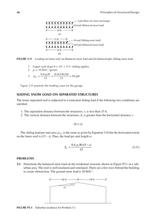
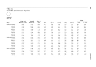
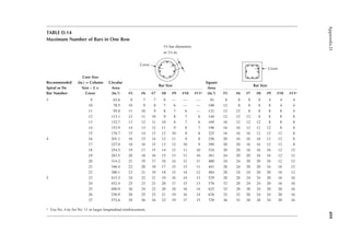
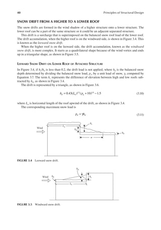
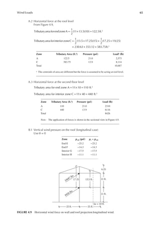
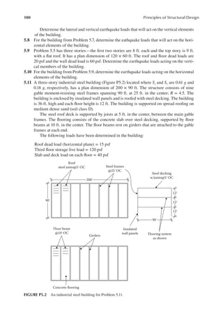
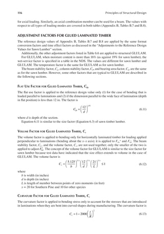
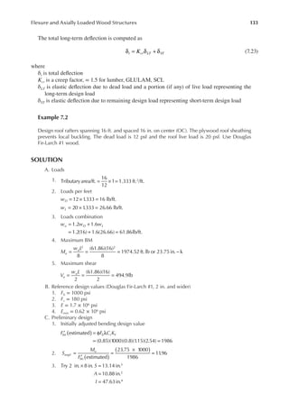
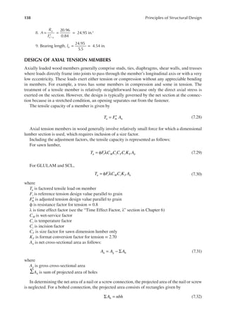
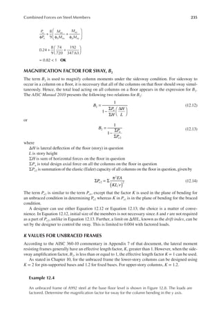
82. 64 Principles of Structural Design
B.2 Vertical force on the roof
C. Minimum force on MWFRS by transverse wind
The minimum pressure is 16 psf acting on the vertical projection of wall and 8 psf on
vertical projection of roof. Thus,
Minimum wind force = [16(22) + 8(6.25)] × 100 = 40,200 lb
D. Applicable wind force
The following two cases should be considered for maximum effect:
1. The combined A.2, A.3, and B.2
2. Minimum force C
III. Case B: For longitudinal wind direction
A.1 Horizontal wind pressures on wall
Zones B and D do not exist. Using θ = 0, pressure on zone A = 21.0 psf and pressure
on zone C = 13.9 psf from Table 4.3.
(b)
Wind direction
–45675 lbs –31970 lbs
(a)
Interior
End
–17.5 psf
–12.4 psf
–16.25 psf
–25.2 psf
FIGURE 4.8 (a) Vertical pressure distribution on roof and (b) vertical force on roof:transverse wind.
Zone
Tributary
Pressure (psf) Load (lb)
Length (ft.) Width (ft.) Area (ft.2)
Windward E: End 25 2a = 10 250 −25.2 −6,300
G: Interior 25 L − 2a = 90 2250 −17.5 −39,375
Total −45,675
Leeward F: End 25 10 250 −16.28 −4,070
H: Interior 25 90 2250 −12.4 −27,900
Total −31,970
Note: The application of vertical forces is shown in Figure 4.8b.
Tributary
Tributary
19805 lbs
17.14 psf
Interior zone
25.78 psf
End zone
–8.92 psf
Wind direction
–5.14 psf
(b)
(a)
19805 lbs
FIGURE 4.7 (a) Horizontal pressure distribution and (b) horizontal force:transverse wind.

83. 65
Wind Loads
A.2 Horizontal force at the roof level
From Figure 4.9,
= + =
TributaryareaforendzoneA
1
2
(11 13.5)(10) 122.5ft.2
= + + +
= + =
TributaryareaforinteriorzoneC
1
2
(13.5 17.25)(15)
1
2
(17.25 11)(25)
230.63 353.12 583.75ft.2
A.3 Horizontal force at the second loor level
Tributary area for end zone A 11 10 110 ft.2
= × =
Tributary area for interior zone C 11 40 440 ft.2
= × =
B.1 Vertical wind pressure on the roof (longitudinal case)
Use θ = 0
Zone Tributary Area (ft.2) Pressure (psf) Load (lb)
A 110 21.0 2310
C 440 13.9 6116
Total 8426
Note: The application of forces is shown in the sectional view in Figure 4.9.
Zone ps30 (psf) ps = ps30
End E −25.2 −25.2
End F −14.3 −14.3
Interior G −17.5 −17.5
Interior H −11.1 −11.1
Zone Tributary Area (ft.2) Pressure (psf) Loada (lb)
A 122.5 21.0 2,573
C 583.75 13.9 8,114
Total 10,687
a The centroids of area are different but the force is assumed to be acting at roof level.
17.25
25 ft. 25 ft.
13.5 ft. 11 ft.
11 ft.
2a = 10 ft.
6.25
10687 lbs
8426 lbs
FIGURE 4.9 Horizontal wind force on wall and roof projection:longitudinal wind.

84. 66 Principles of Structural Design
B.2 Vertical force on the roof
PROCEDURES FOR COMPONENTS AND CLADDING
ASCE 7-10 stipulates that when the tributary area is greater than 700 ft.2, the C and C elements
can be designed using the provisions of MWFRS. Chapter 30 of ASCE 7-10 speciies procedures
for C and C; these are parallel to the procedures of MWFRS. Two analytical procedures—one for
high-rise buildings and one for low-rise buildings—use equations similar to the analytical proce-
dures of MWFRS. Two simpliied procedures—one for regular-shaped enclosed buildings up to
160 ft. in height and one for regular-shaped enclosed low-rise buildings—determine wind pressures
directly from tables. ASCE 7-10 also covers the C and C for open buildings and appurtenances.
SIMPLIFIED PROCEDURE FOR COMPONENTS AND
CLADDING FOR LOW-RISE BUILDINGS
The C and C cover the individual structural elements that directly support a tributary area against the
wind force. The conditions and the steps of the procedure are essentially similar to the MWFRS. The
pressure, however, acts normal to each surface, that is, horizontal on the wall and perpendicular to
the roof. The following similar equation is used to determine the wind pressure. The adjustment fac-
tor, λ, and the topographic factor, Kzt, are determined from the similar considerations as for MWFRS:
p K p
net zt net30
= λ (4.2)
where
λ is adjustment factor for structure height and exposure (Tables 4.1 and 4.2)
Kzt is topographic factor
pnet30 is simpliied standard design wind pressure (Table 4.4)
However, the pressures pnet30 are different from ps30. Besides the basic wind speed, the pressures
are a function of the roof angle, the effective wind area supported by the element, and the zone of
the structure surface. pnet represents the net pressures, which are the algebraic summation of the
internal and external pressures acting normal to the surface of the C and C.
Eave height
90 ft.
10 ft.
9875 64350
FIGURE 4.10 Force on roof:longitudinal wind.
Zone
Tributary
Pressure (psf) Load (lb)
Length (ft.) Width (ft.) Area (ft.2)
End E 2a = 10 B/2 = 25 250 −25.2 −6,300
F 2a = 10 25 250 −14.3 −3,575
Total −9,875
Interior G L −2a = 90 25 2250 −17.5 −39,375
H 90 25 2250 −11.1 −24,975
Total −64,350
Note: The application of forces is shown in Figure 4.10.

85. 67
Wind
Loads
TABLE 4.4
Net Design Wind Pressure, pnet30 (psf)
Zone
Effective
Wind
Area (sf)
Basic Wind Speed V (mph)
110 115 120 130 140 150 160 180 200
Roof 0°–7° 1 10 8.9 −21.8 9.7 −23.8 10.5 −25.9 12.4 −30.4 14.3 −35.3 16.5 −40.5 18.7 −46.1 23.7 −58.3 29.3 −72.0
1 20 8.3 −21.2 9.1 −23.2 9.9 −25.2 11.6 −29.6 13.4 −34.4 15.4 −39.4 17.6 −44.9 22.2 −56.8 27.4 −70.1
1 50 7.6 −20.5 8.3 −22.4 9.0 −24.4 10.6 −28.6 12.3 −33.2 14.1 −38.1 16.0 −43.3 20.3 −54.8 25.0 −67.7
1 100 7.0 −19.9 7.7 −21.8 8.3 −23.7 9.8 −27.8 11.4 −32.3 13.0 −37.0 14.8 −42.1 18.8 −53.3 23.2 −65.9
2 10 8.9 −36.5 9.7 −39.9 10.5 −43.5 12.4 −51.0 14.3 −59.2 16.5 −67.9 18.7 −77.3 23.7 −97.8 29.3 −120.7
2 20 8.3 −32.6 9.1 −35.7 9.9 −38.8 11.6 −45.6 13.4 −52.9 15.4 −60.7 17.6 −69.0 22.2 −87.4 27.4 −107.9
2 50 7.6 −27.5 8.3 −30.1 9.0 −32.7 10.6 −38.4 12.3 −44.5 14.1 −51.1 16.0 −58.2 20.3 −73.6 25.0 −90.9
2 100 7.0 −23.6 7.7 −25.8 8.3 −28.1 9.8 −33.0 11.4 −38.2 13.0 −43.9 14.8 −50.0 18.8 −63.2 23.2 −78.1
3 10 8.9 −55.0 9.7 −60.1 10.5 −65.4 12.4 −76.8 14.3 −89.0 16.5 −102.2 18.7 −116.3 23.7 −147.2 29.3 −181.7
3 20 8.3 −45.5 9.1 −49.8 9.9 −54.2 11.6 −63.6 13.4 −73.8 15.4 −84.7 17.6 −96.3 22.2 −121.9 27.4 −150.5
3 50 7.6 −33.1 8.3 −36.1 9.0 −39.3 10.6 −46.2 12.3 −53.5 14.1 −61.5 16.0 −69.9 20.3 −88.5 25.0 −109.3
3 100 7.0 −23.6 7.7 −25.8 8.3 −28.1 9.8 −33.0 11.4 −38.2 13.0 −43.9 14.8 −50.0 18.8 −63.2 23.2 −78.1
Roof >7°–27° 1 10 12.5 −19.9 13.7 −21.8 14.9 −23.7 17.5 −27.8 20.3 −32.3 23.3 −37.0 26.5 −42.1 33.6 −53.3 41.5 −65.9
1 20 11.4 −19.4 12.5 −21.2 13.6 −23.0 16.0 −27.0 18.5 −31.4 21.3 −36.0 24.2 −41.0 30.6 −51.9 37.8 −64.0
1 50 10.0 −18.6 10.9 −20.4 11.9 −22.2 13.9 −26.0 16.1 −30.2 18.5 −34.6 21.1 −39.4 26.7 −49.9 32.9 −61.6
1 100 8.9 −18.1 9.7 −19.8 10.5 −21.5 12.4 −25.2 14.3 −29.3 16.5 −33.6 18.7 −38.2 23.7 −48.4 29.3 −59.8
2 10 12.5 −34.7 13.7 −37.9 14.9 −41.3 17.5 −48.4 20.3 −56.2 23.3 −64.5 26.5 −73.4 33.6 −92.9 41.5 −114.6
2 20 11.4 −31.9 12.5 −34.9 13.6 −38.0 16.0 −44.6 18.5 −51.7 21.3 −59.3 24.2 −67.5 30.6 −85.4 37.8 −105.5
2 50 10.0 −28.2 10.9 −30.9 11.9 −33.6 13.9 −39.4 16.1 −45.7 18.5 −52.5 21.1 −59.7 26.7 −75.6 32.9 −93.3
2 100 8.9 −25.5 9.7 −27.8 10.5 −30.3 12.4 −35.6 14.3 −41.2 16.5 −47.3 18.7 −53.9 23.7 −68.2 29.3 −84.2
3 10 12.5 −51.3 13.7 −56.0 14.9 −61.0 17.5 −71.6 20.3 −83.1 23.3 −95.4 26.5 −108.5 33.6 −137.3 41.5 −169.5
3 20 11.4 −47.9 12.5 −52.4 13.6 −57.1 16.0 −67.0 18.5 −77.7 21.3 −89.2 24.2 −101.4 30.6 −128.4 37.8 −158.5
3 50 10.0 −43.5 10.9 −47.6 11.9 −51.8 13.9 −60.8 16.1 −70.5 18.5 −81.0 21.1 −92.1 26.7 −116.6 32.9 −143.9
3 100 8.9 −40.2 9.7 −44.0 10.5 −47.9 12.4 −56.2 14.3 −65.1 16.5 −74.8 18.7 −85.1 23.7 −107.7 29.3 −132.9
(Continued)

86. 68
Principles
of
Structural
Design
TABLE 4.4 (continued)
Net Design Wind Pressure, pnet30 (psf)
Zone
Effective
Wind
Area (sf)
Basic Wind Speed V (mph)
110 115 120 130 140 150 160 180 200
Roof >27°–45° 1 10 19.9 −21.8 21.8 −23.8 23.7 −25.9 27.8 −30.4 32.3 −35.3 37.0 −40.5 42.1 −46.1 53.3 −58.3 65.9 −72.0
1 20 19.4 −20.7 21.2 −22.6 23.0 −24.6 27.0 −28.9 31.4 −33.5 36.0 −38.4 41.0 −43.7 51.9 −55.3 64.0 −68.3
1 50 18.6 −19.2 20.4 −21.0 22.2 −22.8 26.0 −26.8 30.2 −31.1 34.6 −35.7 39.4 −40.6 49.9 −51.4 61.6 −63.4
1 100 18.1 −18.1 19.8 −19.8 21.5 −21.5 25.2 −25.2 29.3 −29.3 33.6 −33.6 38.2 −38.2 48.4 −48.4 59.8 −59.8
2 10 19.9 −25.5 21.8 −27.8 23.7 −30.3 27.8 −35.6 32.3 −41.2 37.0 −47.3 42.1 −53.9 53.3 −68.2 65.9 −84.2
2 20 19.4 −24.3 21.2 −26.6 23.0 −29.0 27.0 −34.0 31.4 −39.4 36.0 −45.3 41.0 −51.5 51.9 −65.2 64.0 −80.5
2 50 18.6 −22.9 20.4 −25.0 22.2 −27.2 26.0 −32.0 30.2 −37.1 34.6 −42.5 39.4 −48.4 49.9 −61.3 61.6 −75.6
2 100 18.1 −21.8 19.8 −23.8 21.5 −25.9 25.2 −30.4 29.3 −35.3 33.6 −40.5 38.2 −46.1 48.4 −58.3 59.8 −72.0
3 10 19.9 −25.5 21.8 −27.8 23.7 −30.3 27.8 −35.6 32.3 −41.2 37.0 −47.3 42.1 −53.9 53.3 −68.2 65.9 −84.2
3 20 19.4 −24.3 21.2 −26.6 23.0 −29.0 27.0 −34.0 31.4 −39.4 36.0 −45.3 41.0 −51.5 51.9 −65.2 64.0 −80.5
3 50 18.6 −22.9 20.4 −25.0 22.2 −27.2 26.0 −32.0 30.2 −37.1 34.6 −42.5 39.4 −48.4 49.9 −61.3 61.6 −75.6
3 100 18.1 −21.8 19.8 −23.8 21.5 −25.9 25.2 −30.4 29.3 −35.3 33.6 −40.5 38.2 −46.1 48.4 −58.3 59.8 −72.0
Wall 4 10 21.8 −23.6 23.8 −25.8 25.9 −28.1 30.4 −33.0 35.3 −38.2 40.5 −43.9 46.1 −50.0 58.3 −63.2 72.0 −78.1
4 20 20.8 −22.6 22.7 −24.7 24.7 −26.9 29.0 −31.6 33.7 −36.7 38.7 −42.1 44.0 −47.9 55.7 −60.6 68.7 −74.8
4 50 19.5 −21.3 21.3 −23.3 23.2 −25.4 27.2 −29.8 31.6 −34.6 36.2 −39.7 41.2 −45.1 52.2 −57.1 64.4 −70.5
4 100 18.5 −20.4 20.2 −22.2 22.0 −24.2 25.9 −28.4 30.0 −33.0 34.4 −37.8 39.2 −43.1 49.6 −54.5 61.2 −67.3
4 500 16.2 −18.1 17.7 −19.8 19.3 −21.5 22.7 −25.2 26.3 −29.3 30.2 −33.6 34.3 −38.2 43.5 −48.4 53.7 −59.8
5 10 21.8 −29.1 23.8 −31.9 25.9 −34.7 30.4 −40.7 35.3 −47.2 40.5 −54.2 46.1 −61.7 58.3 −78.0 72.0 −96.3
5 20 20.8 −27.2 22.7 −29.7 24.7 −32.4 29.0 −38.0 33.7 −44.0 38.7 −50.5 44.0 −57.5 55.7 −72.8 68.7 −89.9
5 50 19.5 −24.6 21.3 −26.9 23.2 −29.3 27.2 −34.3 31.6 −39.8 36.2 −45.7 41.2 −52.0 52.2 −65.8 64.4 −81.3
5 100 18.5 −22.6 20.2 −24.7 22.0 −26.9 25.9 −31.6 30.0 −36.7 34.4 −42.1 39.2 −47.9 49.6 −60.6 61.2 −74.8
5 500 16.2 −18.1 17.7 −19.8 19.3 −21.5 22.7 −25.2 26.3 −29.3 30.2 −33.6 34.3 −38.2 43.5 −48.4 53.7 −59.8
Note: For effective areas between those given above the load may be interpolated, otherwise use the load associated with the lower effective area.

87. 69
Wind Loads
The effective area is the tributary area of an element but need not be lesser than the span length
multiplied by the width equal to one-third of the span length, that is, /3
2
A L
= .
Table 4.4, reproduced from ASCE 7-10, lists pnet30 values for effective wind areas of 10, 20, 50,
and 100 ft.2 for roof and additionally 500 ft.2 for wall. A roof element having an effective area in
excess of 100 ft.2 should use pressures corresponding to an area of 100 ft.2 Similarly, a wall element
supporting an area in excess of 500 ft.2 should use pressures corresponding to 500 ft.2 A linear inter-
polation is permitted for intermediate areas. Table 4.5 lists pnet30 values for roof overhang.
The following zones shown in Figure 4.11 have been identiied for the C and C.
The dimension a is smaller than the following two values:
1. 0.4 times the mean height to roof, hmean
2. 0.1 times the smaller horizontal dimension
But, the value of a should not be less than the following:
1. 0.04 times the smaller horizontal dimension
2. 3 ft.
TABLE 4.5
Roof Overhang Net Design Wind Pressure, pnet30 (psf)
Zone
Effective
Wind
Area (sf)
Basic Wind Speed V (mph)
110 115 130 140 150 160 180 200
Roof 0°–7° 2 10 −31.4 −34.3 −43.8 −50.8 −58.3 −66.3 −84.0 −103.7
2 20 −30.8 −33.7 −43.0 −49.9 −57.3 −65.2 −82.5 −101.8
2 50 −30.1 −32.9 −42.0 −48.7 −55.9 −63.6 −80.5 −99.4
2 100 −29.5 −32.3 −41.2 −47.8 −54.9 −62.4 −79.0 −97.6
3 10 −51.6 −56.5 −72.1 −83.7 −96.0 −109.3 −138.3 −170.7
3 20 −40.5 −44.3 −56.6 −65.7 −75.4 −85.8 −108.6 −134.0
3 50 −25.9 −28.3 −36.1 −41.9 −48.1 −54.7 −69.3 −85.5
3 100 −14.8 −16.1 −20.6 −23.9 −27.4 −31.2 −39.5 −48.8
Roof >7°–27° 2 10 −40.6 −44.4 −56.7 −65.7 −75.5 −85.9 −108.7 −134.2
2 20 −40.6 −44.4 −56.7 −65.7 −75.5 −85.9 −108.7 −134.2
2 50 −40.6 −44.4 −56.7 −65.7 −75.5 −85.9 −108.7 −134.2
2 100 −40.6 −44.4 −56.7 −65.7 −75.5 −85.9 −108.7 −134.2
3 10 −68.3 −74.6 −95.3 −110.6 −126.9 −144.4 −182.8 −225.6
3 20 −61.6 −67.3 −86.0 −99.8 −114.5 −130.3 −164.9 −203.6
3 50 −52.8 −57.7 −73.7 −85.5 −98.1 −111.7 −141.3 −174.5
3 100 −46.1 −50.4 −64.4 −74.7 −85.8 −97.6 −123.5 −152.4
Roof >27°–45° 2 10 −36.9 −40.3 −51.5 −59.8 −68.6 −78.1 −98.8 −122.0
2 20 −35.8 −39.1 −50.0 −58.0 −66.5 −75.7 −95.8 −118.3
2 50 −34.3 −37.5 −47.9 −55.6 −63.8 −72.6 −91.9 −113.4
2 100 −33.2 −36.3 −46.4 −53.8 −61.7 −70.2 −88.9 −109.8
3 10 −36.9 −40.3 −51.5 −59.8 −68.6 −78.1 −98.8 −122.0
3 20 −35.8 −39.1 −50.0 −58.0 −66.5 −75.7 −95.8 −118.3
3 50 −34.3 −37.5 −47.9 −55.6 −63.8 −72.6 −91.9 −113.4
3 100 −33.2 −36.3 −46.4 −53.8 −61.7 −70.2 −88.9 −109.8

88. 70 Principles of Structural Design
There are two values of the net pressure that act on each element: a positive pressure acting
inward (toward the surface) and a negative pressure acting outward (away from the surface). The two
pressures must be considered separately for each element.
MINIMUM PRESSURES FOR COMPONENTS AND CLADDING
The positive pressure, pnet, should not be less than +16 psf and the negative pressure should not be
less than −16 psf.
Example 4.2
Determine design wind pressures and forces for the studs and rafters of Example 4.1.
SOLUTION
A. Parameters
1. θ = 14°
2. a = 5 ft. (from Example 4.1), which is more than (1) 0.04 (50) = 2 ft. and (2) 3 ft.
3. pnet = pnet30 (from Example 4.1)
B. Wind pressures on studs (wall) at each loor level
1. Effective area
A L W
= × = × =
11
16
12
14.7ft.2
A
L
min
3
(11)
3
40.3ft.
2 2
2
= = =
2. Net wall pressures for V = 115 mph
Zone
pnet30 at Interpolated
Effective Area 40.3 ft.2 (psf) pnet = pnet30 (psf)
End: 5 21.75 −27.80 21.75 −27.80
Interior: 4 21.75 −23.75 21.75 −23.75
5
4
4
5
5
5
3 2 2 3
2 1 1 2
3 2 2 3
a
a
a
a
θ
a
(a) (b)
Interior zones
Wall
Roof
Wall
Roof
5
2
4
1 3
Roof
Corner zones
End zones
a
h
a
a
FIGURE 4.11 Zones for components and cladding: (a) elevation and (b) plan.

89. 71
Wind Loads
C. Wind forces on studs
C.1 On end studs that have higher pressures
1. Positive W = pnet (tributary area*)
= =
21
.75 (14.7) 319.73 lb (inward)
2. Negative W = pnet (tributary area)
= 27.80 (14.7) = 408.66 lb (outward)
− −
These are shown in Figure 4.12.
D. Wind pressures on rafters (roof)
1. Length of rafter
25
cos14
25.76 ft.
=
°
=
2. A =





 =
(25.76)
16
12
34.35ft.2
3. A
L
min
3
(25.76)
3
221ft. ,use100ft.
2 2
2 2
= = =
4. Net roof pressures at θ between 7° and 27°
E. Wind forces on rafters
E.1 On end rafters
1. pnet
Positive W (tributary area) 16 (34.35) 549.6 lb (inward)
= = =
2. W pnet
Negative (tributary area) 27.8(34.35) 954.9 lb (outward)
= = − = −
3. These are shown in Figure 4.13.
* Use the tributary area not the effective area.
–954.9 lbs
549.6 lbs
25.76 ft.
25.76 ft.
FIGURE 4.13 Wind force on end rafters.
Zone pnet30 at 100 ft.2 (psf) pnet = pnet30 (psf)
Corner 3 9.7 −44.0 9.7a
−44.0
End 2 9.7 −27.8 9.7a
−27.8
Interior 1 9.7 −19.8 9.7a
−19.8
a Use a minimum of 16 psf.
11 ft.
11 ft.
319.73 lbs 408.66 lbs
FIGURE 4.12 Wind force on end studs.

90. 72 Principles of Structural Design
PROBLEMS
4.1 A circular-shaped ofice building is located in downtown Boston, Massachusetts. It has a
height of 160 ft. to which the lateral load is transferred to the MWFRS through the loor and
roof system. The front facing wall that receives the positive external pressure has an area
of 1600 ft.2 of which 400 ft.2 is an open area. The other three side walls have a wall area
of 1600 ft.2 and openings of 100 ft.2 each. Whether it is an open, partial open, or enclosed
building? Which is the most appropriate MWFRS procedure to determine the wind loads?
4.2 A square 100-ft.-high ofice building transfers loads through loors and roof systems to the
walls and foundations. All wall sizes are 1000 ft.2 and there are openings of 200 ft.2 each.
Whether it is a partial open or enclosed building? What is the most appropriate procedure
to determine the wind loads?
4.3 Consider a 100 ft. × 50 ft. ive-story building where the irst three stories are 9 ft. each and
the other two stories are 8 ft. each. It is located in a remote open countryside in Maine, New
England. The roof slope is 8°. Determine the exposure category and the height adjustment
factor.
4.4 Consider a four-story coastal building in Newport, Rhode Island, where the height of each
loor is 12.5 ft. The width of the building is 50 ft. and the roof slope is 14°. Determine the
exposure category and the adjustment factor for height.
4.5 Determine the horizontal wind pressures and forces on the wall and the vertical pressures
and forces acting on the roof due to wind acting in the transverse direction on an MWFRS
as shown in Figure P4.1. It is a standard occupancy single-story building located in an
urban area in Rhode Island where the basic wind speed is 140 mph. Kzt = 1.
4.6 In Problem 4.5, determine the horizontal pressures and forces and the vertical pressures
and forces in the longitudinal direction.
4.7 An enclosed two-story heavily occupied building located in an open, lat terrain in Portland,
Oregon, is shown in Figure P4.2. Determine the wind pressures on the walls and roofs of
the MWFRS in the transverse direction. Also determine the design wind forces in the
transverse direction. Kzt = 1.
100 ft.
50 ft.
50 ft.
14 ft.
7 ft.
FIGURE P4.1 A single-story building in an urban area for Problem 4.5.
80 ft. 40 ft.
40 ft.
10 ft.
9 ft.
4 ft.
FIGURE P4.2 A two-story building in open terrain for Problem 4.7.

91. 73
Wind Loads
4.8 In Problem 4.7, determine the wind pressures and forces on the walls and roof in the longi-
tudinal direction.
4.9 A three-story industrial steel building, shown in Figure P4.3, located in unobstructed ter-
rain in Honolulu, Hawaii, has a plan dimension of 200 ft. × 90 ft. The structure consists of
nine moment-resisting steel frames spanning 90 ft. at 25 ft. in the center. It is roofed with
steel deck, which is pitched at 1.25° on each side from the center. The building is 36 ft. high
with each loor having a height of 12 ft. Determine the MWFRS horizontal and vertical
pressures and the forces due to wind in the transverse direction of the building. Kzt = 1.
4.10 In Problem 4.9, determine the MWFRS horizontal and vertical pressures and the forces in
the longitudinal direction.
4.11 The building in Problem 4.5 has the wall studs and roof trusses spaced at 12 in. in the
center. Determine the elemental wind pressures and forces on the studs and roof trusses.
4.12 The building in Problem 4.7 has the wall studs and roof trusses spaced at 16 in. in the
center. Determine the elemental wind pressures and forces on the studs and roof trusses.
4.13 Determine the wind pressures and forces on the wall panel and roof decking from
Problem 4.9. Decking is supported on joists that are 5 ft. in the center, spanning across the
steel frames shown in Figure P4.3.
200 ft.
90 ft.
Steel frames with steel desk
at 25 ft. in the center
90 ft.
12 ft.
12 ft.
1.25°
12 ft.
FIGURE P4.3 A three-story industrial building for Problem 4.9.

93. 75
5 Earthquake Loads
SEISMIC FORCES
The earth’s outer crust is composed of very big, hard plates as large or larger than a continent.
These plates loat on the molten rock beneath. When these plates encounter each other, appreciable
horizontal and vertical ground motion of the surface occurs known as the earthquake. For example,
in the western portion of the United States, an earthquake is caused by the two plates comprising
the North American continent and the Paciic basin. The ground motion induces a very large inertia
force known as the seismic force in a structure that often results in the destruction of the structure.
The seismic force acts vertically like dead and live loads and laterally like wind load. But unlike the
other forces that are proportional to the exposed area of the structure, the seismic force is propor-
tional to the mass of the structure and is distributed in proportion to the structural mass at various
levels.
In all other types of loads including the wind load, the structural response is static wherein the
structure is subjected to a pressure applied by the load. However, in a seismic load, there is no such
direct applied pressure.
If ground movement could take place slowly, the structure would ride it over smoothly, moving
along with it. But the quick movement of ground in an earthquake accelerates the mass of the struc-
ture. The product of the mass and acceleration is the internal force created within the structure.
Thus, the seismic force is a dynamic entity.
SEISMIC DESIGN PROCEDURES
Seismic analyses have been dealt with in detail in ASCE 7-10 in 13 chapters from Chapters 11
through 23. There are three approaches to evaluating seismic forces as follows:
1. Modal response spectrum analysis
2. Seismic response history procedure
3. Equivalent lateral force analysis
While the irst two procedures are permitted to be applied to any type of structure, the third
approach is applicable to structures that have no or limited structural irregularities.
In modal response spectrum analysis, an analysis is conducted to determine the natural modes of
vibrations of the structure. For each mode, the force-related parameters are determined. The values
of these design parameters for various modes are then combined by one of the three methods to
determine the modal base shear.
The seismic response history procedure uses either a linear mathematical model of the structure
or a model that accounts for the nonlinear hysteretic behavior of the structural elements. The model
is analyzed to determine its response to the ground motion acceleration history compatible with the
design response spectrum of the site.
In equivalent lateral force analysis, the seismic forces are represented by a set of supposedly
equivalent static loads on a structure. It should be understood that no such simpliied forces are
fully equivalent to the complicated seismic forces but it is considered that a reasonable design of a
structure can be produced by this approach. This approach has been covered in the book.

94. 76 Principles of Structural Design
DEFINITIONS
1. STRUCTURAL HEIGHT
Structural height, hn, is the vertical distance from the base to the highest level of the seismic
force–resisting system of the structure. For sloped roofs, it is from the base to the average height of
the roof.*
2. STORIES ABOVE BASE AND GRADE PLANE
Some seismic provisions in ASCE 7-10 refer to the number of stories (loors) above the grade plane
whereas some other provisions are based on the number of stories above the base or including the
basement.
A grade plane is a horizontal reference datum that represents the average of the inished ground
level adjoining the structure at all exterior walls. If the inished ground surface is 6 ft. above the
base of the building on one side and is 4 ft. above the base on the other side, the grade plane is 5 ft.
above the base line.
Where the ground level slopes away from the exterior walls, the plane is established by the lowest
points between the structure and the property line or where the property line is more than 6 ft. from
the structure, between the structure and points 6 ft. from the structure.
A story above the grade plane is a story in which the loor surface or roof surface at the top of
the story and is more than 6 ft. above the grade plane or is more than 12 ft. above the lowest inished
ground level at any point on the perimeter of the structure, as shown in Figure 5.1.
Thus, a building with four stories above the grade plane and a basement below the grade plane is
a ive-story building above the base.
* For wind loads, mean roof height, h, is measured from the ground surface.
Story above
grade plane Story
4 5
3 4
2 3
1 2
1
Grade
plane
Highest finished
ground level
Lowest finished
ground level
12′–0″
6′–0″
Presumptive
seismic base
FIGURE 5.1 Story above grade plane and story above base.

95. 77
Earthquake Loads
3. FUNDAMENTAL PERIOD OF STRUCTURE
The basic dynamic property of a structure is its fundamental period of vibration. When a mass of
body (in this case a structure) is given a horizontal displacement (in this case due to earthquake), the
mass oscillates back and forth. This is termed the free vibration. The fundamental period is deined
as the time (in seconds) it takes to go through one cycle of free vibration. The magnitude depends
on the mass of the structure and its stiffness. It can be determined by theory. ASCE 7-10 provides
the following formula to approximate the fundamental time Ta:
T C h
a t n
x
= (5.1)
where
Ta is approximate fundamental period in seconds
hn is height of the highest level of the structure above the base in ft.
Ct is building period coeficient as given in Table 5.1
x is exponential coeficient as given in Table 5.1
Example 5.1
Determine the approximate fundamental period for a ive-story ofice building above the base, of
moment-resisting steel, each loor having a height of 12 ft.
SOLUTION
1. Height of building from ground = 5 × 12 = 60 ft.
2. Ta = 0.028(60)0.8 = 0.74 seconds
GROUND MOTION RESPONSE ACCELERATIONS
There are two terms applied to consider the most severe earthquake effects:
1. Maximum Considered Earthquake Geometric Mean (MCEG)
Peak Ground Acceleration
The earthquake effects by this standard are determined for geometric mean peak
ground acceleration without adjustment for targeted risk. MCEG, adjusted for site class
effects, is used for soil-related issues—liquefaction, lateral spreading, and settlement.
2. Risk-Targeted Maximum Considered Earthquake (MCER)
Ground Motion Response Acceleration
Earthquake effects by this standard are determined for the orientation that results in
the largest maximum response to horizontal ground motions with adjustment for tar-
geted risk. MCER, adjusted for site class effects, is used to evaluate seismic-induced
forces.
TABLE 5.1
Value of Parameters ct and x
Structure Type ct x
Moment-resisting frame of steel 0.028 0.8
Moment-resisting frame of concrete 0.016 0.9
Braced steel frame 0.03 0.75
All other structures 0.02 0.75

96. 78 Principles of Structural Design
MAPPED MCER SPECTRAL RESPONSE ACCELERATION PARAMETERS
At the onset, the risk-adjusted maximum considered earthquake (MCER)* ground motion param-
eters for a place are read from the spectral maps of the United States. There are two types of mapped
accelerations: (1) short-period (0.2 seconds) spectral acceleration, Ss, which is used to study the
acceleration-controlled portion of the spectra and (2) 1-second spectral acceleration, S1, which is
used to study the velocity-controlled portion of the spectra. These acceleration parameters represent
5% damped ground motions at 2% probability of exceedance in 50 years. The maps for the conter-
minous United States, reproduced from Chapter 22 of ASCE 7-10, are given in Figures 5.2 and 5.3.
These maps and the maps for Alaska, Hawaii, Puerto Rico, and Virgin Islands are also available at
the USGS site at http://eathquake.usgs.gov/designmaps. The values given in Figures 5.2 and 5.3 are
percentages of the gravitational constant, g, that is, 200 means 2.0 g.
ADJUSTMENTS TO SPECTRAL RESPONSE ACCELERATION PARAMETERS FOR SITE CLASS EFFECTS
The mapped values of Figures 5.2 and 5.3 are for site soil category B. The site soil classiication is
given in Table 5.2.
For a soil of classiication other than soil type B, the spectral response accelerations are adjusted
as follows:
S F S
MS a s
= (5.2)
1 1
S F S
M v
= (5.3)
where
SMS and SM1 are adjusted short-period and 1 spectral accelerations for soil categories of Table 5.2
Fa and Fv are site coeficients for short and 1 s spectra.
The values of factors Fa and Fv reproduced from ASCE 7-10 are given in Tables 5.3 and 5.4.
The factors are 0.8 for soil class A, 1 for soil class B, and higher than 1 for soils C onward, up
to 3.5 for soil type E. Site class D should be used when the soil properties are not known in a suf-
icient detail.
DESIGN SPECTRAL ACCELERATION PARAMETERS
These are the primary variables to prepare the design spectrum. The design spectral accelerations
are two-thirds of the adjusted acceleration as follows:
2
3
S S
DS MS
= (5.4)
2
3
1 1
S S
D M
= (5.5)
where SDS and SD1 are short-period and 1 s design spectral accelerations.
DESIGN RESPONSE SPECTRUM
This is a graph that shows the design value of the spectral acceleration for a structure based on the
fundamental period. A generic graph is shown in Figure 5.4 from which a site-speciic graph is cre-
ated based on the mapped values of accelerations and the site soil type.
* For practical purposes, it represents the maximum earthquake that can reasonably occur at the site.

97. 79
Earthquake Loads
(a)
FIGURE 5.2 Ss, risk-adjusted maximum considered earthquake (MCER) ground motion parameter for
the conterminous United States for 0.2-second spectral response acceleration (5% of critical damping), site
class B. (a) and (b) are dividing of the country into two halves; (c) is enlarged portion of (a) and (b),
respectively.

98. 80 Principles of Structural Design
(b)
FIGURE 5.2 (continued) Ss, risk-adjusted maximum considered earthquake (MCER) ground motion
parameter for the conterminous United States for 0.2-second spectral response acceleration (5% of critical
damping), site class B.

99. 81
Earthquake Loads
125°
40°
35°
30°
(c)
120° 115°
FIGURE 5.2 (continUeD) Ss, risk-adjusted maximum considered earthquake (MCER) ground motion
parameter for the conterminous United States for 0.2-second spectral response acceleration (5% of critical
damping), site class B.

100. 82 Principles of Structural Design
(a)
FIGURE 5.3 S1, risk-adjusted maximum considered earthquake (MCER) ground motion parameter for the
conterminous United States for 1-second spectral response acceleration (5% of critical damping), site class
B. (a) and (b) are dividing of the country into two halves; (c) is enlarged portion of (a) and (b), respectively.

101. 83
Earthquake Loads
(b)
FIGURE 5.3 (continued) S1, risk-adjusted maximum considered earthquake (MCER) ground motion
parameter for the conterminous United States for 1-second spectral response acceleration (5% of critical
damping), site class B.

102. 84 Principles of Structural Design
40°
35°
120° 115°
(c)
FIGURE 5.3 (continued) S1, risk-adjusted maximum considered earthquake (MCER) ground motion
parameter for the conterminous United States for 1-second spectral response acceleration (5% of critical
damping), site class B.

103. 85
Earthquake Loads
The controlling time steps at which the shape of the design response spectrum graph changes
are as follows:
1. Initial period
0.2
0
1
T
S
S
D
DS
= (5.6)
2. Short-period transition for small structure
T
S
S
s
D
DS
1
= (5.7)
3. Long-period transition for large structures
TL is shown in Figure 5.5, which is reproduced from ASCE 7-10.
TABLE 5.2
Soil Classiication for Spectral Acceleration
Class Type
A Hard rock
B Rock
C Soft rock or very dense soil
D Stiff soil
E Soft soil
F Requires site-speciic evaluation
TABLE 5.3
Site Coeficient, Fa
MCER at Short Period
Site Class SS ≤ 0.25 SS = 0.5 SS = 0.75 SS = 1.0 SS ≥ 1.25
A 0.8 0.8 0.8 0.8 0.8
B 1.0 1.0 1.0 1.0 1.0
C 1.2 1.2 1.1 1.0 1.0
D 1.6 1.4 1.2 1.1 1.0
E 2.5 1.7 1.2 0.9 0.9
F See Section 11.4.7 of ASCE 7-10
Note: Use straight-line interpolation for intermediate values of SS.
TABLE 5.4
Site Coeficient, Fv
MCER at 1-Second Period
Site Class S1 ≤ 0.1 S1 = 0.2 S1 = 0.3 S1 = 0.4 S1 ≥ 0.5
A 0.8 0.8 0.8 0.8 0.8
B 1.0 1.0 1.0 1.0 1.0
C 1.7 1.6 1.5 1.4 1.3
D 2.4 2.0 1.8 1.6 1.5
E 3.5 3.2 2.8 2.4 2.4
F See Section 11.4.7 of ASCE 7-10
Note: Use straight-line interpolation for intermediate values of S1.

104. 86 Principles of Structural Design
Spectral
response
acceleration,
S
a
(g)
SD1
T0 Ts TL
Sa =
SD1 ⋅ TL
T2
1.0
Period, T (seconds)
SDS
Sa =
SD1
T
FIGURE 5.4 Design response spectrum. (Courtesy of American Society of Civil Engineers, Reston, VA.)
(a)
95°
100°
105°
110°
115°
120°
125°
50°
45°
40°
35°
30°
115°
110°
105° 100° 95°
FIGURE 5.5 Long-period transition period, TL. (a) and (b) divide the country in two halves. (Courtesy of
American Society of Civil Engineers, Reston, VA.)

105. 87
Earthquake Loads
The characteristics of the design response spectrum are as follows:
1. For the fundamental period, Ta, having a value between 0 and T0, the design spectral accel-
eration, Sa, varies as a straight line from a value of 0.4SDS and SDS, as shown in Figure 5.4.
2. For the fundamental period, Ta, having a value between T0 and Ts, the design spectral accel-
eration, Sa, is constant at SDS.
3. For the fundamental period, Ta, having a value between Ts and TL, the design spectral
acceleration, Sa, is given by
1
S
S
T
a
D
= (5.8)
95° 90° 85°
80°
75°
70°
65°
50°
45°
40°
35°
30°
25°
75°
80°
85° 100
100
100
100
200
200
300
300
400
400
500
500
600 Miles
600 Kilometers
0
0
90°
(b)
95°
FIGURE 5.5 (Continued) Long-period transition period, TL. (Courtesy of American Society of Civil
Engineers, Reston, VA.)

106. 88 Principles of Structural Design
where T is time period between Ts and TL.
4. For the fundamental period, Ta, having a value larger than TL, the design spectral accelera-
tion is given by
1 L
2
S
S T
T
a
D
= (5.9)
The complete design response spectrum* graph is shown in Figure 5.4.
Example 5.2
At a location in California, the mapped values of the MCER accelerations Ss and S1 are 1.5 g and
0.75 g, respectively. The site soil class is D. Prepare the design spectral response curve for this
location.
SOLUTION
1. Adjustment factors for soil class D are as follows:
1.0
Fa =
Fv 1.5
=
2. =
= =
=
= =
S F S
g g
S F S
g g
MS a s
M v
(1.0)(1.5 ) 1.5
(1.5)(0.75 ) 1.13
1 1
3. = = =
= = =
S S g g
S S g g
DS MS
D M
2
3
2
3
(1.5 ) 1
2
3
2
3
(1.13 ) 0.75
1 1
4. = = =
= =
=
T
S
S
g
g
T
g
g
T
o
D
DS
s
L
0.2 0.2(0.75 )
1
0.15 seconds
0.75
1
0.75 seconds
8 seconds (from Figure 5.5)
1
5. The design spectral acceleration at time 0 is 0.4 (1 g) or 0.4 g. It linearly rises to 1 g at
time 0.15 seconds. It remains constant at 1 g up to time 0.75 seconds. From time 0.75 to
8 seconds, it drops at a rate 0.75 g/T. At 0.75 seconds, it is 0.75 g/0.75 = 1 g and progresses
to a value of 0.75 g/8 = 0.094 g at time 8 seconds. Thereafter, the rate of drop is SD1TL/T2 or
6 g/T2. This is shown in Figure 5.6.
IMPORTANCE FACTOR, i
The importance factor, I, for a seismic coeficient, which is based on the risk category of the struc-
ture, is indicated in Table 5.5. The risk category is discussed in the “Classiication of Buildings”
section in Chapter 1.
SEISMIC DESIGN CATEGORIES
A structure is assigned a seismic design category (SDC) from A through F based on the risk cat-
egory of the structure and the design spectral response acceleration parameters, SDS and SD1, of the
* Where an MCER response spectrum is required, multiply the design response spectrum, Sa, by 1.5.

107. 89
Earthquake Loads
site. The seismic design categories are given in Tables 5.6 and 5.7. A structure is assigned to the
severest category determined from the two tables except for the following cases:
1. When S1 is 0.75 g or more, a structure is assigned category E for I, II, and III risk categories
and assigned category F for risk category IV.
2. When S1 is less than 0.75 g and certain conditions of the small structure are met, as speci-
ied in 11.6 of ASCE 7-10, only Table 5.6 is applied.
1.0
1.0 8.00
Period, T (seconds)
Spectral
response
acceleration,
S
a
(
g)
0.75g
T
0.8
0.8
0.6
0.6
0.4
0.4
0.2
0.2
0
6g
T2
FIGURE 5.6 Design spectral acceleration, Example 5.2.
TABLE 5.5
Importance Factor for Seismic Coeficient
Risk Category Importance Factor
I and II 1.0
III 1.25
IV 1.5
TABLE 5.6
SDC Based on SDS
Risk Category
SDS Range
I or II (low risk and
standard occupancy) III (high occupancy) IV (essential occupancy)
0 to < 0.167 g A A A
0.167 g to < 0.33 g B B C
0.33 g to ≤ 0.5 g C C D
>0.5 g D D D
When S1 ≥ 0.75 g E E F

108. 90 Principles of Structural Design
EXEMPTIONS FROM SEISMIC DESIGNS
ASCE 7-10 exempts the following structures from the seismic design requirements:
1. The structures belonging to SDC A; these need to comply only to the requirements of the
“Continuous Load Path for Structural Integrity” section of Chapter 1.
2. The detached one- and two-family dwellings in SDC A, SDC B, and SDC C or where Ss < 0.4.
3. The conventional wood frame one- and two-family dwellings up to two stories in any
seismic design category.
4. The agriculture storage structures used only for incidental human occupancy.
EQUIVALENT LATERAL FORCE PROCEDURE TO DETERMINE SEISMIC FORCE
The design base shear, V, due to seismic force is expressed as
V C W
s
= (5.10)
where
W is effective dead weight of structure, discussed in the “Effective Weight of Structure, W” section
Cs is seismic response coeficient, discussed in the “Seismic Response Coeficient, Cs” section
EFFECTIVE WEIGHT OF STRUCTURE, W
Generally, this is taken as the dead load of the structure. However, where a structure carries a large
live load, a portion is included in W. For a storage warehouse, 25% of loor live load is included with
the dead load in W. Where the location of partitions (nonbearing walls) are subject to relocation, a
loor live load of 10 psf is added in W. When the lat roof snow load exceeds 30 psf, 20% of the snow
load is included in W.
SEISMIC RESPONSE COEFFICIENT, CS
The value of Cs for different time periods of the design spectrum is shown in Figure 5.7. Besides
depending on the fundamental period and design spectral accelerations, Cs is a function of the
importance factor and the response modiication factor. The importance factor, I, is given in
Table 5.5. The response modiication factor, R, is discussed in the “Response Modiication Factor
or Coeficient, R” section.
Maximum Ss Value in Determining Cs
For the regular structures ive stories or less above the base and when the period T is ≤0.5s, Cs is
calculated using a value of Ss = 1.5 while computing SDS or SD1 in equation for Cs.
TABLE 5.7
SDC Based on SD1
Range SD1
I or II (Low Risk and
Standard Occupancy) III (High Occupancy) IV (Essential Occupancy)
0 to < 0.067 g A A A
0.067 g to < 0.133 g B B C
0.133 g to ≤ 0.20 g C C D
>0.2 g D D D
When S1 ≥ 0.75 g E E F

109. 91
Earthquake Loads
RESPONSE MODIFICATION FACTOR OR COEFFICIENT, R
The response modiication factor accounts for the following:
1. Ductility, which is the capacity to withstand stresses in the inelastic range
2. Overstrength, which is the difference between the design load and the failure load
3. Damping, which is the resistance to vibration by the structure
4. Redundancy, which is an indicator that a component’s failure does not lead to failure of the
entire system
A large value of the response modiication factor reduces the seismic response coeficient
and hence the design shear. The factor ranges from 1 to 8. Ductile structures have a higher value
and brittle ones have a lower value. Braced steel frames with moment-resisting connections
have the highest value and concrete and masonry shear walls have the smallest value. For
wood-frame construction, the common R-factor is 6.5 for wood and light metal shear walls and
5 for special reinforced concrete shear walls. An exhaustive list is provided in Table 12.2-1 of
ASCE 7-10.
Example 5.3
The ive-story moment-resisting steel building of Example 5.1 is located in California, where Ss and
S1 are 1.5 g and 0.75 g, respectively. The soil class is D. Determine (1) the SDC and (2) the seismic
response coeficient, Cs.
SOLUTION
1. From Example 5.1
Ta = 0.74 seconds
2. From Example 5.2
= =
= =
S g S g
T T
DS D
s
1 and 0.75
0.15 seconds and 0.75 seconds
1
0
0.5 S1
Cs =
SD1 TL
T2(R/I)
TL
Ts = SD1/SDS
Period, T (seconds)
Cs =
SD1
T(R/I)
Cs =
SDS
(R/I)
Where S1 ≥ 0.6g, Min. Cs =
Minimum Cs = 0.044 SDS I or
0.01 whichever larger
Coefflcient
C
s
(R/I)
FIGURE 5.7 Seismic response coeficient for base shear.

110. 92 Principles of Structural Design
3. To compute the SDC
a. Risk category II
b. From Table 5.6, for S1 ≥ 0.75 g and category II, SDC is E
4. To compute the seismic coeficient
a. Importance factor from Table 5.5, I = 1
b. Response modiication factor, R = 8
c. Ta (of 0.74 seconds) < Ts (of 0.75 seconds)
d. From Figure 5.7, for Ta < Ts, Cs = SDS/(R/I)
C
g
g
s
1
8
1
0.125
=






=
DISTRIBUTION OF SEISMIC FORCES
The seismic forces are distributed throughout the structure in reverse order. The shear force at the
base of the structure is computed from the base shear, Equation 5.10. Then story forces are assigned
at the roof and loor levels by distributing the base shear force over the height of the structure.
The primary lateral force–resisting system consists of horizontal and vertical elements. In con-
ventional buildings, the horizontal elements consist of roof and loors acting as horizontal dia-
phragms. The vertical elements consist of studs and end shear walls.
The seismic force distribution for vertical elements (e.g., walls), designated by Fx, is different
from the force distribution for horizontal elements designed by Fpx that are applied to design the
horizontal components. It should be understood that both Fx and Fpx are horizontal forces that are
differently distributed at each story level. The forces acting on horizontal elements at different lev-
els are not additive, whereas all of the story forces on vertical elements are considered to be acting
concurrently and are additive from top to bottom.
DISTRIBUTION OF SEISMIC FORCES ON VERTICAL WALL ELEMENTS
The distribution of horizontal seismic forces acting on the vertical element (wall) is shown in
Figure 5.8. The lateral seismic force induced at any level is determined from the following equations:
F C V
x vx
= (5.11)
and
C
W h
W h
vx
x x
k
i i
k
∑
= (5.12)
Fx
Fx transferred
to walls
(vertical member)
FIGURE 5.8 Distribution of horizontal seismic force to vertical elements.

111. 93
Earthquake Loads
Substituting Equation 5.12 in Equation 5.11, we obtain
( )
F
Vh W
W h
x
x
k
x
i i
k
∑
= (5.13)
where
i is index for loor level, i = 1, irst level and so on
Fx is horizontal seismic force on vertical elements at loor level x
Cvx is vertical distribution factor
V is shear at the base of the structure from Equation 5.10
Wi or Wx is effective seismic weight of the structure at index level i or loor level x
hi or hx is height from base to index level i or loor x
k is an exponent related to the fundamental period of structure, Ta, as follows: (1) for Ta ≤ 0.5s,
k = 1 and (2) for Ta > 0.5s, k = 2
The total shear force, Vx, in any story is the sum of Fx from the top story up the x story. The shear
force of an x story level, Vx, is distributed among the various vertical elements in that story on the
basis of the relative stiffness of the elements.
DISTRIBUTION OF SEISMIC FORCES ON HORIZONTAL ELEMENTS (DIAPHRAGMS)
The horizontal seismic forces transferred to the horizontal components (diaphragms) are shown in
Figure 5.9. The loor and roof diaphragms are designed to resist the following minimum seismic
force at each level:
F
FW
W
px
i x
n
i px
i x
n
i
∑
∑
= =
=
(5.14)
where
Fpx is diaphragm design force
Fi is lateral force applied to level i, which is the summation of Fx from level x (being evaluated)
to the top level
Wpx is effective weight of diaphragm at level x. The weight of walls parallel to the direction of
Fpx need not be included in Wpx
Wi is effective weight at level i, which is the summation of weight from level x (being evaluated)
to the top
Fpx
Fpx transferred
to diaphragm
FIGURE 5.9 Distribution of horizontal seismic force to horizontal elements.

112. 94 Principles of Structural Design
The force determined by Equation 5.14 is subject to the following two conditions:
The force should not be more than
(max) 0.4
F S IW
px DS px
= (5.15)
The force should not be less than
(min) 0.2
F S IW
px DS px
= (5.16)
DESIGN EARTHQUAKE LOAD
An earthquake causes horizontal accelerations as well as vertical accelerations. Accordingly, the
earthquake load has two components. In load combinations, it appears in the following two forms:
(in Equation 1.25)
horizontal vertical
E E E
= + (5.17)
and
(in Equation 1.27)
horizontal vertical
E E E
= − (5.18)
when
horizontal E
E Q
= ρ (5.19)
and
E S W
DS
0.2
vertical = (5.20)
where
QE is horizontal seismic forces Fx or Fpx as determined in the “Distribution of Seismic Forces”
section
W is dead load Wx as determined in the “Distribution of Seismic Forces” section
ρ is redundancy factor
The redundancy factor ρ is 1.00 for seismic design categories A, B, and C. It is 1.3 for SDC D,
SDC E, and SDC F, except for special conditions. The redundancy factor is always 1.0 for Fpx forces.
Ehorizontal is combined with horizontal forces and Evertical with vertical forces.
The seismic forces are at the load resistance factor design (strength) level and have a load factor
of 1. To be combined for the allowable stress design, these should be multiplied by a factor of 0.7.
Example 5.4
A two-story wood-frame essential facility as shown in Figure 5.10 is located in Seattle, Washington.
The structure is a bearing wall system with reinforced shear walls. The loads on the structures are
as follows. Determine the earthquake loads acting on the vertical elements of the structure.
Roof dead load (DL) = 20 psf (in horizontal plane)
Floor dead load (DL) = 15 psf
Partition live load (PL) = 15 psf
Exterior wall dead load (DL) = 60 psf

113. 95
Earthquake Loads
SOLUTION
A. Design parameters
1. Risk category = Essential, IV
2. Importance factor from Table 5.5 for IV category = 1.5
3. Mapped MCER response accelerations
Ss = 1 g and S1 = 0.4 g
4. Site soil class (default) = D
5. Seismic force–resisting system
Bearing wall with reinforced shear walls
6. Response modiication coeficient = 5
B. Seismic response parameters
1. Fundamental period (from Equation 5.1) Ta = Cthx. From Table 5.1, Ct = 0.02, x = 0.75.
Ta 0.02 25.125 0.224 seconds
0.75
( )
= =
2. From Table 5.3, Fa = 1.1
S F S g
MS a s 1.1
(1) 1.1
= = =
3. From Table 5.4, Fv = 1.6
= = =
S F S g g
M v 1.6(0.4 ) 0.64
1 1
4. S S g g
S S g g
DS MS
D M
2
3
2
3
1.1 0.73
2
3
2
3
0.64 0.43
1 1
( )
( )
= = =
= = =
5. Based on risk category and SDS, SDC = D.
Based on risk category and SD1, SDC = D.
6. Ts = SD1/SDS = 0.43 g/0.73 g = 0.59 seconds
Since Ta < Ts, Cs = SDS/(R/I) = 0.73 g/(5/1.5) = 0.22 g*
C. Effective seismic weight at each level
1. W at roof level†
i. Area(roof DL) = (50 × 100)(20)/1000 = 100 k
ii. 2 Longitudinal walls 2(wall area)(wall DL)
2(100 11)(60)
1000
132 k
=
=
×
=
iii. 2 End walls 2(wall area)(DL)
2(50 11)(60)
1000
66 k
=
=
×
=
Total = 298 k
* This is for the mass of the structure. For weight, the value is 0.22.
† It is also a practice to assign at the roof level one-half the second loor wall height.
3
11 ft.
11 ft.
100 ft.
50 ft.
12
FIGURE 5.10 A two-story wood-frame structure.

114. 96 Principles of Structural Design
2. W at second loor*
i. Area(loor DL + partition load†) = (50 × 100)(15 + 10)/1000 = 125 k
ii. 2 Longitudinal walls = 132 k
iii. 2 End walls = 66 k
Total = 323 k
Total effective building weight W = 621 k
D. Base shear
V C W
s 0.22(621) 136.6k
= = =
E. Lateral seismic force distribution on the vertical shear walls
1. From Equation 5.13, since Ta < 0.5 s, k = 1
∑
=
F
Vh W
W h
x
x x
i i
( )
2. The computations are arranged in Table 5.8.
F. Earthquake loads for the vertical members
1. The redundancy factor ρ for SDC D is 1.3.
2. The horizontal and vertical components of the earthquake loads for vertical members
(walls) are given in Table 5.9.
3. The earthquake forces are shown in Figure 5.11.
* It is also a practice to assign at the second loor level, the wall load from one-half of the second loor wall and one-half of
the irst loor wall. This leaves the weight of one-half of the irst loor wall not included in the effective weight.
† ASCE 7-10 prescribes 15 psf for partition live load but it recommends that for seismic load computation the partition load
should be taken as 10 psf.
TABLE 5.8
Seismic Force Distribution on Vertical Members
Level, x Wx, k hx, ft. Wxhx, ka Vhx or 136.6hx, k ft.b Fx, kc Vx (Shear at Story), kd
(1) (2) (3) (4) (5) (6) (7)
Roof 298 22 6,556 3005.2 88.60 88.60
Second 323 11 3,553 1502.6 48.00 136.60
Σ 621 10,109
a Column 2 × column 3.
b 136.6 × column 3.
c Column 2 × column 5/summation of column 4.
d Cumulate column 6.
TABLE 5.9
Earthquake Loads on Vertical Elements
Level, x Wx, k Fx, k ehorizontal = ρFx, k evertical = 0.2SDSWx, k
Roof 298 88.6 115.2 43.5
Second 323 48.0 62.4 47.2

115. 97
Earthquake Loads
Example 5.5
For Example 5.4, determine the earthquake loads acting on the horizontal members (diaphragms).
SOLUTION
A. Lateral seismic force distribution on the horizontal members
1. From Equation 5.14
F
F W
W
px
i x
n
px
i x
n
i
i
∑
∑
( )
=
=
=
2. The computations are arranged in Table 5.10.
B. Earthquake loads for vertical members
1. The redundancy factor ρ for Fpx is always 1.0.
2. The horizontal and vertical components of the earthquake loads for horizontal members
(diaphragms) are given in Table 5.11.
3. The earthquake forces on the horizontal members are shown in Figure 5.12.
Ehorizontal= 115.2 k
Evertical= 43.5k
Evertical= 47.2k
Ehorizontal= 62.4 k
FIGURE 5.11 Earthquake loads on vertical elements, Example 5.4.
TABLE 5.10
Seismic Force Distribution on Horizontal Members
Max.e Min.
Level, x Wx, k Wpx, ka
Fx from
Table 5.8, k ΣFi, kb ΣWi, kc Fpx, kd 0.4SDSiWpx, k 0.2SDSiWpx, k
(1) (2) (3) (4) (5) (6) (7) (8) (9)
Roof 298 232 88.60 88.60 298 69.00 101.62 50.8
Second 323 257 48.00 136.60 621 56.5f 112.57 56.3
a Wx—parallel exterior walls weight = 298 − 66 = 232 k.
b Summation of column 4.
c Summation of column 2.
d Column 3 × column 5/column 6.
e 0.4SDSIWpx = 0.4(0.73)(1.5)(232) = 101.62 k.
f Since 56.5 k is less than 112.57 k and more than 56.3 k, it is OK.

116. 98 Principles of Structural Design
SOIL–STRUCTURE INTERACTION
The above combination of forces did not consider the interaction between the structure foundation
and the soil, which tends to reduce the base shear force and its distribution thereof. This has been
discussed in Chapter 19 of ASCE 7-10.
If this option is exercised, the effective shear is determined as
V V V
= − (5.21)
The shear reduction, ΔV, which should not exceed 0.3V, is computed as follows:
0.05
0.3
0.4
V C C W V
s s
= −
β














≤ (5.22)
where
V is base shear from Equation 5.10
Cs is seismic response coeficient, Figure 5.7
s
C is seismic response coeficient from Figure 5.7 using the effective period T for a lexibly
supported structure.
β is the fraction of critical damping for the structural foundation system. The building codes
assume a minimum value of 0.05 and a maximum value of 0.2.
W is adjusted seismic weight of structure, which is taken as 0.7 times the weight of the struc-
ture except for a single level, when it is taken as the weight of structure.
T is effective period computed by a relation in ASCE 7-10 as a function of various stiffness
parameters related to the foundation. It is higher than the fundamental period Ta.
Example 5.6
For Example 5.4, determine the base shear force accounting for the soil–structure interaction. The
effective period is computed to be 0.3 seconds and the fraction of critical damping is 0.1.
37.52k
33.81k
Ehorizontal=69 k
Ehorizontal =56.5 k
FIGURE 5.12 Loads on horizontal elements, Example 5.4.
TABLE 5.11
Earthquake Loads on Horizontal Elements
Level, x Wpx, k Fpx, k ehorizontal = Fpx, k evertical = 0.2SDSWpx, k
Roof 232 69.0 69.0 33.81
Second 257 56.5 56.5 37.52

117. 99
Earthquake Loads
SOLUTION
1. From Example 5.4
SDS = 0.73
Ts = 0.59 seconds
I = 1.5
R = 5
Cs = 0.22
W = 621 k
V = 136.6 k
2. Since T of 0.3 s is < Ts, C
S
R
I
s
DS 0.73
5
1
.5
0.22
= = =
3. W = 0.7(621) = 434.7 k
4. Cs(0.05/0.1)0.4 = 0.22 (0.5)0.4 = 0.167
5. From Equation 5.22, ΔV = (0.22 − 0.167)434.7 = 23.5 k ← controls
or ΔV = 0.33 V = 0.3(136.6) = 41 k
6. From Equation 5.21, V = 136.6 − 23.5 = 113.1 k
PROBLEMS
5.1 Determine the approximate fundamental period for a ive-story concrete ofice building
with each loor having a height of 12 ft.
5.2 Determine the approximate fundamental period for a three-story wood-framed structure
having a total height of 25 ft.
5.3 At a location in California, the mapped values of MCE accelerations Ss and S1 are 1.4 g and
0.7 g, respectively. The site soil class is C. The long-period transition period is 8 seconds.
Prepare the design response acceleration curve for this location.
5.4 In Salt Lake City, Utah, the mapped values of Ss and S are 1.8 g and 0.75 g, respectively.
The site soil class is B. The long-period transition period is 6 seconds. Prepare the design
response acceleration curve.
5.5 For the ive-story concrete ofice building from Problem 5.1 located in California with each
loor having a height of 12 ft. where Ss and S1 are 1.4 g and 0.7 g, respectively, and the site soil
class is C, determine (1) the SDC and (2) the seismic response coeficient. Assume R = 2.0.
5.6 For the three-story wood-framed commercial building from Problem 5.2 located in
California of total height 25 ft., where Ss and S1 are 1.8 g and 0.75 g, respectively, and the soil
group is B, determine (1) the SDC and (2) the seismic response coeficient. Assume R = 6.5.
5.7 A two-story ofice building, as shown in Figure P5.1, is located in Oregon where Ss = 1.05 g
and S1 = 0.35 g. The building has a plywood loor system and plywood sheathed shear walls
(R = 6.5). The soil in the foundation is very dense. The loads on the building are as follows:
Roof dead load (on the horizontal plane) = 20 psf
Floor dead load = 15 psf
Partition load = 15 psf
Exterior wall dead load = 50 psf
80′
40′
40′
10′
9′
4′
FIGURE P5.1 An ofice building in Oregon for Problem 5.7.

118. 100 Principles of Structural Design
Determine the lateral and vertical earthquake loads that will act on the vertical elements
of the building.
5.8 For the building from Problem 5.7, determine the eathquake loads that will act on the hori-
zontal elements of the building.
5.9 Problem 5.5 has three stories—the irst two stories are 8 ft. each and the top story is 9 ft.
with a lat roof. It has a plan dimension of 120 × 60 ft. The roof and loor dead loads are
20 psf and the wall dead load is 60 psf. Determine the earthquake loads acting on the verti-
cal members of the building.
5.10 For the building from Problem 5.9, determine the earthquake loads acting on the horizontal
elements of the building.
5.11 A three-story industrial steel building (Figure P5.2) located where Ss and S1 are 0.61 g and
0.18 g, respectively, has a plan dimension of 200 × 90 ft. The structure consists of nine
gable moment-resisting steel frames spanning 90 ft. at 25 ft. in the center; R = 4.5. The
building is enclosed by insulated wall panels and is roofed with steel decking. The building
is 36 ft. high and each loor height is 12 ft. The building is supported on spread rooing on
medium dense sand (soil class D).
The steel roof deck is supported by joists at 5 ft. in the center, between the main gable
frames. The looring consists of the concrete slab over steel decking, supported by loor
beams at 10 ft. in the center. The loor beams rest on girders that are attached to the gable
frames at each end.
The following loads have been determined in the building:
Roof dead load (horizontal plane) = 15 psf
Third loor storage live load = 120 psf
Slab and deck load on each loor = 40 psf
200′
Roof
steel joists@5′OC
Steel decking
w/joists@5′ OC
Flooring system
as shown
Insulated
wall panels
Concrete flooring
Girders
90′
Steel frames
@25′ OC
Floor beam
@10′OC
90′
12′
12′
12′
FIGURE P5.2 An industrial steel building for Problem 5.11.

119. 101
Earthquake Loads
Weight of each framing = 10 k
Weight of non-shear-resisting wall panels = 10 psf
Include 25% of the storage live load for seismic force. Since the wall panels are non-shear-
resisting, these are not to be subtracted for Fpx.
Determine the lateral and vertical earthquake loads acting on the vertical elements of
the building.
5.12 For the building from Problem 5.11, determine the lateral and vertical earthquake loads
acting on the horizontal elements of the building.
5.13 For Problem 5.7, determine the base shear force accounting for the soil–structure interaction.
The effective period is computed to be 0.4 seconds. The damping factor is 0.1.
5.14 For Problem 5.9, determine the base shear force accounting for the soil–structure interaction.
The effective period is computed to be 0.5 seconds. The damping factor is 0.1.
5.15 For Problem 5.11, determine the base shear force accounting for the soil–structure
interaction. The effective period is computed to be 0.8 seconds. The damping factor is 0.05.

121. Section II
Wood Structures

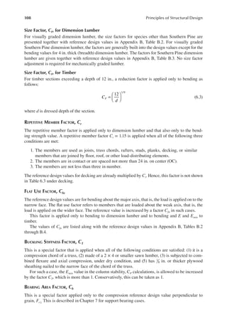
123. 105
6 Wood Speciications
ENGINEERING PROPERTIES OF SAWN LUMBER
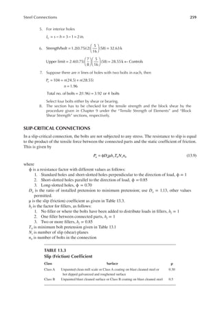
The National Design Speciication for Wood Construction of the American Forest and Paper
Association (2012 edition) provides the basic standards and speciications for sawn lumber and
engineered wood (e.g., glued laminated timber [GLULAM]) in the United States. The second part
of the National Design Speciication (NDS), referred to as the NDS supplement, contains numeri-
cal values for the strength of different varieties of wood grouped according to the species of trees.
Pieces of wood sawn from the same species or even the same source show a great variation in engi-
neering properties. Accordingly, the lumber is graded to establish strength values. Pieces of lumber
having similar mechanical properties are placed in the same class known as the grade of wood.
Most lumber is visually graded. However, a small percentage is mechanically graded. In each grade,
the relative size of wood section and the suitability of that size for a structural application are used
as additional guides to establish the strength.
A lumber is referred to by its nominal size. However, the lumber used in construction is mostly
dressed lumber. In other words, the lumber is surfaced to a net size, which is taken to be 0.5 in. less
than the nominal size for sizes up to 6 in., 0.75 in. less for nominal sizes over 6 in. and below 16 in.,
and 1 in. less for sizes 16 in. and above. In the case of large sections, sometimes the lumber is rough
sawed. The rough-sawed dimensions are approximately 1/8 in. larger than the dressed size.
Sawed lumber is classiied according to size into (1) dimension lumber and (2) timber. Dimension
lumber has smaller sizes. It has a nominal thickness of 2–4 in. and a width* of 2–16 in. Thus, the
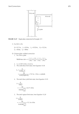
sizes of dimension lumber range from 2 in. × 2 in. to 4 in. × 16 in. Timber has a minimum nominal
thickness of 5 in.
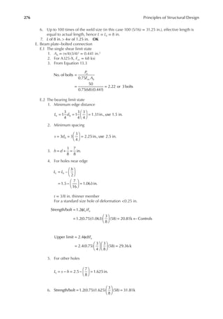
Dimension lumber and timber are further subdivided based on the suitability of the speciic
size for use as a structural member. The size and use categorization of commercial lumber is given
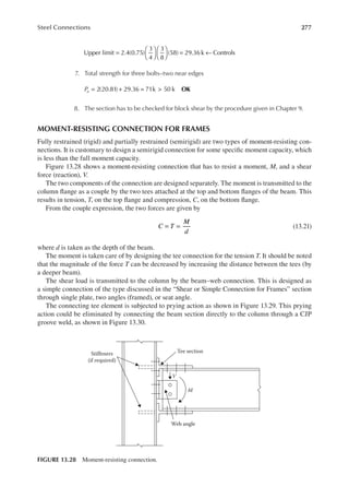
in Table 6.1. The sectional properties of standard dressed sawn lumber are given in Appendix B,
Table B.1.
REFERENCE DESIGN VALUES FOR SAWN LUMBER
The numerical values of permissible levels of stresses for design with respect to bending, tension,
compression, shear, modulus of elasticity, and modulus of stability of a speciic lumber are known
as reference design values. These values are arranged according to the species. Under each species,
size and use categories, as listed in Table 6.1, are arranged. For each size and use category, the ref-
erence design values are listed for different grades of lumber. Thus, design value may be different
for the same grade name but in a different size category. For example, the select structural grade
appears in SLP, SJ & P, beam and stringer (B & S), and post and timber (P & T) categories and the
design values for a given species are different for the select structural grade in all of these categories.
The following reference design values are provided in tables:
Appendix B, Table B.2: Reference design values for dimension lumber other than Southern
Pine
* In the terminology of lumber grading, the smaller cross-sectional dimension is thickness and the larger dimension is
width. In the designation of engineering design, the dimension parallel to the neutral axis of a section as placed is width
and the dimension perpendicular to the neutral axis is depth. Thus, a member loaded about the strong axis (placed with
the smaller dimension parallel to the neutral axis) has the width that is referred to as thickness in lumber terminology.

124. 106 Principles of Structural Design
Appendix B, Table B.3: Reference design values for Southern Pine dimension lumber
Appendix B, Table B.4: Reference design values for timber
Although reference design values are given according to the size and use combination, the values
depend on the size of the member rather than its use. Thus, a section 6 × 8 listed under the P & T
category with its reference design values indicated therein can be used for B & S, but its design
values as indicated for P & T will apply.
ADJUSTMENTS TO THE REFERENCE DESIGN VALUES FOR SAWN LUMBER
The reference design values in the NDS tables are the basic values that are multiplied by many
factors to obtain adjusted design values. To distinguish an adjusted value from a reference value, a
prime notation is added to the symbol of the reference value to indicate that necessary adjustments
have been made. Thus,
F F (products of adjustment factors)
( ) ( )
′ = × (6.1)
The () is replaced by a property like tensile, compression, and bending.
For wood structures, allowable stress design (ASD) is a traditional basis of design. The load
resistance factor design (LRFD) provisions were introduced in 2005. The reference design values
given in NDS are based on ASD (i.e., these are permissible stresses). The reference design values
for LRFD have to be converted from the ASD values.
To determine the nominal design stresses for LRFD, the reference design values of the NDS tables,
as reproduced in the appendixes, are required to be multiplied by a format conversion factor, KF.
The format conversion factor serves a purpose that is reverse of the factor of safety, to obtain the
nominal strength values for LRFD application. In addition, the format conversion factor includes
the effect of load duration. It adjusts the reference design values of normal (10 years) duration to the
nominal strength values for a short duration (10minutes), which have better reliability.
In addition to the format conversion factor, a resistance factor, ϕ, is applied to obtain the LRFD
adjusted values. A subscript n is added to recognize that it is a nominal (strength) value for the
LRFD design. Thus, the adjusted nominal design stress is expressed as follows:
( ) ( )
F F K
n F
′ = φ ′ (6.2)
TABLE 6.1
Categories of Lumber and Timber
Name Symbol
Nominal Dimension
Thickness (Smaller Dimension) Width
A. Dimension Lumber
1. Light framing LF 2–4 in. 2–4 in.
2. Structural light framing SLF 2–4 in. 2–4 in.
3. Structural joist and plank SJ & P 2–4 in. 5 in. or more
4. Stud 2–4 in. 2 in. or more
5. Decking 2–4 in. 4 in. or more
B. Timber
1. Beam and stringer B & S 5 in. or more At least 2 in. more than thickness
2. Post and timber P & T 5 in. or more Not more than 2 in. more than thickness

125. 107
Wood Speciications
The adjustment factors are discussed as follows:
1. The wet-service factor is applied when the wood in a structure is not in a dry condition,
that is, its moisture content exceeds 19% (16% in the case of laminated lumber). Most
structures use dry lumber for which CM = 1.
2. The temperature factor is used if a prolonged exposure to higher than normal temperature
is experienced by a structure. The normal condition covers the ordinary winter to summer
temperature variations and the occasional heating up to 150°F. For normal conditions, Ct = 1.
3. Some species of wood do not accept a pressure treatment easily and require incisions to
make the treatment effective. For dimension lumber only, a factor of 0.8 is applied to bend-
ing, tension, shear, and compression parallel to grains and a factor of 0.95 is applied to
modulus of elasticity and modulus of elasticity for stability.
4. In addition, there are some special factors like column stability factor, CP, and beam stabil-
ity factor, CL, that are discussed in the context of column and beam designs in Chapter 7.
The other adjustment factors that are frequently applied are discussed in the following sections.
TIME EFFECT FACTOR,* λ
Wood has the unique property that it can support a higher load when it is applied for a short duration.
The nominal reference design values are representative of a short-duration loading. For a loading of
long duration, the reference design values have to be reduced by a time effect factor. Different types
of loads represent different load durations. Accordingly, the time effect factor depends on combina-
tions of loads. For various load combinations, the time effect factor is given in Table 6.2. It should
be remembered that the factor is applied to the nominal reference (stress) value and not to the load.
SIZE FACTOR, CF
The size of a wood section has an effect on its strength. The factor for size is handled differently for
dimension lumber and for timber.
* The time effect factor is relevant only to load resistance factor design. For allowable stress design, this factor, known as
the load duration factor, CD, has different values.
TABLE 6.2
Time Effect Factor
Load Combination λ
1.4D 0.6
1.2D + 1.6L + 0.5(Lr or S) 0.7 when L is from storage
0.8 when L is from occupancy
1.25 when L is from impact
1.2D + 1.6(Lr or S) + (fL or 0.5W) 0.8
1.2D + 1.0W + fL + 0.5(Lr or S) 1.0
1.2D + 1.0E + fL + 0.2S 1.0
0.9D + 1.0W 1.0
0.9D + 1.0E 1.0
Note: f = 0.5 for L ≤ 100 psf; otherwise f = 1.

126. 108 Principles of Structural Design
Size Factor, cF, for Dimension Lumber
For visually graded dimension lumber, the size factors for species other than Southern Pine are
presented together with reference design values in Appendix B, Table B.2. For visually graded
Southern Pine dimension lumber, the factors are generally built into the design values except for the
bending values for 4 in. thick (breadth) dimension lumber. The factors for Southern Pine dimension
lumber are given together with reference design values in Appendix B, Table B.3. No size factor
adjustment is required for mechanically graded lumber.
Size Factor, cF, for Timber
For timber sections exceeding a depth of 12 in., a reduction factor is applied only to bending as
follows:
=






12
1/9
C
d
F (6.3)
where d is dressed depth of the section.
REPETITIVE MEMBER FACTOR, Cr
The repetitive member factor is applied only to dimension lumber and that also only to the bend-
ing strength value. A repetitive member factor Cr = 1.15 is applied when all of the following three
conditions are met:
1. The members are used as joists, truss chords, rafters, studs, planks, decking, or similar
members that are joined by loor, roof, or other load-distributing elements.
2. The members are in contact or are spaced not more than 24 in. on center (OC).
3. The members are not less than three in number.
The reference design values for decking are already multiplied by Cr. Hence, this factor is not shown
in Table 6.3 under decking.
FLAT USE FACTOR, Cfu
The reference design values are for bending about the major axis, that is, the load is applied on to the
narrow face. The lat use factor refers to members that are loaded about the weak axis, that is, the
load is applied on the wider face. The reference value is increased by a factor Cfu in such cases.
This factor is applied only to bending to dimension lumber and to bending and E and Emin to
timber.
The values of Cfu are listed along with the reference design values in Appendix B, Tables B.2
through B.4.
BUCKLING STIFFNESS FACTOR, CT
This is a special factor that is applied when all of the following conditions are satisied: (1) it is a
compression chord of a truss, (2) made of a 2 × 4 or smaller sawn lumber, (3) is subjected to com-
bined lexure and axial compression, under dry condition, and (5) has 3
8 in. or thicker plywood
sheathing nailed to the narrow face of the chord of the truss.
For such a case, the Emin value in the column stability, CP calculations, is allowed to be increased
by the factor CT, which is more than 1. Conservatively, this can be taken as 1.
BEARING AREA FACTOR, Cb
This is a special factor applied only to the compression reference design value perpendicular to
grain, Fc⊥ This is described in Chapter 7 for support bearing cases.

127. 109
Wood Speciications
FORMAT CONVERSION FACTOR, KF
The format conversion factors for different types of stresses are reproduced in Table 6.3 from
Table N1 of the NDS.
RESISTANCE FACTOR, ϕ
The resistance factor, also referred to as the strength reduction factor, is used to account for all
uncertainties whether related to the materials manufacturing, structural construction, or design
computations that may cause actual values to be less than theoretical values. The resistance factor,
given in Table 6.4, is a function of the mode of failure. The applicable factors for different loadings
and types of lumber are summarized in Table 6.5.
LOAD RESISTANCE FACTOR DESIGN WITH WOOD
As discussed in the “Working Stress, Strength Design, and Uniied Design of Structures” sec-
tion in Chapter 1, LRFD designs are performed at the strength level in terms of force and moment.
Accordingly, the adjusted nominal design stress values from the “Reference Design Values for Sawn
Lumber” section are changed to strength values by multiplying them by the cross-sectional area or
the section modulus. Thus, the basis of design in LRFD is as follows:
Bending: ( )
M M F S F C C C C C C C K S
u n bn b M t F r fu i L F
= φ = ′ = φ λ (6.4)
Tension: T T F C C C C K A
u n t M t F i F
= φ = φ λ (6.5)
TABLE 6.4
Resistance Factor, ϕ
Application Property ϕ
Member Fb 0.85
Ft 0.80
Fv, Frt 0.75
Fc, Fc⊥ 0.9
Emin 1.76
All connections All design values 0.65
TABLE 6.3
Conversion Factor for Stresses
Application Property KF
Member Bending Fb 2.54
Tension Ft 2.7
Shear Fv, radial tension Frt 2.88
Compression Fc 2.4
Compression perpendicular to grain Fc⊥ 1.67
Emin 1.76
E 1.0
All connections All design values 3.32

128. 110
Principles
of
Structural
Design
TABLE 6.5
Applicability of Adjustment Factors for Sawn Lumber
Loading Condition Type of Lumber
Factor Special Factor
Time
Effect
Size
Effect Repetitive
Wet
Service Temperature Incision
Flat
Use
Beam
Stability
Column
Stability
Buckling
Stiffness
Bearing
Area
Bending Dimension lumber:
visually graded
λ CF Cr CM Ct Ci Cfu CL
Dimension lumber:
mechanically graded
λ Cr CM Ct Ci Cfu CL
Timber λ CF CM Ct Cfu CL
Decking λ CF CM Ct CL
Tension Dimension lumber λ CF CM Ct Ci
Compression—parallel to
grain
Dimension lumber λ CF CM Ct Ci CP
Timber λ CM Ct CP
Compression—normal to
grain
Both λ CM Ct Ci Cb
Shear parallel to grain Both λ CM Ct Ci
Modulus of elasticity Both CM Ct Ci
a
Modulus of elasticity for
stability
Both CM Ct Ci
a CT
a Only for timber of structural #1, a Cfu of 0.9 is applied to E and Emin (in addition to table values for Fb). For all other species of timber, Cfu is 1 for E and Emin.

129. 111
Wood Speciications
Compression: ( )
P P F C C C C C K A
u n C M t F i P F
= φ = φ λ (6.6)
P P F C C C C K A
u n c M t i b F
= φ = φ λ
⊥ ⊥ (6.7)
V V F C C C K A
u n v M t i F
= φ = φ λ






Shear:
2
3
* (6.8)
E E C C C C K
min(n) min M t i T F
φ
=
Stability: (6.9)
E EC C C
n M t i
=
Modulus of elasticity: ( ) (6.10)
The left-hand side (LHS) in the aforementioned equations represent the factored design loads com-
bination and the factored design moments combination.*
The design of an element is an iterative procedure since the reference design values and the modii-
cation factors in many cases are a function of the size of the element that is to be determined. Initially,
the nominal design value could be assumed to be one-and-a-half times the basic reference design value
for the smallest listed size of the speciied species from the Tables B.2 through B.4 in Appendix B.
Example 6.1
Determine the adjusted nominal reference design values and the nominal strength capacities of the
Douglas Fir-Larch #1 2 in. × 8 in. roof rafters at 18 in. on center (OC) that support dead and roof
live loads. Consider dry-service conditions, normal temperature range, and no-incision application.
SOLUTION
1. The reference design values of a Douglas Fir-Larch #1 2 in. × 8 in. section are obtained from
Appendix B, Table B.2.
2. The adjustment factors and the adjusted nominal reference design values are computed in
the following table:
3. Strength capacities
For a 2 in. × 8 in. section, S = 13.14 in.3 and A = 10.88 in.2
Mu = F′
bnS = (2383.54)(13.14) = 31319.66 in.·lb
Tu = F′
tnA = (1399.68)(10.88) = 15228.52 lb
Vu = F′vn(2A/3) = (311.04)(2 × 10.88/3) = 2257.21 lb
Pu = F′
cnA = (2721.6)(10.88) = 29611 lb
*
τ = = τ 





3
2
or
2
3
max max
V
A
V A
Property Reference Design Value (psi)
Adjustment Factors
F′
()n (psi)
ϕ λ for D + Lr cF cr KF
Bending 1000 0.85 0.8 1.2 1.15 2.54 2383.54
Tension 675 0.80 0.8 1.2 2.7 1399.68
Shear 180 0.75 0.8 2.88 311.04
Compression 1500 0.9 0.8 1.05 2.40 2721.6
Compression ⊥ 625 0.9 0.8 1.67 751.5
E 1.7 × 106 1.7 × 106
Emin 0.62 × 106 0.85 1.76 0.93 × 106

130. 112 Principles of Structural Design
Example 6.2
Determine the adjusted nominal reference design values and the nominal strength capacities of a
Douglas Fir-Larch #1 6 in. × 16 in. loor beam supporting a combination of loads comprising dead,
live, and snow loads. Consider dry-service conditions, normal temperature range, and no-incision
application.
SOLUTION
1. The reference design values of Douglas Fir-Larch #1 6 in. × 16 in. beams and stringers are
from Appendix B, Table B.4.
2. The adjustment factors and the adjusted nominal reference design values are given in the
following table:
3. Strength capacities
For the 6 in. × 16 in. section, S = 206.3 in.3 and A = 82.5 in.2
Mu = F′bnS = (2275.76)(206.3) = 469,489 in.·lb
Tu = F′
tnA = (1166.4)(82.5) = 96,228 lb
Vu = F′
vn(2A/3) = (293.8)(2 × 82.5/3) = 16,167 lb
Pu = F′
cnA = (1598.4)(82.5) = 131,868 lb
Example 6.3
Determine the unit load (per square foot load) that can be imposed on a loor system consisting of
2 in. × 6 in. Southern Pine select structural joists spaced at 24 in. OC spanning 12 ft. Assume that
the dead load is one-half of the live load. Ignore the beam stability factor.
SOLUTION
1. For Southern Pine 2 in. × 6 in. select structural dressed lumber, the reference design value is
2550psi
=
Fb .
2. Size factor is included in the tabular value.
3. Time effect factor for dead and live loads = 0.8
4. Repetitive factor = 1.15
5. Format conversion factor = 2.54
6. Resistance factor = 0.85
7. Nominal reference design value
0.85(2250)(0.8)(1)(1)(1)(1.15)(1)(1)(2.54) 5065 psi
′ = φ λ
= =
F F C C C C C C K
bn b M t i r F fu F
Property Reference Design Value (psi)
Adjustment Factors
F′
()n (psi)
ϕ λ for D, L, S cF
a KF
Bending 1350 0.85 0.8 0.976 2.54 2275.76
Tension 675 0.80 0.8 2.70 1166.4
Shear 170 0.75 0.8 2.88 293.8
Compression 925 0.9 0.8 2.4 1598.4
E 1.6 × 106 1.6 × 106
Emin 0.58 × 106 0.85 1.76 0.87 × 106
a
C
d
F = 




 = 




 =
12 12
15
0.976.
1/9 1/9

131. 113
Wood Speciications
8. For 2 in. × 6 in., S = 7.56 in.3
9. Mu = F′bnS = (5065)(7.56) = 38291.4 in.·lb or 3191 ft.·lb
10.
8
2
=
M
w L
u
u
or
8 8 3191
12
177.3 lb/ft.
2
( )
( )
= = =
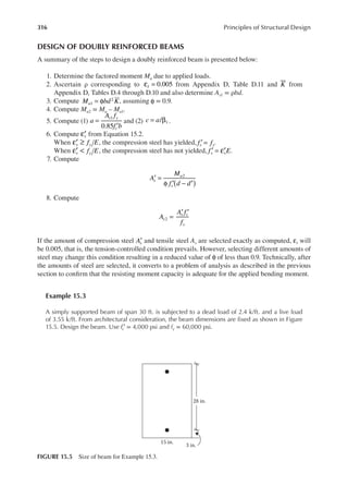
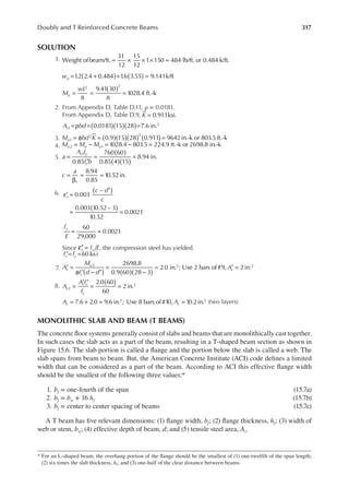
2
w
M
L
u
u
11. Tributary area per foot of joists = 24
12
1 2ft. /ft.
2
× =
12. wu = (Design load per square foot) (Tributary area per square foot)
( )
= +
177.3 (1
.2 1
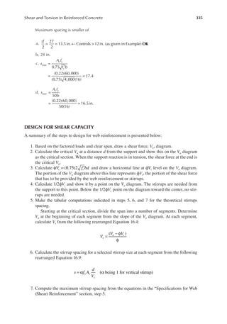
.6 ) 2
D L
or
D
177.3 1
.2 1
.6 2 2
D
[ ]
( ) ( )
= +
or
20.15lb/ft.2
D =
and
40.3lb/ft.2
L =
Example 6.4
For a Southern Pine #1 loor system, determine the size of joists at 18 in. OC spanning 12 ft. and
the column receiving loads from an area of 100 ft.2 acted upon by a dead load of 30 psf and a live
load of 40 psf. Assume that the beam and column stability factors are not a concern.
SOLUTION
A. Joist design
1. Factored unit combined load = 1.2(30) + 1.6(40) = 100 psf
2. Tributary area/ft. = (18/12) × 1 = 1.5 ft.2/ft.
3. Design load/ft. wu = 100(1.5) = 150 lb/ft.
4.
8
(150)(12)
8
2,700ft. lbor32,400in. lb
2 2
= = = ⋅ ⋅
M
w L
u
u
5. For a trial section, select the reference design value of a 2–4 in. wide section and
assume the nominal reference design value to be one-and-a-half times the table value.
From Appendix B, Table B.3, for Southern Pine #1, Fb = 1850 psi
Nominal reference design value = 1.5(1850) = 2775 psi
6. Trial size
32,400
2,775
11.68in.3
=
′
= =
S
M
F
u
bn
Use 2 in. × 8 in. S = 13.14 in.3
7. From Appendix B, Table B.3, Fb = 1500 psi
8. Adjustment factors
0.8
λ =
1.15
=
Cr
2.54
=
KF
0.85
φ =
9. Adjusted nominal reference design value
0.85 1500 0.8 1
.15 2.54 2979.4 psi
( )( )( )( )
′ = =
Fbn
10. = ′
M F S
u bn
or
S
M
F
reqd
u
bn
32,400
2,979.4
10.87 13.14 in.3
=
′
= = ≤
The selected size 2 in. × 8 in. is OK.

132. 114 Principles of Structural Design
B. Column design
1. Factored unit load (step A.1) = 100 psf
2. Design load = (unit load)(tributaryarea)
(100)(100) 10,000 lb
= =
3. For a trial section, select the reference design value of a 2–4 in. wide section and
assume the nominal reference design value to be one-and-a-half times of the table
value.
From Appendix B, Table B.3, for Southern Pine #1, Fc = 1850 psi
Nominal reference design value = 1.5(1850) = 2775 psi
4. Trial size
10,000
2,775
3.6 in.2
=
′
= =
A
P
F
u
cn
Use 2 in. × 4 in. A = 5.25 in.2
5. 1850 psi
0.8
2.40
0.90
=
λ =
=
φ =
F
K
b
F
6. Adjusted nominal reference design value
F
A
P
F
cn
reqd
u
cn
0.9 1,850 0.8 2.4 3,196.8 psi
10,000
3,196.8
3.13 5.25 in.2
) ) )
( ( (
′ = =
=
′
= = <
The selected size 2 in. × 4 in. is OK.
STRUCTURAL GLUED LAMINATED TIMBER
GLULAM members are composed of individual pieces of dimension lumber that are bonded together
by an adhesive to create required sizes. For western species, the common widths* (breadth) are 3 ,
1
8 5
1
8, 63
4, 83
4, 103
4, and 121
2 in. (there are other interim sections as well). The laminations are typically
in 11
2 in. incremental depth. For Southern Pine, the common widths are 3, 5, 63
4, 81
2, and 101
2 in. and
the depth of each lamination is 13
8 in. Usually, the lamination of GLULAM is horizontal (the wide
faces are horizontally oriented). A typical cross section is shown in Figure 6.1.
* Not in terms of lumber grading terminology.
Width 3, 5,…10½ Southern Pine
1½ in. Western species
1⅜ in. Southern Pine
Width 3⅛, 5⅛,…10¾ Western species
Side
Edge of lamination
Wide face of
lamination
Lamination
thickness
End
FIGURE 6.1 A structural glued laminated (GLULAM) section.

133. 115
Wood Speciications
The sectional properties of western species structural GLULAM are given in Appendix B,
Table B.5 and those of Southern Pine structural GLULAM in Appendix B, Table B.6.
Because of their composition, large GLULAM members can be manufactured from smaller trees
from a variety of species such as Douglas Fir, Hem Fir, and Southern Pine. GLULAM has much
greater strength and stiffness than sawn lumber.
REFERENCE DESIGN VALUES FOR GLUED LAMINATED TIMBER
The reference design values for GLULAM are given in Appendix B, Table B.7 for members stressed
primarily in bending (beams) and in Appendix B, Table B.8 for members stressed primarily in axial
tension or compression.
Appendix B, Table B.7 related to bending members is a summary table based on the stress
class. The irst part of the stress class symbol refers to the bending stress value for the grade in
hundreds of pounds per square inch followed by the letter F. For example, 24F indicates a bending
stress of 2400 psi for normal duration loaded in the normal manner, that is, loads are applied
perpendicular to the wide face of lamination. The second part of the symbol is the modulus of
elasticity in millions of pounds per square inch. Thus, 24F-1.8E indicates a class with the bending
stress in 2400 psi and the modulus of elasticity in 1.8 × 106 psi. For each class, the NDS provide
the expanded tables that are orgainzed according to the combination symbol and the types of
species making up the GLULAM. The irst part of the combination symbol is the bending stress
level, that is, 24F referring to 2400 psi bending stress. The second part of the symbol refers to the
lamination stock: V standing for visually graded and E for mechanically graded or E-rated. Thus,
the combination symbol 24F-V5 refers to the grade of 2400 psi bending stress of visually graded
lumber stock. Under this, species are indicated by abbreviations, that is, DF for Douglas Fir, SP for
Southern Pine, and HF for Hem Fir.
The values listed in Appendix B, Table B.7 are more complex than those for sawn lumber. The
irst six columns are the values for bending about the strong (x–x) axis when the loads are per-
pendicular to the wide face of lamination. These are followed up values for bending about the
y–y axis. The axially loaded values are also listed in case the member is picked up for the axial load
conditions.
For Fbx, two values have been listed in columns 1 and 2 of Appendix B, Table B.7 (for
bending) as Fbx
+ and Fbx
−. In a rectangular section, the compression and tension stresses are
equal in extreme ibers. However, it has been noticed that the outer tension laminations are in a
critical state and, therefore, high-grade laminations are placed at the bottom of the beam, which
is recognized as the tensile zone of the beam. The other side is marked as the top of the beam in
the lamination plant. Placed in this manner, the portion marked top is subjected to compression
and the bottom to tension. This is considered as the condition in which the designated tension
zone is stressed in tension and the Fbx
+ value of the irst column is used for bending stress. This
is a common condition.
However, if the beam is installed upside down or in the case of a continuous beam for which the
negative bending moment condition develops, that is, the top ibers are subject to tension, the refer-
ence values in the second column known as the designated compression zone stressed in tension,
Fbx
−, should be used.
Appendix B, Table B.8 lists the reference design values for principally axially load-carrying
members. Here, members are identiied by numbers, such as 1, 2, and 3, followed by species such
as DF, HF, and SP, and by grade. The values are not complex like those in Appendix B, Table B.7
(the bending case).
It is expected that members with the bending combination in Appendix B, Table B.7 will be
used as beams, as they make eficient beams. However, it does not mean that they cannot be used

134. 116 Principles of Structural Design
for axial loading. Similarly, an axial combination member can be used for a beam. The values with
respect to all types of loading modes are covered in both tables (Appendix B, Tables B.7 and B.8).
ADJUSTMENT FACTORS FOR GLUED LAMINATED TIMBER
The reference design values of Appendix B, Tables B.7 and B.8 are applied by the same format
conversion factors and time effect factors as discussed in the “Adjustments to the Reference Design
Values for Sawn Lumber” section.
Additionally, the other adjustment factors listed in Table 6.6 are applied to structural GLULAM.
For GLULAM, when moisture content is more than 16% (as against 19% for sawn lumber), the
wet-service factor is speciied in a table in the NDS. The values are different for sawn lumber and
GLULAM. The temperature factor is the same for GLULAM as for sawn lumber.
The beam stability factor, CL, column stability factor, CP, and bearing area factor, Cb, are the same
as for the sawn lumber. However, some other factors that are typical to GLULAM are described in
the following sections.
FLAT USE FACTOR FOR GLUED LAMINATED TIMBER, Cfu
The lat use factor is applied to the reference design value only (1) for the case of bending that is
loaded parallel to laminations and (2) if the dimension parallel to the wide face of lamination (depth
in lat position) is less than 12 in. The factor is
C
d
fu =






12
1/9
(6.11)
where d is depth of the section.
Equation 6.11 is similar to the size factor (Equation 6.3) of sawn timber lumber.
VOLUME FACTOR FOR GLUED LAMINATED TIMBER, CV
The volume factor is applied to bending only for horizontally laminated timber for loading applied
perpendicular to laminations (bending about the x–x axis); it is applied to Fbx
+ and Fbx
–. The beam
stability factor, CL, and the volume factor, Cv, are not used together; only the smaller of the two is
applied to adjust Fbn
′ . The concept of the volume factor for GLULAM is similar to the size factor for
sawn lumber because test data have indicated that the size effect extends to volume in the case of
GLULAM. The volume factor is
=

















 ≤
5.125 12 21
1
1/ 1/ 1/
C
b d L
v
x x x
(6.12)
where
b is width (in inches)
d is depth (in inches)
L is length of member between points of zero moments (in feet)
x = 20 for Southern Pine and 10 for other species
CURVATURE FACTOR FOR GLUED LAMINATED TIMBER, CC
The curvature factor is applied to bending stress only to account for the stresses that are introduced
in laminations when they are bent into curved shapes during manufacturing. The curvature factor is
= − 





1 2000
2
C
t
R
c (6.13)

135. 117
Wood
Speciications
TABLE 6.6
Applicability of Adjustment Factors for GLULAM
Loading Condition Loading Case Factor Special Factor
Time
Effect
Wet
Service Temperature
Size
(Volume)
Flat
Use Curvature
Beam
Stability
Column
Stability
Stress
Interaction
Shear
Reduction
Bearing
Area
Bending Load perpendicular
to lamination
λ CM Ct Cv Cc CL (or Cv) CI
Load parallel to
lamination
λ CM Ct Cfu Cc CL CI
Tension λ CM Ct
Compression Load parallel to
grain
λ CM Ct CP
Load perpendicular
to grain
λ CM Ct Cb
Shear λ CM Ct Cvr
Modulus of elasticity CM Ct
Modulus of elasticity
for stability
CM Ct

136. 118 Principles of Structural Design
where
t is thickness of the lamination, 11
2 in. or 13
8 in.
R is radius of curvature of the inside face of the lamination
The ratio t/R may not exceed 1/100 for Southern Pine and 1/125 for other species. The curvature
factor is not applied to the straight portion of a member regardless of curvature in the other portion.
STRESS INTERACTION FACTOR, CI
This is applied only (1) to the tapered section of a member and (2) to the reference bending stress.
For members tapered in compression, either CI or the volume factor Cv is applied, whichever is
smaller. For members tapered on tension face, either CI or the beam stability factor CL is applied,
whichever is smaller.
The factor depends on the angle of taper, bending stress, shear stress, and compression stress
perpendicular to grains for compression face taper and radial tensile stress for tensile face taper. It
is less than 1. A reference is made to Section 5.3.9 of NDS 2012.
SHEAR REDUCTION FACTOR, CVR
The reference shear design values Fvx and Fvy are multiplied by a factor Cvr = 0.72 when any of the
following conditions apply:
1. Nonprismatic members
2. Members subject to impact or repetitive cyclic loading
3. Design of members at notches
4. Design of members at connections
Example 6.5
Determine the adjusted nominal reference design stresses and the strength capacities of a 63
⁄4
in. × 18 in. GLULAM from Douglas Fir-Larch of stress class 24F-1.7E, used primarily for bend-
ing. The span is 30 ft. The loading consists of the dead load and live load combination along
the major axis.
SOLUTION
1. The adjusted reference design values are computed in the following table:
Property Reference Design Value (psi) Adjustment Factors F()n
ʹ (psi)
ϕ λ cv KF
Bending 2400 0.85 0.8 0.90a 2.54 3730.75
Tension 775 0.8 0.8 2.7 1339.2
Shear 210 0.75 0.8 2.88 362.88
Compression 1000 0.9 0.8 2.4 1728.0
E 1.7 × 106 1.7 × 106
Emin 0.88 × 106 0.85 1.76 1.32 × 106
a
= 
















 =
5.125
6.75
12
18
21
30
0.90
1 10 1 10 1 10
Cv

137. 119
Wood Speciications
2. Strength capacities:
For the 63
4 in. × 18 in. section, Sx = 364.5 in.3, A = 121.5 in.2
Bending: ϕMn = ′
F S
bn = (3730.75)(364.5) = 1.36 × 106 in.·lb
Tension: ϕTn = ′
F A
tn = (1339.2)(121.5) = 162.71 × 103 lb
Shear: ϕVn = (2/3 )
′
F A
vn = (362.88)(2/3 × 121.5) = 29.39 × 103 lb
Compression: ϕPn = ′
F A
cn = (1728)(121.5) = 210 × 103 lb
Example 6.6
The beam in Example 6.5 is installed upside down. Determine the design strengths.
SOLUTION
1. The bending reference design value for a compression zone stressed in tension = 1450 psi
from Appendix B, Table B.7
2. Adjustment factors from Example 6.5
Φ = 0.85
0.80
λ =
0.90
=
Cv
2.54
=
KF
3. Adjusted nominal design value
0.85 1450 0.8 0.9 2.54 2254 psi
( )( )( )( )
′ = =
Fbn
4. Strength capacity
2254 364.5 0.882 10 in.lb
6
( )( )
′ = = × ⋅
F S
bn
5. The other values are the same as in Example 6.5.
Example 6.7
The beam used in Example 6.5 is lat with loading along the minor axis. Determine the design
strengths.
SOLUTION
1. The adjusted reference design values are computed in the following table:
Property Reference Design Value (psi) Adjustment Factors F()n
′ (psi)
ϕ λ cfu KF
Bending 1050 0.85 0.8 1.066a 2.54 1933.26
Tension 775 0.8 0.8 2.7 1339.2
Shear 185 0.75 0.8 2.88 319.68
Compression 1000 0.9 0.8 2.4 1728.0
E 1.3 × 106 1.3 × 106
Emin 0.67 × 106 0.85 1.76 1.00 × 106
a
= 




 =
12
6.75
1.066
1 9
Cfu

138. 120 Principles of Structural Design
2. Strength capacities
For the 6¾ in. × 18 in. section, Sy = 136.7 in.3, A = 121.5 in.2
Bending: ϕMn = ′
F S
bn = (1933.26)(136.7*) = 0.26 × 106 in.·lb
Tension: ϕTn = ′
F A
tn = (1339.2)(121.5) = 162713 lb
Shear: ϕVn = (2/3 )
′
F A
vn = (319.68)(2/3 × 121.5) = 25.89 × 103 lb
Compression: ϕPn = ′
F A
cn = (1728)(121.5) = 209 × 103 lb
Example 6.8
What are the unit dead and live loads (per square foot) resisted by the beam in Example 6.5 that
is spaced 10 ft. OC? Assume that the unit dead load is one-half of the live load.
SOLUTION
1. From Example 6.5,
1.36 10 . Ib or 113,333.3 ft. Ib
6
= φ = × ⋅ ⋅
M M
u n
2. 113,333.33
8
2
= =
M
w L
u
u
or
113,333.33(8)
(30)
1,007.41lb/ft.
2
= =
wu
3. Tributary area per foot of the beam = 10 × 1 = 10 ft.2/ft.
(Designload/ft. )(Tributary area, ft. /ft.)
2 2
=
wu
D L
1007.41 (1.2 1.6 )(10)
= +
or
D D
1007.41 [1.2 1.6(2 )](10)
= +
or
D 22.9lb/ft.2
=
and
L 45.8lb/ft.2
=
STRUCTURAL COMPOSITE LUMBER
Structural composite lumber (SCL) is an engineered product manufactured from smaller logs. The
manufacturing process involves sorting and aligning strands or veneer, applying adhesive, and
bonding under heat and pressure. Stranding is making 3–12 in. slices of a log similar to grating a
block of cheese. Veneering is rotary peeling by a knife placed parallel to the outer edge of a spin-
ning log. The log is peeled from outside toward the center similar to removing paper towels from a
roll. The slices cut into sheets are called veneer.
The following are four common types of SCL products:
1. Laminated strand lumber
2. Oriented strand lumber
3. Laminated veneer lumber (LVL)
4. Parallel strand lumber
* Sy value.

139. 121
Wood Speciications
The irst two of these are strand products and the last two are veneer products. Proprietary names,
such as Microlam and Parallam, are used to identify the aforementioned products.
The lamination of SCL is vertical (wide faces of laminations are oriented vertically) compared
to the horizontal lamination of GLULAM (wide faces are oriented horizontally). The strength and
stiffness of SCL is generally higher than that of GLULAM.
The typical reference design values for SCL are listed in Appendix B, Table B.9. SCL is equally
strong latwise and edgewise in bending. Several brands of SCL are available. The reference
values and technical speciications for a speciic brand might be obtained from the manufacturer’s
literature.
The same time effect factors and format conversion factors are applied to the reference design
values of SCL as for sawn lumber and GLULAM, as discussed in the “Adjustments to the Reference
Design Values Sawn Lumber” section.
In addition, the adjustment factors listed in Table 6.7 are applied to SCL. The wet-service factors,
CM, and the temperature factors, Ct, are the same for GLULAM and SCL. To the members used
in repetitive assembly, as deined in the “Repetitive Member Factor, Cr” section of sawn lumber, a
repetitive factor, Cr, of 1.04 is applied.
The value of the size (volume) factor, Cv, is obtained from the SCL manufacturer’s litera-
ture. When Cv ≤ 1, only the lesser of the volume factor, Cv, and the beam stability factor, CL,
is applied. However, when Cv > 1 both the volume factor and the beam stability factor are used
together.*
SUMMARY OF ADJUSTMENT FACTORS
A. Common to sawn lumber, GLULAM, and SCL
1. Time effect, λ ≤ 1
2. Temperature, Ct ≤ 1
3. Wet service, CM ≤ 1
4. Format conversion, KF > 1
5. Resistance factor, ϕ < 1
6. Beam stability factor, CL (applied to Fb only) ≤ 1
7. Column stability factor, CP (applied only to Fc parallel to grain) ≤ 1
8. Bearing area factor, Cb (applied only to Fc perpendicular to grain) ≥ 1
B. Sawn lumber
1. Incision factor, Ci ≤ 1
2. Size factor, CF ≤ 1
3. Repetitive factor, Cr = 1.15
4. Flat use factor, Cfu (applied only to Fb) for dimension ≥1, for timber ≤1
C. GLULAM
1. Volume factor, Cv ≤ 1
2. Curvature factor, Cc ≤ 1
3. Flat use factor, Cfu (applied only to Fb) for GLULAM ≥1
D. SCL
1. Volume factor, Cv ≤ 1 or Cv ≥ 1
2. Repetitive factor, Cr = 1.04
E. Special factors
1. Buckling stiffness factor, CT (applied only to sawn lumber and to Emin) ≥ 1
2. Stress interaction factor, CI (applied only to GLULAM and tapered section) ≤ 1
3. Shear reduction factor, Cvr (applied only to GLULAM and to Fv in some cases) = 0.72
* When the volume factor Cv > 1, it is used in the calculation of beam stability factor, as discussed in Chapter 7.

140. 122
Principles
of
Structural
Design
TABLE 6.7
Applicability of Adjustment Factors for SCL
Loading Condition Loading Case
Factor Special Factor
Time
Effect
Wet
Service Temperature
Size
(Volume) Repetitive
Beam
Stability
Column
Stability
Bearing
Area
Bending Load perpendicular to
lamination
λ CM Ct Cv
a Cr CL
a
Tension λ CM Ct
Compression Load parallel to grain λ CM Ct CF
Load perpendicular to grain λ CM Ct Cb
Shear λ CM Ct
Modulus of elasticity CM Ct
Modulus of elasticity
for stability
CM Ct
a For SCL, when Cv ≤ 1 the lesser of Cv and CL is applied. When Cv > 1, both Cv and CL are applied.

141. 123
Wood Speciications
PROBLEMS
Note: In Problems 6.1 through 6.5, determine the adjusted reference design values and the strength
capacities for the following members. In all cases, consider dry-service conditions, normal tem-
perature range, and no-incision application. In practice, all loading combinations must be checked.
However, in these problems only a single load condition should be considered for each member, as
indicated in the problem.
6.1 Floor joists are 2 in. × 6 in. at 18 in. on center (OC) of Douglas Fir-Larch #2. They support
dead and live loads.
6.2 Roof rafters are 2 in. × 8 in. at 24 in. OC of Southern Pine #2. The loads are dead load and
roof live load.
6.3 Five loor beams are of 4 in. × 8 in. dimension lumber Hem Fir #1, spaced 5 ft. apart. The
loads are dead and live loads.
6.4 Studs are 2 in. × 8 in. at 20 in. OC of Hem Fir #2. The loads are dead load, live load, and
wind load.
6.5 The interior column is 5 in. × 5 in. of Douglas Fir-Larch #2 to support the dead and live
loads.
6.6 Determine the unit dead and live loads (per square foot area) that can be resisted by a loor
system consisting of 2 in. × 4 in. joists at 18 in. OC of Douglas Fir-Larch #1. The span is
12 ft. The dead and live loads are equal.
6.7 Determine the unit dead load on the roof. The roof beams are 4 in. × 10 in. of Hem Fir #1.
The beams are located at 5 ft. OC, and the span is 20 ft. apart. They support the dead load
and a snow load of 20 psf.
6.8 A 6 in. × 6 in. column of Douglas Fir-Larch #1 supports the dead load and live load on an
area of 100 ft.2 Determine the per-square-foot load if the unit dead load is one-half of the
unit live load.
6.9 A loor system is acted upon by a dead load of 20 psf and a live load of 40 psf. Determine
the size of the loor joists of Douglas Fir-Larch Structural lumber. They are located 18 in.
OC and span 12 ft. Assume that beam stability factor is not a concern.
6.10 In Problem 6.9, determine the size of the loor joists when used in the lat position.
6.11 Determine the size of a column of Southern Pine #2 of dimension lumber that receives
loads from an area of 20 ft. × 25 ft. The unit service loads are 20 psf dead load and 30 psf
live load. Assume that the column stability factor is not a concern.
6.12 For Problem 6.11, design a column of Southern Pine #2 timber.
6.13 A GLULAM beam section is 63
4 in. × 37.5 in. from the Douglas Fir 24F-1.7E class. The
loads combination comprises the dead load, snow load, and wind load. The bending is
about the x axis. Determine the adjusted nominal reference design stresses and the strength
capacities for bending, tension, shear, compression, modulus of elasticity, and modulus of
stability (Emin). The span is 30 ft.
6.14 Determine the wind load for Problem 6.13 if the unit dead load is 50 psf and the unit snow
and wind loads are equal. The beams are 10 ft. apart.
6.15 The beam in Problem 6.13 is installed upside down. Determine the strength capacities.
6.16 The beam in Problem 6.13 is used lat with bending about the minor axis. Determine the
design capacities.
6.17 A 51
8 in. × 28.5 in. 26F-1.9E Southern Pine GLULAM is used to span 35 ft. The beam has
a radius of curvature of 10 ft. The load combination is the dead load and the snow load.
Determine the adjusted nominal reference design stresses and the strength capacities for
loading perpendicular to the laminations for the beam installed according to speciications.
6.18 The beam in Problem 6.17 is installed upside down. Determine the percentage reduction in
strength capacities.

142. 124 Principles of Structural Design
6.19 The beam in Problem 6.17 is loaded along the laminations, about the minor axis. Determine
the percentage change in strength capacities.
6.20 A 13
4 in. × 71
4 in. size LVL of 1.9E class is used for roof rafters spanning 20 ft., located 24
in. OC. Determine the strength design capacities for the dead and snow load combinations.
The size factor is given by (12/d)1/7.5.
6.21 Two 13
4 in. × 16 in. (two sections side by side) of Parallam of 2.0E class are used for a
loor beam spanning 32 ft., spaced 8 ft. OC. The loading consists of dead and live loads.
Determine the strength capacities for bending, tension, composition, and shear. The size
factor is given by (12/d)1/7.5.
6.22 Determine the unit loads (per square foot) on the beam in Problem 6.21 if the live load is
one-and-a-half times the dead load.

143. 125
7 Flexure and Axially Loaded
Wood Structures
INTRODUCTION
The conceptual design of wood members was presented in Chapter 6. The underlying assumption
of design in that chapter was that an axial member was subjected to axial tensile stress or axial
compression stress only and a lexure member to normal bending stress only. However, the com-
pression force acting on a member tends to buckle a member out of the plane of loading, as shown in
Figure 7.1. This buckling occurs in the columns and in the compression lange of the beams unless
the compression lange is adequately braced. The beam and column stability factors CL and CP,
respectively, mentioned in the “Reference Design Values for Sawn Lumber” section of Chapter 6,
are applied to account for the effect of this lateral buckling.
This chapter presents the detailed designs of lexure members, axially loaded tensile and com-
pression members, and the members subjected to the combined lexure and axial force made of
sawn lumber, glued laminated timber (GLULAM), and laminated veneer lumber (LVL).
DESIGN OF BEAMS
In most cases, for the design of a lexure member or beam, the bending capacity of the material is
a critical factor. Accordingly, the basic criterion for the design of a wood beam is developed from a
bending consideration.
In a member subjected to lexure, compression develops on one side of the section; under com-
pression, lateral stability is an important factor. It could induce a buckling effect that will under-
mine the moment capacity of the member. An adjustment factor is applied in wood design when the
buckling effect could prevail, as discussed subsequently.
A beam is initially designed for the bending capacity. It is checked for the shear capacity. It is
also checked from the serviceability consideration of the limiting state of delection. If the size is
not found adequate for the shear capacity or the delection limits, the design is revised.
The bearing strength of a wood member is considered at the beam supports or where loads from
other members frame onto the beam. The bearing length (width) is designed on this basis.
BENDING CRITERIA OF DESIGN
For the bending capacity of a member, as discussed before
M F S
u bn
= ′ (7.1)
Mu represents the design moment due to the factored combination of loads. The design moment
for a uniformly distributed load, wu, is given by 8
2
M w L
u u
= and for a concentrated load, Pu
centered at mid-span, 4
M P L
u u
= . For other cases, Mu is ascertained from the analysis of structure.
For standard loading cases, Mu is listed in Appendix A, Table A.3.
The span length, L, is taken as the distance from the center of one support to the center of the
other support. However, when the provided (furnished) width of a support is more than what is

144. 126 Principles of Structural Design
required from the bearing consideration, it is permitted to take the span length to be the clear dis-
tance between the supports plus one-half of the required bearing width at each end.
′
Fbn is the adjusted load resistance factor design (LRFD) reference value for bending. To start
with, the reference bending design value, Fb, for the appropriate species and grade is obtained.
These values are listed in Appendices B.2 through B.4 for sawn lumber and Appendices B.7 through
B.9 for GLULAM and LVL. Then the value is adjusted by multiplying the reference value by a
string of factors. The applicable adjustment factors were given in Table 6.5 for sawn lumber, in
Table 6.6 for GLULAM, and in Table 6.7 for structural composite lumber (SCL).
For sawn lumber, the adjusted reference bending design value is restated as
′ = φ λ
F F C C C C C C C K
bn b M t F r fu i L F (7.2)
For GLULAM, the adjusted reference bending design value is restated as
( )
′ = φ λ or
F F C C C C C C C K
bn b M t c fu I v L F (7.3)
For SCL, the adjusted reference bending design value is
( )
′ = φ λ or/and
F F C C C C C K
bn b M t r v L F (7.4)
where
Fb is tabular reference bending design value
ϕ is resistance factor for bending = 0.85
λ is time factor (Table 6.2)
CM is wet-service factor
Ct is temperature factor
CF is size factor
Cr is repetitive member factor
Cfu is lat use factor
Ci is incision factor
CL is beam stability factor
Cc is curvature factor
Cv is volume factor
CI is stress interaction factor
KF is format conversion factor = 2.54
Using the assessed value of ′
Fbn, from Equations 7.2 through 7.4, based on the adjustment factors
known initially, the required section modulus, S, is determined from Equation 7.1 and a trial section
is selected having the section modulus S higher than the computed value. In the beginning, some
FIGURE 7.1 Buckling due to compression.

145. 127
Flexure and Axially Loaded Wood Structures
section-dependent factors such as CF, Cv, and CL will not be known while the others such as λ, KF,
and ϕ will be known. The design is performed considering all possible load combinations along
with the relevant time factor. If loads are of one type only, that is, all vertical or all horizontal, the
highest value of the combined load divided by the relevant time factor determines which combina-
tion is critical for design.
Based on the trial section, all adjustment factors including CL are then computed and the magni-
tude of ′
Fbn is reassessed. A revised S is obtained from Equation 7.1 and the trial section is modiied,
if necessary.
BEAM STABILITY FACTOR, cL
As stated earlier, the compression stress, besides causing an axial deformation, can cause a lateral
deformation if the compression zone of the beam is not braced against the lateral movement. In the
presence of the stable one-half tensile portion, the buckling in the plane of loading is prevented.
However, the movement could take place sideways (laterally), as shown in Figure 7.2.
The bending design described in Chapter 6 had assumed that no buckling was present and adjust-
ments were made for other factors only. The condition of no buckling is satisied when the bracing
requirements, as listed in Table 7.1, are met. In general, when the depth-to-breadth ratio is 2 or
less, no lateral bracings are required. When the depth-to-breadth ratio is more than 2 but does not
exceed 4, the ends of the beam should be held in position by one of these methods: full-depth solid
blocking, bridging, hangers, nailing, or bolting to other framing members. The stricter requirements
are stipulated to hold the compression edge in line for a depth-to-breadth ratio of higher than 4.
When the requirements of Table 7.1 are not met, the following beam stability factor has to be
applied to account for the buckling effect:
=
+ α





 −
+ α





 −
α






1
1.9
1
1.9 0.95
2
CL (7.5)
where
*
F
F
bEn
bn
α =
′
(7.6)
where ′∗
Fbn is reference bending design value adjusted for all factors except Cv, Cfu, and CL.
For SCL, when Cv >1, Cv is also included in calculating Fbn
′ *. FbEn is the Euler-based LRFD
critical buckling stress for bending.
1.2 ( )*
2
F
E
R
bEn
ymin n
B
=
′
(7.7)
* Use y axis.
p
b
(a) (b) (c)
d
FIGURE 7.2 Buckling of a bending member: (a) original position of the beam, (b) delected position without
lateral instability, and (c) compression edge buckled laterally.

146. 128 Principles of Structural Design
where
Emin n
( )
′ is adjusted nominal stability modulus of elasticity
RB is slenderness ratio for bending
= ≤ 50
2
R
L d
b
B
e
(7.8)
where Le is effective unbraced length, as discussed in the “Effective Unbraced Length” section.
When RB exceeds 50 in Equation 7.7, the beam dimensions should be revised to limit the slender-
ness ratio to 50.
EFFECTIVE UNBRACED LENGTH
The effective unbraced length is a function of several factors such as the type of span (simple,
cantilever, continuous), the type of loading (uniform, variable, concentrated loads), the unbraced
length, Lu, which is the distance between the points of lateral supports, and the size of the beam.
For a simple one span or cantilever beam, the following values can be conservatively used for
the effective length:
< =
For 7, 2.06
L
d
L L
u
e u (7.9)
≤ ≤ = +
For 7 14.3, 1.63 3
L
d
L L d
u
e u (7.10)
> =
For 14.3, 1.84
L
d
L L
u
e u (7.11)
TABLE 7.1
Bracing Requirements for Lateral Stability
Depth/Breadth Ratioa Bracing Requirements
Sawn Lumber
≤2 No lateral bracing required.
>2 but ≤4 The ends are to be held in position, as by full-depth solid blocking, bridging, hangers, nailing,
or bolting to other framing members, or by other acceptable means.
>4 but ≤5 The compression edge is to be held in line for its entire length to prevent lateral displacement,
as by sheathing or sublooring, and the ends at points of bearing are to be held in position to
prevent rotation and/or lateral displacement.
>5 but ≤6 Bridging, full-depth solid blocking, or diagonal cross bracing is to be installed at intervals not
exceeding 8ft., the compression edge is to be held in line for its entire length to prevent lateral
displacement, as by sheathing or sublooring, and the ends at points of bearing are to be held
in position to prevent rotation and/or lateral displacement.
>6 but ≤7 Both edges of a member are to be held in line for their entire length, and the ends at points of
bearing are to be held in position to prevent rotation and/or lateral displacement.
Combined bending and
compression
The depth/breadth ratio may be as much as 5 if one edge is held irmly in line. If under all load
conditions, the unbraced edge is in tension, the depth/breadth ratio may be as much as 6.
Glued Laminated Timber
≤1 No lateral bracing required.
>1 The compression edge is supported throughout its length to prevent lateral displacement, and
the ends at point of bearing are laterally supported to prevent rotation.
a Nominal dimensions.

147. 129
Flexure and Axially Loaded Wood Structures
Example 7.1
A 5½ in. × 24 in. GLULAM beam is used for a roof system having a span of 32 ft., which is braced
only at the ends. GLULAM consists of the Douglas Fir 24F-1.8E. Determine the beam stability fac-
tor. Use the dead and live conditions only.
SOLUTION
1. Reference design values
Fb = 2400 psi
E = 1.8 × 106 psi
Ey(min) = 0.83 × 106 psi
2. Adjusted design values
(0.85)(2400)(0.8)(2.54) 4147 psi or 4.15 ksi
(0.85)(0.83 10 )(1.76) 1
.24 10 psi or 1
.24 10 ksi
*
( )
6 6 3
F F K
E E K
bn b F
min n y min F
= φ λ
= =
′ = φ
= × = × ×
( )
3. Effective unbraced length
=
×
= >
32 12
24
16 14.3
L
d
u
From Equation 7.11
= = =
L L
e u
1.84 1.84(32) 58.88ft. or 701.28 in.
4. From Equation 7.8
( )( )
( )
=
=
= <
701.28 24
5.5
23.59 50
2
2
R
L d
b
B
e
OK
5.
1
.2
1
.2 1
.24 10
23.59
2.7
( )
2
3
2
F
E
R
bEn
min n
B
( )
( )
=
′
=
×
=
6. α = = =
2.7
4.15
0.65
*
F
F
bEn
bn
7. From Equation 7.5
CL
1
.65
1
.9
1.65
1.9
0.65
0.95
0.6
2
= −





 −





 =
SHEAR CRITERIA
A transverse loading applied to a beam results in vertical shear stresses in any transverse (vertical)
section of a beam. Because of the complimentary property of shear, an associated longitudinal
shear stress acts along the longitudinal plane (horizontal face) of a beam element. In any mechanics
of materials text, it can be seen that the longitudinal shear stress distribution across the cross section
is given by
=
f
VQ
Ib
v
(7.12)

148. 130 Principles of Structural Design
where
fv is shear stress at any plane across the cross section
V is shear force along the beam at the location of the cross section
Q is moment of the area above the plane where stress is desired to the top or bottom edge of
the section. Moment is taken at neutral axis
I is moment of inertia along the neutral axis
b is width of the section
Equation 7.12 also applies for the transverse shear stress at any plane of the cross section as well
because the transverse and the longitudinal shear stresses are complimentary, numerically equal,
and opposite in sign.
For a rectangular cross section, which is usually the case with wood beams, the shear stress distri-
bution by the above relation is parabolic with the following maximum value at the center:
f F
V
A
v max vn
u
3
2
= ′ = (7.13)
In terms of Vu, the basic equation for shear design of the beam is
2
3
V F A
u vn
= ′ (7.14)
where
Vu is maximum shear force due to factored load on beam
′
Fvn is adjusted reference shear design value
A is area of the beam
The National Design Speciication (NDS) permits that the maximum shear force, Vu, might be
taken to be the shear force at a distance equal to the depth of the beam from the support. However,
Vu is usually taken to be the maximum shear force from the diagram, which is at the support for a
simple span.
For sawn lumber, the adjusted reference shear design value is
′ = φ λ
F F C C C K
vn v M t i F (7.15)
For GLULAM, the adjusted reference shear design value is
′ = φ λ
F F C C C K
vn v M t vr F (7.16)
For SCL, the adjusted reference shear design value is
′ = φ λ
F F C C K
vn v M t F (7.17)
where
Fv is tabular reference shear design value
ϕ is resistance factor for shear = 0.75
λ is time factor (see the “Time Effect Factor, λ” section in Chapter 6)
CM is wet-service factor
Ct is temperature factor
Ci is incision factor
Cvr is shear reduction factor
KF is format conversion factor = 2.88

149. 131
Flexure and Axially Loaded Wood Structures
DEFLECTION CRITERIA
It should be noted that delection is a service requirement. It is accordingly computed using the
service loads (not the factored loads).
The delection in a beam comprises lexural delection and shear delection; the latter is normally
a very small quantity. The reference design values for modulus of elasticity, E, as given in NDS 2012
with adjustments as shown in Equation 7.19, include a shear delection component, which means
that only the lexural delection is to be considered in beam design.
However, where the shear delection could be appreciable as on a short heavily loaded beam, it should
be accounted for separately in addition to the lexural delection. The shear delection is computed by
integrating the shear strain term V(x)Q/GIb by expressing the shear force in terms of x. The form of
the shear delection is δ = kWL/GA′, where k is a constant that depends on the loading condition, G
is modulus of rigidity, and A′ is the modiied beam area. When the shear delection is considered
separately, a shear free value of modulus of elasticity should be used. For sawn lumber and GLULAM
it is approximately 1.03 and 1.05 times, respectively, of the listed NDS reference design value.
The lexural delection is a function of the type of loading, type of beam span, moment of inertia
of the section, and modulus of elasticity. For a uniformly loaded simple span member, the maximum
delection at mid-span is
5
384
4
wL
E I
δ =
′
(7.18)
where
w is uniform combined service load per unit length
L is span of beam
E′ is adjusted modulus of elasticity
′ =
E EC C C
M t i (7.19)
E is reference modulus of elasticity
I is moment of inertia along neutral axis
However, depending on the loading condition, the theoretical derivation of the expression for
delection might be quite involved. For some commonly encountered load conditions, when the
expression of the bending moment is substituted in the delection expression, a generalized form of
delection can be expressed as follows:
2
ML
CEI
δ = (7.20)
where
w is service loads combination
M is moment due to the service loads
The values of constant C are indicated in Table 7.2 for different load cases.
In a simpliied form, the designed factored moment, Mu can be converted to the service moment
dividing by a factor of 1.5 (i.e., M = Mu/1.5). The service live load moment, ML is approximately 2/3
of the total moment M (i.e., ML = 2Mu/4.5). The factor C from Table 7.2 can be used in Equation 7.20
to compute the expected delection.
The actual (expected) maximum delection should be less than or equal to the allowable delec-
tions, Δ. Often a check is made for live load alone as well as for the total load. Thus,
δ ≤
Max. allow.
L L (7.21)
δ ≤
Max. allow.
TL TL (7.22)

150. 132 Principles of Structural Design
The allowable delections are given in Table 7.3
When the above criteria are not satisied, a new beam size is determined using the allowable
delection as a guide and computing the desired moment of inertia on that basis.
CREEP DEFLECTION
In addition to the elastic delection discussed above, beams delect more with time. This is known
as the creep or the time-dependent delection. When this is foreseen as a problem, the member
size designed on the basis of elastic or short-term delection is increased to provide for extra
stiffness.
TABLE 7.3
Recommended Delection Criteria
Classiication Live or Applied Load Only Dead Load Plus Applied Load
Roof beams
No ceiling Span/180 Span/120
Without plaster ceiling Span/240 Span/180
With plaster ceiling Span/360 Span/240
Floor beamsa Span/360 Span/240
Highway bridge stringers Span/300
Railway bridge stringers Span/300–Span/400
Source: American Institute of Timber Association, Timber Construction Manual, 5th edn., John
Wiley, New York, 2005.
a Additional limitations are used where increased loor stiffness or reduction of vibrations is desired.
TABLE 7.2
Delection Loading Constants
Diagram of Load Condition Constant c for Equation 7.20
w
L
9.6
P
L
12
P
L
L/3 L/3
P
L/3 9.39
P
L
L/4
P
L/4 L/4
P
L/4 10.13
w
L
4
P
L
3

151. 133
Flexure and Axially Loaded Wood Structures
The total long-term delection is computed as
δ = δ + δ
K
t cr LT ST (7.23)
where
δt is total delection
Kcr is a creep factor, = 1.5 for lumber, GLULAM, SCL
δLT is elastic delection due to dead load and a portion (if any) of live load representing the
long-term design load
δST is elastic delection due to remaining design load representing short-term design load
Example 7.2
Design roof rafters spanning 16 ft. and spaced 16 in. on center (OC). The plywood roof sheathing
prevents local buckling. The dead load is 12 psf and the roof live load is 20 psf. Use Douglas
Fir-Larch #1 wood.
SOLUTION
A. Loads
1. Tributaryarea/ft.
16
12
1 1.333 ft. /ft.
2
= × =
2. Loads per feet
= × =
12 1
.333 16 lb/ft.
wD
= × =
20 1
.333 26.66 lb/ft.
wL
3. Loads combination
= +
= + =
1.2 1.6
1.2(16) 1.6(26.66) 61.86lb/ft.
w w w
u D L
4. Maximum BM
= = = −
8
(61.86)(16)
8
1974.52 ft.lb or 23.75in. k
2 2
M
w L
u
u
5. Maximum shear
= = =
2
(61.86)(16)
2
494.9lb
V
w L
u
u
B. Reference design values (Douglas Fir-Larch #1, 2 in. and wider)
1. Fb = 1000 psi
2. Fv = 180 psi
3. E = 1.7 × 106 psi
4. Emin = 0.62 × 106 psi
C. Preliminary design
1. Initially adjusted bending design value
)
(
′ = φ λ
= =
F F C K
bn b r F
estimated
(0.85)(1000)(0.8)(1
.15)(2.54) 1986
2.
estimated
23.75 1000
1986
11
.96
S
M
F
reqd
u
bn ( )
( )
=
′
=
×
=
3. × =
=
=
S
A
I
Try 2 in. 8 in. 13.14 in.
10.88 in.
47.63in.
3
2
4

152. 134 Principles of Structural Design
D. Revised design
1. Adjusted reference design values
2. Beam stability factor CL = 1.0
E. Check for bending strength
= ′
= = > −
Bending capacity
(2384)(14.14)
1000
31
.33 23.75 in. k
F S
bn
OK
F. Check for shear strength
= ′





 = ×





 = >
Shearcapacity
2
3
311
2
3
10.88 2255lb 494.5lb
F
A
vn OK
G. Check for delection
1. Delection is checked for service load, w = 16 + 26.66 = 42.66 lb/ft.
2.
wL
E I
δ =
′
=
×
=
5
384
5
384
(42.66)(16) (12)
(1.7 10 )(47.63)
0.78 in.
4 4 3
6
3. Allowable delection (w/o plastered ceiling)
180
16 12
180
1.07 in. 0.78 in. OK
L
∆ = =
×
= >
Example 7.3
A structural GLULAM is used as a beam to support a roof system. The tributary width of the beam
is 16 ft. The beam span is 32 ft. The loor dead load is 15 psf and the live load is 40 psf. Use
Douglas Fir GLULAM 24F-1.8E. The beam is braced only at the supports.
SOLUTION
A. Loads
1. Tributary area/ft. = 16 × 1 = 16 ft.2/ft.
2. Loads per feet
= × =
15 16 240 lb/ft.
wD
= × =
40 16 640 lb/ft.
wL
3. = +
= + =
Designload, 1.2 1.6
1.2(240) 1.6(640) 1312lb/ft. or 1.31k/ft.
w w w
u D L
4. Design bending moment
( )( )
= = = − −
8
1
.31 32
8
167.68 ft. k or 2012.16 in. k
2 2
M
w L
u
u
5. Design shear
= = =
2
1.31(32)
2
20.96 k
V
w L
u
u
Reference Design Values (psi) ϕ λ cF cr KF ()
F n
′ (psi)
′
Fbn
a 1000 0.85 0.8 1.2 1.15 2.54 2384
′
Fvn
180 0.75 0.8 — — 2.88 311
E′ 1.7 × 106 — — — — — 1.7 × 106
Emin n
( )
′ 0.62 × 106 0.85 — — — 1.76 0.93 × 106
a Without the CL factor.

153. 135
Flexure and Axially Loaded Wood Structures
B. Reference design values
Fb = 2400 psi
Fv = 265 psi
E = 1.8 × 106 psi
Ey(min) = 0.83 × 106 psi
C. Preliminary design
1. Initially adjusted bending reference design value
( )
′ = φ λ
= =
estimated
(0.85)(2400)(0.8)(2.54) 4145 psi or 4.15 ksi
F F K
bn b F
2. = =
2012.16
4.15
484.86 in.3
Sreqd
× =
=
=
Try 5 in. 24 in. 528 in.
132in.
6336 in.
1
2
3
2
4
S
A
I
D. Revised adjusted design values
E. Volume factor, Cv,
=


















=

















 =
C
b d L
v
5.125 12 21
5.125
5.5
12
24
21
32
0.89
1/10 1/10 1/10
1/10 1/10 1/10
F. Beam stability factor, CL
From Example 7.1, CL = 0.60
Since CL < Cv, use the CL factor
G. Bending capacity
1. F′
bn = (4145)(0.6) = 2487 psi or 2.49 ksi
2.
)
(
)
(
= ′
=
= − < NG
F S
M
bn
u
Moment capacity
2.49 528
1315 in. k 2012.16
A revised section should be selected and steps E, F, and G should be repeated.
H. Check for shear strength*
= ′





 = ×





 = >
Shear capacity
2
3
457.9
2
3
132 40295lb or 40.3k 20.29 k
F
A
vn OK
I. Check for delection
1. Delection checked for service load w = 240 + 640 = 880 lb/ft.
2. δ = =
×
=
wL
EI
5
384
5
384
(880)(32) (12)
(1.8 10 )(6336)
1.82in.
4 4 3
6
* Based on the original section.
Type Reference Design Values (psi) φ
φ λ KF n
()
F ′ (psi)
′
Fbn* 2400 0.85 0.8 2.54 4145
′
Fvn 265 0.75 0.8 2.88 457.9
E′ 1.8 × 106 — — — 1.8 × 106
Emin n
( )
′ 0.83 × 106 0.85 — 1.76 1.24 × 106
Note: ′
Fbn* is reference bending design value adjusted for all factors except CV, Cfu, and CL.

154. 136 Principles of Structural Design
3. Permissible delection (w/o plastered ceiling)
L
= =
×
= >
180
32 12
180
2.13in. 1.82in. OK
BEARING AT SUPPORTS
The bearing perpendicular to the grains occurs at the supports or wherever a load-bearing member
rests onto the beam, as shown in Figure 7.3. The relation for bearing design is
= ′⊥
P F A
u C n (7.24)
The adjusted compressive design value perpendicular to grain is obtained by multiplying the
reference design value by the adjustment factors. Including these factors, Equation 7.19 becomes
For sawn lumber,
= φ λ
⊥
P F C C C C K A
u C M t i b F (7.25)
For GLULAM and SCL,
= φ λ
⊥
P F C C C K A
u C M t b F (7.26)
where
Pu is reaction at the bearing surface due to factored load on the beam
⊥
FC is reference compressive design value perpendicular to grain
F C n
′ ⊥ is adjusted compressive design value perpendicular to grain
ϕ is resistance factor for compression = 0.9
λ is time effect factor (see the “Time Effect Factor, λ” section in Chapter 6)
CM is wet-service factor
Ct is temperature factor
Ci is incision factor
Cb is bearing area factor as discussed below
KF is format conversion factor for bearing = 1.875/ϕ
A is area of bearing surface
Bearing
area
Pu
R
FIGURE 7.3 Bearing perpendicular to grain.

155. 137
Flexure and Axially Loaded Wood Structures
BEARING AREA FACTOR, Cb
The bearing area factor is applied only to a speciic case when the bearing length lb is less than 6 in.
and also the distance from the end of the beam to the start of the contact area is larger than 3 in.,
as shown in Figure 7.4. The factor is not applied to the bearing surface at the end of a beam, which
may be of any length, or where the bearing length is 6 in. or more at any other location than the end.
This factor accounts for the additional wood ibers that could resist the bearing load. It increases the
bearing length by 3/8 in. Thus,
=
+ 3/8
C
l
l
b
b
b
(7.27)
where lb, the bearing length, is the contact length parallel to the grain.
Example 7.4
For Example 7.3, determine the bearing surface area at the beam supports.
SOLUTION
1. Reaction at the supports
= = =
2
1.31(32)
2
20.96 k
R
w L
u
u
2. Reference design value for compression perpendicular to grains, =
⊥
FC n 650 psi
3. Initially adjusted perpendicular compression reference design value
′ = φ λ
= =
⊥ ⊥
F F C C C K
c n C M t i F
0.9(650)(0.8)(1)(1)(1.67) 782 psi or 0.782 ksi
4.
20.96
0.782
26.8 in.2
A
R
F
reqd
u
c n
=
′
= =
⊥
5. Initial bearing length
= = =
26.8
5.5
4.87 in.
l
A
b
b
6. Bearing area factor
=
+
=
+
=
3/8 4.87 0.375
4.87
1
.08
C
l
l
b
b
b
7. Adjusted perpendicular compression design value
FC n 0.782 (1
.08) 0.84
′ = =
⊥
+
Less than
6 in.
in.
More than 3 in.
End of beam
lb
lb
3
8
FIGURE 7.4 Bearing area factor.

156. 138 Principles of Structural Design
8. =
′
= =
⊥
20.96
0.84
24.95 in.2
A
R
F
u
C n
9. = =
Bearing length,
24.95
5.5
4.54 in.
lb
DESIGN OF AXIAL TENSION MEMBERS
Axially loaded wood members generally comprise studs, ties, diaphragms, shear walls, and trusses
where loads directly frame into joints to pass through the member’s longitudinal axis or with a very
low eccentricity. These loads exert either tension or compression without any appreciable bending
in members. For example, a truss has some members in compression and some in tension. The
treatment of a tensile member is relatively straightforward because only the direct axial stress is
exerted on the section. However, the design is typically governed by the net section at the connec-
tion because in a stretched condition, an opening separates out from the fastener.
The tensile capacity of a member is given by
= ′
T F A
u tn n (7.28)
Axial tension members in wood generally involve relatively small force for which a dimensional
lumber section is used, which requires inclusion of a size factor.
Including the adjustment factors, the tensile capacity is represented as follows:
For sawn lumber,
= φ λ
T F C C C C K A
u t M t F i F n (7.29)
For GLULAM and SCL,
= φ λ
T F C C K A
u t M t F n (7.30)
where
Tu is factored tensile load on member
Ft is reference tension design value parallel to grain
′
Ftn is adjusted tension design value parallel to grain
ϕ is resistance factor for tension = 0.8
λ is time effect factor (see the “Time Effect Factor, λ” section in Chapter 6)
CM is wet-service factor
Ct is temperature factor
Ci is incision factor
CF is size factor for sawn dimension lumber only
KF is format conversion factor for tension = 2.70
An is net cross-sectional area as follows:
= − Σ
A A A
n g h (7.31)
where
Ag is gross cross-sectional area
∑Ah is sum of projected area of holes
In determining the net area of a nail or a screw connection, the projected area of the nail or screw
is neglected. For a bolted connection, the projected area consists of rectangles given by
Σ =
A nbh
h (7.32)

157. 139
Flexure and Axially Loaded Wood Structures
where
n is number of bolts in a row
b is width (thickness) of the section
h is diameter of the hole, usually 1 16 in.
d +
d is diameter of the bolt
Example 7.5
Determine the size of the bottom (tension) chord of the truss shown in Figure 7.5. The service
loads acting on the horizontal projection of the roof are dead load = 20 psf and snow load =
30 psf. The trusses are 5 ft. on center. The connection is made by one bolt of 3/4 in. diameter in
each row. Lumber is Douglas Fir-Larch #1.
SOLUTION
A. Design loads
1. Factored unit loads = 1.2D + 1.6S = 1.2(20) + 1.6(30) = 72 psf
2. Tributary area, ft.2/ft. = 5 × 1 = 5 ft.2/ft.
3. Load/ft., wu = 72(5) = 360 lb/ft.
4. Load at joints
=





 =
Exterior 360
7.5
2
1350 lb or 1
.35k
= =
Interior 360(7.5) 2700 lb or 2.7 k
B. Analysis of truss
1. Reactions at A and E: = +





 =
Ay 1
.35 3
2.7
2
5.4 k
2. For members at joint A, taking moment at H,
5.4 1
.35 7.5 5 0
6.075k
6.075k
F
F
F F
AB
AB
BC AB
( ) ( )
− − =
=
= =
C. Reference design value and the adjustment factors
1. Ft = 675 psi
2. λ = 0.8
3. ϕ = 0.8
4. Assume a size factor CF = 1.5, which will be checked later
5. KF = 2.70
6. ′
Ftn = (0.8)(675)(0.8)(1.5)(2.7) = 1750 psi or 1.75 ksi
D. Design
1.
6.075
1.75
3.47 in.
r
2
A
P
F
n eqd
u
tn
=
′
= =
Wu = 360 lb/ft.
A
B C
4 at 7.5 ft.
5 ft.
2.5 ft.
D
E
F
G
H
FIGURE 7.5 Roof truss of Example 7.5.

158. 140 Principles of Structural Design
2. For one bolt in a row and an assumed 2-in.-wide section,
= + =
h
3
4
1
16
0.813in.
∑ = =
nbh (1)(1.5)(0.813) 1.22in.2
3. Ag = An + Ah = 3.47 + 1.22 = 4.69 in.2
× =
A
Select a 2 in. 4 in. section, 5.25in.2
4. Verify the size factor and revise the adjusted value if required
× =
For 2 in. 4 in., 1
.5 the same as assumed
CF
DESIGN OF COLUMNS
The axial compression capacity of a member in terms of the nominal strength is
= ′
P F A
u cn (7.33)
In Equation 7.28, ′
Fcn is the adjusted LRFD reference design value for compression. To start with,
the reference design compression value, Fc, for the appropriate species and grade is ascertained.
These values are listed in Appendices B.2 through B.4 for sawn lumber and Appendices B.7 through
B.9 for GLULAM and SCL. Then the adjusted value is obtained multiplying the reference value
by a string of factors. The applicable adjustment factors for sawn lumber, GLULAM, and SCL are
given in Tables 6.5 through 6.7 of Chapter 6, respectively.
For sawn lumber, the adjusted reference compression design value is
′ = φ λ
F F C C C C C K
cn c M t F i P F (7.34)
For GLULAM and SCL, the adjusted reference compression design value is
′ = φ λ
F F C C C K
cn c M t P F (7.35)
where
Fc is tabular reference compression design value parallel to grain
ϕ is resistance factor for compression = 0.90
λ is time factor (see the “Time Effect Factor, λ” section in Chapter 6)
CM is wet-service factor
Ct is temperature factor
CF is size factor for dimension lumber only
Ci is incision factor
CP is column stability factor, discussed below
KF is format conversion factor = 2.40
Depending on the relative size of a column, it might act as a short column when only the direct
axial stress will be borne by the section or it might behave as a long column with a possibility of
buckling and a corresponding reduction of the strength. This latter effect is considered by a column
stability factor, CP. As this factor can be ascertained only when the column size is known, the
column design is a trial procedure.
The initial size of a column is decided using an estimated value of ′
Fcn by adjusting the reference
design value, Fc, for whatever factors are initially known in Equation 7.34 or 7.35.
On the basis of the trial section, ′
Fcn is adjusted again from Equation 7.34 or 7.35 using all relevant
modiication factors and the revised section is determined from Equation 7.33.

159. 141
Flexure and Axially Loaded Wood Structures
COLUMN STABILITY FACTOR, cP
As stated, the column stability factor accounts for buckling. The slenderness ratio expressed as KL/r
is a limiting criteria of buckling. For wood, the slenderness ratio is adopted in a simpliied form as
KL/d, where d is the least dimension of the column section. The factor, K, known as the effective
length factor, depends on the end support conditions of the column. The column end conditions are
identiied in Figure 7.6 and the values of the effective length factors for these conditions are also
indicated therein.
When a column is supported differently along the two axes, the slenderness ratio K is determined
with respect to each axis and the highest ratio is used in design.
The slenderness ratio should not be greater than 50.
The expression for a column stability factor is similar to that of the beam stability factor, as
follows:
=
+ β





 −
+ β





 −
β






1
2
1
2
2
C
c c c
P (7.36)
where
β =
′∗
F
F
cEn
cn
(7.37)
Buckling mode
End conditions
Theoretical value
Recommended value
End condition code
Translation fixed
No sway
Braced frame case
Translation free
Sway
Unbraced frame case
Both
ends
fixed
One
fixed
one
hinged
Both
ends
hinged
Both
ends
fixed
One
fixed
one
hinged
One
fixed
one
free
0.5 0.7 1.0 1.0 2.0
2.10
2.0
1.2
1.0
0.80
0.65
Rotation fixed, translation fixed
Rotation free, translation fixed
Rotation fixed, translation free
Rotation free, translation free
2.0
FIGURE 7.6 Buckling length coeficients, K.

160. 142 Principles of Structural Design
where
′∗
Fcn is reference design value for compression parallel to grain adjusted by all factors except CP
FcEn is Euler critical buckling stress
F
E
KL d
cEn
min n
0.822
( / )
( )
2
=
′
(7.38)
Use the E min n
( )
′ value corresponding to the d dimension in the equation. Determine FcEn for both
axes and use the smaller value.
50
≤
KL
d
(7.39)
where Emin n
( )
′ is adjusted modulus of elasticity for buckling.
For sawn lumber,
E E C C C C K
min n min M t i T F
( )
′ = φ (7.40)
For GLULAM and SCL,
E E C C K
min n min M t F
( )
′ = φ (7.41)
where
c is buckling–crushing interaction factor (0.8 for sawn lumber; 0.85 for round timber poles;
0.9 for GLULAM or SCL)
ϕ (=0.85) is resistance factor for stability modulus of elasticity
CT is buckling stiffness factor applicable to limited cases as explained in Chapter 6
KF (=1.76) is format conversion factor for stability modulus of elasticity
The column behavior is dictated by the interaction of the crushing and buckling modes of fail-
ure. When CP is 1, the strength of a column is ′∗
Fcn (the adjusted reference compressive design value
without CP), and the mode of failure is by crushing. As the CP reduces, that is, the slenderness ratio
is effective, the column fails by the buckling mode.
Example 7.6
Design a 12-ft.-long simply supported column. The axial loads are dead load = 1500 lb, live
load = 1700 lb, and snow load = 2200 lb. Use Southern Pine #1.
SOLUTION
A. Loads
The controlling combination is the highest ratio of the factored loads to the time effect
factor.
1.
λ
= =
D
1.4 1.4(1500)
0.6
3500 lb
2.
+ +
λ
=
+ +
=
D L S
1.2 1.6 0.5 1.2(1500) 1.6(1700) 0.5(2200)
0.8
7025lb
3.
+ +
λ
=
+ +
= ←
D S L
1.2 1.6 0.5 1.2(1500) 1.6(2200) 0.5(1700)
0.8
7713lb Controls
= + + =
So, 1.2 1.6 0.5 6170 lb
P D S L
u

161. 143
Flexure and Axially Loaded Wood Structures
B. Reference design values:
For 2- to 4-in.-wide section
Fc = 1850 psi
E = 1.7 × 106 psi
Ey min = 0.62 × 106 psi
C. Preliminary design
(0.9)(1850)(0.8)(2.40) 3196.8psi
6170
3196.8
1
.93in.
Try 2in. 4 in. section, 5.25in.
2
2
F F K
A
A
cn c F
reqd
′ = φ λ = =
= =
× =
D. Adjusted design values
E. Column stability factor
1. Both ends hinged, K = 1.0
2. KL
d
=
×
= >
1
(12 12)
1.5
96 50 NG
3. Revise the section to 4 in. × 4 in., A = 12.25 in.2
4. KL
d
=
×
= <
1
(12 12)
3.5
41.14 50 OK
5. =
×
=
0.822(0.93 10 )
(41.14)
451.68 psi
6
2
FcEn
6. β =
′
= =
∗
451.68
3196.8
0.14
F
F
cEn
cn
7. =
+ β





 −
+ β





 −
β






= −





 −






= − − =
1
2
1
2
1.14
1.6
1.14
1.6
0.14
0.8
0.713 (0.508) (0.175) 0.136
2
2
C
c c c
P
F. Compression capacity
1. = ′
= = <
∗
(3196.8)(0.136)(12.25) 5325lb 6170 lb
P F C A
u cn p
NG
× =
A
Use section 4 in. 6 in., 19.25in.2
2. KL/d = 41.14
3. FcEn = 451.68 psi for the smaller dimension
4. β = 0.14
5. CP = 0.136
6. Capacity = (3196.8)(0.136)(19.25) = 8369 > 6170 lb OK
DESIGN FOR COMBINED BENDING AND COMPRESSION
The members stressed simultaneously in bending and compression are known as beam-columns.
The effect of combined stresses is considered through an interaction equation. When bending
occurs simultaneously with axial compression, a second order effect known as the P–Δ moment
Type Reference Design Values (psi) ϕ λ cF KF ′ (psi)
()
F n
Compression 1850 0.9 0.8 1 2.40 3196.8 ′
( )
*
Fcn
E 1.7 × 106 — — — — 1.7 × 106
Emin 0.62 × 106 0.85 — — 1.76 0.937 × 106

162. 144 Principles of Structural Design
takes place. This can be explained as follows. First consider only the transverse loading that causes
a delection, Δ. Now, when an axial load P is applied, it causes an additional bending moment equal
to P·Δ. In a simpliied approach, this additional bending stress is not computed directly. Instead, it
is accounted for indirectly by amplifying the bending stress component in the interaction equation.
This approach is similar to the design of steel structures.
The ampliication is deined as follows:
P
F A
u
cEx n
Amplification factor
1
1
( )
=
−






(7.42)
where FcEx(n) is the Euler-based stress with respect to the x axis slenderness as follows:
F
E
KL d
cEx n
x min n
x
0.822
( / )
( )
( )
2
=
′
(7.43)
where
Exmin n is given by Equation 7.40 or 7.41
( )
′
E x
x min is stability modulus of elasticity along the axis
is slenderness ratio along the axis
KL d x
x
( )
As P–Δ increases, the ampliication factor or the secondary bending stresses increases.
From Equation 7.42, the ampliication factor increases with a larger value of Pu. The increase
of Δ is built into the reduction of the term FcEx(n).
In terms of the load and bending moment, the interaction formula is expressed as follows:
P
F A P
F A
M
F S
u
cn u
cEx n
u
bn
1
1
1
2
( )
′





 +
−






′





 ≤ (7.44)
where
′
Fcn is reference design value for compression parallel to grain adjusted for all factors (see
Equations 7.34 and 7.35)
FcEx(n) (see Equation 7.43)
′
Fbn is reference bending design value adjusted for all factors (see Equations 7.2 through 7.4)
Pu is factored axial load
Mu is factored bending moment
A is area of cross section
S is section modulus along the major axis
It should be noted that while determining the column adjustment factor CP, FcEn in Equation 7.38 is
based on the maximum slenderness ratio (generally with respect to the y axis is used), whereas the
FcEx(n) (in Equation 7.43) is based on the x axis slenderness ratio.
Equation 7.44 should be evaluated for all the load combinations.
The design proceeds with a trial section that in the irst iteration is checked by the interaction for-
mula with the initial adjusted design values (without the column and beam stability factors) and with-
out the ampliication factor. This value should be only a fraction of 1, preferably not exceeding 0.5.
Then the inal check is made with the fully adjusted design values including the column and
beam stability factors together with the ampliication factor.

163. 145
Flexure and Axially Loaded Wood Structures
Example 7.7
A 16-ft.-long column in a building is subjected to a total vertical dead load of 4 k, and a roof live
load of 5k. Additionally a wind force of 200 lb/ft. acts laterally on the column. Design the column
of 2DF GLULAM.
SOLUTION
A. Load combinations
a. Vertical loads
1. 1.4D = 1.4(4) = 5.6 k
2. 1.2D + 1.6L + 0.5Lr = 1.2(4) + 1.6(0) + 0.5(5) = 7.3 k
3. 1.2D + 1.6Lr + 0.5L = 1.2(4) + 1.6(5) + 0.5(0) = 12.8 k
b. Vertical and lateral loads
4. 1.2D + 1.6Lr + 0.5W broken down into (4a) and (4b) as follows:
4a. 1.2D + 1.6Lr = 1.2(4) + 1.6(5) = 12.8 k (vertical)
4b. 0.5W = 0.5(200) = 100 lb/ft. (lateral)
5. 1.2D + 1.0W + 0.5L + 0.5Lr broken down into (5a) and (5b) as follows:
5a. 1.2D + 0.5Lr + 0.5L = 1.2(4) + 0.5(5) = 7.3 k (vertical)
5b. 1.0W = 1(200) = 200 lb/ft. (lateral)
Either 4 (4a + 4b) or 5 (5a + 5b) could be critical. Both will be evaluated.
B. Initially adjusted reference design values
I. Design Load case 4:
C. Design loads
=
= = =
12.8 k
8
100(16)
8
3200 ft.-lb 38.4 in.-k
2 2
P
M
w L
u
u
u
D. Preliminary design
1. Try a 51
8 in. × 71
2 in. section, Sx = 48.05 in.3 A = 38.44 in.2
2. Equation 7.37 with the initial design values but without the ampliication factor





 +





 =
12.8
3.37(38.44)
38.4
2.94(48.05)
0.27
2
a small fraction of 1 OK
E. Column stability factor, CP
1. Hinged ends, K = 1
2. KL d y =
×
= <
( / )
(1)(16 12)
5.125
37.46 50 OK
3. FcEn
0.822(1
.242 10 )
37.46
0.728
3
2
( )
=
×
=
4.
F
F
cEn
cn
0.728
3.37
0.216
β =
′
= =
Property Reference Design Values (psi) ϕ λ KF ′
()
F n
(psi) (ksi)
Bending 1,700 0.85 0.8 2.54 2,936 2.94
Compression 1,950 0.90 0.8 2.40 3,369.6 3.37
E 1.6 × 106 — — 1.6 × 106 1.6 × 103
Ex min 830,000 0.85 — 1.76 12,420,000 1.242 × 103
Ey min 830,000 0.85 — 1.76 12,420,000 1.242 × 103

164. 146 Principles of Structural Design
5. c = 0.9 for GLULAM
6. =
+





 −
+





 −





 =
1 0.216
(2)(0.9)
1 0.216
2(0.9)
0.216
0.9
0.21
2
CP
7. Fcn
′ = 3.37(0.21) = 0.71 ksi
F. Volume factor, Cv
=

















 =

















 =
5.125 12 21 5.125
5.125
12
7.5
21
16
1.07, use 1.0.
1/10 1/10 1/10 1/10 1/10 1/10
C
b d L
v
G. Beam stability factor
1. = = >
= = × =
16(12)
7.5
25.6 14.3
1.84 1.84(16 12) 353.28 in.
L
d
L L
u
e u
2. = = =
(353.28)(7.5)
(5.125)
10.04
2 2
R
L d
b
B
e
3. FbEn
1
.2 1
.242 10
10.04
14.82
3
2
( )
( )
=
×
=
4.
F
F
bEn
bn
14.82
2.94
5.04
α =
′ ∗
= =
5. =
+





 −
+





 −





 =
1 5.04
1.9
1 5.04
1.9
5.04
0.95
0.99
2
CL
6. ′
Fbn
= (2.94)(0.99) = 2.91 ksi
H. Ampliication factor
1. Based on the x axis, =
×
=
KL d x
( / )
1
(16 12)
7.5
25.6
2.
0.822
/
0.822 1
.242 10
25.6
1
.56
( )
2
3
2
E
KL d
cEx n
xmin n
x
F
( )
( )
( )
=
=
×
=
( )
3.
P F A
u cEx n
Amplification factor
1
(1 ( ))
1
1 (12.8 (1.56)(38.44))
1
0.787
1.27
( )
=
−
=
−
= =
I. Interaction equation, Equation 7.36





 +





 = + = <
12.8
(0.71)(38.44)
1.27(38.4)
(2.91)(48.05)
0.22 0.35 0.57 1
2
OK
II. Design load case 5:
J. Design loads
=
= = =
7.3k
8
200(16)
8
6400 ft.-lb or 76.8 in.-k
2 2
P
M
w L
u
u
u

165. 147
Flexure and Axially Loaded Wood Structures
K. Column stability factor, CP = 0.21 and ′
Fcn = 0.71 ksi from step E
L. Beam stability factor, CL = 0.99 and ′
Fbn = 2.91 ksi from step G
M. Ampliication factor
P F A
u cEx n
1
(1 ( ))
1
[1 (7.3 (1.56)(38.44))]
1
0.878
1.14
( )
=
−
=
−
= =
L. Interaction equation, Equation 7.36





 +





 = + = <
7.3
(0.71)(38.44)
1.14(76.8)
(2.91)(48.05)
0.07 0.626 0.7 1
2
OK
PROBLEMS
7.1 Design the roof rafters with the following information: check for shear and delection.
1. Span: 10 ft.
2. Spacing: 16 in. on center (OC)
3. Species: Southern Pine #1
4. Dead load = 15 psf
5. Roof live load = 20 psf
6. Roof sheathing provides the full lateral support
7.2 Design the beam in Problem 7.1 except that the beam is supported only at the ends.
7.3 Design the roof rafters in Figure P7.1 with the following information:
1. Spacing 24 in. on center
2. Species: Douglas Fir-Larch #1
3. Dead load: 15 psf
4. Snow load: 40 psf
5. Wind load (vertical): 18 psf
6. Unbraced length: support at ends only
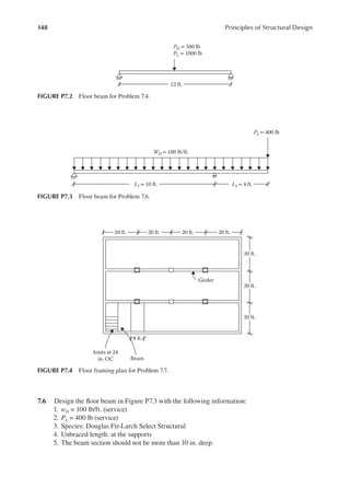
7.4 Design the loor beam in Figure P7.2 for the following conditions:
1. Span, L = 12 ft.
2. PD = 500 lb (service)
3. PL = 1000 lb (service)
4. Unbraced length: one-half of the span
5. Species: Hem Fir #1
7.5 Design the beam in Problem 7.4 for the unbraced length equal to the span.
12 ft.
12
4
FIGURE P7.1 Roof rafters for Problem 7.3.

166. 148 Principles of Structural Design
7.6 Design the loor beam in Figure P7.3 with the following information:
1. wD = 100 lb/ft. (service)
2. PL = 400 lb (service)
3. Species: Douglas Fir-Larch Select Structural
4. Unbraced length: at the supports
5. The beam section should not be more than 10 in. deep.
L2 = 4 ft.
PL = 400 lb
L1 = 10 ft.
WD = 100 lb/ft.
FIGURE P7.3 Floor beam for Problem 7.6.
20 ft. 20 ft. 20 ft.
20 ft.
20 ft.
Girder
Beam
Joists at 24
in. OC
20 ft.
20 ft.
8 ft.
FIGURE P7.4 Floor framing plan for Problem 7.7.
12 ft.
PD = 500 lb
PL = 1000 lb
FIGURE P7.2 Floor beam for Problem 7.4.

167. 149
Flexure and Axially Loaded Wood Structures
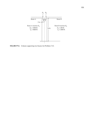
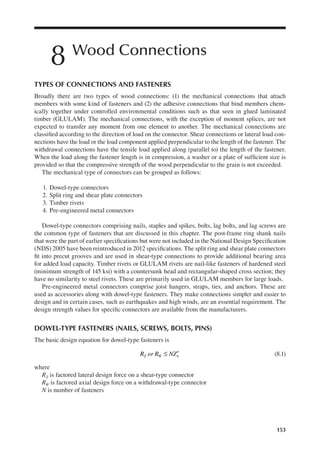
7.7 The loor framing plan of a building is shown in Figure P7.4.
Dead loads are as follows:
Floor = 12 psf
Joists = 7 psf
Beams = 9 psf
Girders = 10 psf
Live load = 40 psf
Design the beams of Southern Pine select structural timber. The beam is supported only
at the ends. The beam should not have more than 12 in. depth.
7.8 Design girders for Problem 7.7 of 24F-1.8E Southern Pine GLULAM of 63
4 in. width hav-
ing a lateral bracing at the supports only.
7.9 A Douglas Fir structural GLULAM of 24F-1.8E is used to support a loor system. The
tributary width of the beam is 12 ft. and the span is 40 ft. The dead and live loads are
15 psf and 40 psf, respectively. Design a beam of103
4 width, braced only at the supports.
7.10 To the beam shown in Figure P7.5 the loads are applied by purlins spaced at 10 ft. on
center. The beam has lateral supports at the ends and at the locations where the purlins
frame onto the beam. Design the beam of 24F-1.8E Douglas Fir GLULAM. Use 83
4-wide
section.
7.11 Design Problem 7.10. The beam is used lat with bending along the minor axis. Use
103
4-wide section.
7.12 Design the bearing plate for the supports from Problem 7.4.
7.13 Design the bearing plate for the supports from Problem 7.9.
7.14 Determine the length of the bearing plate placed under the interior loads of the beam from
Problem 7.10.
7.15 Roof trusses, spanning 24 ft. at 4 ft. on center, support a dead load of 16 psf and a snow
load of 50 psf only. The lumber is Hem Fir #1. The truss members are connected by a single
row of 3/4-in. bolts. Design the bottom chord. By truss analysis, the tensile force due to
the service loads in the bottom chord members is 5.8 k. Assume the dry wood and normal
temperature conditions.
[Hint: Divide the force in the chord between dead and snow loads in the above ratio of unit
loads for factored load determination.]
7.16 A Warren-type truss supports only dead load. The lumber is Douglas Fir-Larch #2. The
end connection consists of two rows of 1/2-in. bolts. Determine the size of the tensile mem-
ber. By truss analysis, the maximum force due to service load in the bottom chord is 5.56 k
tension. Assume dry wood and normal temperature conditions.
7.17 Design a simply supported 10-ft.-long column using Douglas Fir-Larch #1. The loads com-
prise 10 k of dead load and 10 k of roof live load.
7.18 Design a 12-ft.-long simply supported column of Southern Pine #2. The axial loads are
dead load = 1000 lb, live load = 2000 lb, and snow load = 2200 lb.
7.19 Design the column from Problem 7.18. A full support is provided by the sheeting about the
smaller dimension.
2.0 k SL
10 ft. 10 ft. 10 ft.
1.0 k DL
4.0 k SL
1.0 k DL
4.0 k SL
1.0 k DL
2.0 k SL
1.0 k DL
FIGURE P7.5 Load on beam by purlins for Problem 7.10.

168. 150 Principles of Structural Design
7.20 What is the largest axial load that can be applied to a 4 in. × 6 in. #1 Hem Fir Column? The
column is 15 ft. long, ixed at the both ends.
7.21 A 6 in. × 8 in. column carries dead and snow loads of equal magnitude. The lumber is
Douglas Fir-Larch #1. If the unbraced length of the column, which is ixed at one end and
hinged at the other end, is 9 ft., what is the load capacity of the column?
7.22 Determine the axial compression capacity of a 20-ft.-long GLULAM 63
4 in. ×
11 in. column, hinged at both ends, of SPN1D14 Southern Pine of more than four
lamination.
7.23 Determine the capacity column from Problem 7.22. It is braced at the center in the weaker
direction.
7.24 A GLULAM column of 24F-1.8E Douglas Fir carries a dead load of 20 k and a roof live
load of 40 k. The column has a simply supported length of 20 ft. Design an 83
4 in.-wide
column.
7.25 The column in Problem 7.24 is braced along the weaker axis at 8 ft. from the top. Design
a 63
4 in.-wide column.
7.26 A 2 in. × 6 in. exterior stud wall is 12 ft. tall. The studs are 16 in. on center. The studs carry
the following vertical loads per foot horizontal distance of the wall:
Dead = 400 lb/ft.
Live = 1000 lb/ft.
Snow = 1500 lb/ft.
The sheathing provides the lateral support in the weaker direction. The lumber is Douglas
Fir-Larch #1. Check the studs. Assume a simple end support condition and that the loads
on studs act axially.
7.27 The irst loor (10 ft. high) bearing wall of a building consists of 2 in. × 6 in. studs at
16 in. on center. The following roof loads are applied: roof dead load = 10 psf, roof live
load = 20 psf, wall dead load = 5 psf, loor dead load = 7 psf, live load = 40 psf, lateral
wind load = 25 psf. The tributary width of the roof framing to the bearing wall is 8 ft. The
sheathing provides a lateral support to studs in the weaker direction. Check whether the
wall studs made of Douglas Fir-Larch #2 are adequate.
7.28 A beam column is subjected to an axial dead load of 1 k, a snow load of 0.8 k, and a lat-
eral wind load of 160 lb/ft. The column height is 10 ft. Design a beam-column of section
4 × ____ of Southern Pine #1.
7.29 A tall 20-ft.-long building column supports a dead load of 4 k and a live load of 5 k along
with a lateral wind load of 240 lb/ft. Design a beam-column of 5 in.
1
8 × ____ section made
of 2DFL2 GLULAM, more than four lamination.
7.30 A vertical 4 in. × 12 in. Southern Pine dense #1, 12-ft.-long member is embedded at the
base to provide the ixidity. The other end is free to sway without rotation along the weaker
axis and is hinged along the strong axis. The bracing about the weak axis is provided at
every 4 ft. by wall girts and only at the ends about the strong axis. The dead load of 1000 lb
and the roof live load of 4000 lb act axially. A uniform wind load of 240 lb/ft. acts along
the strong axis. The sheathing provides a continuous lateral support to the compression
side. Check the member for adequacy.
[Hint: Consider that the member is ixed at one end and has a spring support at the other
end. For such a case, take the design end bending moment to be 70% of the maximum
bending moment on the column acting like a cantilever.]
7.31 Solve Problem 7.30 when no lateral support to the compression side is provided. If a
4 in. × 12 in. section in not adequate, select a new section of a maximum 12 in. depth.
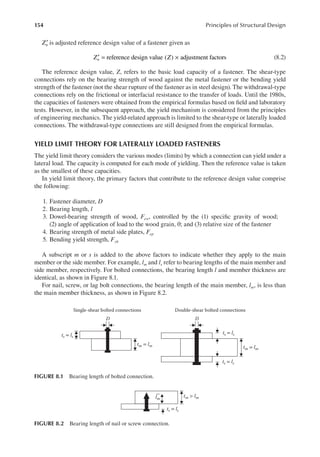
7.32 Choose a 5-in.-wide Southern Pine SPN1D14 GLULAM column supporting two beams,
as shown in Figure P7.6. The beam reactions cause bending about the major axis only. The
bottom is ixed and the top is hinged.

169. 151
Beam A Beam B
2 in.
14 ft.
Beam A reaction RA
RA RB
DL = 2000 lb
SL = 8000 lb
Beam B reaction RB
DL = 200 lb
SL = 2000 lb
FIGURE P7.6 Column supporting two beams for Problem 7.32.

171. 153
8 Wood Connections
TYPES OF CONNECTIONS AND FASTENERS
Broadly there are two types of wood connections: (1) the mechanical connections that attach
members with some kind of fasteners and (2) the adhesive connections that bind members chem-
ically together under controlled environmental conditions such as that seen in glued laminated
timber (GLULAM). The mechanical connections, with the exception of moment splices, are not
expected to transfer any moment from one element to another. The mechanical connections are
classiied according to the direction of load on the connector. Shear connections or lateral load con-
nections have the load or the load component applied perpendicular to the length of the fastener. The
withdrawal connections have the tensile load applied along (parallel to) the length of the fastener.
When the load along the fastener length is in compression, a washer or a plate of suficient size is
provided so that the compressive strength of the wood perpendicular to the grain is not exceeded.
The mechanical type of connectors can be grouped as follows:
1. Dowel-type connectors
2. Split ring and shear plate connectors
3. Timber rivets
4. Pre-engineered metal connectors
Dowel-type connectors comprising nails, staples and spikes, bolts, lag bolts, and lag screws are
the common type of fasteners that are discussed in this chapter. The post-frame ring shank nails
that were the part of earlier speciications but were not included in the National Design Speciication
(NDS) 2005 have been reintroduced in 2012 speciications. The split ring and shear plate connectors
it into precut grooves and are used in shear-type connections to provide additional bearing area
for added load capacity. Timber rivets or GLULAM rivets are nail-like fasteners of hardened steel
(minimum strength of 145 ksi) with a countersunk head and rectangular-shaped cross section; they
have no similarity to steel rivets. These are primarily used in GLULAM members for large loads.
Pre-engineered metal connectors comprise joist hangers, straps, ties, and anchors. These are
used as accessories along with dowel-type fasteners. They make connections simpler and easier to
design and in certain cases, such as earthquakes and high winds, are an essential requirement. The
design strength values for speciic connectors are available from the manufacturers.
DOWEL-TYPE FASTENERS (NAILS, SCREWS, BOLTS, PINS)
The basic design equation for dowel-type fasteners is
R or R NZ
Z W n
≤ ′ (8.1)
where
RZ is factored lateral design force on a shear-type connector
RW is factored axial design force on a withdrawal-type connector
N is number of fasteners

172. 154 Principles of Structural Design
Zn
′ is adjusted reference design value of a fastener given as
Z Z
n reference design value ( ) adjustment factors
′ = × (8.2)
The reference design value, Z, refers to the basic load capacity of a fastener. The shear-type
connections rely on the bearing strength of wood against the metal fastener or the bending yield
strength of the fastener (not the shear rupture of the fastener as in steel design). The withdrawal-type
connections rely on the frictional or interfacial resistance to the transfer of loads. Until the 1980s,
the capacities of fasteners were obtained from the empirical formulas based on ield and laboratory
tests. However, in the subsequent approach, the yield mechanism is considered from the principles
of engineering mechanics. The yield-related approach is limited to the shear-type or laterally loaded
connections. The withdrawal-type connections are still designed from the empirical formulas.
YIELD LIMIT THEORY FOR LATERALLY LOADED FASTENERS
The yield limit theory considers the various modes (limits) by which a connection can yield under a
lateral load. The capacity is computed for each mode of yielding. Then the reference value is taken
as the smallest of these capacities.
In yield limit theory, the primary factors that contribute to the reference design value comprise
the following:
1. Fastener diameter, D
2. Bearing length, l
3. Dowel-bearing strength of wood, Few, controlled by the (1) speciic gravity of wood;
(2) angle of application of load to the wood grain, θ; and (3) relative size of the fastener
4. Bearing strength of metal side plates, Fep
5. Bending yield strength, Fyb
A subscript m or s is added to the above factors to indicate whether they apply to the main
member or the side member. For example, lm and ls refer to bearing lengths of the main member and
side member, respectively. For bolted connections, the bearing length l and member thickness are
identical, as shown in Figure 8.1.
For nail, screw, or lag bolt connections, the bearing length of the main member, lm, is less than
the main member thickness, as shown in Figure 8.2.
Single-shear bolted connections
ts = ls
D
tm = lm
Double-shear bolted connections
ts = ls
ts = ls
D
tm = lm
FIGURE 8.1 Bearing length of bolted connection.
tm > lm
lm
ts = ls
FIGURE 8.2 Bearing length of nail or screw connection.

173. 155
Wood Connections
Depending on the mode of yielding, one of the strength terms corresponding to items 3, 4, or 5
above or their combinations are the controlling factor(s) for the capacity of the fastener. For exam-
ple, in the bearing-dominated yield of the wood ibers in contact with the fastener, the term Few
for wood will be a controlling factor; for a metal side member used in a connection, the bearing
strength of metal plate Fep will control.
For a fastener yielding in bending with the localized crushing of the wood ibers, both Fyb and
Few will be the relevant factors. The various yield modes are described in the “Yield Mechanisms
and Yield Limit Equations” section.
1. The dowel-bearing strength of wood, also known as the embedded strength, Few (item 3
above), is the crushing strength of the wood member. Its value depends on the speciic
gravity of wood. For large-diameter fasteners (≥1/4 in.), the bearing strength also depends
on the angle of load to grains of wood. The NDS provides the values of speciic gravity, G,
for various species and their combinations and also includes the formulas and tables for the
dowel-bearing strength, Few, for the two cases of loading—the load acting parallel to the
grains and the load applied perpendicular to the grains.
2. The bearing strength of steel members (item 4 above) is based on the ultimate tensile
strength of steel. For hot-rolled steel members (usually of thickness ≥1/4 in.), Fep = 1.5 Fu,
and for cold-formed steel members (usually <1/4 in.), Fep = 1.375 Fu.
3. The fastener bending yield strength, Fyb (item 5 above), has been listed by the NDS for
various types and diameters of fasteners. These values can be used in the absence of the
manufacturer’s data.
YIELD MECHANISMS AND YIELD LIMIT EQUATIONS
Dowel-type fasteners have the following four possible modes of yielding:
Mode I: Bearing yield of wood ibers when stress distribution is uniform over the entire thickness
of the member.
In this case, due to the high lateral loading, the dowel-bearing stress of a wood member uniformly
exceeds the strength of wood. This mode is classiied as Im if the bearing strength is exceeded in the
main member and as Is if the side member is overstressed, as shown in Figure 8.3.
Mode II: Bearing yield of wood by crushing due to maximum stress near the outer ibers.
The bearing strength of wood is exceeded in this case also. However, the bearing stress is not
uniform. In this mode, the fastener remains straight but undergoes a twist that causes lexure-like
nonuniform distribution of stress with the maximum stress at the outer ibers. The wood ibers are
accordingly crushed at the outside face of both members, as shown in Figure 8.4.
Single-shear connections
Mode Im
Mode Is
Double-shear connections
FIGURE 8.3 Mode I yielding. (Courtesy of American Forest & Paper Association, Washington, DC.)

174. 156 Principles of Structural Design
Mode II yield occurs simultaneously in the main and side members. It is not applicable to a
double-shear connection because of symmetry by the two side plates.
Mode III: Fastener bends at one point within a member and wood ibers in contact with the fas-
tener yield in bearing.
This is classiied as IIIm when fastener bending occurs and the wood bearing strength is exceeded
in the main member. Likewise, IIIs indicates the bending and crushing of wood ibers in the side
member, as shown in Figure 8.5.
Mode IIIm is not applicable to a double-shear connection because of symmetry by the two side
plates.
Mode IV: Fastener bends at two points in each shear plane and wood ibers yield in bearing near
the shear plane(s).
Mode IV occurs simultaneously in the main and side members in a single shear, as shown in
Figure 8.6. However, in a double shear, this can occur in each plane, hence yielding can occur sepa-
rately in the main member and the side member.
To summarize, in a single-shear connection, there are six modes of failures comprising Im, Is, II,
IIIm, IIIs, and IV. Correspondingly, there are six yield limit equations derived for the single-shear
connections. For a double-shear connection, there are four modes of failures comprising Im, Is, IVm,
and IVs. There are four corresponding yield limit equations for the double-shear connections.
Single-shear connection Double-shear connection
Mode II (Not applicable)
FIGURE 8.4 Mode II yielding. (Courtesy of American Forest & Paper Association, Washington, DC.)
Single-shear connection Double-shear connection
Mode IIIm
Mode IIIs
(not applicable)
FIGURE 8.5 Mode III yielding. (Courtesy of American Forest & Paper Association, Washington, DC.)
Single-shear connection Double-shear connection
Mode IV
FIGURE 8.6 Mode IV yielding. (Courtesy of American Forest & Paper Association, Washington, DC.)

175. 157
Wood Connections
REFERENCE DESIGN VALUES FOR LATERAL LOADS (SHEAR CONNECTIONS)
For a given joint coniguration, depending upon the single or the double-shear connection, six or
four yield limit equations are evaluated and the smallest value obtained from these equations is used
as a reference design value, Z.
Instead of using the yield limit equations, the NDS provides the tables for the reference design
values that evaluate all relevant equations and adopts the smallest values for various fastener
properties and speciic gravity of species. The selected reference design values for the lateral
loading are included in Appendix B, Tables B.10, B.12, B.14, B.16, and B.17 for different types of
fasteners.
As stated above under the dowel-bearing strength of wood for fasteners of 1/4 in. or larger, the
angle of loading with respect to the wood grains also affects the reference design values. The NDS
tables include two cases: one for the loads parallel to the grains and one for the loads perpendicular
to the grains. The loads that act at other angles involve the application of Hankinson formula, which
has not been considered in this book.
A reference design value, Z, obtained by the yield limit equations or from the NDS tables, is
then subjected to the adjustment factors to get the adjusted reference design value, Zn
′, to be used
in Equation 8.1. The adjustment factors are discussed in the “Adjustments of the Reference Design
Values” section.
REFERENCE DESIGN VALUES FOR WITHDRAWAL LOADS
Dowel-type fasteners are much less stronger in withdrawal capacity. The reference design values
for different types of fasteners in lb/in. of penetration is given by the empirical formulas, which are
functions of the speciic gravity of species and the diameter of the fasteners. The NDS provides
the tables based on these formulas. The selected reference design values for withdrawal loading
are included in the Appendix B, Tables B.11, B.13, B.15, B.18 for different types of fasteners.
ADJUSTMENTS OF THE REFERENCE DESIGN VALUES
Table 8.1 speciies the adjustment factors that apply to the lateral loads and withdrawal loads for
dowel-type fasteners.
The last three factors, KF, ϕz, and λ, are relevant to load resistance factor design (LRFD) only.
For connections, their values are
KF = 3.32
ϕz = 0.65
λ = as given in the “Time Effect Factor, λ” section in Chapter 6
The other factors are discussed below.
TABLE 8.1
Adjustment Factors for Dowel-Type Fasteners
LRFD Only Factors
Loads
Format
Conversion
Resistance
Factor
Time
Effect
Wet
Service Temperature
Group
Action Geometry
End
Grain Diaphragm Toenail
Lateral loads KF ϕz λ CM Ct Cg CΔ Ceg Cdi
a Ctn
a
Withdrawal KF ϕz λ CM Ct — — Ceg — Ctn
a
a This factor applies to nails and spikes only.

176. 158 Principles of Structural Design
WET SERVICE FACTOR, CM
For connections, the listed reference design values are for seasoned wood having a moisture con-
tent of 19% or less. For wet woods or those exposed to wet conditions, the multiplying factors of
less than 1 are speciied in the NDS Table 10.3.3 of the National Design Speciication for Wood
Construction cited in the Bibliography.
TEMPERATURE FACTOR, Ct
For connections that will experience sustained exposure to higher than 100°F temperature, a fac-
tor of less than 1 shall be applied, as speciied in the NDS Table 10.3.4 of the National Design
Speciication for Wood Construction cited in the Bibliography.
GROUP ACTION FACTOR, Cg
A row of fasteners consists of a number of fasteners in a line parallel to the direction of loading. The
load carried by fasteners in a row is not equally divided among the fasteners; the end fasteners in a
row carry a larger portion of the load as compared to the interior fasteners. The unequal sharing of
loads is accounted for by the group action factor, Cg.
For dowel-type fasteners of diameter less than 1/4 in. (i.e., nails and wood screws), Cg = 1. For
1/4 in. or larger diameter fasteners, Cg is given by a formula, which is quite involved. The NDS provides
tabulated values for simpliied connections. The number of fasteners in a single row is the primary
consideration. For bolts and lag screws, conservatively, Cg has the values indicated in Table 8.2 (nails
and screws have Cg = 1).
GEOMETRY FACTOR, C∆
When the diameter of a fastener is less than 1/4 in. (nails and screws), C∆∆ = 1. For larger diameter
fasteners, the geometry factor accounts for the end distance, edge distance, and spacing of fasteners,
as deined in Figure 8.7.
1. The edge distance requirements, according to the NDS, are given in Table 8.3, where l/D
is the lesser of the following:
a.
bearinglengthof boltinmainmember
boltdiameter
l
D
m
=
b.
combined bearinglengthof boltinallsidemembers
boltdiameter
l
D
s
=
2. The spacing requirements between rows, according to the NDS, are given in Table 8.4,
where l/D is deined above.
3. The end distance requirements, according to the NDS, are given in Table 8.5.
4. The spacing requirements for fasteners along a row, according to the NDS, are given in
Table 8.6.
TABLE 8.2
Conservative Value of the Group Action Factor
Number of Fasteners in One Row cg
2 0.97
3 0.89
4 0.80

177. 159
Wood Connections
The provisions for C∆ are based on the assumption that the edge distance and the spacing between
rows are met in accordance with Tables 8.3 and 8.4, respectively. In addition, the perpendicular to
grain distance between the outermost fastener rows should not exceed 5 in. for sawn lumber and
GLULAM with CM = 1.
Spacing between
bolts in a row
Spacing between
bolts in a row
Spacing between
rows of bolts
Parallel-to-grain loading
Loaded
edge
distance
Unloaded
edge distance
Row
Row
Perpendicular-to-grain loading
Edge distance
Spacing between
rows of bolts
End distance
FIGURE 8.7 Connection geometry. (Courtesy of American Forest & Paper Association, Washington, DC.)
TABLE 8.3
Minimum Edge Distance
Direction of Loading Minimum Edge Distance
1. Parallel to grains
When l/D ≤ 6 1.5D
When l/D > 6 1.5D or 1/2 spacing between rows, whichever is greater
2. Perpendicular to grains
Loaded edge 4D
Unloaded edge 1.5D

178. 160 Principles of Structural Design
The requirements for the end distance and the spacing along a row for C∆ = 1 are given in the
second column of Tables 8.5 and 8.6. The tables also indicate the (absolute) minimum requirements
that must be provided for. When the actual end distance and the actual spacing along a row are less
than those indicated for C∆ = 1, the value of C∆ should be computed by the following ratio:
actual end distance or actual spacing along a row
end distance for 1from Table 8.5 or spacing 1from Table 8.6
C
C C
=
= =
For fasteners located at an angle, the geometry factor, C∆, also depends on the shear area.
For C∆ to be 1, the minimum shear area of an angled member as shown in Figure 8.8 should be
equal to the shear area of a parallel member connection having the minimum end distance as
required for C∆ = 1 from Table 8.5 as shown in Figure 8.9. If the angled shear area is less, the
geometry factor C∆ is determined by the ratio of the actual shear area to that required for C∆ = 1
from Figure 8.9.
The geometry factor is the smallest value determined from the consideration of the end distance,
spacing along the row, and the angled shear area.
TABLE 8.4
Minimum Spacing between Rows
Direction of Loading Minimum Spacing
1. Parallel to grains 1.5D
2. Perpendicular to grains
When l/D ≤ 2 2.5D
When l/D > 2 but <6 (5l + 10D)/8
When l/D ≥ 6 5D
TABLE 8.5
Minimum End Distance
Direction of Loading End Distance for c∆ = 1 Minimum End Distance for c∆ = 0.5
1. Parallel to grains
Compression 4D 2D
Tension—softwood 7D 3.5D
Tension—hardwood 5D 2.5D
2. Perpendicular to grains 4D 2D
TABLE 8.6
Minimum Spacing in a Row
Direction of Loading Spacing for c∆ = 1 Minimum Spacing
1. Parallel to grains 4D 3D
2. Perpendicular to grains On side plates (attached member) spacing
should be 4D
3D

179. 161
Wood Connections
END GRAIN FACTOR, Ceg
In a shear connection, load is perpendicular to the length (axis) of the fastener, and in a withdrawal
connection, load is parallel to the length of the fastener. But in both cases, the length (axis) of the
fastener is perpendicular to the wood ibers (fastener is installed in the side grains). However, when
a fastener penetrates an end grain so that the fastener axis is parallel to the wood ibers, as shown in
Figure 8.10, it is a weaker connection.
For a withdrawal-type loading, Ceg = 0.75. For a lateral (shear)-type loading, Ceg = 0.67.
DIAPHRAGM FACTOR, Cdi
This applies to nails and spikes only. When nails or spikes are used in diaphragm construction,
Cdi = 1.1.
TOENAIL FACTOR, Ctn
This applies to nails and spikes only. In many situations, it is not possible to directly nail a side mem-
ber to a holding member. Toenails are used in the side member at an angle of about 30° and start
at about 1/3 of the nail length from the intersection of the two members, as shown in Figure 8.11.
For lateral loads, Ctn = 0.83. For withdrawal loads, Ctn = 0.67. For withdrawal loads, the wet-
service factor is not applied together with Ctn.
Shear area
FIGURE 8.8 Shear area for fastener loaded at angle.
Shear area
Minimum end distance for CΔ = 1
FIGURE 8.9 Shear area of parallel member connection.
FIGURE 8.10 End grain factor.

180. 162 Principles of Structural Design
Example 8.1
The reference lateral design value for the parallel-to-grain loaded lag screw connection shown
in Figure 8.12 is 1110 lb. Determine the adjusted reference design value. The diameter of screws
is 7/8 in. The connection is subjected to dead and live tensile loads in dry softwood at normal
temperatures.
SOLUTION
1. Adjusted reference design value, Zn
′ = Z × (ϕzλCgCΔKF); since CM and Ct = 1
2. ϕz = 0.65
3. λ = 0.8
4. KF = 3.32
5. Group action factor, Cg
For three fasteners in a row, Cg = 0.89 (from Table 8.2)
6. Geometry factor, CΔ
a. End distance = 4 in.
b. End distance for CΔ = 1, =





 =
D
7 7
7
8
6.125in.
c. = = ←
End factor
4.0
6.125
0.65 controls
d. Spacing along a row = 3 in.
e. Spacing for CΔ = 1, 4D = 3.5 in.
f. Spacing factor
3.0
3.5
0.857
= =
7. ′ = =
Zn 1110(0.65)(0.8)(0.89)(0.65)(3.32) 1108.6 lb
1½ in.
1½ in.
3 in.
4 in. 3 in.
Direction of
loading
7
8
in.
FIGURE 8.12 Parallel-to-grain loaded connection.
L
L/3
30°
FIGURE 8.11 Toenail factor.

181. 163
Wood Connections
Example 8.2
The reference lateral design value for the perpendicular-to-grain loaded bolted connection shown in
Figure 8.13 is 740 lb. Determine the adjusted reference design value. The bolt diameter is 7/8 in. Use
soft dry wood and normal temperature conditions. The connection is subjected to dead and live loads.
SOLUTION
1. Adjusted reference design value, Zn
′ = Z × (ϕzλCgCΔKF); since CM and Ct = 1
2. ϕz = 0.65
3. λ = 0.8
4. KF = 3.32
5. Group action factor, Cg
For two fasteners in a row, Cg = 0.97 (from Table 8.2)
6. Geometry factor, CΔ
a. End distance = 2 in.
b. End distance for CΔ = 1, 4D = 4
7
8





 = 3.5 in.
c. End factor
2.0
3.5
0.57 controls
= = ←
d. Spacing along a row = 3 in.
e. Spacing for CΔ = 1, 4D = 4
7
8





 = 3.5 in.
f. Spacing factor
3.0
3.5
0.857
= =
7. 740(0.65)(0.80)(0.97)(0.57)(3.32) 706.3 lb
Zn
′ = =
Example 8.3
The connection of Example 8.1 when loaded in withdrawal mode has a reference design value of
500 lb. Determine the adjusted reference withdrawal design value.
SOLUTION
1. Adjusted reference design value, Zn
′ = Z × (ϕzλKF);
2. ϕz = 0.65
3. λ = 0.8
4. KF = 3.32
5. Zn 500(0.65)(0.80)(3.32) 863 lb
′ = =
3 in.
Direction of loading
7
8
in. bolts
2 in.
2 in.
3 in.
3½ in.
FIGURE 8.13 Perpendicular-to-grain loaded connection.

182. 164 Principles of Structural Design
NAIL AND SCREW CONNECTIONS
Once the adjusted reference design value is determined, Equation 8.1 can be used with the factored
load to design a connection for any dowel-type fasteners. Nails and wood screws generally fall
into small-size fasteners having a diameter of less than 1/4 in. For small-size fasteners, the angle
of load with respect to grains of wood is not important. Moreover, the group action factor, Cg, and
the geometry factor, CΔ, are not applicable. The end grain factor, Ceg, the diaphragm factor, Cdi, and
the toenail factor, Ctn, apply to speciic cases. Thus, for a common type of dry wood under normal
temperature conditions, no adjustment factors are required except for the special LRFD factors of
ϕz, λ, and KF.
The basic properties of nails and wood screws are described below.
COMMON, BOX, AND SINKER NAILS
Nails are speciied by the pennyweight, abbreviated as d. A nail of a speciic pennyweight has a
ixed length, L, shank diameter, D, and head size, H. There are three kinds of nails: common, box,
and sinker. Common and box nails have a lat head and sinker nails have a countersunk head, as
shown in Figure 8.14.
For the same pennyweight, box and sinker nails have a smaller diameter and, hence, a lower
capacity as compared to common nails.
ThereferencelateraldesignvaluesforthesimplenailconnectoraregiveninAppendixB,TableB.10.
The values for the other cases are included in the NDS speciications. The reference withdrawal design
values for nails of different sizes for various wood species are given in Appendix B, Table B.11.
POST-FRAME RING SHANK NAILS
These are threaded nails. There are two types of threads. In annular nails, the threads are perpendic-
ular to the nail axis. The threads of helical nails are aligned at an angle between 30° and 70° to the
nail axis. The annular nails are called the post-frame ring shank nails, as shown in Figure 8.15. The
threaded nails have higher withdrawal strength because of wood ibers lodged between the threads.
The typical dimensions of post-frame ring shank nails are given in Table 8.7. The reference design
values for post-frame ring shank nails using a single-shear connection are given in Appendix B,
Table B.12. The reference withdrawal design values per inch penetration are given in Appendix B,
Table B.13.
L
D
H
Common or box
Sinker
H
D = Diameter
L =Length
H= Head diameter
L
D
FIGURE 8.14 Typical speciications of nails.

183. 165
Wood Connections
WOOD SCREWS
Wood screws are identiied by a number. A screw of a speciic number has a ixed diameter (outside
to outside of threads) and a ixed root diameter, as shown in Figure 8.16. Screws of each speciic
number are available in different lengths. There are two types of screws: cut thread screws and
rolled thread screws. The thread length, T, of a cut thread screw is approximately 2/3 of the screw
length, L. In a rolled thread screw, the thread length, T, is at least four times the screw diameter, D,
or 2/3 of the screw length, L, whichever is greater. The screws that are too short to accommodate
the minimum thread length have threads extended as close to the underside of the head as practical.
The screws are inserted in their lead hole by turning with a screwdriver; they are not driven by
a hammer. The minimum penetration of the wood screw into the main member for single shear or
into the side member for double shear should be six times the diameter of the screw. Wood screws
are not permitted to be used in a withdrawal-type connection in end grain.
The reference lateral design values for simple wood screw connections are given in Appendix B,
Table B.14. The values for other cases are included in the NDS speciications. The reference with-
drawal design values for wood screws are given in Appendix B, Table B.15.
T1
D
H
P
L
TL
FIGURE 8.15 Typical speciications of post-frame ring shank nails.
TABLE 8.7
Typical Dimensions of Post-Frame Ring Shank Nails
D (in.) L (in.) H (in.) Root Diameter, Dr (in.)
0.135 3, 3.5 5/16 0.128
0.148 3, 3.5, 4, 4.5 5/16 0.140
0.177 3, 3.5, 4, 4.5, 5, 6, 8 3/8 0.169
0.20 3.5, 4, 4.5, 5, 6, 8 15/32 0.193
0.207 4, 4.5, 5, 6, 8 15/32 0.199
Cut thread
Rolled thread
L
T
Dr D
L
T
Dr D
D = Diameter
Dr= Root diameter
L = Screw length
T =Thread length
FIGURE 8.16 Typical speciications of wood screws.

184. 166 Principles of Structural Design
Example 8.4
A 2 in. × 6 in. diagonal member of No. 1 Southern Pine is connected to a 4 in. × 6 in. column, as
shown in Figure 8.17. It is acted upon by a service wind load component of 2 k. Design the nailed
connection. Neglect the dead load.
SOLUTION
1. Factored design load, RZ = 1(2) = 2 k or 2000 lb
2. Use 30d nails, 3 in a row
3. Reference design value for a side thickness of 1.5 in.
From Appendix B, Table B.10, Z = 203 lb
4. For nails, the adjusted reference design value
Z Z K
n z F
( )
′ = × φ λ
where
ϕz = 0.65
λ = 1.00
KF = 3.32
203(0.65)(1)(3.32) 438lb
Zn
′ = =
5. From Equation 8.1
Z
z
n
N
R 2000
438
4.57 nails
=
′
= =
6. For number of nails per row, n = 3
Number of rows
4.57
3
1
.52 (use 2)
= =
Provide 2 rows of 3 nails each of 30d size
BOLT AND LAG SCREW CONNECTIONS
Bolts and lag screws are used for larger loads. The angle of load to grains is an important consider-
ation in large diameter (≥1/4 in.) connections comprising bolts and lag screws. However, this book
makes use of the reference design tables, in lieu of the yield limit equations, which include only
the two cases of parallel-to-grain and perpendicular-to-grain conditions. The group action factor,
Cg, and the geometry factor, CΔ, apply to bolts and lag screws. Although the end grain factor, Ceg,
is applicable, it is typical to a nail connection. The other two factors, the diaphragm factor, Cdi, and
the toenail factor, Ctn, also apply to nails.
An important consideration in bolt and lag screw connection design is to accommodate the num-
ber of bolts and rows within the size of the connecting member satisfying the requirements of the
end, edge, and in-between bolt spacing.
The larger diameter fasteners often involve the use of prefabricated steel accessories or hard-
ware. The NDS provides details of the typical connections involving various kinds of hardware.
Live load
Nail
connection
FIGURE 8.17 Diagonal member nail connection.

185. 167
Wood Connections
BOLTS
In steel structures, the trend is to use high-strength bolts. However, this is not the case in wood
structures where low-strength A307 bolts are commonly used. Bolt sizes used in wood construction
range from 1/2 in. through 1 in. diameter, in increments of 1/8 in. The NDS restricts the use of bolts
to a largest size of 1 in. The bolts are installed in the predrilled holes. The NDS speciies that the
hole size should be a minimum of 1/32 in. to a maximum of 1/16 in. larger than the bolt diameter
for uniform development of the bearing stress.
Most bolts are used in the lateral-type connections. They are distinguished by the single-shear
(two members) and double-shear (three members) connections. For more than double shear, the
single-shear capacity at each shear plane is determined and the value of the weakest shear plane is
multiplied by the number of shear planes.
The connections are further recognized by the types of main and side members, such as wood-
to-wood, wood-to-metal, wood-to-concrete, and wood-to-masonry connections. The last two are
simply termed as anchored connections.
Washers of adequate size are provided between the wood member and the bolt head, and between
the wood member and the nut. The size of the washer is not of signiicance in shear. For bolts in
tension and compression, the size should be adequate so that the bearing stress is within the com-
pression strength perpendicular to the wood grain.
The reference lateral design values for a simple bolted connection are given in Appendix B,
Table B.16
LAG SCREWS
Lag screws are relatively larger than wood screws. They have wood screw threads and a square or
hexagonal bolt head. The dimensions for lag screws include the nominal length, L; diameter, D; root
diameter, Dr; unthreaded shank length, S; minimum thread length, T; length of tapered tip, E; num-
ber of threads per in., N; height of head, H; and width of head across lats, F, as shown in Figure 8.18.
Lag screws are used when an excessive length of bolt will be required to access the other side or
when the other side of a through-bolted connection is not accessible. Lag screws are used in shear
as well as in withdrawal applications.
Lag screws are installed with a wrench as opposed to wood screws, which are installed by screw-
drivers. Lag screws involved pre-bored holes with two different diameter bits. The larger diameter
hole has the same diameter and length as the unthreaded shank of the lag screw and the lead hole
for the threaded portion is similar to that for wood screw, the size of which depends on the speciic
gravity of the wood. The minimum penetration (excluding the length of the tapered tip) into the
main member for single shear and into the side member for double shear should be four times the
lag screw diameter, D.
The reference lateral design values for simple lag screw connection are given in Appendix B,
Table B.17. The other cases are included in the NDS speciications. The reference withdrawal design
values for lag screws are given in Appendix B, Table B.18.
Dr D
L
H
E
T–E
S
F
S =Unthreaded shank length
T= Minimum thread length
E=Length of tapered tip
N= Number of threads/inch
FIGURE 8.18 Typical speciications of log screws.

186. 168 Principles of Structural Design
Example 8.5
The diagonal member of Example 8.4 is subjected to a wind load component of 4 k. Design the
bolted connection. Use 5/8-in. bolts.
SOLUTION
1. Factored design load, RZ = 1(4) = 4 k or 4000 lb
2. Use 5/8-in. bolts, two in a row
3. Reference design value
a. For a side thickness of 1.5 in.
b. Main member thickness of 3.5 in.
c. From Appendix B, Table B.16, Z = 940 lb
4. Adjusted reference design value, Z Z C C K
n Z g F
( )
′ = × φ λ
5. ϕz = 0.65
λ = 1.0
KF = 3.22
6. Group action factor, Cg
For two fasteners in a row, Cg = 0.97 (from Table 8.2)
7. Geometry factor, C∆
a. End distance to accommodate within 6 in. column size = 2.5 in.
b. Spacing within 6 in. column = 2 in.
c. End distance for C∆ = 1, 7D = 4.375 in.
d. End factor
2.5
4.375
0.57 controls
= = ←
e. Spacing CΔ = 1, 4D = 2.5 in.
f. Spacing factor
2
2.5
0.8
= =
8. 940(0.65)(1)(0.97)(0.57)(3.22) 1087.8 lb
Zn
′ = =
9. From Equation 8.1
Z
z
n
N
R 4000
1087.8
3.7
=
′
= =
10. Number of bolts per row, n = 2
Number of rows
3.7
2
1
.85 use 2
( )
= =
Provide 2 rows of two 5/8-in. bolts
PROBLEMS
8.1 The reference lateral design value of a parallel-to-grain loaded lag screw connection
shown in Figure P8.1 is 740 lb. The screw diameter is 5/8 in. The loads comprise dead
and live loads. Determine the adjusted reference design value for soft dry wood at normal
temperature.
8.2 The reference lateral design value of a perpendicular-to-grain loaded lag screw connection
shown in Figure P8.2 is 500 lb. The screw diameter is 5/8 in. The loads comprise dead
and live loads. Determine the adjusted reference design value for soft dry wood at normal
temperature.
8.3 The connection in Problem 8.1 has a reference withdrawal design value of 400 lb. Determine
the adjusted reference design value.
8.4 Problem 8.2 is a nailed connection by 0.225-in.-diameter nails. The holding member has
ibers parallel to the nail axis. The reference design value is 230 lb. Determine the adjusted
reference design value.

187. 169
Wood Connections
8.5 A spliced parallel-to-grain-loaded connection uses two rows of 7/8-in. lag screws with
three fasteners in each row, as shown in Figure P8.3. The load carried is 1.2D + 1.6L. The
reference design value is 1500 lb. The connection is in hard dry wood at normal tempera-
ture. Determine the adjusted reference design value.
8.6 The connection in Problem 8.5 is subjected to a perpendicular-to-grain load from the
top only. The reference design value is 1000 lb. Determine the adjusted reference design
value.
8.7 The connection in Problem 8.5 is subjected to withdrawal loading. The reference design
value is 500 lb. Determine the adjusted reference design value.
8.8 The connection shown in Figure P8.4 uses 3/4-in.-diameter bolts in a single shear. There
are two bolts in each row. The reference design value is 2000 lb. It is subjected to lateral
wind load only (no live load). Determine the adjusted reference design value for soft dry
wood at normal temperature.
8.9 For the connection shown in Figure P8.5, the reference design value is 1000 lb. Determine
the adjusted reference design value for dry wood under normal temperature conditions.
8.10 Toenails of 50d pennyweight (0.244 in. diameter, 5½ in. length) are used to connect a
beam to the top plate of a stud wall, as shown in Figure P8.6. It is subjected to dead
and live loads. The lateral reference design value is 250 lb. Determine the adjusted refer-
ence design value for soft wood under normal temperature and dry conditions. Show the
connection.
2 in.
2 in.
2 in.
1 in.
2 in.
1 in.
2 in.
1
2
FIGURE P8.1 Parallel-to-grain screw connection for Problem 8.1.
2 in.
2.5 in.
2 in.
1 in.
2 in.
1.5in.
FIGURE P8.2 Perpendicular-to-grain screw connection for Problem 8.2.

188. 170 Principles of Structural Design
3 in.
3 in.
FIGURE P8.4 A single shear connection.
3 in.
4 in.
4 in.
(Snow load)
3 in.
1½ in.
1-in.-dia bolts
PD
PS
+
+
+
–
FIGURE P8.5 Perpendicular-to-grain bolted connection for Problem 8.9.
Stud
Wall plate
4 in. × 10 in.
beam
FIGURE P8.6 Toenail connection to a top plate.
3 in. 3 in.
2.5in.
+
+
+
+
+
+
+
+
+
+
+
+
1.5 in.
1.5 in.
3 in.
FIGURE P8.3 Spliced parallel-to-grain connection.

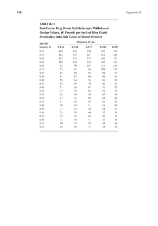
189. 171
Wood Connections
8.11 Design a nail connection to transfer tensile service dead and live loads of 400 and 600 lb,
respectively, acting along the axis of a 2 in. × 6 in. diagonal member connected to a 4 in. ×
4 in. vertical member. Use No. 1 Southern Pine soft dry wood. Assume two rows of 30d
common nails.
8.12 A 2 in. × 8 in. diagonal member is connected by 20d common nails to a 4 in. × 6 in. verti-
cal member. It is acted upon by a combined factored dead and snow load of 1.5 k. Design
the connection. Use Douglas Fir-Larch dry wood (G = 0.5).
8.13 Determine the tensile capacity of a spliced connection acted upon by the dead and snow
loads. The joint connects two 2 in. × 6 in. No. 1 Southern Pine members together by 10d
common nails via one side plate of 1 in. thickness, as shown in Figure P8.7.
8.14 Two 2 in. × 8 in. members of Douglas Fir-Larch (G = 0.5) are to be spliced connected via
a single 1½-in.-thick plate on top with two rows of #9 size screws. The service loads com-
prise 200 lb of dead load and 500 lb of live load that act normal to the ibers. Design the
connection.
8.15 Southern Pine #1, 10-ft.-long 2 in. × 4 in. wall studs, spaced at 16 in. on center (OC) are
toenailed on to Southern Pine #1 top and bottom plates with two 10d nails at each end. The
horizontal service wind load of 30 psf acts on the studs. Is the connection adequate?
8.16 The service dead load and live load in Problem 8.11 are doubled. Design a lag screw con-
nection using. 1/2-in.-lag screws. Assume the edge distance, end distance, and bolt spacing
along the diagonal of 2 in. each.
[Hint: Only two bolts per row can be arranged along the diagonal within a 4 × 4 column
size.]
8.17 A 2 in. × 6 in. is connected to a 4 in. × 6 in. member, as shown in Figure P8.8. Design
a 1/2 in. lag screw connection to transfer the dead and snow (service) loads of 0.4 k and
1.2 k, respectively. The wood is soft Hem Fir-Larch No. 1 in dry conditions at normal
temperature.
[Hint: For a beam size of 6 in., only three bolts can be arranged per row of the vertical
member.]
PD
PS (Snow)
+
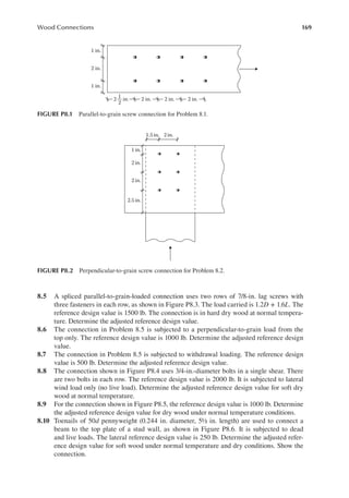
FIGURE P8.7 A spliced nail connection.
2 in. × 6 in.
4 in. × 6 in.
PS (Snow)
2 in. × 6 in.
4 in. × 6 in. 6 in.
FIGURE P8.8 A beam–column shear connection.

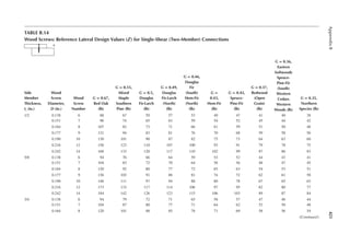
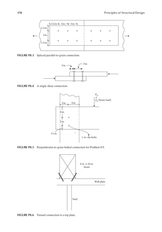
190. 172 Principles of Structural Design
8.18 Determine the number and placement of 5/8-in. bolts to transfer the service dead and snow
loads of 0.2 k and 2.85 k, respectively, through a joint, as shown in Figure P8.9. The single
shear reference design value is 830 lb, which should be doubled for two shear planes.
8.19 The controlling load on the structural member in Problem 8.17 is an unfactored wind load
of 3.2 k that acts horizontally. Design the 1/2-in. bolted connection.
[Hint: Load acts normal to the grain and three rows can be arranged within the column
size for the horizontally acting load.]
8.20 The main members of 3 in. × 10 in. are spliced connected by one 2 in. × 10 in. side member
of Southern Pine #1 soft dry wood. The connection consists of six 1-in. bolts in two rows in
each splice. Determine the joint capacity for dead and live loads. The end distance and bolt
spacing are 3.5 in. each. If the dead load is one-half of the live load, what is the magnitude
of each load?
2–2 in. × 6 in.
Southern Pine #1
6 in. × 10 in.
Item Fir #1
FIGURE P8.9 A beam–column double-shear connection.

191. Section III
Steel Structures

193. 175
9 Tension Steel Members
PROPERTIES OF STEEL
Steel structures commonly consist of frames, cables and trusses, and plated structures. The bracing
in the form of diagonal members provides the lateral stiffness. For steel elements, generally, the stan-
dard shapes, which are speciied according to the American Society of Testing Materials (ASTM)
standards, are used. The properties of these elements are listed in the beginning of the manual of the
AmericanInstituteofSteelConstruction(AISC)underDimensionsandPropertiessection.Acommon
element is an I-shaped section having horizontal langes that are connected at the top and bottom of
a vertical web. This type of section is classiied into W, M, S, and HP shapes, the difference in these
shapes essentially being in the width and thickness of langes. A typical designation “W14 × 68”
means a wide lange section having a nominal depth of 14 in. and a weight of 68 lb/ft. of length. The
other standard shapes are channels (C and MC), angles (∟), and tees (WT, MT, and ST).
Tubular shapes are common for compression members. The rectangular and square sections are
designated by the letters HSS along with the outer dimensions and the wall thickness. The round
tubing is designated as HSS round (for Grade 42) and pipes (for Grade 35) along with the outer
diameter and the wall thickness. The geometric properties of the frequently used wide lange sec-
tions are given in Appendix C, Table C.1a and b, with those for channel sections in Appendix C,
TableC.2aandb,anglesectionsinAppendixC,TableC.3athroughc,rectangulartubinginAppendixC,
Table C.4a and b, square tubing in Appendix C, Table C.5, round tubing in Appendix C, Table C.6,
and pipes in Appendix C, Table C.7.
The structural shapes are available in many grades of steel classiied according to the ASTM
speciications. The commonly used grades of steel for various structural shapes are listed in
Table 9.1.
The yield strength is a very important property of steel because so many design procedures are
based on this value. For all grades of steel, the modulus of elasticity is practically the same at a level
of 29 × 103 ksi, which means the stress–strain relation of all grades of steel is similar.
A distinguished property that makes steel a very desirable structural material is its ductility—a
property that indicates that a structure will withstand an extensive amount of deformation under
very high level of stresses without failure.
PROVISIONS TO DESIGN STEEL STRUCTURES
The AISC Speciication for Structural Steel Buildings (AISC 360) is intended to cover common design
criteria. This document forms a part of the AISC Steel Construction Manual. However, it is not feasible
to cover within such a document all special and unique problems that are encountered within the full
range of the structural design. Accordingly, AISC 360 covers the common structures of low seismicity
and a separate AISC document, Seismic Provisions for Structural Steel Buildings (AISC 341), addresses
the high-seismic applications. The latter document is incorporated within the Seismic Design Manual.
The seismic provisions are not required for following structures, which are designed according
to AISC 360:
1. Structures in seismic design category A
2. Structures in seismic design categories B and C where the response modiication factor
(coeficient), R, is not greater than 3

194. 176 Principles of Structural Design
UNIFIED DESIGN SPECIFICATIONS
A major uniication of the codes and speciications for structural steel buildings has been
accomplished by the AISC. Formerly, the AISC provided four design publications, one separately
for the allowable stress design (ASD) method, the load resistance factor design (LRFD) method,
the single-angle members, and the hollow tubular structural sections. However, the 13th edition
of the Steel Construction Manual of AISC 2005 combined all these provisions in a single volume.
Additionally, the 2005 AISC speciications established common sets of requirements for both the
ASD and LRFD methods for analyses and designs of structural elements.
The 14th edition of the Steel Construction Manual of AISC 2010 updated the tables of element
shapes to conform to ASTM A6-09. This comprised of adding and deleting some shapes and slightly
changing some areas in some cases.
The factors unifying the two methods are as follows:
1. The nominal strength is the limiting state for failing of a steel member under different
modes like compression, tension, or bending. It is the capacity of the member. The same
nominal strength applies to both the ASD and LRFD methods of design.
2. For ASD, the available strength is the allowable strength, which is the nominal strength
divided by a factor of safety. The available strength for LRFD is the design strength, which
is the nominal strength multiplied by a resistance (uncertainty) factor.
3. The required strength for a member is given by the total of the service loads that act on the
structure for the ASD method. The required strength for the LRFD method is given by the
total of the factored (magniied) loads.
4. The required strength for loads should be within the available strength of the material.
Since the allowable strength of ASD and the design strength of LRFD are both connected with
the nominal strength as indicated in item 2, there can be a direct relationship between the factor
of safety of ASD and the resistance factor of LRFD. This was discussed in the “Working Stress
Design, Strength Design, and Uniied Design of Structures” section in Chapter 1.
LIMIT STATES OF DESIGN
All designs are based on checking that the limit states are not exceeded. For each member type
(tensile, column, beam), the AISC speciications identify the limit states that should be checked.
The limit states consider all possible modes of failures like yielding, rupture, and buckling, and also
consider the serviceability limit states like delection and slenderness.
TABLE 9.1
Common Steel Grades
ASTM Classiication
Yield Strength,
Fy (ksi)
Ultimate Strength,
Fu (ksi)
Applicable Shapes
A36 36 58 W, M, S, HP, ∟, C, MC, WT
A572 Grade 50 50 65 Same
A992 Grade 50 50 65 Same
A500 Grade B 46 58 HSS—rectangular and square
A500 Grade B 42 58 HSS—round
A53 Grade B 35 60 Pipe—round

195. 177
Tension Steel Members
The limit states design process consists of the following:
1. Determine all applicable limit states (modes of failures) for the type of member to be
designed.
2. Determine the expression for the nominal strength (and the available strength) with respect
to each limit state.
3. Determine the required strength from the consideration of the loads applied on to the
member.
4. Conigure the member size by equating items 2 and 3 of this section.
In ASD, safety is established through a safety factor, which is independent of the types of loading.
In LRFD, safety is established through a resistance factor and a load factor that varies with load
types and load combinations.
DESIGN OF TENSION MEMBERS
In the AISC Manual (2010), Chapter D of Part 16 applies to members that are subject to axial ten-
sion and Section J4 of Chapter J applies to connections and connecting elements like gusset plates
that are in tension.
The limiting states for the tensile members and the connecting elements are controlled by the
following modes:
1. Tensile strength
2. Shear strength of connection
3. Block shear strength of connection along the shear/tension failure path
The shear strength of connection (item 2) will be discussed in Chapter 13 on steel connections.
TENSILE STRENGTH OF ELEMENTS
The serviceability limit state of the slenderness ratio L/r* being less than 300 for members in
tension is not mandatory in the new speciications although Section D1 recommends this value of
300 except for rods and hangers.
The design tensile strength of a member shall be the lower of the values obtained for the limit
states of (1) the tensile yielding at the gross area and (2) the tensile rupture at the net area.
Thus, the strength is the lower of the following two values:
Based on the limit state of yielding in the gross section
=
P F A
u y g
0.9 (9.1)
Based on the limit state of rupture in the net section
=
P F A
u u e
0.75 (9.2)
where
Pu is factored design tensile load
Fy is yield strength of steel
* L is the length of the member and r is the radius of gyration given by /
I A .

196. 178 Principles of Structural Design
Fu is ultimate strength of steel
Ag is gross area of member
Ae is effective net area
In connecting members, if a portion of a member is not fully connected like a leg of an angle section,
the unconnected part is not subjected to the full stress. This is referred to as a shear leg. A factor is
used to account for the shear lag. Thus,
=
A A U
e n (9.3)
where
An is net area
U is shear lag factor
NET AREA, An
The net area is the product of the thickness and the net width of a member. To compute net width,
the sum of widths of the holes for bolts is subtracted from the gross width. The hole width is taken
as 1/8 in. greater than the bolt diameter.
For a chain of holes in a zigzag line shown as a-b in Figure 9.1, a quantity s2/4g is added to the net
width for each zigzag of the gage space, g, in the chain. Thus,
4
2
A bt ht
s
g
t
n ∑ ∑
= − +





 (9.4)
where
s is longitudinal (in the direction of loading) spacing between two consecutive holes (pitch)
g is transverse (perpendicular to force) spacing between the same two holes (gage)
b is width of member
t is thickness of member
h is size of hole
For angles, the gage for holes in the opposite legs, as shown in Figure 9.2, is g = g1 + g2 – t.
g2
g1
FIGURE 9.2 Gage for holes in angle section.
b
g
t s
a
b
FIGURE 9.1 Zigzag pattern of holes.

197. 179
Tension Steel Members
Example 9.1
An angle ∟ 5 × 5 × 1/2* has a staggered bolt pattern, as shown in Figure 9.3. The holes are for
bolts of 7/8 in. diameter. Determine the net area.
SOLUTION
1. Ag = 4.79 in.2, t = 0.5 in.
2. h = d + (1/8) = (7/8) + (1/8) = 1 in.
3. g = g1 + g2 − t = 3 + 2 – 0.5 = 4.5 in.
4. Section through line a-b-d-e: deducting for two holes
A A ht
n g
4.79 2(1)(0.5) 3.79 in.2
∑
= −
= − =
5. Section through line a-b-c-d-e: deducting for three holes and adding s2/4g for b-c and c-d
A A ht
s
g
t
s
g
t
n g
bc cd
3
4 4
4.79 3(1)(0.5)
2
4(4.5)
0.5
2
4(1.5)
0.5
3.71in. Controls
2 2
2 2
2
= − +





 +






= − +





 +






= ←
EFFECTIVE NET AREA, Ae
1. Plates with bolted connections
As the lat plates are fully in contact and the entire area participates in transmitting the
load, the shear lag factor, U = 1.
But for bolted slice plates, the net effective area should not be more than 85% of the gross
area. Thus,
= ≤
A A A
e n g
0.85 (9.5)
* Properties of this section not included in the appendix.
2 in.
a
b
d
c
g
e
2 in.
2 in.
1 in.
1
2
3 in.
2 in.
2 in. 2 in.
5 × 5 ×
Unfolded section
1
2
1 in.
1
2
FIGURE 9.3 Bolt pattern for Example 9.1.

198. 180 Principles of Structural Design
2. Plates with welded connections
For the transverse weld in Figure 9.4, U = 1, Ae = An = Ag.
For the longitudinal weld in Figure 9.5,
When L ≥ 2w, U = 1.
When L < 2w and ≥ 1.5w, U = 0.87.
When L < 1.5w, U = 0.75.
3. Rolled sections with bolted connections
For all sections other than plates and HSS (hollow round or rectangular tube), U can be given by
= −
U
x
L
1 (9.6)
where
x is eccentricity, that is, the distance from the connection plane to the centroid of the
resisting member
L is length of connection as shown in Figure 9.6
In lieu of Equation 9.6, the following values can be used:
For Angle Shapes
For single or double angles with four or more bolts in the direction of loading, U = 0.8.
For single or double angles with three bolts in the direction of loading, U = 0.60.
For single or double angles with less than three bolts in the direction of loading, use
Equation 9.6.
For W, M, S, HP, and T Shapes
Flange connected with three or more bolts
bj ≥ 2/3 d U = 0.9
bf < 2/3 d U = 0.85
Web connected with four or more bolts, U = 0.70.
For other cases not listed above, use Equation 9.6.
4. Rolled sections with welded connections
For a transverse weld, U = 1 (An is the area of the directly connected element).
For a longitudinal and transverse weld combination, use Equation 9.6.
w
L
FIGURE 9.4 Transverse weld.
w
L
FIGURE 9.5 Longitudinal weld.

199. 181
Tension Steel Members
Example 9.2
Determine the effective net area for the single-angle member in Example 9.1.
SOLUTION
1. Since the number of bolts in the direction of loading is 3, U = 0.6.
2. From Example 9.1, An = 3.69 in.2
3. Ae = AnU = (3.69)(0.6) = 2.21 in.2
Example 9.3
What is the design strength of the element of Example 9.1 for A36 steel?
SOLUTION
1. Ag = 4.75 in.2
2. Ae = 2.21 in.2 (from Example 9.2)
3. From Equation 9.1
P F A
u y g
0.9 0.9(36)(4.75) 153.9k
= = =
4. From Equation 9.2
P F A
u u e
0.75 0.75(58)(2.21) 96.14k Controls
= = = ←
C G–
(a) Bolted
(b) Welded
+
x
C G–
+
x
L
Lʹ
FIGURE 9.6 Eccentricity of the resisting member.

200. 182 Principles of Structural Design
BLOCK SHEAR STRENGTH
In certain connections, a block of material at the end of the member may tear out. In the single-angle
member shown in Figure 9.7, the block shear failure may occur along plane abc. The shaded block
will fail by shear along plane ab and tension in section bc.
Figure 9.8 shows a tensile plate connected to a gusset plate. In this case, the block shear failure
could occur in both the gusset plate and the main tensile member. The tensile failure occurs along
section bc and the shear failure along planes ab and cd.
A welded member shown in Figure 9.9 experiences block shear failure along welded planes abcd.
It has a tensile area along bc and a shear area along ab and cd.
Both the tensile area and shear area contribute to the strength. The resistance to shear block will
be the sum of the strengths of the two surfaces.
The resistance (strength) to shear block is given by a single two-part equation:
= φ = φ + ≤ φ +
R R F A U F A F A U F A
u n u nv bs u nt y gv bs u nt
(0.6 ) (0.6 ) (9.7)
where
ϕ is resistance factor, 0.75
Anv is net area subjected to shear
Ant is net area subjected to tension
Agv is gross area along the shear surface
Ubs is 1.0 when the tensile stress is uniform (most cases)
Ubs is 0.5 when the tensile is nonuniform
a
d
c
b
FIGURE 9.9 Block shear in a welded member.
b
c
a
FIGURE 9.7 Block shear in a single angle member.
a
d
b
c
FIGURE 9.8 Block shear in a plate member.

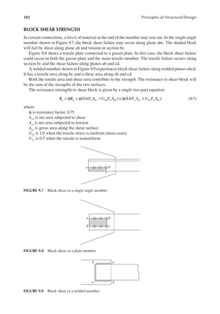
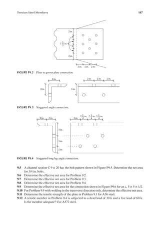
201. 183
Tension Steel Members
Example 9.4
An ∟ 6 × 4 × 1/2* tensile member of A36 steel is connected by three 7/8 in. bolts, as shown in
Figure 9.10. Determine the strength of the member.
SOLUTION
I. Tensile strength of member
A. Yielding in gross area
1. Ag = 4.75 in.2
2. h = (7/8) + (1/8) = 1 in.
3. From Equation 9.1
Pu = =
0.9(36)(4.75) 153.9k
B. Rupture in net area
1. A A
n g
( )
( )( )
= −
= − =
one hole area
4.75 1 1 1/2 4.25in.2
2. U = 0.6 for three bolts in a line
3. Ae = UAn = 0.6 (4.25) = 2.55 in.2
4. From Equation 9.2
Pu = = ←
0.75(58)(2.55) 110.9k Controls
II. Block shear strength
A. Gross shear area along ab
Agv =





 =
10
1
2
5in.2
B. Net shear area along ab
A A
nv gv
= −
= −





 =
2 holearea
5 2.5(1)
1
2
3.75in.
1
2
2
C. Net tensile area along bc
A t
nt = −
=





 −





 =
2.5 1 2 hole
2.5
1
2
1
2
(1)
1
2
1.0 in.2
D. Ubs = 1.0
E. From Equation 9.7
F A U F A
u nv bs u nt
φ + = + =
(0.6 ) 0.75[0.6(58)(3.75) (1)(58)(1.0)] 141.4 k
F A U F A
y gv bs u nt
φ + = + =
(0.6 ) 0.75[0.6(36)(5) (1)(58)(1.0)] 124.5k
The strength is 110.9 k controlled by rupture of the net section.
* Section properties not included in the appendix.
c
b
a T
2 in.
1
2
3 in.
2 in. 4 in. 4 in.
1
2
FIGURE 9.10 The three-bolt connection of Example 9.4.

202. 184 Principles of Structural Design
DESIGN PROCEDURE FOR TENSION MEMBERS
The type of connection used for a structure affects the choice of the tensile member. The bolt-type
connections are convenient for members consisting of angles, channels, and W and S shapes. The
welded connection suits plates, channels, and structural tees.
The procedure to design a tensile member consists of the following:
1. Determine the critical combination(s) of factored loads.
2. For each critical load combination, determine the gross area required by Equation 9.1 and
select a section.
3. Make provision for holes or welds based on the connection requirements, and determine
the effective net area.
4. Compute the loading capacity of the effective net area of the selected section by
Equation 9.2. This capacity should be more than the design load(s) of step 1. If it is not,
revise the selection.
5. Check the block shear strength with Equation 9.5. If it is not adequate, either revise the
connection or revise the member size.
6. The limitation of the maximum slenderness ratio of 300 is not mandatory in AISC 2010.
However, it is still a preferred practice except for rods and hangers.
Although rigid frames are common in steel structures, roof trusses having nonrigid connections are
used for industrial or mill buildings. The members in the bottom chord of a truss are commonly in
tension. Some of the web members are in tension and the others are in compression. With changing
of the wind direction, the forces in the web members alternate between tension and compression.
Accordingly, the web members have to be designed to function both as tensile as well as compression
elements.
Example 9.5
A roof system consists of a Warren-type roof truss, as shown in Figure 9.11. The trusses are spaced
25 ft. apart. The following loads are passed on to the truss through the purlins. Design the bottom
chord members consisting of the two angles section separated by a 3/8 in. gusset plate. Assume
one line of two 3/4 in. diameter bolts spaced 3 in. at each joint. Use A572 steel.
Dead load (deck, rooing, insulation) = 10 psf
Snow = 29 psf
Roof LL = 20 psf
Wind (vertical) = 16 psf
4ft.
Purlins
6 @ 6 ft.= 36
FIGURE 9.11 A Warren roof truss.

203. 185
Tension Steel Members
SOLUTION
A. Computation of loads
1. Adding 20% to dead load for the truss weight, D = 12 psf.
2. Consider the following load combinations:
a. 1.2D + 1.6(Lr or S) + 0.5W = 1.2(12) + 1.6(29) + 0.5(16) = 68.8 psf ← Controls
b. 1.2D + W + 0.5(Lr or S) = 1.2(12) + 16 + 0.5(29) = 44.9 psf
3. Tributary area of an entire truss = 36 × 25 = 900 ft.2
4. Total factored load on the truss = 68.8 × 900 = 61,920 lb or 61.92 k.
5. This load is distributed through purlins in six parts, on to ive interior joints and one-half
on each end joint since the exterior joint tributary is one-half that of the interior joints.
Thus, the joint loads are
Interior joints
61.92
6
10.32k
= =
Exterior joints
10.32
2
5.16 k
= =
B. Analysis of truss
1. The loaded truss is shown in Figure 9.12.
2. Reaction @ L0 and L6 = 61.62/2 = 30.96 k.
3. The bottom chord members L2L3 and L3L4 are subjected to the maximum force. A free-
body diagram of the left of section a-a is shown in Figure 9.13.
4. M @ U2 = 0
FL L
( ) ( ) ( )
− + + + =
30.96 12 5.16 12 10.32 6 (4) 0
2 3
F P
L L u
= ←
61.92k
2 3
30.96k 30.96k
5.16 k
4ft.
U0
10.32k
U1
10.32 k
U2
10.32 k
U3
10.32k
U4
10.32 k
U5
5.16k
U6
6 @ 6 ft.
a
a
L2
L1
L4
L3
L6
L5
L0
FIGURE 9.12 Truss analysis for Example 9.5.
5.16k
U0
10.32k
6 ft.
U1
10.32k
U2
30.96k
4 ft.
L1
6ft. L2
L3
L0
FIGURE 9.13 Free-body diagram of truss.

204. 186 Principles of Structural Design
C. Design of member
1. From Equation 9.1
A
P
F
g
u
y
= = =
0.9
61.92
0.9(50)
1.38 in.2
Try 2 ∟ 3 × 2 × 1/4 Ag = 2.4 in.2, centroid x = 0.487 (from Appendix C,
Table C.3a through c).
2. h = (3/4) + (1/8) = (7/8) in.
A A
n g
= −
= −











 =
one hole area
2.40 (1)
7
8
1
4
2.18 in.2
3. From Equation 9.6 U = − =
1
0.487
3
0.84
Ae = 0.84 (2.18) = 1.83 in.2
4. From Equation 9.2
OK
P F A
u u e
=
= = >
0.75
0.75(65)(1.83) 89.27 k 61.92 k
D. Check for block shear strength (similar to Example 9.4)
PROBLEMS
9.1 A 1/2 in. × 10 in. plate is attached to another plate by means of six 3/4 in. diameter bolts, as
shown in Figure P9.1. Determine the net area of the plate.
9.2 A 3/4 in. × 10 in. plate is connected to a gusset plate by 7/8 in. diameter bolts, as shown in
Figure P9.2. Determine the net area of the plate.
9.3 An ∟ 5 × 5 × 1/2 has staggered holes for 3/4 in. diameter bolts, as shown in Figure P9.3.
Determine the net area for the angle (Ag = 4.79 in.2, centroid x = 1.42 in.).
9.4 An ∟ 8 × 4 × 1/2 has staggered holes for 7/8 in. diameter bolts, as shown in Figure P9.4.
Determine the net area (Ag = 5.80 in.2, centroid x = 0.854 in.).
2 in. 2 in. 2 in. 2 in.
2 in.
2 in.
3 in.
3 in.
FIGURE P9.1 Plate to plate connection.

205. 187
Tension Steel Members
9.5 A channel section C 9 × 20 has the bolt pattern shown in Figure P9.5. Determine the net area
for 3/4 in. bolts.
9.6 Determine the effective net area for Problem 9.2.
9.7 Determine the effective net area for Problem 9.3.
9.8 Determine the effective net area for Problem 9.4.
9.9 Determine the effective net area for the connection shown in Figure P9.6 for an ∟ 5 × 5 × 1/2.
9.10 For Problem 9.9 with welding in the transverse direction only, determine the effective net area.
9.11 Determine the tensile strength of the plate in Problem 9.1 for A36 steel.
9.12 A tensile member in Problem 9.4 is subjected to a dead load of 30 k and a live load of 60 k.
Is the member adequate? Use A572 steel.
2 in.
2 in.
2 in. 2 in. 2 in.
1 in.
1
2
FIGURE P9.2 Plate to gusset plate connection.
3 in.
3 in. 3 in.
2 in. 2 in. 2 in.
FIGURE P9.3 Staggered angle connection.
3 in.
3 in.
2 in.
3in.
2 in. 2 in.
2 in.
1
4
2 in.
1
4
2 in.
1
4
FIGURE P9.4 Staggered long leg angle connection.

206. 188 Principles of Structural Design
9.13 Is the member in Problem 9.9 adequate to support the following loads all acting in tension?
Use A992 steel.
Dead load = 25 k
Live load = 50 k
Snow load = 40 k
Wind load = 35 k
9.14 An angle of A36 steel is connected to a gusset plate with six 3/4 in. bolts, as shown in
Figure P9.7. The member is subjected to a dead load of 25 k and a live load of 40 k. Design a
3½ in. size (3½ × ?) member.
1 in.
1
2
1 in.
1
2
in. bolts
3
4
5 spaces @ 3in.
FIGURE P9.7 Connection for Problem 9.14.
6 in.
FIGURE P9.6 Welded connection.
1 in.
3 in.
2 in. 2 in.
3 in.
1
2
1 in.
1
2
1 in.
1
2
1 in.
1
2
1 in.
1
2
1 in.
3 in.
3 in.
1
2
1 in.
1
2
FIGURE P9.5 Staggered channel connection.

207. 189
Tension Steel Members
9.15 An angle of A36 steel is connected by 7/8 in. bolts, as shown in Figure P9.8. It is exposed to
a dead load of 20 k, a live load of 45 k, and a wind load of 36 k. Design a 4 in. size (4 × ?)
member. Use A992 steel.
9.16 Compute the strength including the block shear capacity of a member comprising ∟ 3½ × 3½ ×
1/2 as shown in Figure P9.9. The bolts are 3/4 in. The steel is A36.
9.17 A tensile member comprises a W 12 × 30 section of A36 steel, as shown in Figure P9.10 with
each side of langes having three holes for 7/8 in. bolts. Determine the strength of the member
including the block shear strength.
2 in.
3 spaces @ 3in.
1 in.
1
2
1 in.
1
2
FIGURE P9.8 Two-row connection for Problem 9.15.
1 in.
1
2
1 in.
1
2
2in.
3 in.
3 in.
FIGURE P9.9 Tensile member for Problem 9.16.
1 in.
1
2
bf
2 in.
4 in.
4 in.
FIGURE P9.10 Wide lange tensile member for Problem 9.17.

208. 190 Principles of Structural Design
9.18 Determine the strength of the welded member shown in Figure P9.11, including the block
shear capacity. The steel is A572.
4 in.
Plate ×8
1
2
Plate ×10
1
2
FIGURE P9.11 Welded member for Problem 9.18.

209. 191
10 Compression Steel Members
STRENGTH OF COMPRESSION MEMBERS OR COLUMNS
The basic strength requirement or compression in the load resistance factor design format is
P P
u n
≤ φ (10.1)
where
Pu is factored axial load
ϕ = 0.9, resistance factor for compression
Pn is nominal compressive strength of the column
For a compression member that fails by yielding, Pn = Fy Ag, similar to a tensile member. However,
the steel columns are leaner; that is, the length dimension is much larger than the cross-sectional
dimension. Accordingly, the compression capacity is more often controlled by the rigidity of the
column against buckling instead of yielding. There are two common modes of failure in this respect.
1. Local instability: If the parts (elements) comprising a column are relatively very thin, a
localized buckling or wrinkling of one or more of these elements may occur prior to the
instability of the entire column. Based on the ratio of width to thickness of the element, a
section is classiied as a slender or a nonslender for the purpose of local instability.
2. Overall instability: Instead of an individual element getting winkled, the entire column
may bend or buckle lengthwise under the action of the axial compression force. This can
occur in three different ways.
a. Flexural buckling: A delection occurs by bending about the weak axis, as shown in
Figure 10.1. The slenderness ratio is a measure of the lexural buckling of a member.
When the buckling occurs at a stress level within the proportionality limit of steel, it is
called elastic buckling. When the stress at buckling is beyond the proportionality limit,
it is inelastic buckling. The columns of any shape can fail in this mode by either elastic
or inelastic buckling.
b. Torsional buckling: This type of failure is caused by the twisting of the member lon-
gitudinally, as shown in Figure 10.2. The doubly symmetric hot-rolled shapes like
W, H, or round are normally not susceptible to this mode of buckling. The torsional
buckling of doubly symmetric sections can occur only when the torsional unbraced
length exceeds the lateral lexural unbraced length. The thinly built-up sections might
be exposed to torsional buckling.
c. Flexural–torsional buckling: This failure occurs by the combination of lexural and
torsional buckling when a member twists while bending, as shown in Figure 10.3. Only
the sections with a single axis of symmetry or the nonsymmetric sections such as a
channel, tee, and angle are subjected to this mode of buckling.
The nominal compressive strength, Pn, in Equation 10.1 is the lowest value obtained according to
the limit states of lexural buckling, torsional buckling, and lexural-torsional buckling.
The lexural buckling limit state is applicable to all sections.
In addition, the doubly symmetric sections having torsional unbraced length larger than the weak-
axis lexural unbraced length, the doubly symmetric sections built from thin plates, singly symmet-
ric sections, and nonsymmetric sections are subjected to torsional buckling or lexural-torsional

210. 192 Principles of Structural Design
FIGURE 10.1 Flexural buckling.
FIGURE 10.2 Torsional buckling.
FIGURE 10.3 Flexural–torsional buckling.

211. 193
Compression Steel Members
buckling that requires substantive evaluations. It is desirable to prevent it when feasible. This can be
done by bracing the member to prevent twisting.
The limit states are considered separately for the nonslender and the slender sections according
to the local instability criteria.
LOCAL BUCKLING CRITERIA
In the context of local buckling, the elements of a structural section are classiied into following two
categories:
1. Unstiffened element: This has an unsupported edge (end) parallel to (along) the direction
of the load, like an angle section.
2. Stiffened element: This is supported along both of its edges, like the web of a wide lange section.
The two types of elements are illustrated in Figure 10.4.
When the ratio of width to thickness of an element of a section is greater than the speciied limit
λr, as shown in Table 10.1, it is classiied as a slender shape. The cross section of a slender element
is not fully effective in resisting a compressive force. Such elements should be avoided or else their
U
t U U
U
U
U U
U U
S
S
S
S
S S
S
d d
h
h D
U= Unstiffened
S = Stiffened
h
tf
t
tw
tw
tw
tw
tf
tf
tf
bf bf
b
b
b
U
U
FIGURE 10.4 Stiffened and unstiffened elements.
TABLE 10.1
Slenderness Limit for Compression Member
Element
Width :
Thickness Ratio λr Magnitude for 36 ksi Magnitude for 50 ksi
W, S, M, H bf/2tf 0.56 E Fy 15.89 13.49
h/tw 1.49 E Fy 42.29 35.88
C bf/tf 0.56 E Fy 15.89 13.49
h/tw 1.49 E Fy 42.29 35.88
T bf/2tf 0.56 E Fy 15.89 13.49
d/tw 0.75 E Fy 21.29 18.16
Single ∟ or double
∟ with separation
b/t 0.45 E Fy 12.77 10.84
Box, tubing b/t 1.4 E Fy Box (46 ksi steel) 35.15 Tubing (42 ksi steel) 36.79
Circular D/t 0.11(E/Fy) Pipe (35 ksi steel) 91.14

212. 194 Principles of Structural Design
strength should be reduced, as discussed in the “Slender Compression Members” section. Separate
provisions for strength reduction are made in the AISC manual for stiffened and unstiffened
sections. The terms are explained in Figure 10.4.
FLEXURAL BUCKLING CRITERIA
The term (KL/r), known as the slenderness ratio, is important in column design. Not only does
the compression capacity of a column depend on the slenderness ratio, but the ratio also sets
a limit between the elastic and nonelastic buckling of the column. When the slenderness ratio
exceeds a value of 4.71 /
E Fy , the column acts as an elastic column and the limiting (failure)
stress level is within the elastic range.
According to the classic Euler formula, the critical load is inversely proportional to (KL/r)2, where
K is the effective length factor (coeficient), discussed in the “Effective Length Factor for Slenderness
Ratio” section, L is the length of the column, and r is the radius of gyration given by I A
/ .
Although it is not a mandatory requirement in the AISC Manual 2010, the AISC recommends
that the slenderness ratio for a column should not exceed a value of 200.
EFFECTIVE LENGTH FACTOR FOR SLENDERNESS RATIO
The original lexural buckling or Euler formulation considered the column pinned at both ends.
The term K was introduced to account for the other end conditions because the end condition will
make a column buckle differently. For example, if a column is ixed at both ends, it will buckle at
the points of inlection about L/4 distance away from the ends, with an effective length of one-half
of the column length. Thus, the effective length of a column is the distance at which the column is
assumed to buckle in the shape of an elastic curve. The length between the supports, L, is multiplied
by a factor to calculate the effective length.
When columns are part of a frame, they are constrained at the ends by their connection to beams
and to other columns. The effective length factor for such columns is evaluated by the use of the
alignment charts or nomographs given in Figures 10.5 and 10.6; the former is for the braced frames
where the sidesway is prevented, and the latter is for the moment frames where the sidesway is
permitted.
In the nomographs, the subscripts A and B refer to two ends of a column for which K is desired.
The term G is the ratio of the column stiffness to the girder stiffness expressed as
/
/
G
I L
I L
c c
g g
∑
∑
= (10.2)
where
Ic is moment of inertia of the column section
Lc is length of the column
Ig is moment of inertia of the girder beam meeting the column
Lg is length of the girder
∑ is summation of all members meeting at joint A for GA and at joint B for GB
The values of Ic and Ig are taken about the axis of bending of the frame. For a column base con-
nected to the footing by a hinge, G is taken as 10 and when the column is connected rigidly (ixed)
to the base, G is taken as 1.
After determining GA and GB for a column, K is obtained by connecting a straight line between
points GA and GB on the nomograph. Since the values of I (moment of inertia) of the columns and

213. 195
Compression Steel Members
50.0
GB
K
50.0
10.0 10.0
5.0 5.0
4.0 4.0
3.0 3.0
2.0 2.0
1.0 1.0
1.0
0.9 0.9
0.9
0.8 0.8
0.8
0.7 0.7
0.7
0.6 0.6
0.6
0.5 0.5
0.5
0.4 0.4
0.3 0.3
0.2 0.2
0.1 0.1
0.0 0.0
GA
∞ ∞
FIGURE 10.5 Alignment chart, sidesway prevented. (Courtesy of American Institute of Steel Construction,
Chicago, IL.)
100.0
∞
GA K
50.0
30.0
20.0
10.0
8.0
7.0
6.0
5.0
4.0
3.0
2.0
1.0
0.0
100.0
∞
GB
50.0
30.0
20.0
10.0
8.0
7.0
6.0
5.0
4.0
3.0
2.0
1.0
0.0
20.0
∞
10.0
5.0
4.0
3.0
2.0
1.5
1.0
FIGURE 10.6 Alignmentchart,sideswaynotprevented.(CourtesyofAmericanInstituteofSteelConstruction,
Chicago, IL.)

214. 196 Principles of Structural Design
beams at the joint are required to determine G, the factor K cannot be determined unless the size of
the columns and the beams are known. On the other hand, the factor K is required to determine the
column size. Thus, these nomographs need some preliminary assessments of the value of K and the
dimensions of the columns and girders.
One of the conditions for the use of the nomographs or the alignment charts is that all columns
should buckle elastically, that is, 4.71 /
KL E Fy
> . If a column buckles inelastically, a stiffness
reduction factor, τa, has to be applied. The factor τa is the ratio of the tangent modulus of elasticity
to the modulus of elasticity of steel. The value has been tabulated in the AISC manual as a function
of Pu/Ag. Without τa, the value of K is on the conservative side.
However, in lieu of applying the monographs in a simpliied method, the factors (coeficients)
listed in Figure 7.6 are used to ascertain the effective length. Figure 7.6 is used for isolated columns
also. When Figure 7.6 is used for the unbraced frame columns, the lowest story (base) columns
could be approximated by the condition with K = 2 for the hinged base and K = 1.2 for the ixed
base, and the upper story columns are approximated by the condition with K = 1.2. For braced
frames, the condition with K = 0.65 is a good approximation.
Example 10.1
A rigid unbraced moment frame is shown in Figure 10.7. Determine the effective length factors
with respect to weak axis for members AB and BC.
SOLUTION
1. The section properties and G ratios are arranged in the table below:
C
B
A
W14×22 W14×26
W10
×
26
W10
×
33
W12×14
W12×14
12 ft.
15 ft.
20 ft. 20 ft.
FIGURE 10.7 An unbraced frame.
Joint
Column Girder
Section i (in.4) L (ft.) i/L Section i (in.4) L (ft.) i/L G
A Fixed 1
B W10 × 33 171 15 11.40a
W14 × 22 199 20 9.95
W10 × 26 144 12 12.00 W14 × 26 245 20 12.25
∑ 23.40 22.20 23.4/22.20 = 1.05
C W10 × 26 144 12 12.00 W12 × 14 88.6 20 4.43
W12 × 14 88.6 20 4.43
∑ 12.00 8.86 12.00/8.86 = 1.35
a Mixed units (I in in.4 and L in ft.) can be used since the ratio is being used.

215. 197
Compression Steel Members
2. Column AB
From Figure 10.6, the alignment chart for an unbraced frame (sidesway permitted) connect-
ing a line from GA = 1 to GB = 1.05, K = 1.3.
3. Column BC
From the alignment chart with GA = 1.05 (point B) and GB = 1.35 (point C), K = 1.38.
LIMIT STATES FOR COMPRESSION DESIGN
The limit states of design of a compression member depends on the category to which the compres-
sion member belongs, as described in the “Strength of Compression Members or Columns” section.
The limit states applicable to different categories of columns are summarized in Table 10.2.
AISC 360-10 has organized the provisions for compression members as follows:
1. Flexural buckling of nonslender members
2. Torsional buckling and lexural-torsional buckling of nonslender members
3. Single-angle members
4. Built-up members by combining two shapes
5. Slender members
The discussion below follows the same order.
NONSLENDER MEMBERS
FLEXURAL BUCKLING OF NONSLENDER MEMBERS IN ELASTIC AND INELASTIC REGIONS
Based on the limit state for lexural buckling, the nominal compressive strength Pn is given by
P F A
n cr g
= (10.3)
TABLE 10.2
Applicable Limit States for Compressive Strength
Local Buckling (Local Instability)
Type of Column Nonslender Column, λ ≤ λr Slender Column, λ > λr
Overall Instability
1. Doubly symmetric members Flexural buckling in elastic or inelastic
region
Flexural buckling in elastic or
inelastic region incorporating the
reduction factors for slender element
2. Doubly symmetric thin plate
builtup members or large
unbraced torsional length
members
Lowest of the following two limits:
1. Flexural buckling in elastic or
inelastic region
2. Torsional buckling
Lowest of the following two limits,
incorporating the reduction factors
for slender element:
1. Flexural buckling in elastic or
inelastic region
2. Torsional buckling
3. Singly symmetric or
nonsymmetric members
Lowest of the following three limits:
1. Flexural buckling in elastic or
inelastic region
2. Flexural–torsional buckling
Lowest of the following three limits,
incorporating the reduction factors
for slender element:
1. Flexural buckling in elastic or
inelastic region
2. Flexural–torsional buckling

216. 198 Principles of Structural Design
where
Fcr is lexural buckling state (stress)
Ag is gross cross-sectional area
Including the nominal strength in Equation 10.1, the strength requirement of a column can be
expressed as
P F A
u cr g
= φ (10.4)
The lexural buckling stress, Fcr is determined as follows.
INELASTIC BUCKLING
When / 4.71 / ,
KL r E Fy
≤ we have inelastic buckling, for which
(0.658 )
/
F F
cr
F F
y
y e
= (10.5)
where Fe is elastic critical buckling or Euler stress calculated according to Equation 10.6:
( / )
2
2
F
E
KL r
e =
π
(10.6)
ELASTIC BUCKLING
When / 4.71 /
KL r E Fy
> , we have elastic buckling, for which
0.877
F F
cr e
= (10.7)
The value of 4.71 /
E Fy , at the threshold of inelastic and elastic buckling, is given in Table 10.3
for various types of steel.
The available critical stress ϕFcr in Equation 10.4 for both the inelastic and elastic regions is
given in Table 10.4 in terms of KL/r, adapted from the AISC Manual 2010.
TORSIONAL AND FLEXURAL–TORSIONAL BUCKLING OF NONSLENDER MEMBERS
According to the commentary in Section E of AISC 360-10, in the design with hot-rolled column
sections, the torsional buckling of symmetric shapes and the lexural-torsional buckling of nonsym-
metric shapes are the failure modes that are not usually considered in design. They usually do not
govern or the critical load differs very little from the lexural buckling mode.
Hence, this section usually applies to double-angle, tee-shaped, and other built-up members.
TABLE 10.3
Numerical Limits of
Inelastic–Elastic Buckling
Type of Steel 4.71 e/Fy
A36 133.7
A992 113.43
A572 113.43

217. 199
Compression Steel Members
TABLE 10.4
Available Critical Stress ϕFcr for Compression Members (Fy = 50 ksi and ϕ = 0.90)
KL/r ϕFcr, ksi KL/r ϕFcr, ksi KL/r ϕFcr, ksi KL/r ϕFcr, ksi KL/r ϕFcr, ksi
1 45.0 41 39.8 81 27.9 121 15.4 161 8.72
2 45.0 42 39.5 82 27.5 122 15.2 162 8.61
3 45.0 43 39.3 83 27.2 123 14.9 163 8.50
4 44.9 44 39.1 84 26.9 124 14.7 164 8.40
5 44.9 45 38.8 85 26.5 125 14.5 165 8.30
6 44.9 46 38.5 86 26.2 126 14.2 166 8.20
7 44.8 47 38.3 87 25.9 127 14.0 167 8.10
8 44.8 48 38.0 88 25.5 128 13.8 168 8.00
9 44.7 49 37.7 89 25.2 129 13.6 169 7.89
10 44.7 50 37.5 90 24.9 130 13.4 170 7.82
11 44.6 51 37.2 91 24.6 131 13.2 171 7.73
12 44.5 52 36.9 92 24.2 132 13.0 172 7.64
13 44.4 53 36.7 93 23.9 133 12.8 173 7.55
14 44.4 54 36.4 94 23.6 134 12.6 174 7.46
15 44.3 55 36.1 95 23.3 135 12.4 175 7.38
16 44.2 56 35.8 96 22.9 136 12.2 176 7.29
17 44.1 57 35.5 97 22.6 137 12.0 177 7.21
18 43.9 58 35.2 98 22.3 138 11.9 178 7.13
19 43.8 59 34.9 99 22.0 139 11.7 179 7.05
20 43.7 60 34.6 100 21.7 140 11.5 180 6.97
21 43.6 61 34.3 101 21.3 141 11.4 181 6.90
22 43.4 62 34.0 102 21.0 142 11.2 182 6.82
23 43.3 63 33.7 103 20.7 143 11.0 183 6.75
24 43.1 64 33.4 104 20.4 144 10.9 184 6.67
25 43.0 65 33.0 105 20.1 145 10.7 185 6.60
26 42.8 66 32.7 106 19.8 146 10.6 186 6.53
27 42.7 67 32.4 107 19.5 147 10.5 187 6.46
28 42.5 68 32.1 108 19.2 148 10.3 188 6.39
29 42.3 69 31.8 109 18.9 149 10.2 189 6.32
30 42.1 70 31.4 110 18.6 150 10.0 190 6.26
31 41.9 71 31.1 111 18.3 151 9.91 191 6.19
32 41.8 72 30.8 112 18.0 152 9.78 192 6.13
33 41.6 73 30.5 113 17.7 153 9.65 193 6.06
34 41.4 74 30.2 114 17.4 154 9.53 194 6.00
35 41.2 75 29.8 115 17.1 155 9.40 195 5.94
36 40.9 76 29.5 116 16.8 156 9.28 196 5.88
37 40.7 77 29.2 117 16.5 157 9.17 197 5.82
38 40.5 78 28.8 118 16.2 158 9.05 198 5.76
39 40.3 79 28.5 119 16.0 159 8.94 199 5.70
40 40.0 80 28.2 120 15.7 160 8.82 200 5.65
Source: Courtesy of American Institute of Steel Construction, Chicago, Illinois.

218. 200 Principles of Structural Design
The nominal strength is governed by Equation 10.3. Also, the Fcr value is determined according to
Equation 10.5 or 10.7 except for two-angle and tee-shaped members. For two-angle and tee-shaped
section, Fcr is determined directly by a different type of equation. For simplicity, Equation 10.5 or
10.7 can be used with y axis strength.
However, to determine the Euler stress Fe, instead of Equation 10.6, a different set of formulas is
used that includes the warping and torsional constants for the section.
SINGLE-ANGLE MEMBERS
For single angles with b/t ≤ 20, only the lexural limit state is to be considered. This applies to
all currently produced hot-rolled angles. Thus, the lexural–torsional limit state applies only to
fabricated angles with b/t > 20, for which the provisions of the “Torsional and Flexural–Torsional
Buckling of Nonslender Members” section apply.
AISC provides a simpliied approach in which load is applied through one connected leg. The
slenderness ratio is computed by a speciied equation. Then, Equations 10.4 through 10.7 are used
to determine the capacity.
BUILT-UP MEMBERS
The members are made by interconnecting elements by bolts or welding. The empirical relations
for the effective slenderness ratio for the composite section is used to consider the built-up member
acting as a single unit. Depending on the shape of the section, it is designed according to the lexural
buckling or lexural-torsional buckling.
SLENDER COMPRESSION MEMBERS
The approach to design slender members having λ > λr is similar to the nonslender members in all
categories except that a slenderness reduction factor, Q, is included in the expression 4.7 /
E Fy to
classify the inelastic and elastic regions and Q is also included in the equations for Fcr. The slender-
ness reduction factor Q has two components: Qs for the slender unstiffened elements and Qa for the
slender stiffened elements. These are given by a set of formulas for different shapes of columns.
A reference is made to the Section E7 of Chapter 16 of the AISC manual 2010.
All W shapes have nonslender langes for A992 steel. All W shapes listed for the columns in the
AISC manual have nonslender webs (except for W14 × 43). However, many W shapes meant to be
used as beams have slender webs in the compression.
This chapter considers only the doubly symmetric nonslender members covered in the “Nonslender
Members” section. By proper selection of a section, this condition, that is, λ ≤ λr could be satisied.
USE OF THE COMPRESSION TABLES
Section 4 of the AISC Manual 2010 contains tables concerning “available strength in axial compression,
in kips” for various shapes and sizes. These tables directly give the capacity as a function of effective
length (KL) with respect to least radius of gyration for various sections. The design of columns is a
direct procedure from these tables. An abridged table for Fy = 50 ksi is given in Appendix C, Table C.8.
When the values of K and/or L are different in the two directions, both KxLx and KyLy are
computed. If KxLx is bigger, it is adjusted as KxLx/(rx/ry). The higher of the adjusted KxLx/(rx/ry) and
KyLy value is entered in the table to pick a section that matches the factored design load Pu.
When designing for a case when KxLx is bigger, the adjustment of KxLx/(rx/ry) is not straightfor-
ward because the values of rx and ry are not known. The initial selection could be made based on the
KyLy value and then the adjusted value of KxLx/(rx/ry) is determined based on the initially selected
section.

219. 201
Compression Steel Members
Example 10.2
A 25-ft.- long column has one end rigidly ixed to the foundation. The other end is braced (ixed)
in the weak axis and free to translate in the strong axis. It is subjected to a dead load of 120 k and
a live load of 220 k. Design the column using A992 steel.
SOLUTION
A. Analytical solution
1. Assume a dead load of 100 lbs/ft.
Weight of column = 25(0.1) = 2.5 k
2. Factored design load
Pu = 1.2(120 + 2.5) + 1.6(220) = 499 k
3. For yield limit state
A
P
F
g
u
y
=
φ
= =
499
0.9(50)
11.1 in.2
4. The size will be much larger than step 3 to allow for the buckling mode of failure
r
r
b
t
h
t
E
F
E
F
x
y
f
f
w
y
y
× =
=
=
=
=
= =
= =
Select a section W14 61A 17.9 in.
5.98 in.
2.45 in.
2
7.75
30.4
0.56 0.56
29,000
50
13.49
1.49 1.49
29,000
50
35.88
2
5. Since b t E F h t E F
f f y w y
< <
/2 0.56 / and / 1.49 / , it is a nonslender section
6.
OK
K
K
K L
r
K L
r
x
y
x x
x
y x
y
=
=
=
×
=
=
×
= ←
<
1.2 from Figure 7.6
0.65
1.2(25 12)
5.98
60.2
0.65(25 12)
2.45
79.59 Controls
Since 79.59 200
7. From Table 10.3, E Fy =
4.71 / 113.43
Since 79.59 < 113.43, inelastic buckling
8. F
E
KL r
e =
π
=
π
=
( / )
(29,000)
(79.59)
45.14 ksi
2
2
2
2
9. Fcr = (0.65850/45.14)50 = 31.45 ksi
10. ϕPn = (0.9)(31.45)(17.9) = 507 k OK
B. Use of Appendix C, Table C.8
1. K L
K L
x x
y y
1.2(25) 30 ft.
0.65(25) 16.25 ft.
= =
= =
2. Select preliminary section
Based on KyLy = 16.25 ft., section W14 × 61, capacity = 507 k (interpolated), from
Appendix C, Table C.8

220. 202 Principles of Structural Design
3. For section W14 × 61, rx = 5.98 in., ry = 2.45 in.
K L
r r
x x
x y
Adjusted
/
1.2(25)
5.98/2.45
12.29
= =
Use the larger value of KyLy of 16.25 ft.
4. Section from Appendix C, Table C.8 W14 × 61 with capacity = 507 k
Example 10.3
An unbraced hinged at base column as shown in Figure 10.8 is fabricated from Grade 50 steel.
Determine the limit state that will control the design of the column.
SOLUTION
1. The doubly symmetric built-up section will be subjected to lexural-torsional buckling.
2.
b
t
E
Fy
= =
= =
10
0.25
40
1.4 1.4
29,000
50
33.72
Since 40 > 33.72, it is a slender column; the reduction factors have to be applied.
3.
1
12
(10)(10)
1
12
(9.5)(9.5)
154.58 in.
(10)(10) (9.5)(9.5)
9.75in.
154.58
9.75
3.98 in.
out inside
3 3
4
2
I I I
A
r
I
A
= −
= −
=
= −
=
= = =
4.
K
KL
r
E
F
KL
r
E
F
y
y
2.0
2.0(20 12)
3.98
120.6
From Table 10.2,4.71 113.43
4.71 , elastic flexural buckling
=
=
×
=
=
>
5. The lowest of the following two limit states will control:
a. Elastic lexural buckling with the slender reduction factors
b. Torsional buckling with the slender reduction factors
10 in.
10 in.
20 ft.
0.25in.
FIGURE 10.8 Built-up column.

221. 203
Compression Steel Members
PROBLEMS
10.1 A W8 × 31 column of A36 steel is 20 ft. long. Along the y axis, it is hinged at both ends.
Along the x axis, it is hinged at one end and free to translate at the other end. In which
direction is it likely to buckle? (rx = 3.47 in., ry = 2.02 in.)
10.2 An HSS 5 × 21
2 × 1/4 braced column is supported, as shown in Figure P10.1. Determine
the controlling (higher) slenderness ratio.
10.3 A single-story single-bay frame has the relative I values shown in Figure P10.2. Determine
the effective length of the columns along the x axis. Sway is permitted in x direction.
10.4 The frame of Figure P10.3 is braced and bends about the x axis. All beams are W18 × 35,
and all columns are W10 × 54. Determine the effective length factors for AB and BC.
10.5 An unbraced frame of Figure P10.4 bends along the x axis. Determine the effective length
factors for AB and BC.
10.6 Determine the effective length factors for AB and BC of the frame of Figure P10.4 for
bending along the y axis. Whether the factors determined in Problem 10.5 or the factors
determined in Problem 10.6 will control the design?
20 ft.
Strong axis Weak axis
10 ft.
10 ft.
Hinged
FIGURE P10.1 An HSS column.
3I
I I 15 ft.
40 ft.
FIGURE P10.2 Frame for Problem 10.3.
C
B
A
12 ft.
15 ft.
20 ft. 20 ft.
FIGURE P10.3 Frame for Problem 10.4.

222. 204 Principles of Structural Design
10.7 Determine the strength of the column of A992 steel in Figure P10.5, when (a) the length is
15 ft. and (b) the length is 30 ft.
10.8 Compute the strength of the member of A36 steel shown in Figure P10.6.
10.9 Compute the strength of the member (translation permitted) shown in Figure P10.7 of
A500 Grade B steel.
10.10 A W18 × 130 section is used as a column with one end pinned and the other end ixed
against rotation but is free to translate. The length is 12 ft. Determine the strength of the
A992 steel column.
10.11 Determine the maximum dead and live loads that can be supported by the compression
member shown in Figure P10.8. The live load is twice the dead load.
W14× 30
W14×34
W14
×
30
W14×30
W10
×
45
W16× 36 W16×36
W18
×
35
A
B
C
D
25 ft. 20 ft.
14 ft.
15 ft.
18 ft.
FIGURE P10.4 Frame for Problem 10.5.
W12 ×72
FIGURE P10.5 Column for Problem 10.7.
HP12 × 84
A= 24.6 in.2
d= 12.28 in.
rx = 5.14 in.
ry =2.94 in.
16 ft.
= 8.97
bf
2tf
= 14.2
h
tw
FIGURE P10.6 Column for Problem 10.8.

223. 205
Compression Steel Members
10.12 Determine the maximum dead and live loads supported by the braced column of Figure
P10.9. The live load is one-and-a-half times the dead load.
10.13 Determine whether the braced member of A992 steel in Figure P10.10 is adequate to sup-
port the loads as indicated.
10.14 Check whether the A36 steel member of Figure P10.11 unbraced at the top is adequate for
the indicated loads.
10.15 An HSS 6 × 4 × 5/16 braced section (46 ksi steel) shown in Figure P10.12 is applied by a
dead load of 40 k and a live load of 50 k. Check the column adequacy.
HSS 10 ×6 ×
A =24.6 in.2
rx = 3.6 in.
ry = 2.39 in.
15 ft.
A500 Grade B = 9.90
b
t
= 18.5
h
t
1
2
FIGURE P10.7 Column for Problem 10.9.
W12×79
A992 steel
12 ft.
FIGURE P10.8 Column for Problem 10.11.
20 ft. HSS 8×4×
A500 Grade B steel
1
4
A = 5.24 in.2
rx= 2.85 in.
ry= 1.66 in.
b
t
=14.2
h
t
=31.3
FIGURE P10.9 Column for Problem 10.12.
25 ft.
W12 ×72
A992 steel
D = 100 k
L = 250k
FIGURE P10.10 Column for Problem 10.13.

224. 206 Principles of Structural Design
10.16 Select an HSS section for the braced column shown in Figure P10.13.
10.17 Design a standard pipe section of A53 Grade B steel for the braced column shown in
Figure P10.14.
10.18 Select a W14 shape of A992 steel for the braced column of 25 ft. length shown in
Figure P10.15. Both ends are ixed. There are bracings at 10 ft. from top and bottom in the
weaker direction.
10.19 Design a W14 section column AB of the frame shown in Figure P10.16. It is unbraced along
the x axis and braced in the weak direction. The loads on the column are dead load = 200 k
and live load = 600 k. First determine the effective length factor using Figure 7.6. After
selecting the preliminary section for column AB, use the alignment chart with the same
size for column BC as of column AB to revise the selection. Use W16 × 100 for the beam
sections meeting at B.
15 ft.
x axis y axis
D= 100 k
L= 250 k
6 ft.
9 ft.
HP 10×57 A = 16.7 in.2
rx=4.18 in.
ry=2.45 in.
bf
2tf
= 9.03
h
tw
= 13.9
FIGURE P10.11 Column for Problem 10.14.
15 ft.
D= 40 k
L= 50 k
7 ft.
8 ft.
HSS 6×4× 5
16
FIGURE P10.12 Column for Problem 10.15.
D = 50 k
L = 100 k
12 ft.
FIGURE P10.13 Column for Problem 10.16.

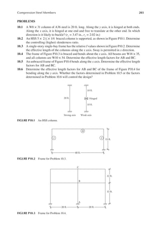
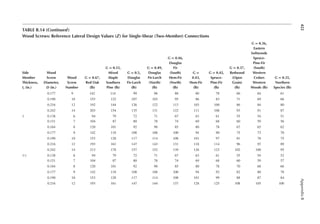
225. 207
Compression Steel Members
10.20 Design the column AB in Problem 10.19 for the frame braced in both directions.
10.21 A WT12 × 34 column of 18 ft. length is pinned at both ends. Show what limiting states
will determine the strength of the column. Use A992 steel. [A = 10 in.2, ry = 1.87 in.,
bf/2tf = 7.66, d/tw = 28.7]
10.22 The A572 braced steel column in Figure P10.17 is ixed at one end and hinged at the other
end. Indicate the limit states that will control the strength of the column.
10.23 A double-angle braced section with a separation 3/8 in. is subjected to the loads shown in
Figure P10.18. Determine the limit states that will govern the design of the column. Use
Grade 50 steel. [A = 3.86 in.2, ry = 1.78 in., b/t = 16]
12 ft.
D =50 k
L= 100 k
FIGURE P10.14 Column for Problem 10.17.
25 ft.
x axis y axis
D =350 k
L= 1000k
10 ft.
10 ft.
5 ft.
FIGURE P10.15 Column for Problem 10.18.
D 100 k
L 300 k
200 k
600 k
C
B
A
100 k
300 k
12 ft.
12 ft.
12 ft.
20 ft.
20 ft.
FIGURE P10.16 Frame for Problem 10.19.

226. 208 Principles of Structural Design
10.24 A cruciform column is fabricated from Grade 50 steel, as shown in Figure P10.19.
Determine the limit states that will control the design. [Use the properties of a single
angle to determine the values of the composite section.]
10.25 For the braced column section and the loading shown in Figure P10.20, determine the
limit states for which the column should be designed. Use A992 steel.
12 ft. C12 ×30
FIGURE P10.17 Column for Problem 10.22.
16 ft.
D =50 k
L =100 k
2 4 ×4 ×
4
1
A = 3.86 in.2
ry= 1.78 in.
b
t
= 16
FIGURE P10.18 Column for Problem 10.23.
25 ft.
1 ×20 plate
1 ×18 plate
1 ×20 plate
Strong axis Weak axis
D= 200 k
L= 500 k
12 ft.
13 ft.
FIGURE P10.20 Built-up column for Problem 10.25.
15 ft.
4 3 ×3 ×
4
1
2
1
2
1
FIGURE P10.19 Cruciform column for Problem 10.24.

227. 209
11 Flexural Steel Members
BASIS OF DESIGN
Beams are the structural members that support transverse loads on them and are subjected to lexure
and shear. An I shape is a common cross section for a steel beam where the material in the langes at
the top and bottom is most effective in resisting bending moment and the web provides for most of
the shear resistance. As discussed in the “Design of Beams” section of Chapter 7— context of wood
beams—the design process involves selection of a beam section on the basis of the maximum bend-
ing moment to be resisted. The selection is, then, checked for shear capacity. In addition, the service-
ability requirement imposes the delection criteria for which the selected section should be checked.
The basis of design for bending or lexure is as follows:
≤ φ
M M
u n (11.1)
where
Mu is factored design (imposed) moment
ϕ is resistance factor for bending = 0.9
Mn is nominal moment strength of steel
NOMINAL STRENGTH OF STEEL IN FLEXURE
Steel is a ductile material. As discussed in the “Elastic and Plastic Designs” section in Chapter 1,
steel can acquire the plastic moment capacity Mp, wherein the stress distribution above and below
the neutral axis will be represented by the rectangular blocks corresponding to the yield strength of
steel, that is, Mp = FyZ, Z being the plastic moment of inertia of the section.
However, there are certain other factors that undermine the plastic moment capacity. One such fac-
tor relates to the unsupported (unbraced) length of the beam, and another relates to the slender dimen-
sions of the beam section. The design capacity is determined considering both of these. The effect
of the unsupported length on strength is discussed irst in the “Lateral Unsupported Length” section.
The beam’s slender dimensions affect the strength similar to the local instability of compression
members. This is described in the “Noncompact and Slender Beam Sections for Flexure” section.
LATERAL UNSUPPORTED LENGTH
As a beam bends, it develops compression stress in one part and tensile stress in the other part of its
cross section. The compression region acts analogous to a column. If the entire member is slender, it
will buckle outward similar to a column. However, in this case the compression portion is restrained
by the tensile portion. As a result, a twist will occur in the section. This form of instability, as shown
in Figure 11.1, is called lateral torsional buckling.
Lateral torsional buckling can be prevented in two ways:
1. Lateral bracings can be applied to the compression lange at close intervals, which prevents
the lateral translation (buckling) of the beam, as shown in Figure 11.2. This support can be
provided by a loor member securely attached to the beam.
2. Cross bracings or a diaphragm can be provided between adjacent beams, as shown in
Figure 11.3, which directly prevents the twisting of the sections.

228. 210 Principles of Structural Design
Depending on the lateral support condition on the compression side, the strength of the limit
state of a beam is due to either the plastic yielding of the section or the lateral torsional buckling of
the section. The latter condition has two further divisions: inelastic lateral torsional buckling and
elastic lateral torsional buckling. These three zones of the limit states are shown in Figure 11.4 and
described here.
In Figure 11.4, the irst threshold value for the unsupported or the unbraced length is Lp, given
by the following relation:
= 1.76
L r
E
F
p y
y
(11.2)
where
Lp is irst threshold limit for the unsupported length (in inches)
ry is radius of gyration about the y axis, listed in the Appendix C, Tables C.1 through C.7
The second threshold value is Lr, which is conservatively given by the following relation:
= π
0.7
L r
E
F
r ts
y
(11.3)
FIGURE 11.2 Lateral bracing of compression lange.
FIGURE 11.3 Cross bracing or diaphragm.
0.7
Nominal
moment,
M
n
Unbraced length, Lb
Adequate
lateral
support
Partial
adequate
lateral support
Inadequate
lateral support
Elastic
lateral torsional
buckling
Inelastic
lateral torsional
buckling
Mp
Lp Lr
Fy
FIGURE 11.4 Nominal moment strength as a function of unbraced length.
FIGURE 11.1 Buckling and twisting effect in a beam.

229. 211
Flexural Steel Members
where
Lr is second threshold of the unsupported length (in inches)
rts is special radius of gyration for Lr, listed in Appendix C, Tables C.1 through C.7
FULLY PLASTIC ZONE WITH ADEQUATE LATERAL SUPPORT
When the lateral support is continuous or closely spaced so that the unbraced (unsupported) length
of a beam, Lb, is less than or equal to Lp from Equation 11.2, the beam can be loaded to reach the
plastic moment capacity throughout the section.
The limit state in this case is the yield strength given as follows:
= φ φ =
, with 0.9
M F Z
u y x (11.4)
The lateral torsional buckling does not apply in this zone.
INELASTIC LATERAL TORSIONAL BUCKLING ZONE
When the lateral unsupported (unbraced) length, Lb, is more than Lp but less than or equal to Lr, the
section will not have suficient capacity to develop the plastic moment capacity, i.e., the full yield
stress, Fy, in the entire section. Before all ibers are stressed to Fy buckling will occur. This will lead
to inelastic lateral torsional buckling.
At Lb = Lp, the moment capacity is the plastic capacity Mp. As the length Lb increases beyond
the Lp value, the moment capacity becomes less. At the Lr value of the unbraced length, the section
buckles elastically, attaining the yield stress only at the top or the bottom iber. Accounting for the
residual stress in the section during manufacturing, the effective yield stress is Fy − Fr, where Fr is
residual stress. The residual stress is taken as 30% of the yield stress. Thus, at Lb = Lr the moment
capacity is (Fy – Fr)Sx or 0.7FyS.
When the unbraced length Lb is between the Lp and Lr values, the moment capacity is linearly
interpolated between the magnitudes of Mp and 0.7FyS as follows:
= φ
−
−














– ( – 0.7 )
M M M F S
L L
L L
C
u p p y
b p
r p
b (11.5)
where Mp = FyZx
MODIFICATION FACTOR cb
The factor Cb is introduced in Equation 11.5 to account for a situation when the moment within the
unbraced length is not uniform (constant). A higher moment between the supports increases the resis-
tance to torsional buckling, thus resulting in an increased value of Cb. This factor has the following
values:
A value of 1 is conservatively taken.
cb
1. No transverse loading between brace points 1
2. Uniformly loaded simple supported beam 1.14
3. Centrally loaded simple supported beam 1.32
4. Cantilever beam 1
5. Equal end moments of opposite signs 1
6. Equal end moments of the same sign (reverse curvature) 2.27
7. One end moment is 0 1.67

230. 212 Principles of Structural Design
ELASTIC LATERAL TORSIONAL BUCKLING ZONE
When the unbraced length Lb exceeds the threshold value of Lr, the beam buckles before the effective
yield stress, 0.7Fy, is reached anywhere in the cross section. This is elastic buckling. The moment
capacity is made up of the torsional resistance and the warping resistance of the section:
< φ
0.7
M F S
u y (11.6)
At Lb = Lr, the capacity Mu is exactly 0.7ϕFyS.
NONCOMPACT AND SLENDER BEAM SECTIONS FOR FLEXURE
The aforementioned discussion on beam strength did not account for the shape of a beam, that is, it
assumes that the beam section is robust enough to not create any localized problem. However, if the
lange and the web of a section are relatively thin, they might get buckled, as shown in Figure 11.5,
even before lateral torsional buckling due to unsupported length of the span happens. This mode of
failure is called lange local buckling or web local buckling.
Sections are divided into three classes based on the width to thickness ratios of the lange and the
web. The threshold values of classiication are given in Table 11.1.
When λ ≤ λp, the shape is compact.
When λ > λp but λ ≤ λr, the shape is noncompact.
When λ > λr, the shape is slender.
Both the lange and the web are evaluated by the aforementioned criteria. Based on the afore-
mentioned limits, the lange of a section might fall into one category, whereas the web of the same
section might fall into the other category.
The values of λp and λr for various types of steel are listed in Table 11.2.
In addition to the unsupported length, the bending moment capacity of a beam also depends on
the compactness or width–thickness ratio, as shown in Figure 11.6.
This localized buckling effect could be the lange local buckling or the web local buckling
depending on which one falls into the noncompact or slender category. All W, S, M, HP, C, and MC
shapes listed in the AISC Manual 2010 have compact webs at Fy ≤ 65 ksi. Thus, only the lange
criteria need to be applied. Fortunately, most of the shapes also satisfy the lange compactness
requirements.
FIGURE 11.5 Local buckling of section.
TABLE 11.1
Shape Classiication Limits
Element λ λp λr
Flange 2
b t
f f
a
0.38
E
Fy
1.0
E
Fy
Web h/tw 3.76
E
Fy
5.70
E
Fy
a For channel shape, this is bf/tf.

231. 213
Flexural Steel Members
Without accounting for the lateral unsupported length effect, that is, assuming a fully laterally
supported beam, the strength limits described in the following sections are applicable based on the
compactness (width-thickness) criteria.
COMPACT FULL PLASTIC LIMIT
As long as λ ≤ λp, the beam moment capacity is equal to Mp and the limit state of the moment is
given by the yield strength expressed by Equation 11.4.
NONCOMPACT FLANGE LOCAL BUCKLING*
For sections having a value of λ between the λp and λr limits shown in Table 11.1, the moment capacity
is interpolated between Mp and 0.7Fy S as a gradient of the λ values on the same line like Equation 11.5,
expressed as follows:
= φ − −
λ − λ
λ − λ














( 0.7 ) .
M M M F S
u p p y
p
r p
(11.7)
* All webs are compact for Fy = 36 ksi and 50 ksi.
TABLE 11.2
Magnitude of the Classiication Limits
Element Limits
A36
Fy = 36 ksi
A572
A992
Fy = 50 ksi
Flange 0.38
E
Fy
10.79 9.15
1.0
E
Fy
28.38 24.08
Web 3.76
E
Fy
106.72 90.55
5.70
E
Fy
161.78 137.27
Nominal
moment,
M
n
Width-thickness factor, λ
Compact
section
Noncompact
section
Slender
section
Local buckling of
slender section
Local buckling of
noncompact
section
Full plastic
moment
Mp
λp λr
FIGURE 11.6 Nominal moment strength as a function of compactness.

232. 214 Principles of Structural Design
SLENDER FLANGE LOCAL BUCKLING
For sections with λ > λr, the moment-resisting capacity is inversely proportional to the square of
slenderness ratio, as follows:
=
φ
λ
0.9
2
M
Ek S
u
c
(11.8)
where kc =
4
/
,
h tw
, where kc ≥ 0.35 and ≤ 0.76.
SUMMARY OF BEAM RELATIONS
Considering both the lateral support and the compactness criteria, the lexural strength (the moment
capacity) is taken to be the lowest value obtained according to the limit states of the lateral tor-
sional buckling and the compression lange local buckling. The applicable limits and corresponding
equations are shown in Table 11.3. Most of the beam sections fall in the full plastic zone where
Equation 11.4 can be applied. In this chapter, it is assumed that the condition of adequate lateral
TABLE 11.3
Applicable Limiting States of Beam Design
Flange Local Bucklinga
Zone
Unbraced
Length, Lb Compact λ < λp
Noncompact (inelastic)
λ > λp and ≤ λr Slender (Elastic) λ > λr
Fully plastic Adequate
lateral
support
Lb ≤ Lp
Limit state:
Yield strength:
Equation 11.4b
lateral torsional buckling
does not apply
Limit state:
Inelastic lange local
buckling:
Equation 11.7
lateral torsional buckling
does not apply
Limit state:
Elastic lange local
buckling:
Equation 11.8
lateral torsional buckling
does not apply
Lateral torsional
buckling
Partial
inadequate
support
Lb > Lp and
Lb ≤ Lr
Limit state:
Inelastic lateral torsional
buckling:
Equation 11.5
Limit states:
Lower of the following two:
1. Inelastic lateral
torsional buckling:
Equation 11.5
2. Noncompact lange
local buckling:
Equation 11.7
Limit states:
Lower of the following two:
1. Inelastic lateral
torsional buckling:
Equation 11.5
2. Slender lange local
buckling:
Equation 11.8
Lateral torsional
buckling
Inadequate
support,
Lb > Lr
Limit state:
Elastic lateral torsional
buckling:
Equation 11.6
Limit states:
Lower of the
following two:
1. Elastic lateral
torsional buckling:
Equation 11.6
2. Noncompact lange
local buckling:
Equation 11.7
Limit states:
Lower of the
following two:
1. Elastic lateral
torsional buckling:
Equation 11.6
2. Slender lange local
buckling:
Equation 11.8
a Web local buckling is not included since all I-shaped and C-shaped sections have compact webs. In the case of a web local
buckling member, formulas are similar to the lange local buckling. Equations 11.7 and 11.8 but are modiied for (1) the
web plastiication factor (Rpc) and (2) the bending strength reduction factor (Rpg).
b Most beams fall into the adequate laterally supported compact category. This chapter considers only this state of design.

233. 215
Flexural Steel Members
support will be satisied, if necessary, by providing bracings at intervals less than the distance Lp
and also that the condition of lange and web compactness is fulilled.
AISC Manual 2010 also covers cases of noncompact and slender web buckling. The equations
are similar to Equations 11.4, 11.7, and 11.8 from the lange buckling cases with the application of
a web plastiication factor, Rpc, for a noncompact web and a bending strength reduction factor, Rpg,
for a slender web.
However, as stated in the “Noncompact and Slender Beam Sections for Flexure” section, all W,
S, M, HP, C, and MC shapes have compact webs for Fy of 36, 50, and 65 ksi. All W, S, M, C, and
MC shapes have compact langes for Fy of 36 and 50 ksi, except for the sections listed in Table 11.4.
Thus, a beam will be compact if the sections listed in Table 11.4 are avoided.
DESIGN AIDS
AISC Manual 2010 provides the design tables. A beam can be selected by entering the table either
with the required section modulus or with the design bending moment.
These tables are applicable to adequately support compact beams for which yield limit state is
applicable. For simply supported beams with uniform load over the entire span, tables are provided
that show the allowable uniform loads corresponding to various spans. These tables are also for
adequately supported beams but extend to noncompact members as well.
Also included in the manual are more comprehensive charts that plot the total moment capacity
against the unbraced length starting at spans less than Lp and continuing to spans greater than Lr,
covering compact as well as noncompact members. These charts are applicable to the condition
Cb = 1. The charts can be directly used to select a beam section.
A typical chart is given in Appendix C, Table C.9. Enter the chart with given unbraced length
on the bottom scale, and proceed upward to meet the horizontal line corresponding to the design
moment on the left-hand scale. Any beam listed above and to the right of the intersection point will
meet the design requirement. The section listed at the irst solid line after the intersection represents
the most economical section.
Example 11.1
A loor system is supported by steel beams, as shown in Figure 11.7. The live load is 100 psf.
Design the beam. Determine the maximum unbraced length of beam to satisfy the requirement
of adequate lateral support.
= 50 ksi
Fy
TABLE 11.4
List of Noncompact Flange Sections
W21 × 48
W14 × 99
W14 × 90
W12 × 65
W10 × 12
W8 × 31
W8 × 10
W6 × 15
W6 × 9
W6 × 8.5
M4 × 6

234. 216 Principles of Structural Design
SOLUTION
A. Analytical
1. Tributary area of beam per foot = 10 × 1 = 10 ft.2/ft.
2. Weight of slab per foot = 1 10
6
12
150 750 lb/ft.
× × × =
3. Estimated weight of beam per foot = 30 lb/ft.
4. Dead load per foot = 780 lb/ft.
5. Live load per foot = 100 × 10 = 1000 lb/ft.
6. Design load per foot:
= + =
1.2(780) 1.6(1000) 2536lb/ft. or 2.54 k/ft.
wu
7. Design moment:
= = = ⋅
8
2.54(25)
8
198.44 ft. k
2 2
M
w L
u
u
8. From Equation 11.4,
= =
198.44(12)
(0.9)(50)
52.91in.3
Zx
9. Select W14 × 34
Zx = 54.6 in.3
rx = 5.83 in.
ry = 1.53 in.
=
2
7.41
b
t
f
f
= 43.1
h
tw
10. Since = <
2
7.41 9.15
b
t
f
f
from Table 11.2, it is a compact lange.
Since = <
43.1 90.55
h
tw
from Table 11.2, it is a compact web.
Equation 11.4 applies; selection is OK.
10 ft.
25 ft.
6 in. concrete slab
Beam
Girder
10 ft. 10 ft.
FIGURE 11.7 A loor system supported by beams.

235. 217
Flexural Steel Members
11. Unbraced length from Equation 11.2:
=
=
=
1.76
1.76(1.53)
29,000
50
64.85in. or 5.4 ft.
p
L r
E
F
y
y
B. Use of chart:
1. From Appendix C, Table C.9, for an unbraced length of 45.4 ft. and a design moment
of 198 ft.·k, the suitable sections are W16 × 31 and W14 × 34.
Example 11.2
The compression lange of the beam in Example 11.1 is braced at a 10 ft. interval. Design the beam
when the full plastic limit state applies (adequate lateral support exists).
SOLUTION
1. At upper limit, Lb = Lp
or × = ry
10 12 1.76
29,000
50
or ry = 2.83 in. minimum
2. Select W14 × 109
Zx = 192 in.3
ry = 3.73 in.
=
2
8.49
b
t
f
f
= 21.7
h
tw
3. Mu = ϕFyZx = (0.9)(50)(192) = 8640 in.·k or 720 ft.·k > 198.44 OK
4. Since = <
2
8.49 9.15
b
t
f
f
compact
Since = <
21.7 90.55
h
tw
compact
Example 11.3
The compression lange of the beam in Example 11.1 is braced at a 10 ft. interval. Design the beam
when the inelastic lateral torsional limit state applies.

236. 218 Principles of Structural Design
SOLUTION
A. Analytical
1. At upper limit, Lb = Lr
or × = π
10 12
29,000
(0.7)50
rts
or rts = 1.33 in. minimum
2. Minimum Zx required for the plastic limit state:
( )( )
=
φ
=
×
=
198.44 12
0.9 50
52.2 in.3
Z
M
F
x
u
y
3. Select W14 × 43
Zx = 69.6 in.3
Sx = 62.6 in.3
ry = 1.89 in.
rts = 2.18 in. > minimum rts of 1.33
=
2
7.54
b
t
f
f
= 37.4
h
tw
4. = =
1.76(1.89)
29,000
50
80.11in. or 6.68 ft.
Lp
= π =
(2.18)
29,000
50
197.04 in. or 16.42 ft.
Lr
5. Mp = FyZx = 50(69.6) = 3480 in.·k
0.7FySx = 0.7(500)(62.6) = 2190 in.·k
6. = φ − −
−
−






= − −
−
−






= ⋅ ⋅ > ⋅
( 0.7 )
( )
( )
0.9 3480 (3480 2190)
(10 6.68)
(16.42 6.68)
(1)
2736.3 in. k or 228 ft. k 198.44 ft. k OK
M M M F S
L L
L L
C
u p p y
b p
r b
b
7. Since = <
2
7.54 9.15
b
t
f
f
compact
Since = <
37.4 90.55
h
tw
compact
B. Use of the chart
From Appendix C, Table C.9, for an unbraced length of 10 ft. and a design moment of
198 ft.·k, W14 × 43 is a suitable section.
SHEAR STRENGTH OF STEEL
The section of beam selected for the moment capacity is checked for its shear strength capacity.
The design relationship for shear strength is
= φ
V V
u v n (11.9)

237. 219
Flexural Steel Members
where
Vu is factored shear force applied
ϕv is resistance factor for shear
Vn is nominal shear strength
Similar to noncompact and slender sections for lexure, for shear capacity a section is also compact,
noncompact, or slender depending on the h/tw ratio. The limits are deined as follows:
lp* = 2.46 /
E Fy
lr = 3.06 /
E Fy
1. When, h/tw ≤ lp, the web is compact for shear.
2. When, h/tw > lp but ≤ lr, the web is noncompact for shear.
3. When, h/tw > lr, the web is slender for shear.
Depending on the aforementioned three values, the following three limits apply to shear capacity:
1. For case 1 with a compact web, the limit state is plastic web yielding.
2. For case 2 with a noncompact web, the limit state is inelastic web buckling.
3. For case 3 with a slender web, the limit state is elastic web buckling.
The variation of shear strength in the three limiting states is very similar to that of the lexure
strength shown in Figure 11.6.
With the exception of a few M shapes, all W, S, M, and HP shapes of Fy = 50 steel have the
compact web to which the plastic web yielding limit applies.
Under the plastic web yielding limit, the following two criteria apply:
1. For all I-shaped members with h/tw ≤ 2.24 /
E Fy ,
= φ
0.6
V F A
u y w (11.10)
where
ϕ = 1
Aw = dtw
2. For all other doubly symmetric and singly symmetric shapes, except round HSS, ϕ reduces
to 0.9 and
= 0.6(0.9)
V F A
u y w (11.11)
However, as the ratio of depth to thickness of web, h/tw, exceeds 2.46 /
E Fy , inelastic web buck-
ling occurs, whereby Equation 11.11 is further multiplied by a reduction factor Cv.
At an h/tw exceeding 3.06 /
E Fy , the elastic web buckling condition sets in and the factor Cv is
further reduced.
However, as stated, most of the sections of Fy < 50 ksi steel have compact shapes that satisfy
Equation 11.10.
* This limit is 1.10√KvE/Fy, where Kv = 5 for webs without transverse stiffness and h/tw ≤ 260, which is an upper limit for
girders.

238. 220 Principles of Structural Design
Example 11.4
Check the beam of Example 11.1 for shear strength.
SOLUTION
1. =
= =
2
2.54(25)
2
31.75k
V
w L
u
u
2. For W14 × 34, h/tw = 43.1
Aw = dtw = 14(0.285) = 3.99
2.24 /
E Fy = 53.95
3. Since h/tw ≤ 2.24 /
E Fy ; the plastic web yielding limit
Vu = 0.6ϕFyAw = 0.6(1)(50)(3.99) = 119.7 k > 31.75 k OK
BEAM DEFLECTION LIMITATIONS
Delection is a service requirement. A limit on delection is imposed so that the serviceability of a loor
or a roof is not impaired due to the cracking of plastic, or concrete slab, or the distortion of partitions
or any other kind of undesirable occurrence. There are no standard limits because such values depend
on the function of a structure. For cracking of plaster, usually a live load delection limit of span/360
and a total load limit of span/240 are observed. It is imperative to note that, being a serviceability
consideration, the delections are always computed with service (unfactored) loads and moments.
For a common case of a uniformly distributed load on a simple beam, the delection is given by
the following formula:
δ =
5
384
4
wL
EI
*
(11.12)
However, depending on the loading condition the theoretical derivation of the expression for delec-
tion might be quite involved. For various load conditions on simply supported beam, cantilever and
ixed beams, the delections are given in Appendix A, Table A.3.3. For commonly encountered load
conditions in simply supported and cantilever beams, when the expression of the bending moment is
substituted in the delection expression, a generalized form of delection can be expressed as follows:
δ =
2
ML
CEI
(11.13)
where
w is combination of the service loads
M is moment due to the service loads
The values of constant C are indicated in Table 11.5 for different load cases.
In a simpliied form, the designed factored moment, Mu, can be converted to the service moment
by dividing by a factor of 1.5 (i.e., M = Mu/1.5). The service live load moment, ML, is approximately
* In foot-pound-second units, the numerator is multiplied by (12)3 to convert δ in inch unit when w is kips per foot, L is
in feet, E is in kips per square inch, and I is in inch4. Similarly, Equation 11.12 is also multiplied by (12)3 when M is in
foot kips.

239. 221
Flexural Steel Members
two-thirds of the total moment M (i.e., ML = 2Mu/4.5). The factor C from Table 11.5 can be used in
Equation 11.13 to compute the expected delection, which should be checked against the permissible
delection, Δ, to satisfy the delection limitation.
Example 11.5
Check the beam in Example 11.1 for delection limitation. The maximum permissible live load
delection is L/360. Use (1) the conventional method and (2) the simpliied procedure.
SOLUTION
a. Conventional method
1. Service live load = 1000 lb/ft. or 1 k/ft.
2. For W14 × 34, I = 340 in.4
3. From Equation 11.12
δ = =
5
384
(1.0)(25) (12)
(29,000)(340)
0.89 in.
4 3
4. =
×
=
×
=
12
360
25 12
360
0.83in.
L
a
Since 0.89 in. > 0.83 in., NG (border case).
b. Simpliied procedure
1. = = = ⋅
2
4.5
2(198.44)
4.5
88.20ft. k
M
M
L
u
TABLE 11.5
Delection Loading Constants
Diagram of Load Condition Constant c for Equation 11.13
w
L
9.6
P
L
12
P
L
L/3 L/3
P
L/3
9.39
P
L
L/4
P
L/4 L/4
P
L/4
10.13
w
L
4
P
L
3

240. 222 Principles of Structural Design
2. From Equation 11.13
δ =
×
=
=
(12)
(88.20)(25) (12)
(9.6)(290,000)(340)
0.99 in.
2 3
2 3
ML
CEI
3. Δ < δ NG (border case)
PROBLEMS
11.1 Design a beam of A36 steel for the loads in Figure P11.1. Determine the maximum unbraced
length of beam to satisfy the requirement of adequate lateral support.
11.2 Design a simply supported 20 ft. span beam of A992 steel having the following concen-
trated loads at the midspan. Determine the maximum unbraced length of beam to satisfy the
requirement of adequate lateral support.
Service dead load = 10 k
Service live load = 25 k
11.3 Design a beam of A992 steel for the loading shown in Figure P11.2. The compression lange
bracing is provided at each concentrated load. The selected section should be such that the
full lateral support condition is satisied. Determine the maximum unbraced length of beam
to satisfy the requirement of adequate lateral support.
11.4 Design a cantilever beam of A992 steel for the loading shown in Figure P11.3. The compres-
sion lange bracing is provided at each concentrated load. The selected section should be such
that the full lateral support condition is satisied. Determine the maximum unbraced length
of beam to satisfy the requirement of adequate lateral support.
11.5 A loor system supporting a 6 in. concrete slab is shown in Figure P11.4. The live load is
100 psf. Design a beam of section W14× … of A36 steel. Recommend the compression lange
bracing so that the beam has the full lateral support.
11.6 Design a W18× … section of A992 steel girder for Problem 11.5. Recommend the compres-
sion lange bracing so that the beam has the full lateral support.
10 ft. 10 ft.
PL = 25 k PL = 25 k
10 ft.
D =2 k/ft. (excluding weight)
FIGURE P11.2 Beam for Problem 11.3.
30 ft.
D = 1 k/ft. (excluding weight)
L = 2 k/ft.
FIGURE P11.1 Beam for Problem 11.1.
10 ft. 10 ft.
PL= 25 k PL= 25 k
(excluding weight)
D = 2 k/ft.
FIGURE P11.3 Beam for Problem 11.4.

241. 223
Flexural Steel Members
11.7 The beam in Problem 11.6 is braced at a 15 ft. interval. Design a W14× … section of A992
steel for the full plastic limit state (for the adequate lateral support case).
11.8 The beam in Problem 11.6 is braced at a 15 ft. interval. Design a W14× … section of A992
steel for the inelastic lateral torsional buckling limit state.
11.9 From the sections listed, sort out which of the sections of A992 steel are compact, noncom-
pact, and slender:
(1) W21 × 93, (2) W18 × 97, (3) W14 × 99, (4) W12 × 65, (5) W10 × 68, (6) W8 × 31,
(7) W6 × 15.
11.10 A grade 50 W21 × 62 section is used for a simple span of 20 ft. The only dead load is the
weight of the beam. The beam is fully laterally braced. What is the largest service concen-
trated load that can be placed at the center of the beam? What is the maximum unbraced
length?
11.11 A W18 × 97 beam of A992 steel is selected to span 20 ft. If the compression lange is sup-
ported at the end and at the midpoint. Which formula do you recommend to solve for the
moment capacity? Determine the maximum unbraced length of beam to satisfy the require-
ment of adequate lateral support.
11.12 A W18 × 97 beam of A992 steel is selected to span 20 ft. It is supported at the ends only.
Which formula do you recommend to solve for the moment capacity?
11.13 A W21 × 48 section is used to span 20 ft. and is supported at the ends only. Which formula
do you recommend to solve for the moment capacity?
11.14 A W21 × 48 section is used to span 20 ft. and is supported at the ends and the center. Which
formula do you recommend to solve for the moment capacity?
11.15 Check the selected beam section in Problem 11.1 for shear strength capacity.
11.16 Check the selected beam section in Problem 11.2 for shear strength capacity.
11.17 Check the selected beam section in Problem 11.3 for shear strength capacity.
11.18 What is the shear strength of the beam of a W16 × 26 A992 beam?
11.19 What is the shear strength of the beam of a W12 × 14 A992 beam?
11.20 Compute the total load and the live load delections for the beam in Problem 11.1 by (1) the
conventional method and (2) the simpliied procedure. The permissible delection for total
load is L/240 and for live load is L/360.
11.21 Compute the total load and the live load delections for the beam in Problem 11.2 by (1) the
conventional method and (2) the simpliied procedure. The permissible delection for total
load is L/240 and for live load is L/360.
11.22 Compute the total load and the live load delections for the beam in Problem 11.3 by (1) the
conventional method and (2) the simpliied procedure. The permissible delection for total
load is L/240 and for live load is L/360. Redesign the beam if necessary.
Beam Girder
3 at 15 ft.= 45 ft.
30 ft.
FIGURE P11.4 Floor system for Problem 11.5.

242. 224 Principles of Structural Design
11.23 Check the total load and the live load delections for the beam in Problem 11.5 by (1) the
conventional method and (2) the simpliied procedure. The permissible delection for total
load is L/240 and for live load is L/360. Redesign the beam if necessary.
11.24 Check the total load and the live load delections for the beam in Problem 11.6 by (1) the con-
ventional method and (2) the simpliied procedure. The permissible delection for total load
is L/240 and for live load is L/360. Redesign the beam if necessary.

243. 225
12 Combined Forces on
Steel Members
DESIGN APPROACH TO COMBINED FORCES
The design of tensile, compression, and bending members was separately treated in Chapters 9, 10,
and 11, respectively. In actual structures, the axial and the bending forces generally act together,
speciically the compression due to gravity loads and the bending due to lateral loads. An interaction
formula is the simplest way for such cases wherein the sum of the ratios of factored design load to
limiting axial strength and factored design moment to limiting moment strength should not exceed 1.
Test results show that assigning an equal weight to the axial force ratio and the moment ratio in
the interaction equation provides sections that are too large. Accordingly, the American Institute
of Steel Construction (AISC) suggested the following modiications to the interaction equations in
which the moment ratio is reduced when the axial force is high and the axial force ratio is reduced
when the bending moment is high:
1.
P
P
u
n
For 0.2
φ
≥
P
P
M
M
M
M
u
n
ux
b nx
uy
b ny
8
9
1
φ
+
φ
+
φ





 ≤ (12.1)
2.
P
P
u
n
For 0.2
φ
<
P
P
M
M
M
M
u
n
ux
b nx
uy
b ny
1
2
1
φ
+
φ
+
φ





 ≤ (12.2)
where
ϕ is resistance factor for axial force (0.9 or 0.75 for tensile member and 0.9 for compression
member)
ϕb is resistance factor for bending (0.9)
Pu is factored design load, determined by structural analysis (required force)
Pn is nominal axial capacity, determined according to Chapters 9 and 10
Mux and Muy are factored design moments about x and y axes as determined by structural
analysis including second-order effects (required moments)
Mnx and Mny are nominal bending capacities along x and y axes if only bending moments were
present, which are determined by different methods mentioned in Chapter 11
COMBINATION OF TENSILE AND FLEXURE FORCES
Some members of a structural system are subject to axial tension as well as bending. An example is
the bottom chord of a trussed bridge. The hanger type of structures acted upon by transverse loads
is another example.

244. 226 Principles of Structural Design
The analysis in which a member size is known and the adequacy of the member to handle a certain
magnitude of force is to be checked is a direct procedure with Equation 12.1 or 12.2. However, the
design of a member that involves the selection of a suitable size for a known magnitude of load
is a trial-and-error procedure by the interaction equation, Equations 12.1 or 12.2. AISC Manual
2010 presents a simpliied procedure to make an initial selection of a member size. This procedure,
however, necessitates the application of factors that are available from speciic tables in the manual.
Since the manual is not a precondition for this chapter, that procedure is not used here.
Example 12.1
Design a member to support the load shown in Figure 12.1. It has one line of four holes for a 7/8 in.
bolt in the web for the connection. The beam has adequate lateral support. Use grade 50 steel.
SOLUTION
A. Analysis of structure
1. Assume a beam weight of 50 lb/ft.
2. Wu = 1.2(2.05) = 2.46 k/ft.
3. M
W L
u
u
8
(2.46)(12)
8
44.28 ft.-k or 531.4 in.-k
2 2
= = =
4. Pu = 1.6(100) = 160 k
B. Design
1. Try a W10 × 26 section.*
2. Ag = 7.61 in.2
3. Ix = 144 in.4
4. Zx = 31.3 in.3
5. tw = 0.26 in.
6. bf /2tf = 6.56
7. h/tw = 34.0
C. Axial (tensile) strength
1. U = 0.7 from the “Shear Lag” section of Chapter 9 for W shapes; h = 7/8 + 1/8 = 1,
Ah = 1(0.26) = 0.26 in.2
2. An = Ag − Ah = 7.61 − 0.26 = 7.35 in.2
3. Ae = 0.7(7.35) = 5.15 in.2
4. Tensile strength
ϕFy Ag = 0.9(50)(7.62) = 342.9 k
ϕFu Ae = 0.75(65)(5.15) = 251.06 k ← Controls
D. Moment strength
1.
E
Fy
0.38 9.15 6.56
= > ; it is a compact lange
E
Ry
3.76 90.55 34.0
= > ; it is a compact web
2. Adequate lateral support (given)
3. Moment strength
ϕbFy Z = 0.9(50)(31.3)) = 1408.5 in.-k
* As a guess, the minimum area for axial load alone should be A P F
u u y 160 0.9(50) 3.55 in.2
= φ = = The selected section
is twice this size because a moment, Mu, is also acting.
100 k PL = 100 k
WD = 2k/ft.
12 ft.
FIGURE 12.1 A tensile and lexure forces member.

245. 227
Combined Forces on Steel Members
E. Interaction equation
1. Since
P
P
u
n
160
251.06
0.64 0.2, use Equation 12.1
φ
= = >
2.
P
P
M
M
u
n
ux
nx
OK
8
9
(0.64)
8
9
531.4
1408.5
0.97 1
φ
+
φ






+





 = <
COMBINATION OF COMPRESSION AND FLEXURE
FORCES: THE BEAM-COLUMN MEMBERS
Instead of axial tension, when an axial compression acts together with a bending moment, which
is a more frequent case, a secondary effect sets in. The member bends due to the moment. This
causes the axial compression force to act off center, resulting in an additional moment equal to axial
force times lateral displacement. This additional moment causes further delection, which in turn
produces more moment, and so on until an equilibrium is reached. This additional moment, known
as the P–Δ effect, or the second-order moment, is not as much of a problem with axial tension,
which tends to reduce the delection.
There are two kinds of second-order moments, as discussed in the following sections.
MEMBERS WITHOUT SIDESWAY
Consider an isolated beam-column member AB of a frame with no sway in Figure 12.2. Due to load
wu on the member itself, a moment Mu1 results assuming that the top joint B does not delect with
respect to the bottom joint A (i.e., there is no sway). This causes the member to bend, as shown in
Figure 12.3. The total moment consists of the primary (irst-order) moment, Mu1, and the second-
order moment, Pu δ. Thus,
1
M M P
nosway u u
= + δ (12.3)
where Mu1 is the irst-order moment in a member assuming no lateral movement (no translation).
MEMBERS WITH SIDESWAY
Now consider that the frame is subject to a sidesway where the ends of the column can move with
respect to each other, as shown in Figure 12.4. Mu2 is the primary (irst-order) moment caused by the
lateral translation only of the frame. Since the end B is moved by Δ with respect to A, the second-
order moment is PuΔ.
A D
B
Wu
Pu Pu
C
FIGURE 12.2 Second-order effect on a frame.

246. 228 Principles of Structural Design
Therefore, the total moment is
M M P
sway u u
2
= + (12.4)
where Mu2 is the irst-order moment caused by the lateral translation.
It should be understood that the moment Mnosway (Equation 12.3) is the property of the member
and the moment Msway (Equation 12.4) is a characteristic of a frame. When a frame is braced against
sidesway, Msway does not exist. For an unbraced frame, the total moment is the sum of Mnosway and
Msway. Thus,
M M P M P
u u u u u
( ) ( )
1 2
= + δ + + ∆ (12.5)
The second-order moments are evaluated directly or through the factors that magnify the primary
moments. In the second case,
M B M B M
u u u
(nosway) (sway)
1 1 2 2
= + (12.6)
where B1 and B2 are magniication factors when irst-order moment analysis is used.
Pu
Pu
B
A
δ
Mu1
Mu1
FIGURE 12.3 Second-order moment within a member.
Pu
Pu
Mu2
B Δ
A
FIGURE 12.4 Second-order moment due to sidesway.

247. 229
Combined Forces on Steel Members
For braced frames, only the factor B1 is applied. For unbraced frames, both factors B1 and B2 are
applied.
MAGNIFICATION FACTOR B1
This factor is determined assuming the braced (no sway) condition. It can be demonstrated that for
a sine curve the magniied moment directly depends on the ratio of the applied axial load to the
elastic (Euler) load of the column. The factor is expressed as follows:
B
C
P P
m
u e
1 ( / )
1
1
1
=
−
≥ (12.7)
where
Cm is moment modiication factor discussed below
Pu is applied factored axial compression load
Pe1 is Euler buckling strength, which is given as follows:
P
EA
KL r
e
( / )
1
2
2
=
π
(12.8)
The slenderness ratio (KL/r) is along the axis on which the bending occurs. Equation 12.7 sug-
gests that B1 should be greater than or equal to 1; it is a magniication factor.
MOMENT MODIFICATION FACTOR, CM
The modiication factor Cm is an expression that accounts for the nonuniform distribution of the
bending moment within a member. Without this factor, B1 may be overmagniied. When a column
is bent in a single curvature with equal end moments, delection occurs, as shown in Figure 12.5a. In
this case, Cm = 1. When the end moments bend a member in a reverse curvature, as shown in Figure
12.5b, the maximum delection that occurs at some distance away from the center is smaller than the
irst case; using Cm = 1 will overdo the magniication. The purpose of the modiier Cm is to reduce
the magniied moment when the variation of the moment within a member requires that B1 should
be reduced. The modiication factor depends on the rotational restraint placed at the member’s ends.
There are two types of loadings for Cm:
M1 M1
M2
(a) Single curvature (b) Reverse curvature
δ
δ
M2
FIGURE 12.5 Delection of a column under different end moment conditions.

248. 230 Principles of Structural Design
1. When there is no transverse loading between the two ends of a member, the modiication
factor is given by
C
M
M
m 0.6 0.4 1
1
2
= −





 ≤ (12.9)
where
M1 is the smaller end moment
M2 is the larger of the end moments
The ratio (M1/M2) is negative when the end moments have opposite directions, causing
the member to bend in a single curvature. (This is opposite to the sign convention for
concrete columns in the “Short Columns with Combined Loads” section in Chapter 16.)
The ratio is taken to be positive when the end moments have the same direction, causing
the member to bend in a reverse curvature.
2. When there is a transverse loading between the two ends of a member,
a. Cm = 0.85 for a member with the restrained (ixed) ends
b. Cm = 1.0 for a member with unrestrained ends
Example 12.2
The service loads* on a W12 × 72 braced frame member of A572 steel are shown in Figure 12.6.
The bending is about the strong axis. Determine the magniication factor B1. Assume the pinned-
end condition.
SOLUTION
A. Design loads
1. Weight = 72(14) = 1008 lb or 1 k
2. Pu = 1.2(101) + 1.6(200) = 441 k
3. (Mu1)B = 1.2(15) + 1.6(40) = 82 ft.-k
4. (Mu1)A = 1.2(20) + 1.6(50) = 104 ft.-k
* Axial load on a frame represents the loads from all the loors above up to the frame level in question.
PD = 100 k
PL = 200 k
MD = 15 ft.-k
ML = 40 ft.-k
MD = 20 ft.-k
ML = 50 ft.-k
14 ft.
A
FIGURE 12.6 Braced frame for Example 12.2.

249. 231
Combined Forces on Steel Members
B. Modiication factor
1.
M
M
82
104
0.788
1
2
=
−
= −
2. Cm = 0.6 − 0.4(−0.788) = 0.915
C. Euler buckling strength
1. For a braced frame, K = 1
2. For W12 × 72, A = 21.1 in.2
rx = 5.31 in., bending in the x direction
3.
KL
rx
(1)(14 12)
5.31
31.64
=
×
=
4. P
EA
KL r
e
π
( / )
π (29,000)(21.2)
(31.64)
6,055k
1
2
2
2
2
=
= =
5. B
C
P P
B
m
u e
1 ( / )
0.915
1
440
6,055
0.99 1
Use 1
1
1
1
=
−
=
−






= <
=
K VALUES FOR BRACED FRAMES
Figure 7.6 and the monographs in Figures 10.5 and 10.6 are used to determine the effective length
factor, K. According to the AISC 360-10 commentary in Appendix 7, braced frames are commonly
idealized as vertical cantilevered pin-connected truss systems. The effective length factor of com-
ponents of a braced frame is normally taken as 1.
BRACED FRAME DESIGN
For braced frames only the magniication factor B1 is applied. As stated earlier, the use of an interac-
tion equation, Equation 12.1 or 12.2, is direct in analysis when the member size is known. However,
it is a trial-and-error procedure for designing a member.
Instead of making a blind guess, design aids are available to make a feasible selection prior to the
application of the interaction equation. The procedure presented in the AISC Manual 2010 for initial
selection needs an intensive input of data from special tables included in the manual. In a previous
version of the AISC manual, a different approach was suggested, which was less data intensive. This
approach is described here.
The interaction equations can be expressed in terms of an equivalent axial load. With respect to
Equation 12.1, this modiication is demonstrated as follows:
P
P
M
M
M
M
u
n
ux
b nx
uy
b ny
8
9
1
φ
+
φ
+
φ





 =
Multiplying both sides by ϕPn,
P
P M
M
M
M
P
u
n
b
ux
nx
uy
ny
n
8
9
+
φ
φ
+





 = φ (12.10)

250. 232 Principles of Structural Design
Treating ϕPn as Peff, this can be expressed as
P P mM mUM
eff u ux uy
= + + (12.11)
where
Pu is factored axial load
Mux is magniied factored moment about the x axis
Muy is magniied factored moment about the y axis
The values of the coeficient m, reproduced from the AISC manual, are given in Table 12.1.
The manual uses an iterative application of Equation 12.11 to determine the equivalent axial
compressive load, Peff, for which a member could be picked up as an axially loaded column only.
However, this also requires the use of an additional table to select the value of U.
This chapter suggests an application of Equation 12.11 just to make an educated guess for a
preliminary section. The initially selected section will then be checked by the interaction equations.
The procedure is as follows:
1. For the known value of effective length, KL, pickup the value of m from Table 12.1 for a
selected column shape category. For example, for a column of W 12 shape to be used, for
the computed KL of 16, the magnitude of m is 2 from Table 12.1.
2. Assume U = 3 in all cases.
3. From Equation 12.11, solve for Peff.
4. Pick up a section having cross-sectional area larger than the following:
A
P
F
g
eff
y
=
φ
5. Conirm the selection using the appropriate interaction equation, Equation 12.1 or
Equation 12.2.
Example 12.3
For a braced frame, the axial load and the end moments obtained from structural analysis are
shown in Figure 12.7. Design a W14 member of A992 steel. Use K = 1 for the braced frame.
TABLE 12.1
Values of Factor m
Fy 36ksi 50ksi
KL (ft.) 10 12 14 16 18 20 22 and over 10 12 14 16 18 20 22 and over
First Approximation
All shapes 2.4 2.3 2.2 2.2 2.1 2.0 1.9 2.4 2.3 2.2 2.0 1.9 1.8 1.7
Subsequent Approximations
W, S 4 3.6 2.6 1.9 1.6 — — — 2.7 1.9 1.6 1.6 — — —
W, S 5 3.9 3.2 2.4 1.9 1.5 1.4 — 3.3 2.4 1.8 1.6 1.4 1.4 —
W, S 6 3.2 2.7 2.3 2.0 1.9 1.6 1.5 3.0 2.5 2.2 1.9 1.8 1.5 1.5
W 8 3.0 2.9 2.8 2.6 2.3 2.0 2.0 3.0 2.8 2.5 2.2 1.9 1.6 1.6
W 10 2.6 2.5 2.5 2.4 2.3 2.1 2.0 2.5 2.5 2.4 2.3 2.1 1.9 1.7
W 12 2.1 2.1 2.0 2.0 2.0 2.0 2.0 2.0 2.0 2.0 1.9 1.9 1.8 1.7
W 14 1.8 1.7 1.7 1.7 1.7 1.7 1.7 1.8 1.7 1.7 1.7 1.7 1.7 1.7
Note: Values of m are for Cm =0.85. When Cm is any value other than 0.85, multiply the tabular value of m by Cm/0.85.

251. 233
Combined Forces on Steel Members
SOLUTION
A. Critical load combinations
a. 1.2D + 1.6L
1. Assume a member weight of 100 lb/ft.; total weight = 100(14) = 1400 lb or 1.4 k
2. Pu = 1.2(81.4) + 1.6(200) = 417.7 k
3. (Mu1)x at A = 1.2(15) + 1.6(45) = 90 ft.-k
4. (Mu1)x at B = 1.2(20) + 1.6(50) = 104 ft.-k
b. 1.2D + L + W
1. Pu = 1.2(81.4) + 200 = 297.7 k
2. (Mu1)x at A = 1.2(15) + 45 = 63 ft.-k
3. (Mu1)x at B = 1.2(20) + 50 = 74 ft.-k
4. (Mu1)y = 192 ft.-k
B. Trial selection
1. For load combination (a)
From Table 12.1 for KL = 14 ft., m = 1.7
417.7 1.7(104) 594.5 k
Peff = + =
2. For load combination (b), let U = 3
297.7 1.7(74) 1.7(3)(192) 1402.7 k controls
Peff = + + = ←
3.
1402.7
(0.9)(50)
31.17 in.2
A
P
F
g
eff
y
=
φ
= =
4. Select W14 × 109 A = 32.0 in.2
Zx = 192 in.3
Zy = 92.7 in.3
rx = 6.22 in.
ry = 3.73 in.
bf /2tf = 8.49
h/tw = 21.7
Checking of the trial selection for load combination (b)
C. Along the strong axis
1. Moment strength
ϕMnx = ϕFyZx = 0.9(50)(192) = 8640 in.-k or 720 ft.-k
2. Modiication factor for magniication factor B1: reverse curvature
M A
M B
nt x
nt x
at
at
63
74
0.85
( )
( )
= =
Cmx 0.6 0.4(0.85) 0.26
= − =
PD = 80 k
PL = 200 k
MDx = 15 ft.-k
MLx = 45 ft.-k
MDx = 20 ft.-k
MLx = 50 ft.-k
MWy = 192 ft.-k
MWy = 192 ft.-k
A
A
B
14 ft.
14 ft.
B
Gravity load Wind load
FIGURE 12.7 Column member of a braced frame.

252. 234 Principles of Structural Design
3. Magniication factor, B1
K = 1
KL
rx
(1)(14 12)
6.22
27.0
=
×
=
P
EA
KL r
e x
x
( )
( / )
(29,000)(32)
(27.0)
12,551
1
2
2
2
2
=
π
=
π
=
4. B
C
P P
x
m
u e
( )
1 ( / )
0.26
1 (297.7/12,551)
0.27 1; use1
1
1
=
−
=
−
= <
5. M B M
u x u x
( ) ( )
1
(74) 74ft.-k
1 1
=
= =
D. Along the minor axis
1. Moment strength
ϕMny = ϕFyZy = 0.9(50)(92.7) = 4171.5 in.-k or 347.63 ft.-k
2. Modiication factor for magniication factor B1: reverse curvature
M
M
u x
u x
at A
at B
192
192
1
1
1
( )
( )
= =
Cmx 0.6 0.4(1) 0.2
= − =
3. Magniication factor, B1
K = 1
KL
ry
(1)(14 12)
3.73
45.0
=
×
=
( )
( / )
(29,000)(32)
(45.0)
4,518.4
1
2
2
2
2
P
EA
KL r
e y
y
=
π
=
π
=
4. B
C
P P
y
m
u e
1 /
0.2
1 (297.7/4518.4)
0.21 1; use1
1
1
( )
( ) =
−
=
−
= <
5. M B M
u y y nt y
1(192) 192ft.-k
1
( ) ( )
( )
=
= =
E. Compression strength
1.
KL
rx
(1)(14 12)
6.22
27.0
=
×
=
2.
KL
ry
(1)(14 12)
3.73
45.0 controls
=
×
= ←
3. Since
E
Fy
= = >
4.71 4.71
29,000
50
113.43 45; inelastic buckling
4. F
E
KL r
e
y
( / )
(29,000)
(45.0)
141.2
2
2
2
2
=
π
=
π
=
5. Fcr = (0.65850/141.2)50 = 43.11
6. P F A
n cr g
φ =
= =
0.9
0.9(43.11)(32) 1241
.6k
F. Interaction equation
P
P
u
n
297.7
1241.6
0.24 0.2
φ
= = >

253. 235
Combined Forces on Steel Members
P
P
M
M
M
M
u
n
ux
b nx
uy
b ny
φ
+
φ
+
φ






8
9
0.24
8
9
74
720
192
347.63
+ +






0.82 1 OK
= <
MAGNIFICATION FACTOR FOR SWAY, B2
The term B2 is used to magnify column moments under the sidesway condition. For sidesway to
occur in a column on a loor, it is necessary that all of the columns on that loor should sway simul-
taneously. Hence, the total load acting on all columns on a loor appears in the expression for B2.
The AISC Manual 2010 presents the following two relations for B2:
B
P
H
H
L
u
1
1
2 =
−
Σ
Σ
∆




(12.12)
or
B
P
P
u
e
1
1
2
2
=
−
Σ
Σ
(12.13)
where
ΔH is lateral delection of the loor (story) in question
L is story height
ΣH is sum of horizontal forces on the loor in question
ΣPu is total design axial force on all the columns on the loor in question
ΣPe2 is summation of the elastic (Euler) capacity of all columns on the loor in question, given by
( )
Σ = Σ
π
P
EA
KL r
e2
2
2 (12.14)
The term Pe2 is similar to the term Pe1, except that the factor K is used in the plane of bending for
an unbraced condition in determining Pe2 whereas K in Pe1 is in the plane of bending for the braced
condition.
A designer can use either Equation 12.12 or Equation 12.13; the choice is a matter of conve-
nience. In Equation 12.12, initial size of the members is not necessary since A and r are not required
as a part of Pe2, unlike in Equation 12.13. Further, a limit on ΔH/L, known as the drift index, can be
set by the designer to control the sway. This is limited to 0.004 with factored loads.
K VALUES FOR UNBRACED FRAMES
According to the AISC 360-10 commentary in Appendix 7 of that document, the lateral moment
resisting frames generally have an effective length factor, K, greater than 1. However, when the side-
sway ampliication factor, B2, is less than or equal to 1, the effective length factor K = 1 can be used.
As stated in Chapter 10, for the unbraced frame the lower-story columns can be designed using
K = 2 for pin-supported bases and 1.2 for ixed bases. For upper-story columns, K = 1.2.
Example 12.4
An unbraced frame of A992 steel at the base loor level is shown in Figure 12.8. The loads are
factored. Determine the magniication factor for sway for the column bending in the y axis.

254. 236 Principles of Structural Design
SOLUTION
A. Exterior columns
1. Factored weight of column = 1.2(0.096 × 15) = 1.7 k
2. Pu = 240 + 1.7 = 241.7 k
3. K = 2
4. For W12 × 96, A = 28.2 in.2
ry = 3.09 in.
5.
KL
ry
2(15 12)
3.09
116.50
=
×
=
6. P
EA
KL r
e
y
( / )
(29,000)(28.2)
(116.5)
594.1 k
2
2
2
2
2
=
π
=
π
=
B. Interior columns
1. Factored weight of column = 1.2(0.12 × 15) = 2.2 k
2. Pu = 360 + 2.2 = 362.2 k
3. K = 2
4. For W12 × 120, A = 35.2 in.2
ry = 3.13 in.
5.
KL
ry
2(15 12)
3.13
115.0
=
×
=
6. P
EA
KL r
e
y
( / )
(290,000)(35.2)
(115)
761k
2
2
2
2
2
=
π
=
π
=
C. For the entire story
1. ΣPu = 2(241.7) + 2(362.2) = 1208 k
2. ΣPe2 = 2(594.1) + 2(761) = 2710 k
3. From Equation 12.13
B
P
P
u
e
1
1
1
1
1208
2710
1.80
2
2
=
−
∑
∑






=
−






=
Example 12.5
In Example 12.4, the total factored horizontal force on the loor is 200 k and the allowable drift
index is 0.002. Determine the magniication factor for sway.
PD = 240 k 360 k
W12 × 96 W12 × 120 W12 × 120 W12 × 96
360 k 240 k
30 ft. 30 ft. 30 ft.
15 ft.
FIGURE 12.8 Unbraced frame for Example 12.4.

255. 237
Combined Forces on Steel Members
SOLUTION
From Equation 12.12
B
P
H
H
L
u
1
1
1
1
1208
200
(0.002)
1.01
2 =
−
Σ
Σ
∆






=
−






=
UNBRACED FRAME DESIGN
The interaction Equations 12.1 and 12.2 are used for unbraced frame design as well. Mux and Muy in
the equations are computed by Equation 12.6 magniied for both B1 and B2.
The trial size can be determined from Equation 12.11 following the procedure stated in the “Braced
Frame Design” section. When an unbraced frame is subjected to symmetrical vertical (gravity) loads
along with a lateral load, as shown in Figure 12.9, the moment Mu1 in member AB is computed for the
gravity loads. This moment is ampliied by the factor B1 to account for the P–δ effect. The moment
Mu2 is computed due to the horizontal load H. It is then magniied by the factor B2 for the P–Δ effect.
When an unbraced frame supports an asymmetric loading, as shown in Figure 12.10, the eccen-
tric loading causes it to delect sideways. First, the frame is considered to be braced by a ictitious
support called an artiicial joint restraint (AJR). The moment Mu1 and the delection δ are com-
puted, which is ampliied by the factor B1.
H
B B
A A
δ
A
Δ
= +
P P P
FIGURE 12.9 Symmetrical vertical loads and a lateral load on an unbraced frame.
P
B B
AJR
B
A A A
P
AJR
P
δ
= +
Δ
FIGURE 12.10 Asymmetric loading on an unbraced frame: AJR, artiicial joint restraint.

256. 238 Principles of Structural Design
To compute Mu2, a force equal to AJR but opposite in direction is then applied. This moment is
magniied by the factor B2 for the P–Δ effect.
When both asymmetric gravity loads and lateral loads are present, the aforementioned two cases
are combined, that is, AJR force is added to the lateral loads to compute Mu2 for the P–Δ effect.
Alternatively, two structural analyses are performed. The irst analysis is performed as a braced
frame; the resulting moment is Mu1. The second analysis is done as an unbraced frame. The results
of the irst analysis are subtracted from those of the second analysis to obtain Mu2.
Example 12.6
An unbraced frame of A992 steel is subjected to the dead load, live load, and wind load. The
structural analysis provides the axial forces and the moments on the column along the x axis, as
shown in Figure 12.11. Design for a maximum drift of 0.5 in.
SOLUTION
A. Critical load combinations
a. 1.2D + 1.6L
1. Assume a member weight of 100 lb/ft., total weight = 100(15) = 1500 lb or 1.5 k
2. Pu = 1.2(81.5) + 1.6(210) = 433.8 k
3. (Mu1)x at A = 1.2(15) + 1.6(45) = 90 ft.-k
4. (Mu1)x at B = 1.2(20) + 1.6(50) = 104 ft.-k
5. (Mu2) = 0 since the wind load is not in this combination
b. 1.2D + L + W
1. Pu = 1.2(81.5) + 210 = 307.8 k
2. (Mu1)x at A = 1.2(15) + 45 = 63 ft.-k
3. (Mu1)x at B = 1.2(20) + 50 = 74 ft.-k
4. (Mu2)x at A = 160 ft.-k
5. (Mu2)x at B = 160 ft.-k
B. Trial selection
1. For load combination (a)
= = =
K KL
Fixed base, 1.2, 1.2(15) 18 ft.
From Table 12.1 for W12 section, m = 1.9
433.8 1.9(104) 631.4 k
Peff = + =
2. For load combination (b)
307.8 1.9(74) 1.9(160) 752.4 k controls
Peff = + + = ←
3.
751.4
(0.9)(50)
16.7
A
P
F
g
eff
y
=
φ
= =
4. Select W12 × 72 (W12 × 65 has the noncompact lange)
A = 21.1 in.2
Zx = 108 in.3
rx = 5.31 in.
15 ft.
A
B
20 ft.-k
15 ft.-k
80 k
Dead load
A
B
50 ft.-k
45ft.-k
210 k
Live load
A
B
160ft.-k
160ft.-k
50 k
Wind load
FIGURE 12.11 Loads on an unbraced frame.

257. 239
Combined Forces on Steel Members
ry = 3.04 in.
bf/2tf = 8.99
h/tw = 22.6
Checking of the trial selection for critical load combination (b)
C. Moment strength
1.
E
F
b
t
y
= >
0.38 9.15
2
,compact
f
f
2.
E
F
h
t
y w
= >
3.76 90.55 ,compact
3. ϕMnx = ϕFyZx = 0.9(50)(108) = 4860 in.-k or 405 ft.-k
D. Modiication factor for magniication factor B1: reverse curvature
1.
M
M
x
x
at A
at B
63
74
0.85
u
u
1
1
( )
( )
= =
2. Cmx = 0.6 − 0.4(0.85) = 0.26
E. Magniication factor, B1
1. K = 1 for braced condition
2.
KL
rx
(1)(15 12)
5.31
33.9
=
×
=
3. P
EA
KL r
e x
x
( )
( / )
(29,000)(21.1)
(33.9)
5250
1
2
2
2
2
=
π
=
π
=
4. B
C
P
P
x
m
u
e x
( )
1
( )
0.26
1
307.8
5250
0.28 1;use1
1
1
=
−
=
−






= <
F. Magniication factor for sway, B2
1. K = 1.2 for unbraced condition
2. =
×
=
KL
rx
(12)(15 12)
5.31
40.68
3. P
EA
KL r
e x
x
( )
( / )
(29,000)(21.1)
(40.68)
3,645.7
2
2
2
2
2
=
π
=
π
=
4. ΣPu = 2(307.8) = 615.6 k, since there are two columns in the frame
5. Σ(Pe2)x = 2(3645.7) = 7291.4 k
6. =
×
=
0.5
15 12
0.00278
H
L
7. From Equation 12.12
B
P
H
H
L
u
1
1
1
1
615.6
50
(0.00278)
1.035
2 =
−
Σ
Σ
∆






=
−






=
8. From Equation 12.13
B
P
P
u
e
1
1
1
1
615.6
7291.4
1.09 controls
2
2
=
−
Σ
Σ
=
−






= ←

258. 240 Principles of Structural Design
G. Design moment
M B M B M
u x u x u x
1 1 2 2
( ) ( ) ( )
= +
1
(74) 1.09(160) 248.4 ft.-k
= + =
H. Compression strength
1. =
×
=
(1.2)(15 12)
5.31
40.7
KL
rx
2. =
×
= ←
(1.2)(15 12)
3.04
71.05 controls
KL
ry
3.
E
Fy
4.71 4.71
29,000
50
113.43 71.05, inelastic buckling
= = >
4. F
E
KL r
e
y
( / )
(29,000)
(71.05)
56.64
2
2
2
2
=
π
=
π
=
5. Fcr = (0.65850/56.64)50 = 34.55 ksi
6. P F A
n cr g
φ =
= =
0.9
0.9(34.55)(21
.1) 656.2k
I. Interaction equation
1.
P
P
u
n
307.8
656.2
0.47 0.2, apply Equation 12.1
φ
= = >
2. P
P
M
M
u
n
ux
nx
OK
8
9
0.47
8
9
248.4
405
1.0 (border case)
b
φ
+
φ





 = +






=
Select a W12 × 72 section.
OPEN-WEB STEEL JOISTS
A common type of loor system for small- to medium-sized steel frame buildings consists of open-web
steel joists with or without joist girders. Joist girders, when used, are designed to support open-web steel
joists. Floor and roof slabs are supported by open-web joists. A typical plan is shown in Figure 12.12.
Open-web joists are parallel chord trusses where web members are made from steel bars or small
angles. A section is shown in Figure 12.13. Open-web joists are pre-engineered systems that can be
quickly erected. The open spaces in the web can accommodate ducts and piping.
Joist girder
30 ft.
Open-web joists
20
K
5
at
5
ft.
OC
10 spaces at 5 ft. = 50 ft.
Three rows of ∟1 ×7/64 horizontal
bridging equally spaced
1 4
FIGURE 12.12 An open-web joist loor system.

259. 241
Combined Forces on Steel Members
The AISC speciications do not cover open-web joists. A separate organization, the Steel Joist
Institute (SJI), is responsible for the speciications related to open-web steel joists and joist girders.
The SJI’s publication titled Standard Speciications deals with all aspects of open-web joists,
including their design, manufacture, application, erection, stability, and handling.
Three categories of joists are presented in the standard speciications:
1. Open-web joists, K-series
For span range 8–60 ft., depth 8–30 in., chords Fy = 50 ksi, and web Fy = 36 or 50 ksi
2. Long span steel joists, LH-series
For span range 21–96 ft., depth 18–48 in., chords Fy = 36 or 50 ksi, and web Fy = 36 or 50 ksi
3. Deep long span joists, DLH-series
For span range 61–144 ft., depth 52–72 in., chords Fy = 36 or 50 ksi, and web Fy = 36 or 50 ksi
Open-web joists use a standardized designation, for example, “18 K 6” means that the depth of
the joist is 18 in. and it is a K-series joist that has a relative strength of 6. The higher the strength
number, the stronger the joist. Different manufactures of 18 K 6 joists can provide different member
cross sections, but they all must have a depth of 18 in. and a load capacity as tabulated by the SJI.
The joists are designed as simply supported uniformly loaded trusses supporting a loor or a roof
deck. They are constructed so that the top chord of a joist is braced against lateral buckling.
The SJI speciications stipulate the following basis of design:
1. The bottom chord is designed as an axially loaded tensile member. The design standards
and limiting states of Chapter 9 for tensile members are applied.
2. The top chord is designed for axial compression forces only when the panel length, l, does
not exceed 24 in., which is taken as the spacing between lines of bridging. The design is
Span
Design length = span –0.33 ft.
Design length = span –0.33 ft.
P
Varies
Angles
web
Depth
W5
V2
W4
W3
W2D
W2
Clear span = span –2 bearing length
Clear span = span – 2 bearing length
Span
P
Y
Bearing length
2 in.
2 in.
Depth
Bars web
Varies
FIGURE 12.13 Open-web steel joist.

260. 242 Principles of Structural Design
done according to the standards of Chapter 10 on columns. When the panel length exceeds
24 in., the top chord is designed as a continuous member subject to the combined axial
compression and bending, as discussed in this chapter.
3. The web is designed for the vertical shear force determined from a full uniform loading,
but it should not be less than one-fourth of the end reaction. The combined axial compres-
sion and bending is investigated for the compression web members.
4. Bridging comprising a cross-connection between adjoining joists is required for the top
and bottom chords. This consists of one or both of the following types:
a. Horizontal bridging by a continuous horizontal steel member: the ratio of the
length of bracing between the adjoining joists to the least radius of gyration, l/r,
should not exceed 300.
b. Diagonal bridging by cross bracing between the joists with the l/r ratio determined on
the basis of the length of the bracing and its radius of gyration not exceeding 200.
The number of rows of top chord and bottom chord bridging should not be less than that prescribed
in the bridging tables of SJI standards. The spacing should be such that the radius of gyration of
the top chord about its vertical axis should not be less than l/145, where l is the spacing in inches
between the lines of bridging.
For design convenience, the SJI in its standard speciications has included the standard load
tables that can be directly used to determine joist size. Tables for K-series joists are included in
Appendix C, Table C.10 a and b. The loads in the tables represent the uniformly distributed loads.
The joists are designed for a simple span uniform loading, which produces a parabolic moment
diagram for the chord members and a linearly sloped (triangular shaped) shear diagram for the web
members, as shown in Figure 12.14a.
To address the problem of supporting the uniform loads together with the concentrated loads,
special K-series joists, known as KCS joists, are designed. KCS joists are designed for lat moments
and rectangular shear envelopes, as shown in Figure 12.14b.
As an example, in Appendix C, Table C.10 a and b, under the column “18 K 6,” across a row
corresponding to the joist span, the irst igure is the total pounds per foot of load that an 18 K
6 joist can support and the second light-faced igure is the unfactored live load from the consider-
ation of L/360 delection. For a live load delection of L/240, multiply the load igure by the ratio
360/240, that is, 1.5.
Example 12.7 demonstrates the use of the joist table.
Span
(a) (b)
Span
M M
V =R V = R
FIGURE 12.14 Shear and moment envelopes: (a) standard joist shear and bending moment diagrams and
(b) KCS joist shear and bending moment diagrams.

261. 243
Combined Forces on Steel Members
Example 12.7
Select an open-web steel joist for a span of 30 ft. to support a dead load of 35 psf and a live load
of 40 psf. The joist spacing is 4 ft. The maximum live load delection is L/240.
SOLUTION
A. Design loads
1. Tributary area per foot = 4 ft.2/ft.
2. Dead load per foot = 35 × 4 = 140 lb/ft.
3. Weight of joist per foot = 10 lb/ft.
4. Total dead load = 150 lb/ft.
5. Factored dead load = 1.2(150) = 180 lb/ft.
6. Live load per foot = 40 × 4 = 160 lb/ft.
7. Factored live load = 1.6(160) = 256 lb/ft.
8. Total factored load = 436 lb/ft.
B. Standard load table at Appendix C, Table C.10 a and b (from the table for joists starting at
size 18 K 3)
1. Check the row corresponding to span 30. The section suitable for a total factored load
of 436 lb/ft. is 18 K × 6, which has a capacity of 451 lb/ft.
2. Live load capacity for L/240 delection
OK
360
240
(175) 262.5lb/ft. 256lb/ft.
= = >
3. The joists of a different depth might be designed by selecting a joist of another size from
the standard load table of SJI (from the table starting at size 8 K 1). In fact, SJI includes
an economy table for the lightest joist selection.
JOIST GIRDERS
The loads on a joist girder are applied through open-web joists that the girder supports. This load is
equal in magnitude and evenly spaced along the top chord of the girder applied through the panel
points.
The bottom chord is designed as an axially loaded tension member. The radius of gyration of the
bottom chord about its vertical axis should not be less than l/240, where l is the distance between
the lines of bracing.
The top chord is designed as an axially loaded compression member. The radius of gyration of
the top chord about the vertical axis should not be less than span/575.
The web is designed for vertical shear for full loading but should not be less than one-fourth of
the end reaction. The tensile web members are designed to resist at least 25% of the axial force in
compression.
The SJI, in its standard speciications, has included the girder tables that are used to design
girders. Selected tables have been included in Appendix C, Table C.11. The following are the design
parameters of a joist girder:
1. Span of the girder.
2. Number of spacings or size (distance) of spacings of the open-web joists on the girder:
when the spacing size is known, the number equals the span/size of spacing; for the known
number of spacings, size equals the span/number.
3. The point load on the panel points in kips: total factored unit load in pounds per square
foot is multiplied by the spacing size and the length of the joist (joist span or bay length)
converted to kips.
4. Depth of girder.

262. 244 Principles of Structural Design
For any of the irst three known parameters, the fourth one can be determined from the girder
tables. In addition, the table gives the weight of the girder in pounds per foot to conirm that it has
been adequately included in the design loads.
Usually, the irst three parameters are known and the depth of the girder is determined. A rule
of thumb is about an inch of depth for each feet of span for an economic section. Each joist girder
uses a standardized designation; for example, “36G 8N 15F” means that the depth of the girder
is 36 in., it provides for eight equal joist spaces, and it supports a factored load of 15 k at each
panel location (a symbol K at the end, in place of F, is used for the service load capacity at each
location).
Example 12.8
Specify the size of the joist girder for the loor system shown in Figure 12.15.
SOLUTION
A. Design loads
1. Including 1 psf for the weight of the girder, total factored load
1
.2(15 1) 1
.6(30) 67.2psf
= + + =
2. Panel area = 6 × 20 = 120 ft.2
3. Factored concentrated load/panel point
67.2 120 8064 lb or 8.1k,use 9 k
= × =
B. Joist details
1. Space size = 6 ft.
2. = =
Number spaces
30
6
5
C. Girder depth selection
1. Refer to Appendix C, Table C.11. For 30 ft. span, 5 N, and 9 k load, the range of depth
is 24–36 in.
Select 28G 5N 9F.
2. From Appendix C, Table C.11, weight per foot of girder = 17 lb/ft.
OK
Unit weight
17
20
0.85psf < assumed 1psf
= =
3. The information shown in Figure 12.16 will be speciied to the manufacturer.
Open-web joists
Joists girders
6 ft.
30 ft.
20 ft. 20 ft. 20 ft.
DL = 15psf
LL =30 psf
FIGURE 12.15 Floor system for Example 12.8.

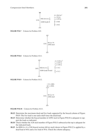
263. 245
Combined Forces on Steel Members
PROBLEMS
Note: In all problems assume the full lateral support conditions.
12.1 A W12×35 section of A992 steel with a single line (along the tensile force) of four 3/4 in.
bolts in the web is subjected to a tensile live load of 65 k and a bending moment only due
to the dead load including the weight of the member along the weak axis of 20 ft.-k. Is this
member satisfactory?
12.2 A W10×33 member is to support a factored tensile force of 100 k and a factored moment
along the x axis of 100 ft.-k including the weight of member. It is a fully welded member
of grade 50 steel. Is the member adequate for the loads?
12.3 A 12 ft. long hanger supports a tensile dead load of 50 k and a live load of 100 k at an
eccentricity of 4 in. with respect to the x axis. Design a W10 section of A992 steel. There
is one line of three bolts of 3/4 in. diameter on one side of the top lange and one line of
three bolts of the same size on the other side of the top lange. The bottom lange has a
bolt pattern similar to the top lange.
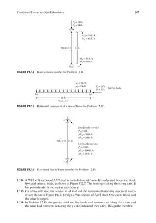
12.4 Design a W8 or W10 member to support the loads shown in Figure P12.1. It has a single
line of four holes for 7/8 in. bolts in the web. The member consists of A992 steel.
12.5 The member in Problem 12.4, in addition to the loading along the x axis, has a factored
bending moment of 40 ft.-k along the y axis. Design the member.
[Hint: Since a sizeable bending along the y axis is involved, initially select a section at
least four times of that required for axial load alone.]
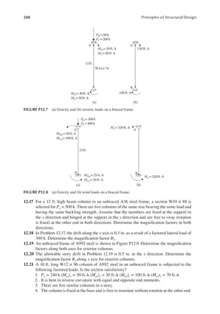
12.6 A horizontal beam section W10×26 of A992 steel is subjected to the service live loads
shown in Figure P12.2. The member is bent about the x axis. Determine the magnitude of
the magniication factor B1.
12.7 A braced frame member W12×58 of A992 steel is subjected to the loads shown in
Figure P12.3. The member is bent about the x axis. Determine the magnitude of the mag-
niication factor B1. Assume pin-end conditions.
12.8 In Problem 12.7, the moments at the ends A and B are both clockwise. The ends are
restrained (ixed). Determine the magniication factor B1.
12.9 In Problem 12.7, in addition to the loads shown a uniformly distributed wind load of 1 k/ft.
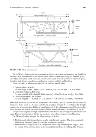
acts laterally between A and B. Determine the magniication factor B1.
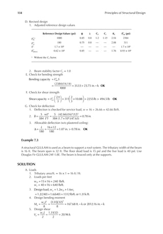
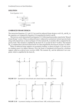
Joist
Joist order span
Standard designation
5N 9F
28G
Depth in inches Number of
joist spaces
Kip load on each panel point
(1 kip= 1000 lbs)
Space
P P P P
2 in.
Depth
8 in.
7½ in.
FIGURE 12.16 Selection of joist girder.

264. 246 Principles of Structural Design
12.10 In Problem 12.7, in addition to the shown x-axis moments, the moments in the y axis at
A and B are as follows. Determine the magniication factor B1.
= =
M M
D y L y
At B( ) 10 ft.-k, ( ) 20ft.-k,both clockwise
= =
M M
D y L y
At A( ) 8ft.-k, ( ) 15ft.-k,both counterclockwise
12.11 The member of a A572 steel section, as shown in Figure P12.4, is used as a beam column
in a braced frame. It is bent about the strong axis. Is the member adequate?
12.12 A horizontal component of a braced frame is shown in Figure P12.5. It is bent about the
strong axis. Is the member adequate? Use A992 steel.
12.13 The member of a A572 steel section, as shown in Figure P12.6, is used as a beam column
in a braced frame. It has restrained ends. Is the member adequate?
15 ft.
(Service loads)
PD= 50 k
wD= 0.5k/ft.
wL= 1 k/ft.
PL= 70k
FIGURE P12.1 Tensile and lexure member for Problem 12.4.
10ft.
30k
30 k
FIGURE P12.2 Compression lexure member for Problem 12.6.
PD= 50 k
MD= 20 ft.-k
ML= 70 ft.-k
MD= 10 ft.-k
ML=40 ft.-k
B
A
PL= 150 k
10 ft.
14 ft.
FIGURE P12.3 Braced frame member for Problem 12.7.

265. 247
Combined Forces on Steel Members
12.14 A W12 × 74 section of A572 steel is part of a braced frame. It is subjected to service, dead,
live, and seismic loads, as shown in Figure P12.7. The bending is along the strong axis. It
has pinned ends. Is the section satisfactory?
12.15 For a braced frame, the service axial load and the moments obtained by structural analy-
sis are shown in Figure P12.8. Design a W14 section of A992 steel. One end is ixed, and
the other is hinged.
12.16 In Problem 12.15, the gravity dead and live loads and moments act along the x axis and
the wind load moments act along the y axis (instead of the x axis). Design the member.
PD= 100 k
PL= 200 k
MD= 20ft.-k
ML= 40ft.-k
MD=30 ft.-k
ML= 50 ft.-k
12 ft.
W12 ×72
FIGURE P12.4 Beam-column member for Problem 12.11.
20 ft.
Service loads
PD= 10 k
wD= 1 k/ft.
wL= 2 k/ft.
PL= 20 k
W10×54
FIGURE P12.5 Horizontal component of a braced frame for Problem 12.12.
Live loads (service)
–
Dead loads (service)
PD= 50 k
MDx= 50 ft.-k
MDy= 20 ft.-k
PL= 100 k
MLx= 100ft.-k
MLy= 30 ft.-k
W14× 68 15ft.
–
FIGURE P12.6 Restrained braced frame member for Problem 12.13.

266. 248 Principles of Structural Design
12.17 For a 12 ft. high beam column in an unbraced A36 steel frame, a section W10 × 88 is
selected for Pu = 500 k. There are ive columns of the same size bearing the same load and
having the same buckling strength. Assume that the members are ixed at the support in
the x direction and hinged at the support in the y direction and are free to sway (rotation
is ixed) at the other end in both directions. Determine the magniication factors in both
directions.
12.18 In Problem 12.17, the drift along the x axis is 0.3 in. as a result of a factored lateral load of
300 k. Determine the magniication factor B2.
12.19 An unbraced frame of A992 steel is shown in Figure P12.9. Determine the magniication
factors along both axes for exterior columns.
12.20 The allowable story drift in Problem 12.19 is 0.5 in. in the x direction. Determine the
magniication factor B2 along x axis for exterior columns.
12.21 A 10 ft. long W12 × 96 column of A992 steel in an unbraced frame is subjected to the
following factored loads. Is the section satisfactory?
1. Pu = 240 k (Mu1)x = 50 ft.-k (Mu1)y = 30 ft.-k (Mu2)x = 100 ft.-k (Mu2)y = 70 ft.-k
2. It is bent in reverse curvature with equal and opposite end moments.
3. There are ive similar columns in a story.
4. The column is ixed at the base and is free to translate without rotation at the other end.
PD=80 k
PL= 200 k
MD= 20 ft.-k
ML= 40 ft.-k
MD= 30 ft.-k
ML= 50 ft.-k
12 ft.
(a) (b)
A
W14× 74
B
A
150ft.-k
100ft.-k
FIGURE P12.7 (a) Gravity and (b) seismic loads on a braced frame.
PD= 200 k
PL= 400k
13 ft.
(a) (b)
A
B
A
B
MDx= 25 ft.-k
MLx=50 ft.-k
MDx= 50ft.-k
MLx= 100 ft.-k
Mx=320ft.-k
Mx= 320ft.-k
FIGURE P12.8 (a) Gravity and (b) wind loads on a braced frame.

267. 249
Combined Forces on Steel Members
12.22 Select a W12 column member of A992 steel of an unbraced frame for the following condi-
tions; all loads are factored:
1. K = 1.2 for the sway case and K = 1 for the unsway case
2. L = 12 ft.
3. Pu = 350 k
4. (Mu1)x = 75 ft.-k
5. (Mu1)y = 40 ft.-k
6. (Mu2)x = 150 ft.-k
7. (Mu2)y = 80 ft.-k
8. Allowable drift = 0.3 in.
9. It has intermediate transverse loading between the ends.
10. Total factored horizontal force = 100 k
11. There are four similar columns in a story.
12.23 An unbraced frame of A992 steel is subjected to dead, live, and wind loads in the
x axis; the wind load causes the sway. Structural analysis provided the loads as shown
in Figure P12.10. Design a W14 section for a maximum drift of 0.5 in. Each column is
subjected to the same axial force and moment.
12.24 A one-story unbraced frame of A992 steel is subjected to dead, roof live, and wind
loads. The bending is in the x axis. Structural analysis provided the loads as shown in
Figure P12.11. The moments at the base are 0. Design a W12 section for a maximum drift
of 0.5 in. The lateral wind load causes the sway.
12.25 Select a K-series open-web steel joist spanning 25 ft. to support a dead load of 30 psf
and a live load of 50 psf. The joist spacing is 3.5 ft. The maximum live load delection is
L/360.
20 ft. 20ft. 20 ft.
W12 ×152 W12×210 W12 ×210 W12 ×152
PD=200 k
PL= 300 k
PD= 100 k
PL=200 k
VL= 200k
(Service load)
PD= 200k
PL=300k
PD= 100k
PL=200 k
14 ft.
(Service
loads)
FIGURE P12.9 Unbraced frame for Problem 12.19.
30 ft.-k
40 ft.-k
(a) (b)
14 ft.
170 k
90 ft.-k
105 ft.-k
400 k
(c)
320 ft.-k
320 ft.-k
176 k
FIGURE P12.10 (a) Dead, (b) live, and (c) wind loads on the unbraced frame for Problem 12.23.

268. 250 Principles of Structural Design
12.26 Select an open-web steel joist for the following looring system:
1. Joist spacing: 3 ft.
2. Span length: 20 ft.
3. Floor slab: 3 in. concrete
4. Other dead load: 30 psf
5. Live load: 60 psf
6. Maximum live load delection: L/240
12.27 On an 18 K 10 joist spanning 30 ft., how much total unit load and unfactored live load in
pounds per square foot can be imposed? The joist spacing is 4 ft. The maximum live load
delection is L/300.
12.28 The service dead load in pounds per square foot on an 18 K 6 joist is one-half of the live
load. What are the magnitudes of these loads on the joist loaded to the capacity at a span
of 20 ft., spaced 4 ft. on center?
12.29 Indicate the joist girder designation for the looring system shown in Figure P12.12.
12.30 For a 30 ft. × 50 ft. bay, joists spaced 3.75 ft. on center, indicate the designation of the joist
girders to be used for a dead load of 20 psf and a live load of 30 psf.
Wind (uplift on roof)
(does not contribute to drift)
MW = –48 ft.-k
PW
= –12 k
ML= 32 ft.-k
MD
=50 ft.-k
PD = 15 k PLr = 25 k
MLr
= 70 ft.-k
16k
Wind loads (pressure on roof)
(lateral)
Dead load Roof live loads
15 ft.
40 ft.
FIGURE P12.11 Dead, roof live, and wind loads on the unbraced frame for Problem 12.24.
DL= 20 psf
LL= 40 psf
(service)
40 ft.
40 ft.
32 ft.
8 ft.
8 ft.
Open-web
joists
Girder
FIGURE P12.12 Open-web joist and joist girder loor system for Problem 12.29.

269. 251
13 Steel Connections
TYPES OF CONNECTIONS AND JOINTS
Most structures’ failure occurs at a connection. Accordingly, the American Institute of Steel
Construction (AISC) has placed a lot of emphasis on connections and has brought out separate
detailed design speciications related to connections in the 2005 Steel Design Manual. Steel con-
nections are made by bolting and welding; riveting is obsolete now. Bolting of steel structures
is rapid and requires less skilled labor. On the other hand, welding is simple and many complex
connections with bolts become very simple when welds are used. But the requirements of skilled
workers and inspections make welding dificult and costly, which can be partially overcome by shop
welding instead of ield welding. When a combination is used, welding can be done in the shop and
bolting in the ield.
Based on the mode of load transfer, the connections are categorized as follows:
1. Simple or axially loaded connection when the resultant of the applied forces passes through
the center of gravity of the connection
2. Eccentrically loaded connection when the line of action of the resultant of the forces does
not pass through the center of gravity of the connection
The following types of joints are formed by the two connecting members:
1. Lap joint: As shown in Figure 13.1, the line of action of the force in one member and the
line of action of the force in the other connecting member have a gap between them. This
causes a bending within the connection, as shown by the dashed lines. For this reason, the
lap joint is used for minor connections only.
2. Butt joint: This provides a more symmetrical loading, as shown in Figure 13.2, that elimi-
nates the bending condition.
The connectors (bolts or welds) are subjected to the following types of forces (and stresses):
1. Shear: The forces acting on the splices shown in Figure 13.3 can shear the shank of the
bolt. Similarly, the weld in Figure 13.4 resists the shear.
2. Tension: The hanger-type connection shown in Figures 13.5 and 13.6 imposes tension in
bolts and welds.
3. Shear and tension combination: The column-to-beam connections shown in Figures 13.7
and 13.8 cause both shear and tension in bolts and welds. The welds are weak in shear and
are usually assumed to fail in shear regardless of the direction of the loading.
BOLTED CONNECTIONS
The ordinary or common bolts, also known as uninished bolts, are classiied as A307 bolts. The
characteristics of A307 steel are very similar to A36 steel. Their strength is considerably less than
those of high-strength bolts. Their use is recommended for structures subjected to static loads and
for the secondary members like purlins, girts, and bracings. With the advent of high-strength bolts,
the use of the ordinary bolts has been neglected, although for ordinary construction, the common
bolts are quite satisfactory.

270. 252 Principles of Structural Design
P P
P
P
FIGURE 13.3 Bolts in shear.
P P
FIGURE 13.4 Welds in shear.
P
FIGURE 13.5 Bolts in tension.
P
FIGURE 13.6 Welds in tension.
P
P
P
P
FIGURE 13.1 Lap joint.
P
P
P
P
2
P
2
FIGURE 13.2 Butt joint.

271. 253
Steel Connections
High-strength bolts have strength that is twice or more of the ordinary bolts. There are two
groups of high-strength bolts: Group A is equivalent to A325-type bolts and Group B is equivalent
to A490-type bolts. High-strength bolts are used in two types of connections: the bearing-type con-
nections and the slip-critical or friction-type connections.
In the bearing-type connection, in which the common bolts can also be used, no frictional resis-
tance in the faying (contact) surfaces is assumed and a slip between the connecting members occurs
as the load is applied. This brings the bolt in contact with the connecting member and the bolt bears
the load. Thus, the load transfer takes place through the bolt.
In a slip-critical connection, the bolts are torqued to a high tensile stress in the shank. This devel-
ops a clamping force on the connected parts. The shear resistance to the applied load is provided by
the clamping force, as shown in Figure 13.9.
P
M
Bolt in shear and tension
FIGURE 13.7 Bolts in shear and tension.
P
M Weld in shear and tension
FIGURE 13.8 Welds in shear and tension.
P
P
Torque applied
Clamping force
μ × Clamping force
P
FIGURE 13.9 Frictional resistance in a slip-critical connection.

272. 254 Principles of Structural Design
Thus, in a slip-critical connection, the bolts themselves are not stressed since the entire force is
resisted by the friction developed on the contact surfaces. For this purpose, the high-strength bolts
are tightened to a very high degree. The minimum pretension applied to bolts is 0.7 times the tensile
strength of steel. These are given in Table 13.1.
The methods available to tighten the bolts comprise (1) the turn of the nut method, (2) the cali-
brated wrench method, (3) the direct tension indicator method, and (4) the twist-off type tension
control method in which bolts are used whose tips are sheared off at a predetermined tension level.
The slip-critical connection is a costly process subject to inspections. It is used for structures
subjected to dynamic loading such as bridges where stress reversals and fatigued loading take place.
For most situations, the bearing-type connection should be used where the bolts can be tightened
to the snug-tight condition, which means the tightness that could be obtained by the full effort of a
person using a spud wrench or the pneumatic wrench.
SPECIFICATIONS FOR SPACING OF BOLTS AND EDGE DISTANCE
1. Deinitions: The following deinitions are given with respect to Figure 13.10.
Gage, g: This is the center-to-center distance between two successive lines of bolts, per-
pendicular to the axis of a member (perpendicular to the load).
Pitch, p: This is the center-to-center distance between two successive bolts along the axis
of a member (in line with the force).
Edge distance, Le: This is the distance from the center of the outermost bolt to the edge of
a member.
2. Minimum spacing: The minimum center-to-center distance for standard, oversized, and
slotted holes should not be less than 22
3 d, but a distance of 3d is preferred; d being the bolt
diameter.
3. Maximum spacing: The maximum spacing of bolts of the painted members or the
unpainted members not subject to corrosion should not exceed 24 times the thickness of
thinner member or 12 in. whichever is less. The maximum spacing for members subject to
corrosion should not exceed 14 times thickness or 7 in. whichever is less.
P
g
Le
FIGURE 13.10 Deinition sketch.
TABLE 13.1
Minimum Pretension on Bolts, k
Bolt Diameter (in.) Area (in.2) Group A, e.g., A325 Bolts Group B, e.g., A490 Bolts
1/2 0.0196 12 15
5/8 0.307 19 24
3/4 0.442 28 35
7/8 0.601 39 49
1 0.785 51 64
1
1
4
1.227 71 102
1
1
2
1.766 103 148

273. 255
Steel Connections
4. Minimum edge distance: The minimum edge distance in any direction are tabulated by the
AISC. It is generally 13
4 times the bolt diameter for the sheared edges and 11
4 times the
bolt diameter for the rolled or gas cut edges.
5. Maximum edge distance: The maximum edge distance should not exceed 12 times the
thickness of the thinner member or 6 in. whichever is less.
BEARING-TYPE CONNECTIONS
The design basis of a connection is as follows:
≤ φ
P R
u n (13.1)
where
Pu is applied factored load on a connection
ϕ is resistance factor = 0.75 for a connection
Rn is nominal strength of a connection
In terms of the nominal unit strength (stress), Equation 13.1 can be expressed as
≤ φ
P F A
u n (13.2)
For bearing-type connections, Fn refers to the nominal unit strength (stress) for the various limit
states or modes of failure and A refers to the relevant area of failure.
The failure of a bolted joint in a bearing-type connection can occur by the following modes:
1. Shearing of the bolt across the plane between the members: In single shear in the lap joint
and in double shear in the butt joint, as shown in Figure 13.11.
For a single shear
=
π
4
2
A d
and for a double shear
=
π
2
2
A d
2. Bearing failure on the contact area between the bolt and the plate, as shown in Figure 13.12.
A d t
= ⋅
P
P
P
P
2
P
2
FIGURE 13.11 Shear failure.
P
P
t
FIGURE 13.12 Bearing failure.

274. 256 Principles of Structural Design
3. Tearing out of the plate from the bolt, as shown in Figure 13.13.
= =
A L t
c
tearing area 2
4. Tensile failure of plate as shown in Figure 13.14. This condition has been discussed in
Chapter 9 for tension members. It is not a part of the connection.
For the shearing type of the limiting state, Fn in Equation 13.2 is the nominal unit shear strength
of bolts, Fnv, which is taken as 50% of the ultimate strength of bolts. The cross-sectional area, Ab,
is taken as the area of the unthreaded part or the body area of bolt. If the threads are in the plane of
shear or are not excluded from shear plane, a factor of 0.8 is applied to reduce the area. This factor
is incorporated in the strength, Fnv.
Thus, for the shear limit state, the design strength is given by
≤ 0.75
P F A n
u nv b b (13.3)
where
Fnv is as given in Table 13.2
Ab = (π/4)d2 for single shear and A = (π/2)d2 for double shear
nb is number of bolts in the connection
In Table 13.2, threads not excluded from shear plane are referred to as the N-type connection,
like 32-N, and threads excluded from shear plane as the X-type connection, like 325-X.
The other two modes of failure, that is, the bearing and the tearing out of a member, are based
not on the strength of bolts but upon the parts being connected. The areas for bearing and tearing
TABLE 13.2
Nominal Unit Shear Strength, Fnv
Bolt Type Fnv (ksi)
A307 27
Group A (e.g., A325-N) threads not excluded from shear plane 54
Group A (e.g., A325-X) threads excluded from shear plane 68
Group B (e.g., A490-N) threads not excluded from shear plane 68
Group B (e.g., A490-X) threads excluded from shear plane 84
P
FIGURE 13.14 Tensile failure of plate.
P Rn
Rn/2
Rn/2
Lc
FIGURE 13.13 Tearing out of plate.

275. 257
Steel Connections
are described in the preceding discussion. The nominal unit strengths in the bearing and the (shear)
tear out depend on the deformation around the holes that can be tolerated and on the types of holes.
The bearing strength is very high because the tests have shown that the bolts and the connected
member actually do not fail in bearing but the strength of the connected parts is impaired. The
AISC expressions combine the bearing and (shear) tear state limits together as follows:
1. For standard, oversized, short-slotted holes and long-slotted holes with slots parallel to the
force where deformation of hole should be ≤0.25 in. (i.e., deformation is a consideration)
= φ ≤ φ
1.2 2.4
P L tF n dtF n
u c u b u b (13.4)
where Fu is ultimate strength of the connected member.
2. For standard, oversized, short-slotted holes and long-slotted holes parallel to the force
where deformations can be >0.25 in. (i.e., deformation is not a consideration)
= φ ≤ φ
1.5 3
P L tF n dtF n
u c u b u b (13.5)
3. For long-slotted holes, slots being perpendicular to the force
= φ ≤ φ
1.0 2.0
P L tF n dtF n
u c u b u b (13.6)
where
ϕ is 0.75
Lc is illustrated in Figure 13.15.
For edge bolt #1
= –
2
L L
h
c e (13.7)
For interior bolt #2
= −
L s h
c (13.8)
where h = hole diameter = (d + 1/8) in.*
In the case of double shear, if the combined thickness of two outside elements is more than the
thickness of the middle element, the middle element is considered for design using twice the bolt
area for shear strength and the thickness of the middle element for bearing strength. However, if
the combined thickness of outer elements is less than the middle element, then the outer element is
considered in design with one-half of the total load, which each outside element shares.
* The AISC stipulates d + 1/16 but 1/8 has been used conservatively.
P
Le
Lc
Lc h
s
#1 #2
FIGURE 13.15 Deinition of Lc.

276. 258 Principles of Structural Design
Example 13.1
A channel section C9 × 15 of A36 steel is connected to a 3/8-in. steel gusset plate, with
7/8-in. diameter, Group A: A325 bolts. A service dead load of 20 k and live load of 50 k is applied
to the connection. Design the connection. The slip of the connection is permissible. The threads
are excluded from the shear plane. Deformation of the hole is a consideration.
SOLUTION
A. The factored load
= + =
1.2(20) 1.6(50) 104 k
Pu
B. Shear limit state
1. Ab = (π/4)(7/8)2 = 0.601 in.2
2. For Group A: A325-X, Fnv = 68 ksi
3. From Equation 13.3
=
= =
No. of bolts
0.75
104
0.75(68)(0.601)
3.39 or 4 bolts
P
F A
u
nv b
C. Bearing limit state
1. Minimum edge distance
=





 =
1
3
4
7
8
1.53in., use 2in.
Le
2. Minimum spacing
s 3
7
8
2.63in.,use 3in.
=





 =
3. h d
1
8
1in.
= + =
4. For holes near edge
= −
= − =
2
2
1
2
1.5in.
L L
h
e e
t = 5/16 in. for the web of the channel section
For a standard size hole of deformation <0.25 in. (deformation is a consideration)
= φ
=





 = ←
Strength/bolt 1.2
1.2(0.75)(1.5)
5
16
(58) 24.5k Controls
L tF
c u
= φ
=











 =
Upper limit 2.4
2.4(0.75)
7
8
5
16
(58) 28.55k
dtFu

277. 259
Steel Connections
5. For interior holes
= − = − =
3 1 2in.
L s h
c
6. =





 =
Strength/bolt 1.2(0.75)(2)
5
16
(58) 32.63k
Upper limit 2.4(0.75)
7
8
5
16
(58) 28.55k Controls
=











 = ←
7. Suppose there are n lines of holes with two bolts in each, then
= = +
=
104 (24.5) (28.55)
1.96
P n n
n
u
= =
Total no. of bolts 2(1.96) 3.92 or 4 bolts
Select four bolts either by shear or bearing.
8. The section has to be checked for the tensile strength and the block shear by the
procedure given in Chapter 9 under the “Tensile Strength of Elements” and “Block
Shear Strength” sections, respectively.
SLIP-CRITICAL CONNECTIONS
In a slip-critical connection, the bolts are not subjected to any stress. The resistance to slip is equal
to the product of the tensile force between the connected parts and the static coeficient of friction.
This is given by
= φ µ
P D h T N n
u u f b s b (13.9)
where
ϕ is a resistance factor with different values as follows:
1. Standard holes and short-slotted holes perpendicular to the direction of load, ϕ = 1
2. Short-slotted holes parallel to the direction of load, ϕ = 0.85
3. Long-slotted holes, ϕ = 0.70
Du is the ratio of installed pretension to minimum pretension; use Du = 1.13, other values
permitted.
μ is the slip (friction) coeficient as given in Table 13.3.
hf is the factor for illers, as follows:
1. No iller or where the bolts have been added to distribute loads in illers, hf = 1
2. One iller between connected parts, hf = 1
3. Two or more illers, hf = 0.85
Tb is minimum bolt pretension given in Table 13.1
Ns is number of slip (shear) planes
nb is number of bolts in the connection
TABLE 13.3
Slip (Friction) Coeficient
Class Surface μ
Class A Unpainted clean mill scale or Class A coating on blast cleaned steel or
hot dipped galvanized and roughened surface
0.30
Class B Unpainted blast cleaned surface or Class B coating on blast cleaned steel 0.5

278. 260 Principles of Structural Design
Although there is no bearing on bolts in a slip-critical connection, the AISC requires that it should
also be checked as a bearing-type connection by Equation 13.3 and a relevant equation out of
Equations 13.4 through 13.6.
Example 13.2
A double-angle tensile member consisting of 2 ∟ 3 × 2½ × 1/4 is connected by a gusset plate
3/4 in. thick. It is designed for a service load of 15 k and live load of 30 k. No slip is permitted.
Use 5/8-in. Group A: A325 bolts and A572 steel. Holes are standard size and bolts are excluded
from the shear plane. There are no illers and the surface is blast cleaned coat A. Deformation of
the hole is a consideration.
SOLUTION
A. Factored design load
= + =
1.2(15) 1.6(30) 66 k
Pu
B. For the slip-critical limit state
1. Du = 1.13
2. Standard holes, ϕ = 1
3. No illers, hf = 1
4. Class A surface, μ = 0.3
5. From Table 13.1, Tb = 19 ksi for 5/8-in. bolts
6. For double shear (double angle), Ns = 2
From Equation 13.9
n
Pu
D h T N
b
u f b s
=
φ µ
= =
66
1
(1.13)(0.3)(1)(19)(2)
5.12
C. Check for the shear limit state as a bearing-type connection
1. Ab = 2(π/4)(5/8)2 = 0.613 in.2
2. For Group A: A325-X, Fnv = 66 ksi
3. From Equation 13.3
=
= =
No. of bolts
0.75
66
0.75(66)(0.613)
2.18
P
F A
u
nv b
D. Check for the bearing limit state as a bearing-type connection
1. Minimum edge distance
=





 =
1
3
4
5
8
1.09 in., use 1.5in.
Le
2. Minimum spacing
s 3
5
8
1.88 in., use 2in.
=





 =

279. 261
Steel Connections
3. h d
1
8
3
4
in.
= + =
4. For holes near edge
= −
= − =
2
1.5
6
16
1.125
L L
h
c e
t = 2(1/4) = 0.5 in. ← thinner than the gusset plate
For a standard size hole of deformation <0.25 in. (deformation is a consideration)
= φ
= = ←
Strength/bolt 1.2
1.2(0.75)(1.125)(0.5)(65) 32.9 k Controls
L tF
c u
= φ
=





 =
Upper limit 2.4
2.4(0.75)
5
8
(0.5)(65) 36.56 k
dtFu
5. For interior holes
= − = −





 =
2
3
4
1.25in.
L s h
c
6. = =
Strength/bolt 1.2(0.75)(1.25)(0.5)(65) 36.56 k
Upper limit 2.4(0.75)
5
8
(0.5)(65) 36.56 k Controls
=





 = ←
7. Suppose there are n lines of holes with two bolts in each, then
= = +
=
66 (32.9) (36.56)
1
P n n
n
u
Total no. of bolts = 2
E. The slip-critical limit controls the design
Number of bolts selected = 6 for symmetry
F. Check for the tensile strength of bolt, as per Chapter 9—”Tensile Strength of Elements” section
G. Check for the block shear, as per Chapter 9—”Block Shear Strength” section
TENSILE LOAD ON BOLTS
This section applies to tensile loads on bolts, in both the bearing type of connections and the
slip-critical connections. The connections subjected to pure tensile loads (without shear) are lim-
ited. These connections exist in hanger-type connections for bridges, lange connections for pip-
ing systems, and wind-bracing systems in tall buildings. A hanger-type connection is shown in
Figure 13.16.
A tension by the external loads acts to relieve the clamping force between the connected parts
that causes a reduction in the slip resistance. This has been considered in the “Combined Shear and
Tensile Forces on Bolts” section. However, as far as the tensile strength of the bolt is concerned, it is
computed without giving any consideration to the initial tightening force or pretension.

280. 262 Principles of Structural Design
The tensile limit state of rupture follows the standard form of Equation 13.2:
≤ ⋅
0.75
T F A n
u nt b b (13.10)
where
Tu is factored design tensile load
Fnt is nominal unit tensile strength as given in Table 13.4
Example 13.3
Design the hanger connection shown in Figure 13.17 for the service dead and live loads of 30 k
and 50 k, respectively. Use Group A: A325 bolts.
SOLUTION
1. Factored design load
= + =
1.2(30) 1.6(50) 116 k
Pu
2. Use 7/8-in. bolt
=
π 




 =
4
7
8
0.601 in.
2
2
Ab
3. From Equation 3.10
=
= =
0.75
116
0.75(90)(0.601)
2.86,use 4 bolts, 2on each side
n
P
F A
b
u
nt b
T T
P
FIGURE 13.16 T-type hanger connection.
TABLE 13.4
Nominal Unit Tensile Strength, Fnt
Bolt Type Fnt (ksi)
A307 45
A325 90
A490 113

281. 263
Steel Connections
COMBINED SHEAR AND TENSILE FORCES ON BOLTS
COMBINED SHEAR AND TENSION ON BEARING-TYPE CONNECTIONS
Many connections are subjected to a combination of shear and tension. A common case is a diago-
nal bracing attached to a column.
When both tension and shear are imposed, the interaction of these two forces in terms of the
combined stress must be considered to determine the capacity of the bolt. A simpliied approach to
deal with this interaction is to reduce the unit tensile strength of a bolt to Fnt
′ (from the original Fnt).
Thus, the limiting state equation is
0.75
T F A n
u nt b b
≤ ′ ⋅ (13.11)
where the adjusted (reduced) nominal unit tensile strength is given as follows:*
′ = −





 ≤
1.3
0.75
F F
F
F
f F
nt nt
nt
nv
v nt (13.12)
where fv is actual shear stress given by the design shear force divided by the area of the number bolts
in the connection.
To summarize, for combined shear and tension in a bearing-type connection, the procedure
comprises the following steps:
1. Use the unmodiied shear limiting state equation (Equation 13.3).
2. Use the tension limiting state equation (Equation 13.11) as a check.
3. Use the relevant bearing limiting state equation from Equations 13.4 through 13.6 as a check.
Example 13.4
A WT12 × 27.5 bracket of A36 steel is connected to a W14 × 61 column, as shown in Figure 13.18,
to transmit the service dead and live loads of 15 and 45 k. Design the bearing-type connection
between the column and the bracket using 7/8-in. Group A: 325-X bolts. Deformation is a
consideration.
* When the actual shear stress fv ≤ 0.3ϕFnv or the actual tensile stress ft ≤ 0.3ϕFnt, the adjustment of Fnt is not required.
FIGURE 13.17 A tensile connection for Example 13.3.

282. 264 Principles of Structural Design
SOLUTION
A. Design data
1. Thickness of bracket = 0.505 in.
2. Thickness of column = 0.645 in.
3. Pu = 1.2 (15) + 1.6 (45) = 90 k
4. Design shear, Vu = Pu (3/5) = 54 k
5. Design tension, Tu = Pu (4/5) = 72 k
B. For the shear limiting state
1. Ab = (π/4)(7/8)2 = 0.601 in.2
2. For Group A, A325-X, Fnv = 68 ksi
3. From Equation 13.3
=
= =
0.75
54
0.75(68)(0.601)
1.762 bolts
n
V
F A
b
n
nv b
Use four bolts, two on each side (minimum two bolts on each side)
C. For the tensile limiting state
1. Fnt = 90 ksi
2. Actual shear stress
= = =
54
(0.601)(4)
22.46 ksi
f
V
A n
v
u
b b
3. Adjusted unit tensile strength from Equation 13.12
′ = −





 ≤
= − =
1.3
0.75
1.3(90)
90
0.75(68)
(22.46) 77.36 ksi
F F
F
F
f F
nt nt
nt
nv
v nt
OK
4. From Equation 13.11
=
′
= = <
0.75
72
0.75(77.36)(0.601)
2.06 4 bolts
n
T
F A
b
u
nt b
OK
3
PD =15 k
PL =45 k
4
FIGURE 13.18 Column-bracket connection for Example 13.4.

283. 265
Steel Connections
D. Check for the bearing limit state
1. Minimum edge distance
=





 =
1
3
4
7
8
1.53in., use 2in.
Le
2. Minimum spacing
s 3
7
8
2.63in., use 3in.
=





 =
3. h d
1
8
1in.
= + =
4. For holes near edge
= −






= −





 =
2
2
1
2
1.5in.
L L
h
e e
t = 0.505 in. ← thickness of WT lange
For a standard size hole of deformation <0.25 in. (deformation is a consideration)
( )( )( )( )( )
= φ
= = ← >
Strength 1.2
1.2 0.75 1.5 0.505 58 4 158 k controls 54 k
L tF n
c u b
OK
= φ
=





 =
Upper limit 2.4
2.4(0.75)
7
8
(0.505)(58)(4) 184.5 k
dtF n
u b
COMBINED SHEAR AND TENSION ON SLIP-CRITICAL CONNECTIONS
As discussed in the “Tensile Load on Bolts” section, the externally applied tension tends to reduce
the clamping force and the slip-resisting capacity. A reduction factor ks is applied to the previously
described slip-critical strength. Thus, for the combined shear and tension, the slip-critical limit
state is
= φ µ
V D h T N n k
u u f b s b s (13.13)
where
=
−
1
k
T
D T n
s
u
u b b (13.14)
Vu is factored shear load on the connection
Tu is factored tension load on the connection
Tb is minimum bolt pretension given in Table 13.1
Ns is number of slip (shear) planes
nb is number of bolts in the connection
hf is a factor for illers deined in Equation 13.9
μ is slip (friction) coeficient as given is Table 13.3

284. 266 Principles of Structural Design
Combining Equations 13.13 and 13.14, the relation for the number of bolts is
=
φµ
+






1
n
D T
V
h
T
b
u b
u
f
u (13.15)
To summarize, for the combined shear and tension in a slip-critical connection, the procedure
is as follows:
1. Use the shear limiting state equation (Equation 13.3).*
2. Use the (original) tensile limit state equation (Equation 13.10).
3. Use the relevant bearing limiting state equation from Equations 13.4 through 13.6 as a check.
4. Use the (modiied) slip-critical limit state equation (Equation 13.13).
Example 13.5
Design Example 13.4 as a slip-critical connection. The holes are standard size. There is no iller.
The surface is unpainted clean mill scale.
SOLUTION
A. Design loads from Example 13.4
1. Vu = 54 k
2. Tu = 72 k
B. For the shear limiting state
nb = 1.762 from Example 13.4 (use four bolts, min. two on each side)
C. For the tensile limiting state
=
= = <
0.75
72
0.75(90)(0.601)
1.77 4 bolts
n
T
F A
b
u
nt b
OK
D. For the bearing limit state
( )
= > K OK
Strength 158 k from Example 13.4 54
E. For the slip-critical limit state
1. Standard holes, ϕ = 1
2. No iller, hf = 1
3. Class A surface, μ = 0.3
4. From Table 13.1, Tb = 39 ksi
5. For single shear, Ns = 1
6. From Equation 13.15
=
φµ
+






= +






=
1
1
1.13(39)
54
(1)(0.3)(1)
72
5.72 bolts (select 6 bolts, 3 on each side of web)
n
D T
V
h
T
b
u b
u
f
u
* The slip-critical connections also are required to be checked for bearing capacity and shear strength.

285. 267
Steel Connections
WELDED CONNECTIONS
Welding is a process in which the heat of an electric arc melts the welding electrode and the adjacent
material of the part being connected simultaneously. The electrode is deposited as a iller metal
into the steel, which is referred to as the base metal. There are two types of welding processes. The
shielded metal arc welding (SMAW), usually done manually, is the process used for ield welding.
The submerged arc welding (SAW) is an automatic or semiautomatic process used in shop welding.
The strength of a weld depends on the weld metal used, which is the strength of the electrode used.
An electrode is speciied by the letter E followed by the tensile strength in ksi and the last two digits
specifying the type of coating. Since strength is a main concern, the last two digits are speciied by
XX, a typical designation being E 70 XX. The electrode should be selected to have a larger tensile
strength than the base metal (steel). For steel of 58 ksi strength, the electrode E 70 XX is used, and
for 65 ksi steel, the electrode E 80 XX is used. Electrodes of high strength E 120 XX are available.
The two common types of welds are illet welds and grove or the butt welds, as shown in
Figure 13.19. Groove welds are stronger and more expensive than illet welds. Most of the welded
connections are made by illet welds because of a larger allowed tolerance.
The codes and standards for welds are prepared by the American Welding Society. These have
been adopted in the AISC Manual 2010.
GROOVE WELDS
EFFECTIVE AREA OF GROOVE WELD
The effective area of a complete-joint-penetration (CJP) groove weld is the length times the thick-
ness of the thinner part joined.
The effective area of a partial-joint-penetration (PJP) groove weld is the length times the depth
(effective throat) of the groove.* The minimum effective throat for PJP weld has been listed in the AISC
Manual 2010. It is 1/8 in. for 1/4 in. material thickness to 5/8 in. for over 6 in. thick material joined.
FILLET WELDS
EFFECTIVE AREA OF FILLET WELD
The cross section of a illet weld is assumed to be a 45° right angle triangle, as shown in Figure 13.20.
Any additional buildup of weld is neglected. The size of the illet weld is denoted by the sides of the
triangle, w, and the throat dimension, given by the hypotenuse, t, which is equal to 0.707w. When
the SAW process is used, the greater heat input produces a deeper penetration.
The effective throat size is taken as follows:
= = 0.707
T t w
e (13.16)
MINIMUM SIZE OF FILLET WELD
The minimum size should not be less than the dimension shown in Table 13.5.
* For gas metal arc and lux cored arc, the groove depth is subtracted by 1/8 in.
(a)
Complete penetration Partial penetration
(b)
FIGURE 13.19 Types of welds: (a) illet and (b) groove of butt welds.

286. 268 Principles of Structural Design
MAXIMUM SIZE OF FILLET WELD
1. Along the edges of material less than 1/4 in. thick, the weld size should not be greater than
the thickness of the material.
2. Along the edges of material 1/4 in. or more, the weld size should not be greater than the
thickness of the material less 1/4 in.
LENGTH OF FILLET WELD
1. The effective length of end-loaded illet weld, LE, is equal to the actual length for the length
up to 100 times the weld size. When the length exceeds 100 times the weld size, the actual
length is multiplied by a reduction factor β = 1.2 – 0.002 (l/w), where l is actual length and w
is weld size. When the length exceeds 300 times the weld size, the effective length is 180 w.
2. The minimum length should not be less than four times the weld size.
3. If only the longitudinal welds are used, the length of each side should not be less than the
perpendicular distance between the welds.
STRENGTH OF WELD
COMPLETE JOINT PENETRATION GROOVE WELDS
Since the weld metal is always stronger than the base metal (steel), the strength of a CJP groove weld
is taken as the strength of the base metal. The design of the connection is not done in the normal sense.
For the combined shear and tension acting on a CJP groove weld, there is no explicit approach.
The generalized approach is to reduce the tensile strength by a factor of (fv/Ft)2 subject to a maxi-
mum reduction of 36% of the tensile strength.
PARTIAL JOINT PENETRATION WELDS AND FILLET WELDS
A weld is weakest in shear and is always assumed to fail in the shear mode. Although a length of
weld can be loaded in shear, compression, or tension, the failure of a weld is assumed to occur in the
shear rupture through the throat of the weld. Thus,
= φ
P F A
u w w (13.17)
P
Throat
f= 0.707w
Leg
P
Leg
w
w
45°
FIGURE 13.20 Fillet weld dimensions.
TABLE 13.5
Minimum Size of Weld (in.)
Base Material Thickness of Thinner Part (in.) w (in.)
≤1/4 1/8
>1/4 to ≤1/2 3/16
>3/4 to ≤3/4 1/4
>3/4 5/16

287. 269
Steel Connections
where
ϕ is resistance factor = 0.75
Fw is strength of weld = 0.6FEXX
FEXX is strength of electrode
Aw is effective area of weld = TeL
However, there is a requirement that the weld shear strength cannot be larger than the base metal
shear strength. For the base metal, the shear yield and shear rupture strengths are taken to be 0.6 times
the tensile yield of steel and 0.6 times the ultimate strength of steel, respectively. The yield strength
is applied to the gross area and the rupture strength to the net area of shear surface, but in the case of
a weld, both areas are the same. The resistance factor is 1 for shear yield and 0.75 for shear rupture.
Thus, the PJP groove and the illet welds should be designed to meet the strengths of the weld
and the base metal, whichever is smaller, as follows:
1. Weld shear rupture limit state
By the substitution of the terms in Equation 13.17
=
P F T L
u e E
0.45 EXX (13.18)
where
FEXX is strength of electrode, ksi
LE is effective length of weld
Te is effective throat dimension from Equation 13.16
2. Base metal shear limit state
a. Shear yield strength
=
P F T L
u y e E
0.60 (13.19)
where t is thickness of thinner connected member
b. Shear rupture strength
=
P F T L
u u e E
0.45 (13.20)
In addition, the block shear strength should also be considered by Equation 9.7.
Example 13.6
A tensile member consisting of one ∟ 3½ × 3½ × 1/2 section carries a service dead load of 30 k
and live load of 50 k, as shown in Figure 13.21. A single 3/4-in. plate is directly welded to the
column lange using the CJP groove. Fillet welds attach the angles to the plate. Design the welded
connection. The longitudinal length of the weld cannot exceed 5 in. Use the return (transverse)
weld, if necessary. Use E70 electrodes. The steel is A36.
SOLUTION
A. Angle plate (bracket) connection
1. Factored load
= + =
1.2(30) 1.6(50) 116 k
Pu
2. Maximum weld size. For thinner member, thickness of angle, t = 1/2 in.
w t
1
16
7
16
in.
= −





 =

288. 270 Principles of Structural Design
3. Throat dimension, SMAW process
=





 =
0.707
7
16
0.309 in.
Te
4. For weld shear limit state, from Equation 13.18
L
P
F T
E
u
e
=
= = ←
0.45
116
0.45(70)(0.309)
11.92 in. ~12 in. controls
EXX
5. For steel shear yield limit state, from Equation 13.19
L
P
F t
E
u
y
=
=






=
0.6
116
0.6(36)
1
2
10.74 in.
6. For steel rupture limit state, from Equation 13.20
L
P
F t
E
u
u
=
=






=
0.45
116
0.45(58)
1
2
8.9 in.
7. Provide a 5-in.-long weld on each side* (maximum in this problem) with 1 in. return on
each side.
8. The longitudinal length of welds (5 in.) should be at least equal to the transverse distance
between the longitudinal weld (31/2); OK
9. Length of 12 in. greater than 4w of 1.75 in. OK
* Theoretically, the lengths on two sides are unequally distributed so that the centroid of the weld passes through the center
of gravity of the angle member.
30°
5 in. max
P
FIGURE 13.21 Column-bracket welded connection for Example 13.6.

289. 271
Steel Connections
B. Column-bracket connection
1. The connection is subjected to tension and shear as follows:
T P
V P
u u
u u
= ° = ° =
= ° = ° =
cos 30 116 cos 30 100.5k
sin 30 116 sin 30 58 k
2. For the CJP groove, the design strengths are the same as for the base metal.
3. This is the case of the combined shear and tension in groove weld. Using a maximum
reduction of 36%,* tensile strength = 0.76Ft.
4. For the base material tensile limit state
T F tL t
L
u t
= φ
=






(0.76 ) , where is gusset plate thickness
100.5 0.9(0.76)(36)
3
4
or
L 5.44 in. Controls
= ←
Use 6 in. weld length
5. For the base metal shear yield limit state
V F tL
L
u y
=
=






0.6
58 0.6(36)
3
4
or
3.6 in.
L =
6. For the base metal shear rupture limit state
V F tL
L
u u
=
=






0.45
58 0.45(58)
3
4
or
3.0 in.
L =
FRAME CONNECTIONS
There are three types of beam-to-column frame connections:
1. FR (fully restrained) or rigid frame or moment frame connection
It transfers the full joint moment and shear force.
It retains the original angle between the members or rotation is not permitted.
2. Simple or pinned frame or shear frame connection
It transfers shears force only.
It permits rotation between the members.
3. PR (partially restrained) frame connection
It transfers some moment and the entire shear force.
It permits a speciied amount of rotation.
* See the “Complete Joint Penetration Groove Welds” section.

290. 272 Principles of Structural Design
The relationship between the applied moment and the rotation (variation of angle) of members
for rigid, semirigid, and simple framing is shown in Figure 13.22.
A fully rigid joint will have a small change in angle with the application of moment. A simple
joint will be able to support some moment (although theoretically the moment capacity should be
zero). A semirigid joint is where the actual moment and rotation are accounted for.
SHEAR OR SIMPLE CONNECTION FOR FRAMES
There are a variety of beam-to-column or beam-to-girder connections that are purposely made lex-
ible for rotation at the ends of the beam. These are designed for the end reaction (shear force). These
are used for structures where the lateral forces due to wind or earthquake are resisted by the other
systems like truss framing or shear walls. Following are the main categories of simple connections.
SINGLE-PLATE SHEAR CONNECTION OR SHEAR TAB
This is a simple and economical approach that is becoming very popular. The holes are prepunched
in a plate and in the web of the beam to be supported. The plate is welded (usually shop welded)
to the supporting column or beam. The prepunched beam is bolted to the plate at the site. This is
shown in Figure 13.23.
FRAMED-BEAM CONNECTION
The web of the beam to be supported is connected to the supporting column through a pair of
angles, as shown in Figure 13.24.
SEATED-BEAM CONNECTION
The beam to be supported sits on an angle attached to the supporting column lange, as shown in
Figure 13.25.
END-PLATE CONNECTION
A plate is welded against the end of the beam to be supported. This plate is then bolted to the sup-
porting column or beam at the site. This is shown in Figure 13.26. These connections are becoming
popular but not as much as the single-plate connection.
Moment
Rotation
Rigid
Semirigid
Simple
FIGURE 13.22 Moment-rotation characteristics.

291. 273
Steel Connections
FIGURE 13.23 Single-plate or shear tab connection.
Bolted or welded
Pair of angles
FIGURE 13.24 Framed-beam connection.
Bolted or welded
FIGURE 13.25 Seated-beam connection.

292. 274 Principles of Structural Design
The design of the simple connections proceeds along the lines of the bearing-type connec-
tions described in the “Bearing-Type Connections” section. The limiting states considered are as
follows: (1) shear on bolts; (2) bearing yield strength; (3) shear rupture strength between the bolt
and the connected part, as discussed in the “Bearing-Type Connections” section; and (4) block
shear strength of the connected part.
The AISC Manual 2010 includes a series of tables to design the different types of bolted and
welded connections. The design of only a single-plate shear connection for frames is presented here.
SINGLE-PLATE SHEAR CONNECTION FOR FRAMES
The following are the conventional conigurations for a single-plate shear connection:
1. A single row of bolts comprising 2–12 bolts.
2. The distance between the bolt line and weld line should not exceed 3.5 in.
3. Provision of the standard or short-slotted holes.
4. The horizontal distance to edge Le ≥ 2db (bolt diameter).
5. The plate and beam must satisfy t ≤ (db/2) + (1/16).
6. For welded connections, the weld shear rupture and the base metal shear limits should be
satisied.
7. For bolted connections, the bolt shear, the plate shear, and the bearing limit states should
be satisied.
8. The block shear of the plate should be satisfactory.
Example 13.7
Design a single-plate shear connection for a W14 × 82 beam joining a W12 × 96 column by a
3/8-in. plate, as shown in Figure 13.27. The factored reaction at the support of the beam is 50 k.
Use 3/4-in.-diameter Group A: A325-X bolts, A36 steel, and E70 electrodes.
SOLUTION
A. Design load
P R
u u
= = 50 k
B. For W14 × 82
d t t b
F F
f w f
y u
= = = =
= =
14.3in., 0.855in., 0.51in., 14.7 in.
36 ksi, 58 ksi
FIGURE 13.26 End-plate connection.

293. 275
Steel Connections
C. For W12 × 96
d t t b
F F
f w f
y u
= = = =
= =
12.7 in., 0.9 in., 0.55in., 12.2in.
36 ksi, 58 ksi
D. Column plate–welded connection
1. For 3/8-in. plate
t
Weld max size
1
16
3
8
1
16
5
16
in.
= −





 =





 −





 =






2. Te = 0.707 (5/16) = 0.22 in.
3. The weld shear limit state, from Equation 13.18
L
P
F T
E
u
e
( )( )
=
= = ←
0.45
50
0.45 70 0.22
7.21 in. ~ 8 in. controls
EXX
4. The steel shear yield limit state, from Equation 13.19
L
P
F t
u
y
=
=






= <
0.6
50
0.6(36)
3
8
6.17 8 in.
5. The steel rupture limit state, from Equation 13.20
L
P
F t
u
u
=
=






= <
0.45
50
0.45(58)
3
8
5.1. in 8 in.
W12× 96
W14 ×82
-in. plate
3
8
FIGURE 13.27 Single-plate connection for Example 13.7.

294. 276 Principles of Structural Design
6. Up to 100 times of the weld size (in this case 100 (5/16) = 31.25 in.), effective length is
equal to actual length, hence L = LE = 8 in.
7. L w
of 8 in. > 4 of 1.25 in. OK
E. Beam plate–bolted connection
E.1 The single shear limit state
1. Ab = (π/4)(3/4)2 = 0.441 in.2
2. For A325-X, Fnv = 68 ksi
3. From Equation 13.3
P
F A
u
nv b
=
= =
No. of bolts
0.75
50
0.75(68)(0.441)
2.22 or 3 bolts
E.2 The bearing limit state
1. Minimum edge distance
L d
e b
= =





 =
1
3
4
1
3
4
3
4
1.31in., use 1.5 in.
2. Minimum spacing
s db
= =





 =
3 3
3
4
2.25in., use 2.5 in.
3. h d
1
8
7
8
in.
= + =
4. For holes near edge
L L
h
c e
=






= −





 =
–
2
1.5
7
16
1.063in.
t = 3/8 in. thinner member
For a standard size hole of deformation <0.25 in.
L tF
c u
Strength/bolt 1.2
1.2(0.75)(1.063)
3
8
(58) 20.81k Controls
= φ
=





 = ←
dtFu
= φ
=











 =
Upper limit 2.4
2.4(0.75)
3
4
3
8
(58) 29.36 k
5. For other holes
L s h
c = − = −





 =
2.5
7
8
1.625in.
6. Strength/bolt 1.2(0.75)(1.625)
3
8
(58) 31.81k
=





 =

295. 277
Steel Connections
Upper limit 2.4(0.75)
3
4
3
8
(58) 29.36 k Controls
=











 = ←
7. Total strength for three bolts–two near edges
OK
Pu = + = >
2(20.81) 29.36 71k 50 k
8. The section has to be checked for block shear by the procedure given in Chapter 9.
MOMENT-RESISTING CONNECTION FOR FRAMES
Fully restrained (rigid) and partially restrained (semirigid) are two types of moment-resisting con-
nections. It is customary to design a semirigid connection for some speciic moment capacity, which
is less than the full moment capacity.
Figure 13.28 shows a moment-resisting connection that has to resist a moment, M, and a shear
force (reaction), V.
The two components of the connection are designed separately. The moment is transmitted to the
column lange as a couple by the two tees attached at the top and bottom langes of the beam. This
results in tension, T, on the top lange and compression, C, on the bottom lange.
From the couple expression, the two forces are given by
= =
C T
M
d
(13.21)
where d is taken as the depth of the beam.
The moment is taken care of by designing the tee connection for the tension T. It should be noted
that the magnitude of the force T can be decreased by increasing the distance between the tees (by
a deeper beam).
The shear load is transmitted to the column by the beam–web connection. This is designed as
a simple connection of the type discussed in the “Shear or Simple Connection for Frames” section
through single plate, two angles (framed), or seat angle.
The connecting tee element is subjected to prying action as shown in Figure 13.29. This prying
action could be eliminated by connecting the beam section directly to the column through a CJP
groove weld, as shown in Figure 13.30.
Stiffeners
(if required)
Tee section
V
M
Web angle
FIGURE 13.28 Moment-resisting connection.

296. 278 Principles of Structural Design
The welded length should not exceed beam lange width, bf, of both the beam and the column,
otherwise a thicker plate has to be welded at the top and bottom of the beam.
Example 13.8
Design the connection of Example 13.7 as a moment-resisting connection subjected to a factored
moment of 200 ft.-k and a factored end shear force (reaction) of 50 k. The beam langes are groove
welded to the column.
SOLUTION
A. Design for the shear force has been done in Example 13.7.
B. Flanges welded to the column
1. C T
M
d
200(12)
14.3
167.83k
= =
= =
2. The base material limit state
T FytL t t
u f
= φ =
, where
T/2
T
T/2
FIGURE 13.29 Prying action in connection.
CJP groove weld
FIGURE 13.30 Welded moment-resisting connection.

297. 279
Steel Connections
or
L
T
Fyt
b
u
f
=
φ
= = <
167.83
(0.9)(36)(0.855)
6.06 in.
Provide a 6-in.-long CJP weld.
PROBLEMS
13.1 Determine the strength of the bearing-type connection shown in Figure P13.1. Use A36
steel, Group A: A325, 7/8-in. bolts. The threads are not excluded from shear plane.
Deformation of the hole is a consideration.
13.2 Determine the strength of the bearing-type connection shown in Figure P13.2. Use A36
steel, Group A: A325, 7/8-in. bolts. The threads are excluded from shear plane. Deformation
of holes is not a consideration.
P
in.
1
2
2 in. 3 in. 3 in. 2 in.
2 in.
4 in.
4 in.
2 in.
7
8
-in. bolts
FIGURE P13.1 Connection for Problem 13.1.
P
P
2
in.
1
2
7
8
P
2
P
2
2 in. 3 in. 3 in. 2 in.
2 in.
4 in.
4 in.
2 in.
1¼ in.
-in. bolts
FIGURE P13.2 Connection for Problem 13.2.

298. 280 Principles of Structural Design
13.3 Design the bearing-type connection for the bolt joint shown in Figure P13.3. The steel is
A572 and the bolts are Group A: A325, 3/4-in. diameter. The threads are excluded from
shear plane. Deformation of holes is a consideration.
13.4 A chord of a truss shown in Figure P13.4 consists of 2 C9 × 20 of A36 steel connected by
a 1-in. gusset plate. Check the bearing-type connection by Group B: A490 bolts assuming
threads are excluded from shear plane. Deformation of holes is not a consideration.
13.5 Design the bearing-type connection shown in Figure P13.5 (threads excluded from shear
plane) made with 7/8-in. Group B: A490 bolts. Use A572 steel. Deformation of holes is a
consideration.
13.6 Solve Problem 13.1 for the slip-critical connection of unpainted clean mill scale surface.
The holes are standard size and there are no illers.
13.7 Solve Problem 13.2 for the slip-critical connection of unpainted blast cleaned surface. The
holes are standard size. Two illers are used between connected members.
13.8 Design a slip-critical connection for the plates shown in Figure P13.6 to resist service dead
load of 30 k and live load of 50 k. Use 1-in. Group A: A325 bolts and A572 steel. Assume
painted class A surface. The holes are standard size. There are no illers. The threads are
excluded from shear plane and hole deformation is a consideration.
PD = 100k
PL = 150k
(service loads)
-in. plate
-in. plate
-in. diameter bolts
1
2
3
4
3
4
FIGURE P13.3 Connection for Problem 13.3.
PD = 40 k
PL = 100 k
(service loads)
-in. dia
5
8
FIGURE P13.4 Truss chord connection for Problem 13.4.
-in. bolts
-in. thickness
W14 × 48
PD = 100 k
PL = 130 k
(service loads)
7
8
3
4
FIGURE P13.5 Connection for Problem 13.5.

299. 281
Steel Connections
13.9 A single angle 3½ × 3 × 1/4 tensile member is connected by a 3/8-in.-thick gusset plate.
Design a no-slip (slip-critical) connection for the service dead and live loads of 8 and
24 k, respectively. Use 7/8-in. Group A: A325 bolts and A36 steel. Assume an unpainted
blast cleaned surface. The holes are standard size. There is one iller. The threads are not
excluded from shear plane and the hole deformation is not a consideration.
13.10 A tensile member shown in Figure P13.7 consisting of two ∟ 4 × 3½ × 1/2 carries a wind
load of 176 k acting at 30°. A bracket consisting of a tee section connects this tensile
member to a column lange. The connection is slip-critical. Design the bolts for the tensile
member only. Use 7/8-in. Group B: A490-X bolts and A572 steel. Assume an unpainted
blast cleaned surface. The holes are short-slotted parallel to the direction of loading.
There are no illers and hole deformation is not a consideration.
13.11 Determine the strength of the bolts in the hanger connection shown in Figure P13.8
(neglect the prying action).
13.12 Are the bolts in the hanger connection adequate in Figure P13.9?
13.13 A WT12 × 31 is attached to a 3/4-in. plate as a hanger connection, to support service dead
and live loads of 25 and 55 k, respectively. Design the connection for 7/8-in. Group A:
A325 bolts and A572 steel (neglect the prying action).
9-in. × -in. plate
P
P
-in. plate
5
8
5
8
FIGURE P13.6 Connection for Problem 13.8.
WT8 × 50
W14 × 82
30°
P = 176
4 × 3½ ×
1
2
FIGURE P13.7 Connection for Problem 13.10.

300. 282 Principles of Structural Design
In Problems 13.14 through 13.16, the threads are excluded from shear planes and defor-
mation is a consideration.
13.14 Design the column-to-bracket connection from Problem 13.10. Slip is permitted.
13.15 In the bearing-type connection shown in Figure P13.10, determine the load capacity, Pu.
13.16 A tensile member is subjected to service dead and live loads of 30 and 50 k, respectively,
through 7/8-in. plate, as shown in Figure P13.11. Design the bearing-type connection. The
steel is A572 and the bolts are 3/4-in., Group B: A490-X.
In Problems 13.17 through 13.19, the connecting surface is unpainted clean mill scale. The holes
are standard size and there are no illers.
13.17 Design the connection from Problem 13.14 as the slip-critical connection.
13.18 Solve Problem 13.15 as the slip-critical connection.
-in. A325
Group A
Steel A572
4 × 3½ ×
3
4
1
2
2
PD = 10 k
PL = 15 k
(service loads)
FIGURE P13.9 Hanger-type connection for Problem 13.12.
8 – -in.
3
4
Group B, A490–X bolts
A572 steel
WT 12 × 34
W 12 × 58
P
3
4
FIGURE P13.10 Combined shear-tension connection for Problem 13.15.
-in. bolts A490
Group B
Steel A572
7
8
FIGURE P13.8 Hanger-type connection for Problem 13.11.

301. 283
Steel Connections
13.19 Design the connection in Problem 13.16 as the slip-critical connection. Bolts are preten-
sioned to 40 k.
13.20 Determine the design strength of the connection shown in Figure P13.12. The steel is
A572 and the electrodes are E 70.
13.21 In Problem 13.20, the applied loads are a dead load of 50 k and a live load of 150 k. For
the welding shown in Figure P13.12, determine the thickness of the plates.
13.22 A 1/4-in.-thick lat plate is connected to a gusset plate of 5/16-in. thickness by a 3/16-in.
weld as shown in Figure P13.13. The maximum longitudinal length is 4 in. Use the return
(transverse) weld, if necessary. The connection has to resist a dead load of 10 k and live
load of 20 k. What is the length of the weld? Use E 70 electrodes. The steel is A36.
13.23 Two 1/2 × 10-in. A36 plates are to be connected by a lap joint for a factored load of 80 k. Use
E 80 electrodes. The steel is A36. Determine the weld size for the entire width (transverse)
welding of the plate.
13.24 The plates in Problem 13.23 are welded as a partial-joint-penetration butt connection.
The minimum effective throat width according to AISC speciications is 3/16 in. Design
the connection.
4 bolts
45°
Design -in. bolt connection
3
4
FIGURE P13.11 Combined shear-tension connection for Problem 13.16.
10 in.
15 × plate
Plate 8 ×
-in. weld
8 in.
1
2
1
2
7
16
FIGURE P13.12 Welded connection for Problem 13.20.

302. 284 Principles of Structural Design
13.25 Design the longitudinal illet welds to connect a ∟ 4 × 3 × 1/2 angle tensile member
shown in Figure P13.14 to resist a service dead load of 50 k and live load of 80 k. Use E
70 electrodes. The steel is A572.
13.26 A tensile member consists of 2 ∟ 4 × 3 × 1/2 carries a service dead load of 50 k and live
load of 100 k, as shown in Figure P13.15. The angles are welded to a 3/4-in. gusset plate,
which is welded to a column lange. Design the connection of the angles to the gusset
plate and the gusset plate to the column. The gusset plate is connected to the column by a
CJP groove and the angles are connected by a illet weld. Use E 70 electrodes. The steel
is A572.
13.27 Design a single-plate shear connection for a W14 × 53 beam joining a W14 × 99 column
by a 1/4-in. plate. The factored reaction is 60 k. Use A36 steel. Use 5/8-in. Group A: A325
bolts and E70 welds.
13.28 Design a single-plate shear connection for a W16 × 67 beam joining a W18 × 71 column
by a 1/2-in. plate to support a factored beam reaction of 70 k. Use 3/4-in. Group B: A490
bolts and E80 welds. The beam and columns have A992 steel and the plate is A36 steel.
5 in. P
Maximum 4 in.
FIGURE P13.13 Welded connection for Problem 13.22.
WT section
4 × 3 × 1
2
FIGURE P13.14 Welded connection for Problem 13.25.

303. 285
Steel Connections
13.29 Design the connection for Problem 13.26 as a moment connection to resist a factored
moment of 200 ft.-k in addition to the factored reaction of 60 k.
13.30 Design the connection for Problem 13.27 as a moment-resisting connection to resist a
factored moment of 300 ft.-k and a factored shear force of 70 k.
Design welded connection
4 × 3½
40°
-in. gusset plate
3
4
FIGURE P13.15 Welded connection for Problem 13.26.

305. Section IV
Reinforced Concrete Structures

307. 289
14 Flexural Reinforced
Concrete Members
PROPERTIES OF REINFORCED CONCRETE
Concrete is a mixture of cement, sand, gravel, crushed rock, and water. Water reacts with cement
in a chemical reaction known as hydration that sets the cement with other ingredients into a solid
mass, high in compression strength. The strength of concrete depends on the proportion of the
ingredients. The most important factor for concrete strength is the water–cement ratio. More water
results in a weaker concrete. However, an adequate amount is needed for concrete to be workable
and easy to mix. An adequate ratio is about 0.25 by weight. The process of selecting the relative
amounts of ingredients for concrete to achieve a required strength at the hardened state and to be
workable in the plastic (mixed) state is known as concrete mix design. The speciication of con-
crete in terms of the proportions of cement, ine (sand) aggregate, and coarse (gravel and rocks)
aggregate is called the nominal mix. For example, a 1:2:4 nominal mix has one part cement, two
parts sand, and four parts gravel and rocks by volume. Nominal mixes having the same proportions
could vary in strength. For this reason, another expression for speciication known as the standard
mix uses the minimum compression strength of concrete as a basis. The procedure for designing
a concrete mix is a trial-and-error method. The irst step is to ix the water–cement ratio for the
desired concrete strength using an empirical relationship between the compressive strength and
the water–cement ratio. Then, based on the characteristics of the aggregates and the proportion-
ing desired, the quantities of the other materials comprising cement, ine aggregate, and coarse
aggregate are determined.
There are some other substances that are not regularly used in the proportioning of the mix.
These substances, known as mixtures, are usually chemicals that are added to change certain char-
acteristics of concrete such as accelerating or slowing the setting time, improving the workability of
concrete, and decreasing the water–cement ratio.
Concrete is quite strong in compression, but it is very weak in tension. In a structural system,
the steel bars are placed in the tension zone to compensate for this weakness. Such concrete is
known as reinforced concrete. At times, steel bars are also used in the compression zone to gain
extra strength with a leaner concrete size as in reinforced concrete columns and doubly reinforced
beams.
COMPRESSION STRENGTH OF CONCRETE
The strength of concrete varies with time. The speciied compression strength denoted as fc′ is the
value that concrete attains 28 days after the placement. Beyond that stage, the increase in strength
is very small. The strength fc′ ranges from 2500 to 9000 psi with a common value between 3000
and 5000 psi.
The stress–strain diagram of concrete is not linear to any appreciable extent; thus, concrete does
not behave elastically over a major range. Moreover, concrete of different strengths have stress–
strain curves that have different slopes. Therefore, in concrete, the modulus of elasticity cannot be
ascertained directly from a stress–strain diagram.

308. 290 Principles of Structural Design
The American Concrete Institute (ACI), which is a primary agency in the United States that
prepares the national standards for structural concrete, provides the empirical relations for the mod-
ulus of elasticity based on the compression strength, fc′.
Although the stress–strain curves have different slopes for concrete of different strengths, the
following two characteristics are common to all concretes:
1. The maximum compression strength, fc′, in all concrete is attained at a strain level of
approximately 0.002 in./in.
2. The point of rupture of all curves lies in the strain range of 0.003–0.004 in./in. Thus, it is
assumed that concrete fails at a strain level of 0.003 in./in.
DESIGN STRENGTH OF CONCRETE
To understand the development and distribution of stress in concrete, let us consider a simple rect-
angular beam section with steel bars at the bottom (in the tensile zone), which is loaded by an
increasing transverse load.
The tensile strength of concrete being small, the concrete will soon crack at the bottom at a
low transverse load. The stress at this level is known as the modulus of rupture, and the bending
moment is referred to as the cracking moment. Beyond this level, the tensile stress will be handled
by the steel bars and the compression stress by the concrete section above the neutral axis. Concrete
being a brittle (not a ductile) material, the distribution of stress within the compression zone could
be considered linear only up to a moderate load level when the stress attained by concrete is less
than 1/2 fc′, as shown in Figure 14.1. In this case, the stress and strain bear a direct proportional
relationship.
As the transverse load increases further, the strain distribution will remain linear (Figure 14.2b)
but the stress distribution will acquire a curvilinear shape similar to the shape of the stress–strain
curve. As the steel bars reach the yield level, the distribution of strain and stress at this load will be
as shown in Figure 14.2b and c.
εs
εc
fc =εc Ec
fs=εsEs
(a) (b) (c)
FIGURE 14.1 Stress–strain distribution at moderate loads: (a) section, (b) strain, and (c) stress.
εc
fc
′
0.85fc
′
c
a
fy fy
(a) (b) (c) (d)
fy /E
FIGURE 14.2 Stress–strain distribution at ultimate load: (a) section, (b) strain, (c) stress, and (d) equivalent
stress.

309. 291
Flexural Reinforced Concrete Members
For simpliication, Whitney (1942) proposed a ictitious but equivalent rectangular stress
distribution of intensity 0.85fc′, as shown in Figure 14.2d. This has since been adopted by the ACI.
The property of this rectangular block of depth a is such that the centroid of this rectangular block
is the same as the centroid of actual curved shape and that the area under the two diagrams in
Figure 14.2c and d are the same. Thus, for design purposes, the ultimate compression of concrete is
taken to be 0.85fc′, uniformly distributed over the depth, a.
STRENGTH OF REINFORCING STEEL
The steel bars used for reinforcing are round, deformed bars with some form of patterned ribbed
projections onto their surfaces. The bar sizes are designated from #3 through #18. For #3 to #8
sizes, the designation represents the bar diameter in one-eighths of an inch, that is, the #5 bar has a
diameter of 5/8 in. The #9, #10, and #11 sizes have diameters that provide areas equal to the areas
of the 1 in. × 1 in. square bar, 11
8 in. × 11
8 in. square bar, and 11
4 in. × 11
4 in. square bar, respec-
tively. Sizes #14 and #18 are available only by special order. They have diameters equal to the areas
of a11
2 in. ×11
2 in. square bar and 2 in. × 2 in. square bar, respectively. The diameter, area, and unit
weight per foot for various sizes of bars are given in Appendix D, Table D.1.
The most useful properties of reinforcing steel are the yield stress, fy and the modulus of elasticity, E.
A large percentage of reinforcing steel bars is not made from new steel but is rolled from melted,
reclaimed steel. These are available in different grades. Grade 40, Grade 50, and Grade 60 are
common, where Grade 40 means the steel having a yield stress of 40 ksi and so on. The modulus
of elasticity of reinforcing steel of different grades varies over a very small range. It is adopted as
29,000 ksi for all grades of steel.
Concrete structures are composed of the beams, columns, or column–beam types of structures
where they are subjected to lexure, compression, or the combination of lexure and compression.
The theory and design of simple beams and columns have been presented in the book.
LOAD RESISTANCE FACTOR DESIGN BASIS OF CONCRETE
Until mid-1950, concrete structures were designed by the elastic or working stress design (WSD)
method. The structures were proportioned so that the stresses in concrete and steel did not exceed
a fraction of the ultimate strength, known as the allowable or permissible stresses. It was assumed
that the stress within the compression portion of concrete was linearly distributed. However, beyond
a moderate load when the stress level is only about one-half the compressive strength of concrete,
the stress distribution in a concrete section is not linear.
In 1956, the ACI introduced a more rational method wherein the members were designed for
a nonlinear distribution of stress and the full strength level was to be explored. This method was
called the ultimate strength design (USD) method. Since then, the name has been changed to the
strength design method.
The same approach is known as the load resistance factor design (LRFD) method in steel and
wood structures. Thus, concrete structures were the irst ones to adopt the LFRD method of design
in the United States.
ACI Publication No. 318, revised numerous times, contains the codes and standards for concrete
buildings. ACI 318-56 of 1956 for the irst time included the codes and standards for USD in an
appendix to the code. ACI 318-63 provided equal status to WSD and USD methods, bringing both
of them within the main body of the code. ACI 318-02 code made USD, with the name changed to
the strength design method, the mandatory method of design. ACI 318-11 provides the latest design
provisions.
In the strength design method, the service loads are ampliied using the load factors. The
member’s strength at failure, known as the theoretical or the nominal capacity, is somewhat reduced

310. 292 Principles of Structural Design
by a strength reduction factor to represent the usable strength of the member. The ampliied loads
must not exceed the usable strength of member, namely,
Amplified loads on member Usable strength of member
≤ (14.1)
Depending upon the type of structure, the loads are the compression forces, shear forces, or
bending moments.
REINFORCED CONCRETE BEAMS
A concrete beam is a composite structure where a group of steel bars are embedded into the tension
zone of the section to support the tensile component of the lexural stress. The areas of the group of
bars are given in Appendix D, Table D.2. The minimum widths of beam that can accommodate a
speciied number of bars in a single layer are indicated in Appendix D, Table D.3. These tables are
very helpful in designs.
Equation 14.1 in the case of beams takes the following form similar to wood and steel structures:
M M
u n
≤ φ (14.2)
where
Mu is maximum moment due to the application of the factored loads
Mn is nominal or theoretical capacity of the member
φ is strength reduction (resistance) factor for lexure
According to the lexure theory, Mn = FbS, where Fb is the ultimate bending stress and S is the sec-
tion modulus of the section. The application of this formula is straightforward for a homogeneous
section for which the section modulus or the moment of inertia could be directly found. However,
for a composite concrete–steel section and a nonlinear stress distribution, the lexure formula pres-
ents a problem. A different approach termed the internal couple method is followed for concrete
beams.
In the internal couple method, two forces act on the beam cross section represented by a com-
pressive force, C, acting on one side of the neutral axis (above the neutral axis in a simply supported
beam) and a tensile force, T, acting on the other side. Since the forces acting on any cross section of
the beam must be in equilibrium, C must be equal and opposite of T, thus representing a couple. The
magnitude of this internal couple is the force (C or T) times the distance Z between the two forces
called the moment arm. This internal couple must be equal and opposite to the bending moment
acting at the section due to the external loads. This is a very general and convenient method for
determining the nominal moment, Mn, in concrete structures.
DERIVATION OF THE BEAM RELATIONS
The stress distribution across a beam cross section at the ultimate load is shown in Figure 14.3 rep-
resenting the concrete stress by a rectangular block as stated in the “Design Strength of Concrete”
section.
The ratio of stress block and depth to the neutral axis is deined by a factor 1
β as follows:
a
c
1
β = (14.3)
Suficient test data are available to evaluate 1
β . According to the ACI

311. 293
Flexural Reinforced Concrete Members
fc
1. For 4000 psi 0.85
1
′ ≤ β = (14.4a)
f
f
c
c
2. For 4000 psi but 8000 psi
0.85
4000
1000
(0.05)
1
′ > ≤
β = −
′−






(14.4b)
′ > β =
f
3. For 8000 psi 0.65
1 (14.4c)
With reference to Figure 14.3, since force = (stress)(area),
C f ab
c
(0.85 )( )
= ′ (a)
T f A
y s
= (b)
Since C = T,
f ab f A
c y s
(0.85 )( )
′ = (c)
or
a
A f
f b
s y
c
0.85
=
′
(d)
or
a
f d
f
y
c
0.85
=
ρ
′
(14.5)
where
A
bd
s
steelratio
ρ = = (14.6)
Since moment = (force)(moment arm),
M T d
a
f A d
a
n y s
2 2
= −




= −



 (e)
Substituting a from Equation 14.5 and As from Equation 14.6 into (e), we obtain
M f bd
f
f
n y
y
c
1
1.7
2
= ρ −
ρ
′





 (f)
0.85fc
′
c
fy T
a
b
d
d
C
h
Z
a/2
FIGURE 14.3 Internal forces and couple acting on a section.

312. 294 Principles of Structural Design
Substituting (f) into Equation 14.2 at equality, we obtain
M
bd
f
f
f
u
y
y
c
1
1.7
2
φ
= ρ −
ρ
′





 (14.7)
Equation 14.7 is a very useful relation for analysis and design of a beam.
If we arbitrarily deine the expression on the right side of Equation 14.7 as K, called the coeficient
of resistance, then Equation 14.7 becomes
M bd K
u
2
= φ (14.8)
where
K f
f
f
y
y
c
1
1.7
= ρ −
ρ
′





 (14.9)
The coeficient K depends on (1) ρ, (2) fy, and (3) fc′. The values of K for different combinations of
ρ, fy, and fc′ are listed in Appendix D, Tables D.4 through D.10.
In place of Equation 14.7, these tables can be directly used in beam analyses and designs.
STRAIN DIAGRAM AND MODES OF FAILURE
The strain diagrams in Figures 14.1 and 14.2 show a straight line variation of the concrete compres-
sion strain εC to the steel tensile strain, εS; the line passes through the neutral axis. Concrete can
have a maximum strain of 0.003 and the strain at which steel yields is εy = fy /E. When the strain dia-
gram is such that the maximum concrete strain of 0.003 and the steel yield strain of εy are attained at
the same time, it is said to be a balanced section, as shown by the solid line labeled I in Figure 14.4.
In this case, the amount of steel and the amount of concrete balance each other out and both of
these will reach the failing level (will attain the maximum strains) simultaneously. If a beam has
more steel than the balanced condition, then the concrete will reach a strain level of 0.003 before
the steel attains the yield strain of εy. This is shown by condition II in Figure 14.4. The neutral axis
moves down in this case.
The failure will be initiated by crushing of concrete, which will be sudden since concrete is
brittle. This mode of failure in compression is undesirable because a structure will fail suddenly
without any warning.
0.003
NA at under-reinforced condition
Balanced
neutral axis (NA)
NA at over-reinforced condition
II
I
III
εy=
fy
E
FIGURE 14.4 Strain stages in a beam.

313. 295
Flexural Reinforced Concrete Members
If a beam has lesser steel than the balanced condition, then steel will attain its yield strain
before the concrete can reach the maximum strain level of 0.003. This is shown by condition III in
Figure 14.4. The neutral axis moves up in this case. The failure will be initiated by the yielding of
the steel, which will be gradual because of the ductility of steel. This is a tensile mode of failure,
which is more desirable because at least there is an adequate warning of an impending failure.
The ACI recommends the tensile mode of failure or the under-reinforcement design for a concrete
structure.
BALANCED AND RECOMMENDED STEEL PERCENTAGES
To ensure the under-reinforcement conditions, the percent of steel should be less than the balanced
steel percentage, ρb, which is the percentage of steel required for the balanced condition.
From Figure 14.4, for the balanced condition,
c
f E
d c
y
0.003 /
=
−
(a)
By substituting c = a/ 1
β from Equation 14.3 and a f d f
y c
/0.85
= ρ ′ from Equation 14.5 and E = 29 ×
106 psi in Equation (a), the following expression for the balanced steel is obtained:
f
f f
b
c
y y
0.85 870,000
87,000
1
ρ =
β ′





 +





 (14.10)
The values for the balanced steel ratio, ρb, calculated for different values of fc′ and fy are tabulated in
Appendix D, Table D.11. Although a tensile mode of failure ensues when the percent of steel is less
than the balanced steel, the ACI code deines a section as tension controlled only when the tensile
strain in steel t
ε is equal to or greater than 0.005 as the concrete reaches its strain limit of 0.003. The
strain range between f E
y y
( / )
ε = and 0.005 is regarded as the transition zone.
The values of the percentage of steel for which t
ε is equal to 0.005 are also listed in Appendix D,
Table D.11 for different grades of steel and concrete. It is recommended to design beams with a
percentage of steel that is not larger than these listed values for t
ε of 0.005.
If a larger percentage of steel is used than for t 0.005
ε = , to be in the transition region, the
strength reduction factor φ should be adjusted, as discussed in the “Strength Reduction Factor for
Concrete” section.
MINIMUM PERCENTAGE OF STEEL
Just as the maximum amount of steel is prescribed to ensure the tensile mode of failure, a minimum
limit is also set to ensure that the steel is not too small so as to cause failure by rupture (cracking)
of the concrete in the tension zone. The ACI recommends the higher of the following two values for
the minimum steel in lexure members:
A
f
f
bd
s
c
y
( )
3
min =
′
(14.11)
or
A
f
bd
s
y
( )
200
min = (14.12)

314. 296 Principles of Structural Design
where
b is width of beam
d is effective depth of beam
The values of ρmin, which is (As)min/bd, are also listed in Appendix D, Table D.11, where a higher of
the values from Equations 14.10 and 14.11 have been tabulated.
The minimum amount of steel for slabs is controlled by shrinkage and temperature require-
ments, as discussed in the “Speciications for Slabs” section.
STRENGTH REDUCTION FACTOR FOR CONCRETE
In Equations 14.2 and 14.7, a strength reduction factor φ is applied to account for all kinds of uncer-
tainties involved in strength of materials, design and analysis, and workmanship. The values of the
factor recommended by the ACI are listed in Table 14.1.
For the transition region between the compression-controlled and the tension-controlled stages
when t
ε is between εy (assumed to be 0.002) and 0.005 as discussed above, the value of φ is interpo-
lated between 0.65 and 0.9 by the following relation:
t
0.65 ( 0.002)
250
3
φ = + ε − 





*
(14.13)
The values† of εt for different percentages of steel are also indicated in Appendix D, Tables D.4
through D.10. When it is not listed in these tables, it means that εt is larger than 0.005.
SPECIFICATIONS FOR BEAMS
The ACI speciications for beams are as follows:
1. Width-to-depth ratio: There is no code requirement for b/d ratio. From experience, the
desirable b/d ratio lies between 1/2 and 2/3.
2. Selection of steel: After a required reinforcement area is computed, Appendix D, Table D.2
is used to select the number of bars that provide the necessary area.
3. The minimum beam widths required to accommodate multiples of various size bars are
given in Appendix D, Table D.3. This is an useful design aid as demonstrated in the example.
4. The reinforcement is located at a certain distance from the surface of the concrete called
the cover. The cover requirements in the ACI code are extensive. For beams, girders, and
columns that are not exposed to weather or are not in contact with the ground, the mini-
mum clear distance from the bottom of the steel to the concrete surface is 1½ in. There is a
* For spiral reinforcement this is t 0.002)(250 3).
φ = 0.70 + (ε −
†
t
ε is calculated by the formula f f
t c y
(0.00255 ) 0.003
1
ε = ′β ρ − .
TABLE 14.1
Strength Reduction Factors
Structural System φ
1. Tension-controlled beams and slabs 0.9
2. Compression-controlled columns
Spiral 0.70
Tied 0.65
3. Shear and torsion 0.75
4. Bearing on concrete 0.65

315. 297
Flexural Reinforced Concrete Members
minimum cover requirement of 11
2 in. from the outermost longitudinal bars to the edge
toward the width of the beam, as shown in Figure 14.5.
5. Bar spacing: The clear spacing between the bars in a single layer should not be less than
any of the following:
• 1 in.
• The bar diameter
• 11
3 × maximum aggregate size
6. Bars placement: If the bars are placed in more than one layer, those in the upper layers
are required to be placed directly over the bars in the lower layers and the clear distance
between the layers must not be less than 1 in.
7. Concrete weight: Concrete is a heavy material. The weight of the beam is signiicant. An
estimated weight should be included. If it is found to be appreciably less than the weight of
the section designed, then the design should be revised. For a good estimation of concrete
weight, Table 14.2 could be used as a guide.
ANALYSIS OF BEAMS
Analysis relates to determining the factored or service moment or the load capacity of a beam of
known dimensions and known reinforcement.
The analysis procedure follows:
1. Calculate the steel ratio from Equation 14.6:
A
bd
s
ρ =
Effective
depth
Hook
Hanger
Stirrup (see chapter 15)
Main reinforcement
Clear cover
Bar spacing
Clear
cover
FIGURE 14.5 Sketch of beam speciications.
TABLE 14.2
First Estimate of Beam Weight
Design Moment, Mu (ft.-k) Estimated Weight (lb/ft.)
≤200 300
>200 but ≤300 350
>300 but ≤400 400
>400 but ≤500 450
>500 500

316. 298 Principles of Structural Design
2. Calculate (As)min from Equations 14.11 and 14.12 or use Appendix D, Table D.11. Compare
this to the As of the beam to ensure that it is more than the minimum.
3. For known ρ, read t
ε from Appendix D, Tables D.4 through D.10 or by the formula in the
footnote of Equation 14.13. If no value is given, then t 0.005.
ε = If t 0.005,
ε < determine φ
from Equation 14.13.
4. For known ρ, compute K from Equation 14.9 or read the value from Appendix D, Tables
D.4 through D.10.
5. Calculate Mu from Equation 14.7:
M bd K
u
2
= φ
6. Break down into the loads if required.
Example 14.1
The loads on a beam section are shown in Figure 14.6. Determine whether the beam is adequate
to support the loads. f f
c y
4,000 psi and 60,000 psi.
′ = =
SOLUTION
A. Design loads and moments
1. Weight of beam/ft. = (12/12) × (20/12) × 1 × 150 = 250 lb/ft. or 0.25 k/ft.
2. Factored dead load, wu = 1.2 (1.25) = 1.5 k/ft.
3. Factored live load, Pu = 1.6 (15) = 24 k
4. Design moment due to dead load = wuL2/8 = 1.5(20)2/8 = 75 ft.-k
5. Design moment due to live load = PuL/4 = 24(20)/4 = 120 ft.-k
6. Total design moment, Mu = 195 ft.-k
7. As = 3.16 in.2 (from Appendix D, Table D.2 for 4 bars of size #8)
8. ρ = As/bd = 3.16/12 × 17 = 0.0155
9. (As)min = 0.0033 (from Appendix D, Table D.11) < 0.0155 OK
10. t 0.005
ε ≥ (value not listed in Appendix D, Table D.9), φ = 0.9
11. K = 0.8029 ksi (for ρ = 0.0155 from Appendix D, Table D.9)
12. M bd K
u OK
(0.9)(12)(17) (0.8029) 2506in.-kor 209ft.-k 195ft.-k
2 2
= φ = = >
20 in.
17 in.
12 in.
20 ft.
DL=1 k/ft.
(excluding weight)
LL= 15 k
4–#8
FIGURE 14.6 Beam for Example 14.1.

317. 299
Flexural Reinforced Concrete Members
DESIGN OF BEAMS
In wood beam design in Chapter 7 and steel beam design in Chapter 11, beams were designed for
bending moment capacity and checked for shear and delection.
In concrete beams, shear is handled independently, as discussed in Chapter 16. For delection,
the ACI stipulates that when certain depth requirements are met, delection will not interfere with
the use or cause damage to the structure. These limiting values are given in Table 14.3 for normal
weight (120–150 lb/ft.3) concrete and Grade 60 steel. For other grade concrete and steel, the adjust-
ments are made as indicated in the footnotes to Table 14.3.
When the minimum depth requirement is met, delection needs not be computed. For members
of lesser thickness than those listed in Table 14.3, the delections should be computed to check for
safe limits. This book assumes that the minimum depth requirement is satisied.
Beam design falls into the two categories discussed below.
DESIGN FOR REINFORCEMENT ONLY
When a beam section has been ixed from architectural or any other consideration, only the amount
of steel has to be selected. The procedure is as follows:
1. Determine the design moment, Mu including the beam weight for various critical load
combinations.
2. Using d = h – 3 and φ = 0.9, calculate the required K from Equation 14.8 expressed as
K
M
bd
u
2
=
φ
3. From Appendix D, Tables D.4 through D.10, ind the value ofρcorresponding to K of step 2.
From the same tables, conirm that t 0.005.
ε ≥ If t 0.005,
ε < reduce φ by Equation 14.13,
recompute K, and ind the corresponding ρ.
4. Compute the required steel area As from Equation 14.6:
A bd
s = ρ
5. Check for the minimum steel As(min) from Appendix D, Table D.11.
6. Select the bar size and the number of bars from Appendix D, Table D.2. From Appendix D,
Table D.3, check whether the selected steel (size and number) can it into width of the
beam, preferably in a single layer. They can be arranged in two layers. Check to conirm
that the actual depth is at least equal to h − 3.
7. Sketch the design.
TABLE 14.3
Minimum Thickness of Beams and Slabs for Normal Weight Concrete and Grade 60 Steel
Minimum Thickness, h (in.)
Member Simply Supported Cantilever One End Continuous Both Ends Continuous
Beam L/16 L/18.5 L/21 L/8
Slab (one-way) L/20 L/24 L/28 L/10
Notes: L is the span in inches.
For lightweight concrete of unit weight 90–120lb/ft.3, the table values should be multiplied by (1.65 – 0.005Wc) but not less
than 1.09, where Wc is the unit weight in lb/ft.3
For other than Grade 60 steel, the table value should be multiplied by (0.4 + fy /100), where fy is in ksi.

318. 300 Principles of Structural Design
Example 14.2
Design a rectangular reinforced beam to carry a service dead load of 1.6 k/ft. and a live load of 1.5
k/ft. on a span of 20 ft. The architectural consideration requires the width to be 10 in. and depth
to be 24 in. Use f f
c y
3,000 psi and 60,000 psi.
′ = =
SOLUTION
1. Weight of beam/ft. = (10/12)(24/12) × 1 × 150 = 250 lb/ft. or 0.25 k/ft.
2. wu = 1.2 (1.6 + 0.25) + 1.6 (1.5) = 4.62 k/ft.
3. Mu = wuL2/8 = 4.62(20)2/8 = 231 ft.-k or 2772 in.-k
4. d = 24 − 3 = 21 in.
5. 2772 (0.9)(10)(21) 0.698 ksi
2
K = =
6. = 0.0139
ρ t 0.0048 (from Appendix D, Table D.6)
ε =
7. From Equation 14.13, = 0.65+ (0.0048 - 0.002)(250 3) = 0.88
φ
8. Revised K = =
2772 (0.88)(10)(21) 0.714 ksi
2
9. Revised ρ = 0.0143 (from Appendix D, Table D.6)*
10. A bd
s = (0.0143)(10)(21) = 3in.2
= ρ
11. As(min) = 0.0033 (from Appendix D, Table D.11) < 0.0143 OK
12. Selection of steel
13. The beam section is shown in Figure 14.7.
DESIGN OF BEAM SECTION AND REINFORCEMENT
The design comprises determining the beam dimensions and selecting the amount of steel. The
procedure is as follows:
1. Determine the design moment, Mu, including the beam weight for various critical load
combinations.
2. Select the steel ratio ρ corresponding to ε =
t 0.005 from Appendix D, Table D.11.
3. From Appendix D, Tables D.4 through D.10, ind K for the steel ratio of step 2.
* For K 0.714 ksi, 0.0046.
t
= ε = ϕ will need a minor adjustment again.
Bar Size No. of Bars As, from Appendix D, Table D.2
Minimum Width in One Layer from
Appendix D, Table D.3
#6 7 3.08 15 NG
#7 5 3.0 12.5 NG
#9 3 3.0 9.5 OK
Select three bars of #9
21 in.
3–#9
Stirrups
(not designed)
3 in.
10 in.
FIGURE 14.7 Beam section for Example 14.2.

319. 301
Flexural Reinforced Concrete Members
4. For b/d ratio of 1/2 and 2/3, ind two values of d from the following expression:
d
M
b d K
u
( / )
1/3
=
φ






*
(14.14)
5. Select the effective depth to be between the two values of step 4
6. If the depth from Table 14.3 is larger, use that value.
7. Determine the corresponding width b from
b
M
d K
u
2
=
φ
(14.15)
8. Estimate h and compute the weight of the beam. If this is excessive as compared to the
assumed value of step 1, repeat steps 1 through 7
9. From now on, follow steps 4 through 7 of the design procedure in the “Design for
Reinforcement Only” section for the selection of steel.
Example 14.3
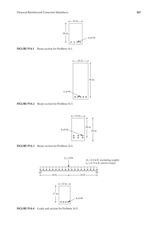
Design a rectangular reinforced beam for the service loads shown in Figure 14.8. Use
f f
c y
3,000 psi and 60,000 psi.
′ = =
SOLUTION
1. Factored dead load, wu = 1.2(1.5) = 1.8 k/ft.
2. Factored live load, Pu = 1.6(20) = 32 k
3. Design moment due to dead load = wuL2/8 = 1.8(30)2/8 = 202.5 ft.-k
4. Design moment due to live load = PuL/3 = 32(30)/3 = 320 ft.-k
5. Total moment, Mu = 522.5 ft.-k
6. Weight of beam from Table 14.2, 0.5 k/ft.
7. Factored dead load including weight 1.2(1.5 + 0.5) = 2.4 k/ft.
8. Moment due to dead load = 2.4(30)2/8 = 270 ft.-k
9. Total design moment = 590 ft.-k or 7080 in.-k
10. ρ = 0.0136 (from Appendix D, Table D.11 for t
ε = 0.005)
11. K = 0.684 ksi (from Appendix D, Table D.6)
12.
13. Depth for delection (from Table 14.3)
h
L
16
30 12
16
22.5 in.
= =
×
=
or d = h – 3 = 22.5 – 3 = 19.5 in.
Use d = 27 in.
* This relation is the same as Mu bd2 K or M b d d K
u ( ) .
3
= φ
Select b/d ratio Calculate d from Equation 14.14
1/2 28.3a
2/3 25.8
a [7080/0.9(1/2)(0.684)]1/3

320. 302 Principles of Structural Design
14. From Equation 14.15
= =
b
7080
(0.9)(27) (0.684)
15.75in.,use 16 in.
2
15. h = d + 3 = 30 in.
Weight of beam/ft. = (16/12)(30/12) × 1 × 150 = 500 lb/ft. or 0.50 k/ft. OK
16. bd
s
Α = ρ = =
(0.0136)(16)(27) 5.88 in.2
17. Selection of steel
27 in.
5–#10
bars
Stirrups
(not designed)
3 in.
16 in.
PL
3
= 320 ft.-k
= 270 ft.-k
wuL2
8
10 ft. 10 ft. 10 ft.
DL=1.5 k/ft.
(excluding weight)
LL= 20 k
LL = 20 k
FIGURE 14.8 Loads, bending moments, and beam section for Example 14.3.
Bar Size No. of Bars
As, from
Appendix D,
Table D.2
Minimum Width in One
Layer from Appendix D,
Table D.3
#9 6 6.00 16.5 NG
#10 5 6.35 15.5
Select ive bars of #10

321. 303
Flexural Reinforced Concrete Members
ONE-WAY SLAB
Slabs are the concrete loor systems supported by reinforced concrete beams, steel beams, concrete
columns, steel columns, concrete walls, or masonry walls. If they are supported on two opposite
sides only, they are referred to as one-way slabs because the bending is in one direction only, per-
pendicular to the supported edge. When slabs are supported on all four edges, they are called two-
way slabs because the bending is in both directions. A rectangular loor plan has slab supported
on all four sides. However, if the long side is two or more times of the short side, the slab could be
considered a one-way slab spanning the short direction.
A one-way slab is analyzed and designed as 12 in. wide beam segments placed side by side hav-
ing a total depth equal to the slab thickness, as shown in Figure 14.9.
The amount of steel computed is considered to exist in 12 in. width on average. Appendix D,
Table D.12 is used for this purpose; it indicates for the different bar sizes the center-to-center spacing
of the bars for a speciied area of steel. The relationship is as follows:
Bar spacing center to center
Requiredsteelarea
Areaof1bar
12
= × (14.16)
SPECIFICATIONS FOR SLABS
The ACI speciications for one-way slab follow:
1. Thickness: Table 14.3 indicates the minimum thickness for one-way slabs where
deflections are not to be calculated. The slab thickness is rounded off to the nearest
1/4 in. on the higher side for slabs up to 6 in. and to the nearest 1/2 in. for slabs thicker
than 6 in.
2. Cover: (1) For slabs that are not exposed to the weather or are not in contact with the
ground, the minimum cover is 3/4 in. for #11 and smaller bars and (2) for slabs exposed to
the weather or in contact with the ground, the minimum cover is 3 in.
3. Spacing of bars: The main reinforcement should not be spaced on center to center more
than (1) three times the slab thickness or (2) 18 in., whichever is smaller.
4. Shrinkage steel: Some steel is placed in the direction perpendicular to the main steel to
resist shrinkage and temperature stresses. The minimum area of such steel is
a. For Grade 40 or 50 steel, shrinkage As = 0.002bh.
b. For Grade 60 steel, shrinkage As = 0.0018bh, where b = 12 in.
h
Shrinkage steel
Main steel
1
2
i
n
.
FIGURE 14.9 Simply supported one-way slab.

322. 304 Principles of Structural Design
The shrinkage and temperature steel should not be spaced farther apart than (1) ive
times the slab thickness or (2) 18 in., whichever is smaller.
5. Minimum main reinforcement: The minimum amount of main steel should not be less than
the shrinkage and temperature steel.
ANALYSIS OF ONE-WAY SLAB
The analysis procedure is as follows:
1. For the given bar size and spacing, read As from Appendix D, Table D.12.
2. Find the steel ratio:
where 12in., 0.75in. 1/2 (bar diameter)
A
bd
b d h
s
ρ = = = − − *
3. Check for the minimum shrinkage steel and also that the main reinforcement As is more
than As(min):
= 0.002
(min)
A bh
s
4. For ρ of step 2, read K and t
ε (if given in the same appendices) from Appendix D, Tables
D.4 through D.10.
5. Correct φ from Equation 14.13 if t 0.005
ε < .
6. Find out Mu as follows and convert to loads if necessary:
M bd K
u
2
= φ
Example 14.4
The slab of an interior loor system has a cross section as shown in Figure 14.10. Determine
the service live load that the slab can support in addition to its own weight on a span of 10 ft.
f f
c y
3,000 psi, 40,000 psi.
′ = =
SOLUTION
1. As = 0.75 in.2 (from Appendix D, Table D.12)
2. d = (6 − 1/2)(0.75) = 5.625 in. and ρ= As/bd = 0.75/(12) (5.625) = 0.011
3. As(min) = 0.002bh = (0.002)(12)(6.75) = 0.162 < 0.75 in.2 OK
4. K = 0.402 (from Appendix D, Table D.4), εt > 0.005 for ρ = 0.011
5. Mu = ϕbd2 K = =
(0.9)(12)(5.625) (0.402) 137.37 in.-k or 11.45 ft.-k
2
6. Mu = wuL2/8 or wu = 8Mu/L2 = 8(11.45)/102 = 0.916 k/ft.
7. Weight of a slab/ft. = (12/12)(6.75/12)(1)(150/1000) = 0.084 k/ft.
8. wu = 1.2(wD) + 1.6(wL) or 0.916 = 1.2(0.084) + 1.6 wL or wL = 0.51 k/ft.
Since the slab width is 12 in., live load is 0.51 k/ft.2
* For slabs laid on the ground, d = h − 3 − 1/2 (bar diameter).
#6 bars at 7 in. OC
3/4 in.
6 in.
FIGURE 14.10 Cross section of slab of a loor system (perpendicular to span) for Example 14.4.

323. 305
Flexural Reinforced Concrete Members
DESIGN OF ONE-WAY SLAB
1. Determine the minimum h from Table 14.3. Compute the slab weight/ft. for b = 12 in.
2. Compute the design moment Mu. The unit load per square foot automatically becomes
load/ft. since the slab width = 12 in.
3. Calculate an effective depth, d, from
= − − ×
d h cover 1/2 assumed bar diameter
4. Compute K assuming ϕ = 0.90,
K
M
bd
u
2
=
φ
5. From Appendix D, Tables D.4 through D.10, ind the steel ratio ρ and note the value of t
ε
(if t
ε is not listed then t
ε > 0.005)
6. If t 0.005,
ε < correct φ from Equation 14.13 and repeat steps 4 and 5
7. Compute the required As:
ρ
A bd
s =
8. From the table in Appendix D, Table D.12, select the main steel satisfying the condition
that the bar spacing is ≤3h or 18 in.
9. Select shrinkage and temperature of steel:
A bh
s
Shrinkage 0.002 Grade 40 or 50 steel
( )
=
or
bh
0.0018 Grade 60 steel
( )
10. From Appendix D, Table D.12, select size and spacing of shrinkage steel with a maximum
spacing of 5h or 18 in., whichever is smaller.
11. Check that the main steel area of step 7 is not less than the shrinkage steel area of step 9.
12. Sketch the design.
Example 14.5
Design an exterior one-way slab exposed to the weather to span 12 ft. and to carry a service dead
load of 100 pounds per square foot (psf) and live load of 300 psf in addition to the slab weight.
Use f f
c y
3,000 psi and 40,000 psi.
′ = =
SOLUTION
1. Minimum thickness for delection from Table 14.3
20
12(12)
20
7.2in.2
h
L
= = =
For exterior slab use h = 10 in.
2. Weight of slab = (12/12)(10/12)(1)(150/1000) = 0.125 k/ft.
3. wu = 1.2(0.1 + 0.125) + 1.6(0.3) = 0.75 k/ft.
4. Mu = wuL2/8 = 13.5 ft.-k or 162 in.-k
5. Assuming #8 size bar (diameter = 1 in.)
d h – cover –1/2 bar diameter
10 – 3 –1/ 2 1 6.5 in.
( )
( )
=
= =

324. 306 Principles of Structural Design
6. K M bd
u
( ) ( ) (162) (0.9)(12)(6.5) 0.355
2 2
= φ = =
7. ρ = 0.014, εt > 0.005 (from Appendix D, Table D.4)
8. As = ρbd = (0.014)(12)(6.5) = 1.09 in.2/ft.
Provide #8 size bars @ 8 in. on center (from Appendix D, Table D.12), As = 1.18 in.2
9. Check for maximum spacing
a. 3h = 3(10) = 30 in.
b. 18 in. > 8 in. OK
10. Shrinkage and temperature steel
A bh
s 0.002
0.002(12)(7.5) 0.18 in. /ft.
2
=
= =
Provide #3 size bars @ 5½ in. on center (from Table D.12) As = 0.24 in.2
11. Check for maximum spacing of shrinkage steel
a. 5h = 5(10) = 50 in.
b. 18 in. > 5½ in. OK
12. Main steel > shrinkage steel OK
13. A designed section is shown in Figure 14.11
PROBLEMS
14.1 A beam cross section is shown in Figure P14.1. Determine the service dead load and
live load/ft. for a span of 20 ft. The service dead load is one-half of the live load.
f f
c y
4,000 psi, 60,000 psi.
′ = =
14.2 Calculate the design moment for a rectangular reinforced concrete beam having a width
of 16 in. and an effective depth of 24 in. The tensile reinforcement is ive bars of size #8.
f f
c y
4,000 psi, 40,000 psi.
′ = =
14.3 A reinforced concrete beam has a cross section shown in Figure P14.2 for a simple span
of 25 ft. It supports a dead load of 2 k/ft. (excluding beam weight) and live load of 3 k/ft.
Is the beam adequate? f f
c y
4,000 psi, 60,000 psi.
′ = =
14.4 Determine the dead load (excluding the beam weight) for the beam section shown
in Figure P14.3 of a span of 30 ft. The service dead load and live load are equal.
f f
c y
5,000 psi, 60,000 psi.
′ = =
14.5 The loads on a beam and its cross section are shown in Figure P14.4. Is this beam
adequate? f f
c y
4,000 psi, 50,000 psi.
′ = =
14.6 Design a reinforced concrete beam to resist a factored design moment of 150 ft.-k.
It is required that the beam width be 12 in. and the overall depth be 24 in.
f f
c y
3,000 psi, 60,000 psi.
′ = =
14.7 Design a reinforced concrete beam of a span of 30 ft. The service dead load is 0.85 k/ft.
(excluding weight) and live load is 1 k/ft. The beam has to be 12 in. wide and 26 in. deep.
f f
c y
4,000 psi, 60,000 psi.
′ = =
Main steel #8 bars @ 8 in. OC
7.5 in.
Shrinkage steel #3 bars @ 5 in. OC
1
2
3 in. clear
FIGURE 14.11 Design section for Example 14.5.

325. 307
Flexural Reinforced Concrete Members
36 in.
16 in.
5 of #9
FIGURE P14.2 Beam section for Problem 14.3.
20 in.
24 in.
14 in.
6 of #8
FIGURE P14.3 Beam section for Problem 14.4.
17 in.
12 in.
10 ft. 10 ft.
DL= 0.5 k/ft. (excluding weight)
LL= 0.75 k/ft. (service loads)
LL= 10 k
4 of #8
FIGURE P14.4 Loads and section for Problem 14.5.
20 in.
14 in.
4 of #9
FIGURE P14.1 Beam section for Problem 14.1.

326. 308 Principles of Structural Design
14.8 Design a reinforced beam for a simple span of 30 ft. There is no dead load except the
weight of the beam and the service live load is 1.5 k/ft. The beam can be 12 in. wide and
28 in. overall depth. f f
c y
5,000 psi, 60,000 psi.
′ = =
14.9 A beam carries the service loads shown in Figure P14.5. From architectural consideration,
the beam width is 12 in. and the overall depth is 20 in. Design the beam reinforcement.
f f
c y
4,000 psi, 60,000 psi.
′ = =
14.10 In Problem 14.9, the point dead load has a magnitude of 6.5 k (instead of 4 k). Design the
reinforcementforabeamofthesamesizeforProblem14.9. f f
c y
4,000 psi, 60,000 psi.
′ = =
14.11 Design a rectangular reinforced beam for a simple span of 30 ft. The uniform ser-
vice loads are dead load of 1.5 k/ft. (excluding beam weight) and live load of 2 k/ft.
f f
c y
4,000 psi, 60,000 psi.
′ = =
14.12 Design a simply supported rectangular reinforced beam for the service loads shown
in Figure P14.6. Provide the reinforcement in a single layer. Sketch the design.
f f
c y
4,000 psi, 60,000 psi.
′ = =
14.13 Design a simply supported rectangular reinforced beam for the service loads shown
in Figure P14.7. Provide the reinforcement in a single layer. Sketch the design.
f f
c y
3,000 psi, 40,000 psi.
′ = =
14.14 Design the cantilever rectangular reinforced beam shown in Figure P14.8.
Provide a maximum of #8 size bars, in two rows if necessary. Sketch the design.
f f
c y
3,000 psi, 50,000 psi.
′ = =
[Hint: Reinforcement will be at the top. Design as usual.]
10 ft. 10 ft.
DL= 4 k
LL=12 k
DL = 0.5 k/ft. (excluding weight)
LL = 0.75 k/ft. (service loads)
FIGURE P14.5 Loads on beam for Problem 14.9.
12 ft. 12 ft.
LL= 25 k
DL= 2.5 k/ft.
(excluding weight)
FIGURE P14.6 Loads on beam for Problem 14.12.
9 ft. 11 ft.
DL = 10 k
LL = 8 k
DL = 0.4 k/ft. (excluding weight)
LL = 0.5 k/ft.
FIGURE P14.7 Loads on beam for Problem 14.13.
12 ft.
DL = 2.5 k/ft. (excluding weight)
LL =2.5 k/ft. (service load)
FIGURE P14.8 Cantilevered beam for Problem 14.14.

327. 309
Flexural Reinforced Concrete Members
14.15 Design the beam for the loor shown in Figure P14.9. The service dead load (excluding
beam weight) is 100 psf and live load is 300 psf. f f
c y
3,000 psi, 40,000 psi.
′ = =
14.16 A 9 in. thick one-way interior slab supports a service live load of 500 psf on a simple span of
15 ft. The main reinforcement consists of #7 size bars at 7 in. on center. Check whether the
slab can support the load in addition to its own weight. Use f f
c y
3,000 psi, 60,000 psi.
′ = =
14.17 A one-way interior slab shown in Figure P14.10 spans 12 ft. Determine the service load
that the slab can carry in addition to its own weight. f f
c y
3,000 psi, 40,000 psi.
′ = =
14.18 A one-way slab, exposed to the weather, has a thickness of 9 in. The main reinforcement
consists of #8 size bars at 7 in. on center. The slab carries a dead load of 500 psf in addi-
tion to its own weight on a span of 10 ft. What is the service live load that the slab can
carry? f f
c y
4,000 psi, 60,000 psi.
′ = =
14.19 A 8 1/2 in. thick one-way slab interior spans 10 ft. It was designed with the reinforcement
of #6 size bars at 6.5 in. on center, to be placed with a cover of 0.75 in. However, the same
steel was misplaced at a clear distance of 2 in. from the bottom. How much is the reduc-
tion in the capacity of the slab reduced to carry the superimposed service live load in
addition to its own weight? f f
c y
4,000 psi, 60,000 psi.
′ = =
14.20 Design a simply supported one-way interior slab to span 15 ft. and to support the service
dead and live loads of 150 and 250 psf in addition to its own weight. Sketch the design.
f f
c y
4,000 psi, 50,000 psi.
′ = =
14.21 Design the concrete loor slab shown in Figure P14.11. Sketch the design. f f
c y
′ = =
f f
c y
3,000 psi, 40,000 psi.
= =
10 ft. 10 ft.
Beam
10 ft.
15 ft.
FIGURE P14.9 Floor system for Problem 14.15.
Main steel #7 bar @ 6 in. on center
8 in.
FIGURE P14.10 Cross section of slab for Problem 14.17.
LL=400 psf
12 in.
12 ft.
FIGURE P14.11 One-way slab for Problem 14.21.

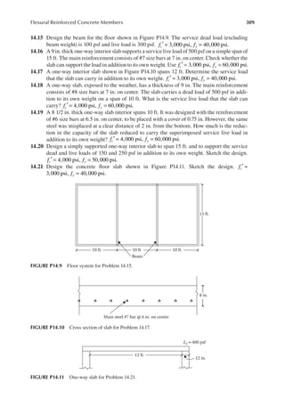
328. 310 Principles of Structural Design
14.22 Design the slab of the loor system in Problem 14.15. f f
c y
3,000 psi, 40,000 psi.
′ = =
[Hint: The slab weight is included in the service dead load.]
14.23 For Problem 14.15, design the thinnest slab so that the strain in steel is not less than 0.005.
f f
c y
3,000 psi, 40,000 psi.
′ = =
14.24 Design a balcony slab exposed to the weather. The cantilevered span is 8 ft. and the
service live load is 100 psf. Use the reinforcement of #5 size bars. Sketch the design.
f f
c y
4,000 psi, 60,000 psi.
′ = =
[Hint: Reinforcement is placed on top. For the thickness of slab, in addition to the provi-
sion of main steel and shrinkage steel, at least 3 in. of depth (cover) should exist over and
below the steel.]

329. 311
15 Doubly and T Reinforced
Concrete Beams
DOUBLY REINFORCED CONCRETE BEAMS
Sometimes the aesthetics or architectural considerations necessitate a small beam section that is not
adequate to resist the moment imposed on the beam. In such cases, the additional moment capacity
could be achieved by adding more steel on both the compression and tensile sides of the beam. Such
sections are known as doubly reinforced beams. The compression steel also makes beams more
ductile and more effective in reducing delections.
The moment capacity of doubly reinforced beams is assumed to comprise two parts as shown
in Figure 15.1. One part is due to the compression concrete and tensile steel, shown in Figure 15.1b
as described in Chapter 14. The other part is due to the compression steel and the additional tensile
steel shown in Figure 15.1c.
Thus,
1 2
A A A
s s s
= +
1 2
M M M
u u u
= +
2
1 1
M A f d
a
u s y
= φ −






and
= φ − ′
M A f d d
u s y ( )
2 2
The combined capacity is given by
2
( )
1 2
M A f d
a
A f d d
u s y s y
= φ −





 + φ − ′ (15.1)
where
φ is resistance factor
d is effective depth
As is area of steel on the tensile side of the beam; 1 2
A A A
s s s
= +
As
′ is area of steel on the compression side of the beam
The compression steel area As
′ depends on the compression stress level fs′, which can be the yield
stress fy or less. The value of fs′ is decided by the strain in concrete at compression steel level, which
in turn depends upon the location of the neutral axis.
From the strain diagram, when concrete attains the optimal strain level at the top as shown in
Figure 15.2,
0.003 –
c d
c
s
( )
′
ε =
′
(15.2)

330. 312 Principles of Structural Design
0.003 ( – )
d c
c
t
ε = (15.3)
1. When f E
s y
′
ε ≥ , the compression steel has yielded, f f
s y
′ = , and from the forces shown in
Figure 15.1c,
2
A A
s s
= ′ (15.4)
2. When ′
ε < f E
s y , the compression steel has not yielded, f E
s s
′ = ′
ε , and again from the forces
shown in Figure 15.1c,
2
A
A f
f
s
s s
y
=
′ ′
(15.5)
3. When 0.005
ε ≥
t , φ = 0.9.
4. When 0.005
ε <
t , compute φ from Equation 14.13.
To ascertain the value of neutral axis, c, the tensile strength of the beam is equated with the
compression strength. Thus, from Figure 15.1
Tensile force Compression force
0.85
0.85
1 2
1 2
( )
=
+ = ′ + ′ ′
+ = ′ + ′ ′
ε
A f A f f ab A f
A A f f ab A E
s y s y c s s
s s y c s s
Substituting a = β1c from Equation 14.3, ε′s from Equation 15.2 and E = 29000 ksi
0.003
dʹ
d–c
c
εt
εʹs
FIGURE 15.2 Strain diagram of concrete.
Aʹ
s Aʹ
s
As
(a) (b) (c)
As1 As2
dʹ
fy As1
As2 fy
Aʹ
s f ʹ
s
+
=
a
0.85 fʹ
c
d –dʹ
d
b
FIGURE 15.1 Moment capacity of doubly reinforced beam.

331. 313
Doubly and T Reinforced Concrete Beams
0.85
( – )
0.003 29,000
1 ( )( )
= ′β + ′
′
A f f cb A
c d
c
s y c s (15.6)
where β1 is given in Equation 14.4, and the others terms are explained in Figure 15.1
ANALYSIS OF DOUBLY REINFORCED BEAMS
A summary of the steps for analysis of a doubly reinforced beam is presented below:
1. From Equation 15.6, determine c; and from Equation 14.3, compute a.
2. From Equation 15.2 compute s
′
ε . If ε′s < fy / E, that is the compression steel has not yielded,
use Equation 15.5 to determine As2, otherwise use Equation 15.4 to determine As2.
3. From Equation 15.3, compute t
ε and from that determine φ as stated in step 3 and 4 of
previous section.
4. Compute the moment capacity from Equation 15.1.
Example 15.1
DeterminethemomentcapacityofthebeamshowninFigure15.3.Use fc′ = 3,000 psi,fy =60,000psi.
SOLUTION
1. From Equation 15.6
A f f cb A
c d
c
s y c s ( )( )
= ′β + ′
′
0.85
( – )
0.003 29,000
1
c
c
c
6.24 60 0.85 3 0.85 14 2
( – 2.5)
0.003 29,000
( ) ( )( ) ( ) ( )( )
= +
c
c
c
c c c
c c
c c
c ( )
( )
( ) ( )
= +
= +
− =
=
=
+ ± +
=
374.4 30.345
174 – 2.5
374.4 30.345 174 – 435
30.345 – 200.4 435 0
– 6.60 – 14.335 0
6.60 6.60 4 14.335
2
8.32in. positive value
2
2
2
2
)
(
= β = =
0.85 8.32 7.07 in.
1
a c
14 in.
2 # 9
4 # 11
26 in.
2½ in.
2½ in.
FIGURE 15.3 Beam section of Example 15.1.

332. 314 Principles of Structural Design
2. From Equation 15.2
c d
c
s
( )
( )
′
ε =
′
= =
0.003 –
0.003 8.32 – 2.5
8.32
0.0021
f
E
y
= =
60
29,000
0.0021
Since f E
s y
′
ε = , the compression steel has yielded.
f f
s y
′ = = 60 ksi
A A
s s
= ′ = 2in.
2
2
As = =
6.24 – 2 4.24 in.
1
2
3. From Equation 15.3
d c
c
t
0.003 ( – )
0.003 23.5 – 8.32
8.32
0.0055
( )
ε =
= =
Since t 0.005
ε > , φ = 0.9.
4. Moment capacity, from Equation 15.1
M A f d
a
A f d d
u s y s y ( )
( )( ) ( )( )( )
= φ −





 + φ − ′
= −





 + −
=
2
0.9 4.24 60 23.5
7.07
2
0.9 2 60 23.5 2.5
6839.19 in.-k or 569.9 ft.-k
1 2
Example 15.2
Determine the moment capacity of the beam shown in Figure 15.4. Use fc′ = 4,000 psi, fy = 60,000 psi.
14 in.
2 # 8
4 # 11
24 in.
3 in.
3 in.
FIGURE 15.4 Beam section of Example 15.2.

333. 315
Doubly and T Reinforced Concrete Beams
SOLUTION
1. From Equation 15.6
A f f cb A
c d
c
s y c s ( )( )
= ′β + ′
′)
0.85
( –
0.003 29,000
1
6.24 60 0.85 4 0.85 14 1
.58
( – 3)
0.003 29,000
c
c
c
( ) ( )( ) ( ) ( )( )
= +
c
c
c c c
c c
c c
c ( )
( )
( ) ( )
= +
= +
− =
=
=
+ ± +
=
374.4 40.46 137.46
– 3
c
374.4 40.46 137.46 – 412.38
40.46 – 236.94 412.38 0
– 5.856 – 10.19 0
5.856 5.856 4 10.19
2
7.26 in. positive value
2
2
2
2
a c 0.85 7.26 6.17 in.
1 ( )
= β = =
2. From Equation 15.2
c d
c
s
( )
( )
′
ε =
′
= =
0.003
–
0.003 7.26 – 3
7.26
0.0018
f
E
y
= =
60
29,000
0.0021
Since f E
s y
′
ε < , the compression steel has not yielded.
f E
s s
′
ε ( )
′ = = =
0.0018 29,000 52.20 ksi
From Equation 15.5
A
A f
f
s
s s
y
( )
=
′ ′
= =
1
.58 52.20
60
1
.375in.
2
2
As = =
6.24 – 1
.375 4.865in.
1
2
3. From Equation 15.3
d c
c
t
0.003 ( – )
0.003 24 – 7.26
7.26
0.0069
( )
ε =
= =
Since t 0.005
>
ε , φ = 0.9.
4. Moment capacity, from Equation 15.1
M A f d
a
A f d d
u s y s y ( )
( )( ) ( )( )( )
= φ −





 + φ − ′
= −





 + −
=
2
0.9 4.865 60 24
6.17
2
0.9 1
.375 60 24 3
7053.9 in.-k or 587.8 ft.-k
1 2

334. 316 Principles of Structural Design
DESIGN OF DOUBLY REINFORCED BEAMS
A summary of the steps to design a doubly reinforced beam is presented below:
1. Determine the factored moment Mu due to applied loads.
2. Ascertain ρ corresponding to 0.005
t
ε = from Appendix D, Table D.11 and K from
Appendix D, Tables D.4 through D.10 and also determine As1 = ρbd.
3. Compute 1
2
M bd K
u = φ , assuming φ = 0.9.
4. Compute Mu2 = Mu – Mu1.
5. Compute (1)
0.85
1
a
A f
f b
s y
c
=
′
and (2) c a
= β
/ 1 .
6. Compute s
′
ε from Equation 15.2.
When f E
s y
′
ε ≥ , the compression steel has yielded, f f
s y
′ = .
When f E
s y
′
ε < , the compression steel has not yielded, f E
s s
′
ε
′ = .
7. Compute
2
A
M
f d d
s
u
s ( )
′ =
φ ′ − ′
8. Compute
2
A
A f
f
s
s s
y
=
′ ′
If the amount of compression steel As
′ and tensile steel As are selected exactly as computed, t
ε will
be 0.005, that is, the tension-controlled condition prevails. However, selecting different amounts of
steel may change this condition resulting in a reduced value of φ of less than 0.9. Technically, after
the amounts of steel are selected, it converts to a problem of analysis as described in the previous
section to conirm that the resisting moment capacity is adequate for the applied bending moment.
Example 15.3
A simply supported beam of span 30 ft. is subjected to a dead load of 2.4 k/ft. and a live load
of 3.55 k/ft. From architectural consideration, the beam dimensions are ixed as shown in Figure
15.5. Design the beam. Use fc′ = 4,000 psi and fy = 60,000 psi.
28 in.
3 in.
15 in.
FIGURE 15.5 Size of beam for Example 15.3.

335. 317
Doubly and T Reinforced Concrete Beams
SOLUTION
1. = × × × =
Weight ofbeam/ft.
31
12
15
12
1 150 484 lb/ft. or 0.484 k/ft.
wu 1
.2 2.4 0.484 1
.6 3.55 9.141k/ft.
) )
( (
= + + =
M
wL
u
( )
= = =
8
9.41 30
8
1028.4 ft.-k
2 2
2. From Appendix D, Table D.11, ρ = 0.0181.
From Appendix D, Table D.9, 0.911ksi
K = .
A bd
s 0.0181 15 28 7.6 in.
1
2
( )( )( )
=ρ = =
3. M bd K
u ( )( )( ) ( )
= φ = =
0.9 15 28 0.911 9642in.-k or 803.5 ft.-k
1
2 2
4. M M M
u u u
= − = − =
1028.4 803.5 224.9 ft.-k or 2698.8 in.-k
2 1
5. a
A f
f b
s y
c
( )
( )( )
=
′
= =
0.85
760 60
0.85 4 15
8.94 in.
1
8.94
0.85
10.52in.
1
c
a
=
β
= =
6. c d
c
s
( )
( )
′
ε =
′
= =
0.003
–
0.003 10.52 – 3
10.52
0.0021
f
E
y
= =
60
29,000
0.0021
Since f E
s y
′
ε = , the compression steel has yielded.
f f
s y
′= =60 ksi
7. A
M
f d d
A
s
u
s
s
( ) ( )( )
′ =
φ ′ − ′
=
−
= ′ =
2698.8
0.9 60 28 3
2.0 in. ; Use 2 bars of#9, 2in.
2 2 2
8. A
A f
f
s
s s
y
( )
=
′ ′
= =
2.0 60
60
2in.
2
2
A A
s s
= + = =
7.6 2.0 9.6 in. ; Use 8 bars of#10, 10.2in.
2 2 (two layers)
MONOLITHIC SLAB AND BEAM (T BEAMS)
The concrete loor systems generally consist of slabs and beams that are monolithically cast together.
In such cases the slab acts as a part of the beam, resulting in a T-shaped beam section as shown in
Figure 15.6. The slab portion is called a lange and the portion below the slab is called a web. The
slab spans from beam to beam. But, the American Concrete Institute (ACI) code deines a limited
width that can be considered as a part of the beam. According to ACI this effective lange width
should be the smallest of the following three values:*
1. bf = one-fourth of the span (15.7a)
2. bf = bw + 16 hf (15.7b)
3. bf = center to center spacing of beams (15.7c)
A T beam has ive relevant dimensions: (1) lange width, bf; (2) lange thickness, hf; (3) width of
web or stem, bw; (4) effective depth of beam, d; and (5) tensile steel area, As.
* For an L-shaped beam, the overhang portion of the lange should be the smallest of (1) one-twelfth of the span length;
(2) six times the slab thickness, hf; and (3) one-half of the clear distance between beams.

336. 318 Principles of Structural Design
In analysis type of problems, all ive of these parameters are known and the objective is to deter-
mine the design capacity of the beam. In the design of T beams, the lange is designed separately as
a slab spanning between the beams (webs) according to the procedure described for one-way slabs
in Chapter 14. The effective width of the lange is ascertained according to Equation 15.7. The size
of the web is ixed to satisfy the shear capacity or other architectural requirements. Thus the values
of bf, hf, bw, and d are preselected and a design consists of computing of the area of tensile steel.
Under a positive bending moment, the concrete on the lange side resists compression and the
steel in the web resists tension. Depending on the thickness of the lange, the compression stress
block might fully conine within the lange or it might fully cover the lange thickness and further
extend into the web. Mostly the former condition exists.
In the irst case a T beam acts like a rectangular beam of width bf because all the concrete area
below the compression stress block is considered to be cracked, and thus any shape of concrete
below this compression stress block does not matter.
The minimum steel requirements as specified by Equations 14.11 and 14.12 apply to T
beams also.
ANALYSIS OF T BEAMS
1. Determine the effective lange width, bf from Equation 15.7.
2. Check for minimum steel using Equations 14.11 and 14.12 using web width bw for beam
width.
3. Determine the area of the compression block, Ac:
0.85
A
A f
f
c
s y
c
=
′
(15.8)
4. In most cases, A b h
c f f
≤ , that is, the compression stress block lies within the lange. In such
cases the depth of the stress block is given by
a
A
b
c
f
= (15.9)
and the centroid of the compression block from the top is given by
y a
=
2
(15.10)
Slab
hf
bf
Effective flange width
Beam spacing
Flange
Web or stem
Web width
As
bw
d
FIGURE 15.6 T beam comprising slab and supporting beam of a loor system.

337. 319
Doubly and T Reinforced Concrete Beams
5. When A b h
c f f
> , the compression stress block extends into the web to an extent Ac
exceeding the lange area b h
f f . The centroid is determined for the area of the lange and
the area extending into web as demonstrated in Example 15.4.
6. Determine (1) c a
= β
/ 1, where β1 is given in Equation 14.4; (2) 0.0003( )/
d c c
t
ε = −
and (3) Z = d – y.
7. If 0.005
t
ε < , adjust φ by Equation 14.13.
8. Calculate the moment capacity:
M A f Z
n s y
φ = φ
Example 15.4
Determine the moment capacity of the T beam spanning 20 ft., as shown in Figure 15.7. Use
fc 3,000 psi
′ = and fy = 60,000 psi.
SOLUTION
1. Effective lange width, bf
a. span
4
20 12
4
60 in.
=
×
=
b. bw + 16hf = 11 + 16(3) = 59 in.
c. Beam spacing = 3 × 12 = 36 in. ← Controls
2. Minimum steel
a. f b d
f
c w
y
( )( )
′
= =
3 3 3,000 11 24
60,000
0.723in.2
b. b d
f
w
y
( )( )
= = <
200 200 11 24
60,000
0.88 in. 6.35in.
2 2
OK
3. Area of compression block
A
A f
f
c
s y
c
( )( )
( )( )
=
′
= =
0.85
6.35 60,000
0.85 3,000
149.41in.2
b h
f f ( )( )
= =
36 3 108 in.2
Since 149.41 > 108, the stress block extends into web by a distance a1 below the lange.
4. a
A b h
b
c f f
w
=
−
=
−
=
149.41 108
11
3.76 in.
1
2
= + =
3 3.76 6.76 in.
a
5–#10 As= 6.35 in.2
hf = 3 in.
3 ft.
11 in.
24 in.
FIGURE 15.7 T beam dimensions for Example 15.4.

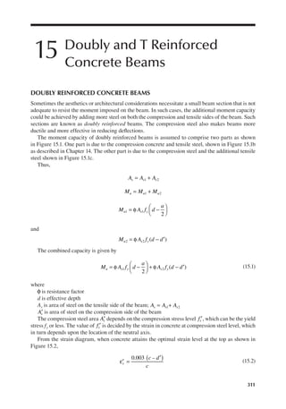
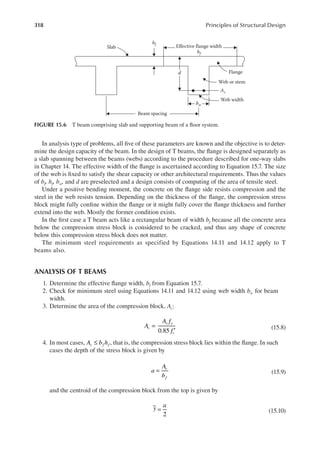
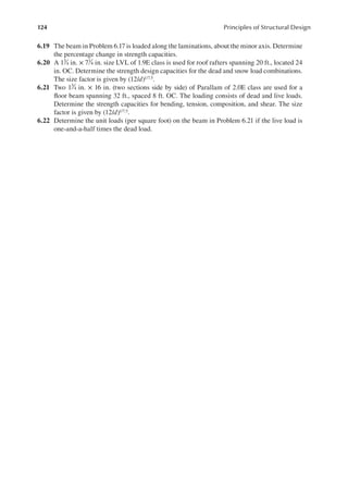
338. 320 Principles of Structural Design
5. In Figure 15.8, the centroid of the compression block from the top:
y
( )
[ ]
=
× × + × × +

 
 =
36 3 1
.5 11 3.76 3 3.76/2
149.41
2.435in.
6. = =
6.76
0.85
7.95in.
c
t
( )
ε =
−
= > φ =
0.003 24 7.95
7.95
0.0061 0.005, hence 0.9
24 2.435 21
.565
Z d y
= − = − = in.
7. Moment capacity
M A f Z
n s y ( )( )( )
φ = φ = =
0.9 6.35 60 21
.565 7394.64 in.-k or 616.2 ft.-k
DESIGN OF T BEAMS
As stated earlier, design consists of determining only the tensile steel area of a T beam. This process
is the reverse of the analysis. The steps are as follows:
1. Compute the factored design moment including the dead load.
2. Determine the effective lange width, bf, from Equation 15.7.
3. Adopt the effective depth d = h – 3 when the overall depth h is given. Assume the moment
arm Z to be the larger of the following:
(1) 0.9d or (2) (d – hf/2).
4. Calculate the steel area:
, for initial value of 0.9
A
M
f Z
s
u
y
=
φ
φ =
5. Calculate the area of the compression block, Ac:
0.85
A
A f
f
c
s y
c
=
′
(15.8)
6. Determine the depth of the stress block, a.
In most cases, A b h
c f f
≤ , that is, the compression stress block lies within the lange. In such
cases the depth of the stress block is given by
c
N A
bf = 36 in.
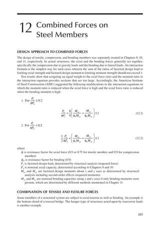
hf = 3 in.
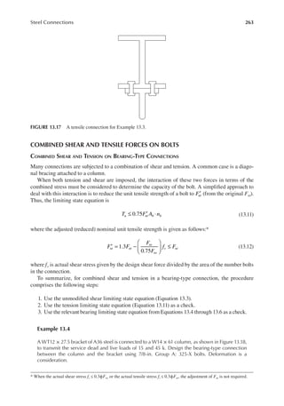
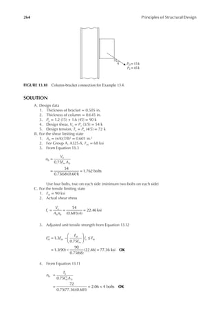
Ac = 149.41 in.
2
11 in.
5 #10
a
a1
FIGURE 15.8 Compression stress block for Example 15.4.

339. 321
Doubly and T Reinforced Concrete Beams
a
A
b
c
f
= (15.9)
and the centroid of the compression block from the top is given by
y
a
=
2
(15.10)
When A b h
c f f
> , the compression stress block extends into web to the extent Ac exceeding
the lange area bfhf. The centroid is determined for the areas in the lange and web as shown
in Example 15.4.
7. Determine (1) = β
c a/ 1, where β1 is given in Equation 14.4; and (2)
0.003( – )
d c
c
t
ε = .
8. If 0.05
t
ε < , adjust φ by Equation 14.13 and recalculate the steel area from step 4.
9. Compute the revised moment arm:
Z d a
= −
If the computed Z is appreciably different than the assumed Z of step 3, repeat steps 4
through 6, until the value of Z stabilizes.
10. Make a selection of steel for the inal value of As computed.
11. Check for minimum steel by Equations 14.11 and 14.12 or Appendix D, Table D.11.
Example 15.5
Design a T beam for the loor system spanning 20 ft., as shown in Figure 15.9. The moments due
to dead load (including beam weight) and live load are 200 ft.-k and 400 ft.-k, respectively. Use
fc =
′
3,000 psi and fy = 60,000 psi.
SOLUTION
1. Factored design moment = 1.2(200) = 1.6(400) = 960 ft.-k or 11,520 in.-k.
2. Effective lange width, bf
a.
span
4
20 12
4
60 in. Controls
=
×
= ←
b. B h
w f ( )
+ = + =
16 15 16 3 63in.
c. Beam spacing 6 12 72in.
= × =
3. Moment arm
0.9 0.9 24 21
.6 in.
Z d ( )
= = =
Z d
hf
= − = − = ←
2
24
3
2
22.5in. Controls
15 in.
hf = 3 in.
6 ft.
FIGURE 15.9 T beam section for Example 15.5.

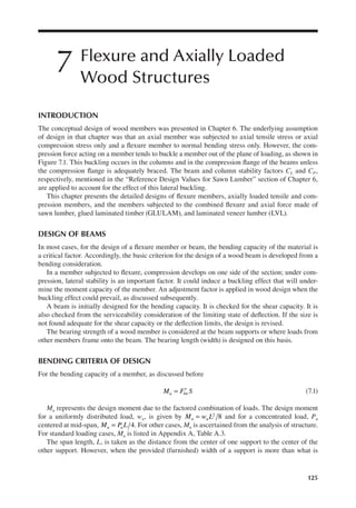
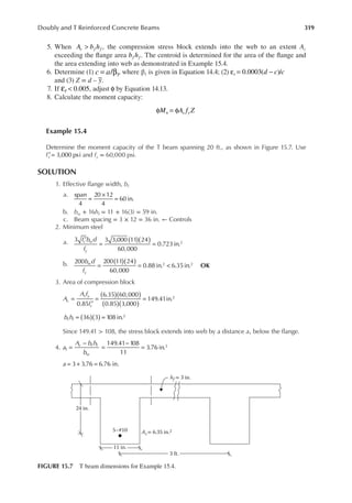
340. 322 Principles of Structural Design
4. Steel area
A
M
f Z
s
u
y ( )( )( )
=
φ
= =
11,520
0.9 60 22.5
9.48 in.2
5. Area of compression block
A
A f
f
c
s y
c
( )( )
( )( )
=
′
= =
0.85
9.48 60,000
0.85 3,000
223.06 in.2
b h
f f ( )( )
= =
60 3 180 in.2
Since 223.06 > 180, the stress block extends into the web by a distance a1 below the lange
6. a
A b h
b
c f f
w
=
−
=
−
=
223.06 80
15
2.87 in.
1
2
= + =
3 2.87 5.87 in.
a
7. In Figure 15.10, the centroid of the compression block from the top
y
[ ]
[ ]
=
× × + × 2.87 × (3 + 2.87/2)
=
60 3 1
.5 15
223.06
2.066 in.
8.
5.87
0.85
6.91in.
c = =
t
( )
ε =
−
= > φ =
0.003 24 6.91
6.91
0.0074 0.005, hence 0.9
24 2.066 21
.93in.
Z d y
= − = − =
9. Revised steel area
A
M
f Z
s
u
y ( )( )( )
=
φ
= =
11,520
0.9 60 21
.93
9.73in.2
Select 10 bars of #9, As = 10 in.2 in two layers.
The steel area could be reined further by a small margin by repeating steps 5 through 9.
10. Minimum steel
1.
f b d
f
c w
y
( )( )
′
= =
3 3 3,000 15 24
60,000
0.99 in.2
2.
b d
f
w
y
( )( )
= = <
200 200 15 24
60,000
1
.20 in. 9.73 in.
2 2
OK
24 in.
6.91 in. 5.87 in.
N A
60 in.
3 in.
15 in.
FIGURE 15.10 Compression stress block for Example 15.5.

341. 323
Doubly and T Reinforced Concrete Beams
PROBLEMS
15.1 Determine the design strength of the beam shown in Figure P15.1. Use 4,000 psi
fc′ = and
60,000 psi
fy = .
15.2 Determine the design strength of the beam shown in Figure P15.2. Use 3,000 psi
fc′ = and
60,000 psi
fy = .
15.3 Determine the design strength of the beam shown in Figure P15.3. Use 4,000 psi
fc′ = and
60,000 psi
fy = .
15.4 Determine the design strength of the beam shown in Figure P15.4. Use 5,000 psi
fc′ = and
60,000 psi
fy = .
15.5 A beam of the dimensions shown in Figure P15.5 is subjected to a dead load of
690 lb/ft. and a live load of 1500 lb/ft. It has a simple span of 35 ft. Design the beam. Use
4,000 psi
fc′ = and 60,000 psi
fy = .
15.6 Design a beam to resist the moment due to service dead load of 150 ft.-k (including weight)
and the moment due to service live load of 160 ft.-k. The beam width is limited to 11 in.
and the effective depth is limited to 20 in. The compression steel is 3 in. from the top. Use
3,000 psi
fc′ = and 60,000 psi
fy = .
3 # 6
5 # 11
16.5 in.
2½ in.
2½ in.
23 in.
FIGURE P15.1 Beam section for Problem 15.1.
2 # 10
4 # 11
11 in.
2½ in.
25 in.
4 in.
FIGURE P15.2 Beam section for Problem 15.2.
4 # 7
4 # 11
15 in.
2½ in.
20 in.
3 in.
FIGURE P15.3 Beam section for Problem 15.3.

342. 324 Principles of Structural Design
15.7 Design a beam to resist the total factored moment (including weight) of 1,000 ft.-k. The
dimensions are as shown in Figure P15.6. Use 4,000 psi
fc′ = and fy = 50,000 psi.
15.8 Determine the design moment capacity of the T beam shown in Figure P15.7, spanning
25 ft. Use 4,000 psi
fc′ = and 60,000 psi
fy = .
15.9 Determine the design capacity of the beam in Problem 15.8. The slab thickness is 3 in. and
the center to center spacing of beams is 3 ft. Use 3,000 psi
fc′ = and 60,000 psi
fy = .
15.10 Design a T beam for the loor system shown in Figure P15.8. The live load is 200 psf
and the dead load is 60 psf excluding the weight of the beam. The slab thickness is 4 in.,
the effective depth is 25 in., and the width of the web is 15 in. Use 3,000 psi
fc′ = and
60,000 psi
fy = .
15.11 Design the T beam shown in Figure P15.9 that spans 25 ft. The moment due to service
dead load is 200 ft.-k (including beam weight) and due to service live load is 400 ft.-k. Use
4,000 psi
fc′ = and 60,000 psi
fy = .
14 in.
3 in.
25 in.
4 in.
FIGURE P15.6 Beam dimensions for Problem 15.7.
2 # 8
3 # 11
11 in.
2½ in.
21 in.
3 in.
FIGURE P15.4 Beam section for Problem 15.4.
15 in.
4 in.
16 in.
4 in.
FIGURE P15.5 Beam dimensions for Problem 15.5.

343. 325
Doubly and T Reinforced Concrete Beams
6 # 9
hf = 4 in.
5 ft.
12 in.
25 in.
FIGURE P15.7 T beam section for Problem 15.8.
40 ft.
T beam
@ 5 ft. center
60 ft.
FIGURE P15.8 Floor system for Problem 15.10.
3 in.
4 ft.
12 in.
24 in.
FIGURE P15.9 T beam section for Problem 15.11.

345. 327
16 Shear and Torsion in
Reinforced Concrete
STRESS DISTRIBUTION IN BEAM
The transverse loads on a beam segment cause a bending moment and a shear force that vary across
the beam cross section and along the beam length. At point (1) in a beam shown in Figure 16.1,
these contribute to the bending (lexure) stress and the shear stress, respectively, expressed as
follows:
f
My
I
b = (16.1a)
and
f
VQ
Ib
v = (16.1b)
where
M is bending moment at a horizontal distance x from the support
y is vertical distance of point (1) from the neutral axis
I is moment of inertia of the section
V is shear force at x
Q is moment taken at the neutral axis of the cross-sectional area of the beam above point (1)
b is width of section at (1)
The distribution of these stresses is shown in Figure 16.2. At any point (2) on the neutral axis, the
bending stress is zero and the shear stress is maximum (for a rectangular section). On a small ele-
ment at point (2), the vertical shear stresses act on the two faces balancing each other, as shown in
Figure 16.2. According to the laws of mechanics, the complementary shear stresses of equal mag-
nitude and opposite sign act on the horizontal faces as shown, so as not to cause any rotation to the
element.
If we consider a free-body diagram along the diagonal a–b, as shown in Figure 16.3, and resolve
the forces (shear stress times area) parallel and perpendicular to the plane a–b, the parallel force
will cancel and the total perpendicular force acting in tension will be 1.414fvA. Dividing by the
area 1.41A along a–b, the tensile stress acting on plane a–b will be fv. Similarly, if we consider a
free-body diagram along the diagonal c–d, as shown in Figure 16.4, the total compression stress
on the plane c–d will be fv. Thus, the planes a–b and c–d are subjected to tensile stress and com-
pression stress, respectively, which has a magnitude equal to the shear stress on the horizontal and
vertical faces. These stresses on the planes a–b and c–d are the principal stresses (since they are
not accompanied by any shear stress). The concrete is strong in compression but weak in tension.
Thus, the stress on plane a–b, known as the diagonal tension, is of great signiicance. It is not the
direct shear strength of concrete but the shear-induced diagonal tension that is considered in the
analysis and design of concrete beams.

346. 328 Principles of Structural Design
d
a
b
c
fv
fv
fv
fv
FIGURE 16.2 Shear stresses at neutral axis.
fv • A
fv • A
0.707fv • A
0.707fv • A
Force component
Plane in tension
0
.
7
0
7
f
v
•
A
0
.
7
0
7
f
v
•
A
a
45°
b
A
r
e
a
=
1
.
4
1
4
A
AreaA
Area
A
FIGURE 16.3 Free body diagram along plane a–b of element of Figure 16.2.
fv • A
c
d
0.707fv • A
0.707fv • A
0
.
7
0
7
f
v
•
A
0
.
7
0
7
f
v
•
A
fv • A
Plane in compression
FIGURE 16.4 Free body diagram along plane c–d of element of Figure 16.2.
x
b fb fv
y 1
2
FIGURE 16.1 Flexure and shear stresses on transverse loaded beam.

347. 329
Shear and Torsion in Reinforced Concrete
DIAGONAL CRACKING OF CONCRETE
There is a tendency for concrete to crack along the plane subjected to tension when the level of stress
exceeds a certain value. The cracks will form near the mid-depth where the shear stress (includ-
ing the diagonal tension) is maximum and will move in a diagonal path to the tensile surface, as
shown in Figure 16.5. These are known as the web-shear cracks. These are nearer to the support
where shear is high. In a region where the moment is higher than the cracking moment capacity, the
vertical lexure cracks will appear irst and the diagonal shear cracks will develop as an extension
to the lexure cracks. Such cracks are known as the lexure-shear cracks. These are more frequent
in beams. The longitudinal (tensile) reinforcement does not prevent shear cracks but it restrains the
cracks from widening up.
After a crack develops, the shear resistance along the cracked plane is provided by the following
factors:
1. Shear resistance provided by the uncracked section above the crack, Vcz. This is about
20%–40% of the total shear resistance of the cracked section.
2. Friction developed due to interlocking of the aggregates on opposite sides of the crack, Va.
This is about 30%–50% of the total.
3. Frictional resistance between concrete and longitudinal (main) reinforcement called the
dowel action, Vd. This is about 15%–25% of the total.
In a deep beam, some tie–arch action is achieved by the longitudinal bars acting as a tie and the
uncracked concrete above and to the sides of the crack acting as an arch.
Once the applied shear force exceeds the shear resistance offered by the above three factors in
a cracked section, the beam will fail suddenly unless a reinforcement known as the web or shear
reinforcement is provided to prevent the further opening up of the crack. It should be understood
that the web reinforcement does not prevent the diagonal cracks that will happen at almost the same
loads with or without a web reinforcement. It is only after a crack develops that the tension that was
previously held by the concrete is transferred to the web reinforcement.
STRENGTH OF WEB (SHEAR) REINFORCED BEAM
As stated above, the web reinforcement handles the tension that cannot be sustained by a diagonally
cracked section. The actual behavior of web reinforcement is not clearly understood in spite of
many theories presented. The truss analogy is the classic theory, which is very simple and widely
used. The theory assumes that a reinforced concrete beam with web reinforcement behaves like a
truss. A concrete beam with vertical web reinforcement in a diagonally cracked section is shown
in Figure 16.6. The truss members shown by dotted lines are superimposed in Figure 16.6. The
analogy between the beam and the truss members is as shown in Table 16.1.
Vd
Va
Vcz
FIGURE 16.5 Shear resistance of cracked concrete.

348. 330 Principles of Structural Design
According to the above concept, the web reinforcement represents the tensile member. According
to the truss analogy theory, the entire applied shear force that induces the diagonal tension is
resisted only by the web reinforcement. But observations have shown that the tensile stress in the
web reinforcement is much smaller than the tension produced by the entire shear force. Accordingly,
the truss analogy theory was modiied to consider that the applied shear force is resisted by two
components: the web reinforcement and the cracked concrete section. Thus,
V V V
n c s
= + (16.2)
Including a capacity reduction factor, ϕ,
V V
u n
≤ φ (16.3)
For the limiting condition
V V V
u c s
= φ + φ (16.4)
where
Vn is nominal shear strength
Vu is factored design shear force
Vc is shear contribution of concrete
Vs is shear contribution of web reinforcement
ϕ is capacity reduction factor for shear = 0.75 (Table 14.1)
Equation 16.4 serves as a design basis for web (shear) reinforcement.
Tensile members
of truss= web reinforcement
Compression members
of truss= concrete
between cracks
Concrete
between cracks
Stirrups
Diagonal crack
45°
Horizontal compression
members of truss
(top chord)= flexure
compression concrete
C
T
Horizontal compression
members of truss
(bottom chord)=
longitudinal
reinforcement
FIGURE 16.6 Truss analogy of beam.
TABLE 16.1
Beam–Truss Analogy
Truss Beam
Horizontal tensile member (bottom chord) Longitudinal reinforcement
Horizontal compression member (top chord) Flexure compression concrete
Vertical tensile members Web reinforcement
Diagonal compression members Web concrete between the cracks in the compression zone

349. 331
Shear and Torsion in Reinforced Concrete
SHEAR CONTRIBUTION OF CONCRETE
Concrete (with lexure reinforcement but without web reinforcement) does not contribute in resist-
ing the diagonal tension once the diagonal crack is formed. Therefore, the shear stress in concrete at
the time of diagonal cracking can be assumed to be the ultimate strength of concrete in shear. Many
empirical relations have been suggested for the shear strength. The American Concrete Institute
(ACI) has suggested the following relation:
V f bd
c c
= λ ′
2 (16.5)
The expression λ was introduced in the ACI 2008 code, to account for lightweight concrete; for nor-
mal weight concrete λ = 1. An alternative, much more complicated expression has been proposed
by the ACI, which is a function of the longitudinal reinforcement, bending moment, and shear force
at various points of beam.
SHEAR CONTRIBUTION OF WEB REINFORCEMENT
The web reinforcement takes a form of stirrups that run along the face of a beam. The stirrups
enclose the longitudinal reinforcement. The common types of stirrups, as shown in Figure 16.7, are
shaped or shaped and are arranged vertically or diagonally. When a signiicant amount of tor-
sion is present, the closed stirrups are used, as shown in Figure 16.7c.
The strength of a stirrup of area Av is fy Av. If n number of stirrups cross a diagonal crack, then
the shear strength by stirrups across a diagonal will be
V f A n
s y v
= (16.6)
In a 45° diagonal crack, the horizontal length of crack equals the effective depth d, as shown in
Figure 16.8. For stirrups spaced s on center, n = d/s. Substituting this in Equation 16.6, we have
V f A
d
s
s y v
= (16.7)
(a) (b) (c)
FIGURE 16.7 Types of stirrups: (a) open stirrup, (b) double stirrup, (c) closed stirrup.
s
d
45°
d
FIGURE 16.8 Vertical stirrup in a diagonal crack.

350. 332 Principles of Structural Design
where
Av is area of stirrups
s is spacing of stirrups
For a shaped stirrup, Av is twice the area of the bar and for a stirrup, Av is four times the bar
area.
When the stirrups are inclined at 45°, the shear force component along the diagonal will match
the stirrups (web reinforcement) strength, or
V f A
d
s
s y v
= 1.414 (16.8)
Equations 16.7 and 16.8 can be expressed as a single relation:
V f A
d
s
s y v
= α (16.9)
where α = 1 for the vertical stirrups, and 1.414 for the inclined stirrups.
SPECIFICATIONS FOR WEB (SHEAR) REINFORCEMENT
The requirements of ACI 318-11 for web reinforcement are summarized below:
1. According to Equation 16.4, when Vu ≤ ϕVc, no web reinforcement is necessary. However,
the ACI code requires that a minimum web reinforcement should be provided when Vu
exceeds 1/2ϕVc, except for slabs, shallow beams (≤10 in.), and footing.
2. Minimum steel: When web reinforcement is provided, its amount should fall between the
speciied lower and upper limits. The reinforcing should not be so low as to make the web
reinforcement steel yield as soon as a diagonal crack develops. The minimum web rein-
forcement area should be the higher of the following two values:
( )
0.75
=
′
A
f bs
f
v min
c
y
(16.10)
or
( )
50
=
A
bs
f
v min
y
(16.11)
3. Maximum steel: The maximum limit of web reinforcement is set because the concrete will
eventually disintegrate no matter how much steel is added. The upper limit is
( )
8
=
′
A
f bs
f
a
v max
c
y
(16.12)
4. Stirrup size: The most common stirrup size is #3 bar. Where the value of shear force is
large, #4 bar might be used. The use of larger than #4 size is unusual. For a beam width
of ≤24 in., a single loop stirrup is satisfactory. Up to a width of 48 in. a double loop is
satisfactory.

351. 333
Shear and Torsion in Reinforced Concrete
5. Stirrup spacing
a. Minimum spacing: The vertical stirrups are generally not closer than 4 in. on center.
b. Maximum spacing when V f bd
s c
≤ ′
4 .
The maximum spacing is the smaller of the following:
i.
2
=
s
d
max
ii. smax = 24 in.
iii.
0.75
=
′
s
A f
f b
max
v y
c
(based on Equation 16.10)
iv.
50
=
s
A f
b
max
v y
(based on Equation 16.11)
c. Maximum spacing when 4
V f bd
s c
> ′
The maximum spacing is the smaller of the following:
i.
4
=
s
d
max
ii. smax = 12 in.
iii.
0.75
=
′
s
A f
f b
max
v y
c
(based on Equation 16.10)
iv.
50
=
s
A f
b
max
v y
(based on Equation 16.11)
6. Stirrups pattern: The size of stirrups is held constant while the spacing of stirrups is var-
ied. Generally the shear force decreases from the support toward the middle of the span
indicating that the stirrups spacing can continually increase from the end toward the cen-
ter. From a practical point of view, the stirrups are placed in groups; each group has the
same spacing. Only two to three such groups of the incremental spacing are used within a
pattern. The increment of spacing shall be in a multiple of whole inches perhaps in a mul-
tiple of 3 in. or 4 in.
7. Critical section: For a normal kind of loading where a beam is loaded at the top and there is
no concentrated load applied within a distance d (effective depth) from the support, the section
located at a distance d from the face of the support is called the critical section. The shear
force at the critical section is taken as the design shear value Vu, and the shear force from the
face of the support to the critical section is assumed to be the same as at the critical section.
When the support reaction is in tension at the end region of a beam or the loads are applied at
the bottom (to the tension lange), or it is a bracket (cantilevered) section, no design shear force
reduction is permitted and the critical section is taken at the face of the support itself.
Some designers place their irst stirrup at a distance d from the face of the support while others
place the irst stirrup at one-half of the spacing calculated at the end.
ANALYSIS FOR SHEAR CAPACITY
The process involves the following steps to check for the shear strength of an existing member and
to verify the other code requirements:
1. Compute the concrete shear capacity by Equation 16.5.
2. Compute the web reinforcement shear capacity by Equation 16.9.

352. 334 Principles of Structural Design
3. Determine the total shear capacity by Equation 16.4. This should be more than the applied
factored shear force on the beam.
4. Check for the spacing of the stirrups from the “Speciications for Web (Shear) Reinforcement”
section, step 5.
Example 16.1
Determine the factored shear force permitted on a reinforced concrete beam shown in Figure 16.9.
Check for the web reinforcement spacing. Use ′
fc = 4,000 psi, fy = 60,000 psi.
SOLUTION
A. Concrete shear capacity from Equation 16.5
2
2 1 4000 16 27 54644 lb or 54.64 k
) ) )
( ( (
= λ ′
= =
V f bd
c c
B. Web shear capacity from Equation 16.9
2 0.11 0.22in.2
)
(
= =
Av
V f A
d
s
s y v
1 60,000 0.22
27
12
29,700 lb or 29.7 k
( )( )
= α
=





 =
C. Design shear force from Equation 16.4
V V V
u c s
0.75(54.64) 0.75(29.7) 63.26 k
= φ + φ
= + =
D. Maximum spacing
1. f bd
c
4 /1000 4 4000(16)(27)/1000 109.3k
′ = =
2. Since Vs of 29.7 k < 109.3 k
#3 @
12 in. OC
4-#8
27 in.
16 in.
FIGURE 16.9 Section for Example 16.1.

353. 335
Shear and Torsion in Reinforced Concrete
Maximum spacing is smaller of
a.
d
OK
2
27
2
13.5in. Controls 12in. (as given in Example)
= = ← >
b. 24 in.
c. s
A f
f b
max
v y
c
=
′
= =
0.75
(0.22)(60,000)
(0.75) 4,000(16)
17.4
d. s
A f
b
max
v y
=
= =
50
(0.22)(60,000)
50(16)
16.5in.
DESIGN FOR SHEAR CAPACITY
A summary of the steps to design for web reinforcement is presented below:
1. Based on the factored loads and clear span, draw a shear force, Vu, diagram.
2. Calculate the critical Vu at a distance d from the support and show this on the Vu diagram
as the critical section. When the support reaction is in tension, the shear force at the end is
the critical Vu.
3. Calculate (0.75)2
V f bd
c c
φ = ′ and draw a horizontal line at ϕVc level on the Vu diagram.
The portion of the Vu diagram above this line represents ϕVs, the portion of the shear force
that has to be provided by the web reinforcement or stirrups.
4. Calculate 1/2ϕVc and show it by a point on the Vu diagram. The stirrups are needed from
the support to this point. Below the 1/2ϕVc point on the diagram toward the center, no stir-
rups are needed.
5. Make the tabular computations indicated in steps 5, 6, and 7 for the theoretical stirrups
spacing.
Starting at the critical section, divide the span into a number of segments. Determine
Vu at the beginning of each segment from the slope of the Vu diagram. At each segment,
calculate Vs from the following rearranged Equation 16.4:
( )
V
V V
s
u c
=
− φ
φ
6. Calculate the stirrup spacing for a selected stirrup size at each segment from the following
rearranged Equation 16.9:
( being 1 for vertical stirrup)
s f A
d
V
y v
s
= α α
7. Compute the maximum stirrup spacing from the equations in the “Speciications for Web
(Shear) Reinforcement” section, step 5.

354. 336 Principles of Structural Design
8. Draw a spacing versus distance diagram from step 6. On this diagram, draw a horizontal
line at the maximum spacing of step 7 and a vertical line from step 4 for the cut off limit
stirrup.
9. From the diagram, select a few groups of different spacing and sketch the design.
Example 16.2
The service loads on a reinforced beam are shown in Figure 16.10 along with the designed beam
section. Design the web reinforcement. Use fc
′ = 4,000 psi and fy = 60,000 psi.
SOLUTION
A: Vu diagram
1. Weight of beam = (15/12) × (21/12) × 1 × (150/1000) = 0.33 k/ft.
2. wu = 1.2(3 + 0.33) = 4 k/ft.
3. Pu = 1.6(15) = 24 k
4. M @ B = 0
RA (24) − 4(24)(12) − 24(18) − 24(6) = 0
RA = 72 k
5. Shear force diagram is shown in Figure 16.11
6. Vu diagram for one-half span is shown in Figure 16.12
B. Concrete and steel strengths
1. Critical Vu at a distance, d = 72 − (18/12)(4) = 66 k
2. V f bd
c c
0.75(2) 0.75(2) 4000(15)(18)/1000 25.61k
φ = ′ = =
3. V
φ =
1/2 12.8 k
c
4. Distance from the beam center line to Vc
(1/2)( /slope) 12.8/4 3.2 ft.
φ = =
4-#8
DL=3 k/ft.
(excluding weight)
LL= 15 k
LL= 15 k
A B
6 ft.
12 ft.
6 ft.
15 in.
18 in.
FIGURE 16.10 Load on beam and section for Example 16.2.
72 k
48 k
24 k
48 k
24 k
72 k
6 ft. 12 ft. 6 ft.
FIGURE 16.11 Shear force diagram for Example 16.2.

355. 337
Shear and Torsion in Reinforced Concrete
C. Stirrups design: Use #3 stirrups
Distance versus spacing from the above table are plotted in Figure 16.13.
D. Maximum spacing
1. f bd
c
4 /1000 4 4000(15)(18)/1000 68.3k
′ = =
2. Vs critical of 53.87 k < 68.3 k
3. Maximum spacing is the smaller of
a. = = ←
d
2
18
2
9 in. Controls
b. 24 in.
c. s
A f
f b
max
v y
c
=
′
= =
0.75
(0.22)(60,000)
(0.75) 4,000(15)
18.55
Distance from Support, x, ft. Vu, k s
u c
V
V V
, k
−
− φ
φ
= s f A
d
V
y v
s
, in.
=
1 2 3c 4d
D = 1.5 66a 53.87 4.41
2 64 51.20 4.64
4 56 40.53 5.86
6− 48 29.87 7.96
6+ 24b 0 ∞
a Vu = Vu@end − (slope)(distance) = 72 − 4 (Col. 1).
b Vu = Vu@B in Figure 16.12 − (slope)(distance − 6) = 24 − 4 (Col. 1 − 6).
c (Col. 2 − 25.61)/0.75.
d (60,000/1000)(0.22)(18)/Col. 3.
72 k
66 k
Critical section
Slope 4 k/ft.
Slope 4 k/ft.
No stirrups
needed
d= 1.5ft.
D
C
B
A
ϕVc =25.6 k
48 k
24 k
ϕVc = 12.8 k
1
2
ϕVc
ϕVs
6 ft. 6ft.
3.2 ft.
FIGURE 16.12 Vu diagram for Example 16.2.

356. 338 Principles of Structural Design
d. s
A f
b
max
v y
=
= =
50
(0.22)(60,000)
50(15)
17.6 in.
The smax line is shown in Figure 16.13.
E. Selected spacings
TORSION IN CONCRETE
Torsion occurs when a member is subjected to a twist about its longitudinal axis due to a load act-
ing off center of the longitudinal axis. Such a situation can be seen in a spandrel girder shown in
Figure 16.14.
The moment developed at the end of the beam will produce a torsion in the spandrel girder. A
similar situation develops when a beam supports a member that overhangs across the beam. An
earthquake can cause substantial torsion to the members. The magnitude of torsion can be given by
T Fr
= (16.13)
where
F is force or reaction
r is perpendicular distance of the force from the longitudinal axis
9
∞
Smax =9 in.
8
No stirrups
needed
7
6
Spacing,
in.
5
4
0 1 2 3
Distance from end, ft.
4 5 6 7 8 9
8.8
FIGURE 16.13 Distance-spacing graph for Example 16.2.
Distance Covered, ft. Spacing, in. No. of Stirrups
0–5 4 15
5–6 6 2
6–8.8 9 4

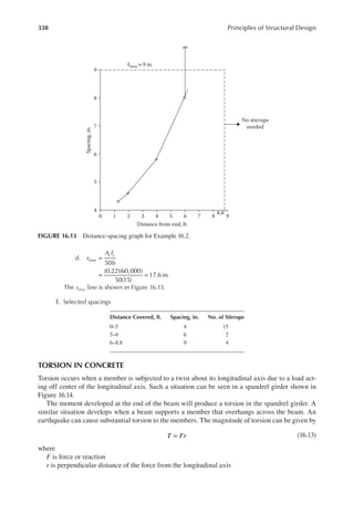
357. 339
Shear and Torsion in Reinforced Concrete
A load factor is applied to the torsion to convert T to Tu similar to the moment. A torsion produces
torsional shear on all faces of a member. The torsional shear leads to diagonal tensile stress very
similar to that caused by the lexure shear. The concrete will crack along the spiral lines that will
run at 45° from the faces of a member when this diagonal tension exceeds the strength of concrete.
After the cracks develop, any additional torsion will make the concrete fail suddenly unless tor-
sional reinforcement is provided. Similar to shear reinforcement, providing torsional reinforcement
will not change the magnitude of the torsion at which the cracks will form. However, once the
cracks are formed the torsional tension will be taken over by the torsional reinforcement to provide
additional strength against the torsional tension.
PROVISION FOR TORSIONAL REINFORCEMENT
ACI 318-11 provides that as long as the factored applied torsion, Tu, is less than one-fourth of the
cracking torque Tr, torsional reinforcement is not required. Equating Tu to one-fourth of cracking
torque Tr, the threshold limit is expressed as
[ ]
2
= φ ′
T f
A
P
a
u limit C
cp
cp
(16.14)
where
Tu is factored design torsion
Acp is area enclosed by the outside parameter of the concrete section = width × height
Spandrel
girder
Girder
Spandrel
girder
Girder
Slab
Beams
Beam
Action point of
load on beam
FIGURE 16.14 Beam subjected to torsion.

358. 340 Principles of Structural Design
Pcp is outside parameter of concrete = 2 (b + h)
ϕ = 0.75 for torsion
When Tu exceeds the above threshold limit, torsional reinforcement has to be designed. The process
consists of performing the following computations:
1. Verifying from Equation 16.14 that the cross-sectional dimensions of the member are suf-
iciently large to support the torsion acting on the beam.
2. If required, designing the closed loop stirrups to support the torsional tension (Tu = ϕTn) as
well as the shear-induced tension (Vu = ϕVn).
3. Computing the additional longitudinal reinforcement to resist the horizontal compo-
nent of the torsional tension. There must be a longitudinal bar in each corner of the
stirrups.
When an appreciable torsion is present that exceeds the threshold value, it might be more
expedient and economical to select a larger section than would normally be chosen, to satisfy
Equation 16.14, so that torsional reinforcement does not have to be provided. The book uses this
approach.
Example 16.3
The concentrated service loads, as shown in Figure 16.15, are located at the end of a balcony
cantilever section, 6 in. to one side of the centerline. Is the section adequate without any torsional
reinforcement? If not, redesign the section so that no torsional reinforcement has to be provided.
Use fC
′ = 4,000 psi and fy = 60,000 psi.
SOLUTION
The beam is subjected to moment, shear force, and torsion. It is being analyzed for torsion only.
A. Checking the existing section
1. Design load contributing to torsion
Pu 1.2(10) 1.6(15) 36 k
= + =
2. Design torsion
Tu 36
6
12
18 ft. k
=





 =
4-#10
#3 @ 12 in. OC
21 in.
3 in.
18 in.
DL= 10 k
LL = 15 k
10 ft.
FIGURE 16.15 Cantilever beam and section for Example 16.3.

359. 341
Shear and Torsion in Reinforced Concrete
3. Area enclosed by the outside parameter
A bh
cp 18 24 432 in.2
= = × =
4. Outside parameter
P b h
cp 2( ) 2(18 24) 84 in.
= + = + =
5. Torsional capacity of concrete
f
A
P
C
cp
cp
NG
(0.75) 4000
(432)
84
105,385.2 in. lb or 8.78 ft.-k 18 k
2
2
= φ ′
=
= − <
B. Redesign the section
1. Assume a width of 24 in.
2. Area enclosed by the outside parameter Acp = (24h)
3. Parameter enclosed Pcp = 2(24 + h)
4. f
A
P
h
h
h
h
h
h
C
cp
cp
Torsional capacity
(0.75) 4000
(24 )
2(24 )
13,661
(24 )
in. lb or 1.138
(24 )
ft.-k
2
2
2 2
= φ ′
=
+
=
+
−
+
5. For no torsional reinforcement
T f
A
P
u C
cp
cp
2
= φ ′
or
=
+
h
h
18 1.138
(24 )
2
or
=
h 29 in.
A section 24 × 29 will be adequate.
PROBLEMS
16.1–16.3 Determine the concrete shear capacity, web reinforcement shear capacity,
and design shear force permitted on the beam sections shown in Figures P16.1
through P16.3. Check for the spacing of web reinforcement. Use fc′ = 3,000 psi and
fy = 40,000 psi.
16.4 A reinforced beam of span 20 ft. shown in Figure P16.4 is subjected to a dead load of
1 k/ft. (excluding beam weight) and live load of 2 k/ft. Is the beam satisfactory to resist
the maximum shear force? Use fc′ = 3,000 psi and fy = 60,000 psi.
16.5 The service dead load (excluding the beam) is one-half of the service live load on the
beam of span 25 ft. shown in Figure P16.5. What is the magnitude of these loads from
shear consideration? Use fc′ = 4,000 psi and fy = 60,000 psi.

360. 342 Principles of Structural Design
16.6 A simply supported beam is 15 in. wide and has an effective depth of 24 in. It supports a
total factored load of 10 k/ft. (including the beam weight) on a clear span of 22 ft. Design
the web reinforcement. Use fc′ = 4,000 psi and fy = 60,000 psi.
16.7 Design the web reinforcement for the service loads shown in Figure P16.6. Use fc′ = 4,000
psi and fy = 60,000 psi.
12 in.
4-#8
#3 @ 10 in. OC
20 in.
FIGURE P16.1 Beam section for Problem 16.1.
18 in.
5-#7
#4 @ 12 in. OC
32 in.
FIGURE P16.2 Beam section for Problem 16.2.
15 in.
10 in.
4-#5
(no web
reinforcement)
FIGURE P16.3 Beam section for Problem 16.3.
12 in.
4-#7
#3 @ 12 in. OC
18 in.
FIGURE P16.4 Beam section for Problem 16.4.
15 in.
4-#8
#3 @ 8in. OC
27 in.
FIGURE P16.5 Beam section for Problem 16.5.

361. 343
Shear and Torsion in Reinforced Concrete
16.8 For the beam and service loads shown in Figure P16.7, design the web reinforcement
using #4 stirrups. Use fc′ = 5,000 psi and fy = 60,000 psi.
16.9 For the service loads on a beam (excluding beam weight) shown in Figure P16.8, design
the web reinforcement. Use fc′ = 4,000 psi and fy = 50,000 psi.
16.10 Design the web reinforcement for the service loads on the beam shown in Figure P16.9.
Use fc′ = 3,000 psi and fy = 40,000 psi.
16.11 A simply supported beam carries the service loads (excluding the beam weight) shown in
Figure P16.10. Design the web reinforcement. Use fc′ = 4,000 psi and fy = 60,000 psi.
16.12 A simply supported beam carries the service loads (excluding the beam weight) shown in
Figure P16.11. Design the web reinforcement. Use #4 size stirrups. Use fc′ = 4,000 psi and
fy = 60,000 psi.
15 in.
4-#9
24 in.
15 ft.
1 ft. 1 ft.
DL= 4 k/ft. (including weight)
LL= 6 k/ft.
FIGURE P16.6 Loads on beam and section for Problem 16.7.
20 in.
5-#11
32 in.
30 ft.
DL = 5 k/ft. (excluding weight)
LL = 10 k/ft.
FIGURE P16.7 Loads on beam and section for Problem 16.8.
12 in.
4-#9
24 in.
20 ft.
DL= 2 k/ft.
LL= 4 k/ft.
FIGURE P16.8 Loads on beam and section for Problem 16.9.

362. 344 Principles of Structural Design
16.13 A cantilever beam carries the service loads, including the beam weight, shown in
Figure P16.12. Design the web reinforcement. Use fc′ = 4,000 psi and fy = 60,000 psi.
[Hint: Vcritical is at the support.]
16.14 A beam carries the factored loads (including beam weight) shown in Figure P16.13.
Design the #3 size web reinforcement. Use fc′ = 3,000 psi and fy = 40,000 psi.
16.15 A beam supported on the walls carries the uniform distributed loads and the concen-
trated loads from the upper loor shown in Figure P16.14. The loads are service loads
15 in.
5-#8
25 in.
Use #4
size
20 ft. 5 ft.
DL = 1 k/ft.
LL = 1.8k/ft.
DL=10 k
LL= 10 k
DL = 10k
LL= 10 k
5 ft.
FIGURE P16.11 Loads on beam and section for Problem 16.12.
15 in.
4-#9
30 in.
6 ft.
DL= 1 k/ft.
(excluding weight)
LL = 50 k 50 k
6 ft. 6 ft.
FIGURE P16.10 Loads on beam and section for Problem 16.11.
20 in.
5-#11
30 in.
15 ft. 15 ft.
DL = 1 k/ft. (excluding weight)
LL = 1 k/ft.
LL=10 k
FIGURE P16.9 Loads on beam and section for Problem 16.10.

363. 345
Shear and Torsion in Reinforced Concrete
including the weight of the beam. Design the #3 size web reinforcement. Use fc′ = 4,000 psi
and fy = 50,000 psi.
16.16 Determine the torsional capacity of the beam section in Figure P16.15 without torsional
reinforcement. Use fc′ = 4,000 psi and fy = 60,000 psi.
16.17 Determine the torsional capacity of the cantilever beam section shown in Figure P16.16
without torsional reinforcement. Use fc′ = 3,000 psi and fy = 40,000 psi.
12 in.
6-#8
20 in.
12 ft.
DL= 2 k/ft.
LL= 4 k/ft.
FIGURE P16.12 Loads on cantilever beam and section for Problem 16.13.
14 in.
4-#11
# 3 size
28 in.
5 @ 6 ft.= 30 ft.
2.5 k/ft.
15 k 15 k 15 k 15 k
FIGURE P16.13 Loads on beam and section for Problem 16.14.
20 in.
5-#11
# 3 size 30 in.
20 ft.
6 ft. 20 in.
20in.
DL = 50 k
LL = 60 k DL = 2 k/ft.
LL = 3k/ft.
FIGURE P16.14 Loads and section of beam.

364. 346 Principles of Structural Design
16.18 A spandrel beam shown in Figure P16.17 is subjected to a factored torsion of 8 ft.-k.
Is this beam adequate if no torsional reinforcement is used? If not, redesign the section.
The width cannot exceed 16 in. Use fc′ = 4,000 psi and fy = 50,000 psi.
16.19 Determine the total depth of a 24 in. wide beam if no torsional reinforcement is used. The
service loads, as shown in Figure P16.18, act 5 in. to one side of the centerline. Use fc′ =
4,000 psi and fy = 60,000 psi.
16.20 A spandrel beam is exposed to a service dead load of 8 k and live load of 14 k acting 8 in.
off center of the beam. The beam section is 20 in. wide and 25 in. deep. Is the section
adequate without torsional reinforcement? If not, redesign the section using the same
width. Use fc′ = 5,000 psi and fy = 60,000 psi.
16in.
21 in.
3 in.
4-#9
FIGURE P16.15 Beam section under torsion for Problem 16.16.
15 in.
20 in.
3 in.
4-#8
FIGURE P16.16 Cantilever section under torsion for Problem 16.17.
14in.
18 in.
3 in.
4-#9
FIGURE P16.17 Beam section under torsion for Problem 16.18.
DL=15 k
LL= 20 k
8 ft.
FIGURE P16.18 Torsional loads on cantilever for Problem 16.19.

365. 347
17 Compression and Combined
Forces Reinforced
Concrete Members
TYPES OF COLUMNS
Concrete columns are divided into four categories.
PEDESTALS
The column height is less than three times the least lateral dimension. A pedestal is designed with
plain concrete (without reinforcement) for a maximum compression strength of 0.85 ϕ fc′Ag, where
ϕ is 0.65 and Ag is the cross-sectional area of the column.
COLUMNS WITH AXIAL LOADS
The compressive load acts coinciding with the longitudinal axis of the column or at a small eccen-
tricity so that there is no induced moment or there is a moment of little signiicance. This is a basic
case although not quite common in practice.
SHORT COLUMNS WITH COMBINED LOADS
The columns are subjected to an axial force and a bending moment. However, the buckling effect is
not present and the failure is initiated by crushing of the material.
LARGE OR SLENDER COLUMNS WITH COMBINED LOADS
In this case the buckling effect is present. Due to an axial load, P, the column axis buckles by an
amount ∆. Thus, the column is subjected to the secondary moment or the P-∆ moment.
As concrete and steel both can share compression loads, steel bars directly add to the strength of
a concrete column. The compression strain is equally distributed between concrete and steel that
are bonded together. It causes a lengthwise shortening and a lateral expansion of the column due to
Poisson’s effect. The column capacity can be enhanced by providing a lateral restraint. The column
is known as a tied or a spiral column depending on whether the lateral restraint is in the form of the
closely spaced ties or the helical spirals wrapped around the longitudinal bars, as shown in Figure
17.1a and b.
Tied columns are ordinarily square or rectangular and spiral columns are round but they could
be otherwise too. The spiral columns are more effective in terms of the column strength because of
their hoop stress capacity. But they are more expensive. As such tied columns are more common and
spiral columns are used only for heavy loads.
The composite columns are reinforced by steel shapes that are contained within the concrete
sections or by concrete being illed in within the steel section or tubing as shown in Figure 17.1c and d.
The latter are commonly called the lally columns.

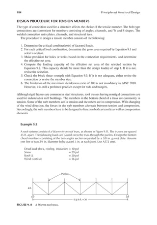
366. 348 Principles of Structural Design
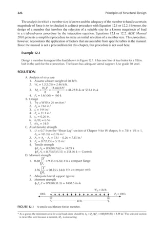
AXIALLY LOADED COLUMNS
This category includes columns with a small eccentricity. The small eccentricity is deined when
the compression load acts at a distance, e, from the longitudinal axis controlled by the following
conditions:
e h
Forspiralcolumns: 0.05
≤ (17.1)
e h
For tiedcolumns: 0.1
≤ (17.2)
where h is column dimension along distance, e.
In the case of columns, unlike beams, it does not matter whether the concrete or steel reaches
ultimate strength irst because both of them deform/strain together, which distributes the matching
stresses between them.
Also, high strength is more effective in columns because the entire concrete area contributes to
the strength, unlike the contribution from concrete in the compression zone only in beams, which
is about 30%–40% of the total area.
The basis of design is the same as for wood or steel columns, that is,
P P
u n
≤ φ (17.3)
where
Pu is factored axial load on the column
Pn is nominal axial strength
ϕ = strength reduction factor
= 0.70 for spiral column
= 0.65 for tied column
The nominal strength is the sum of the strength of concrete and the strength of steel. The concrete
strength is the ultimate (uniform) stress 0.85 fc′ times the concrete area (Ag − Ast) and the steel
strength is the yield stress, fy, times the steel area, Ast. However, to account for the small eccentricity,
a factor (0.85 for spiral and 0.8 for tied) is applied.
Thus,
0.85[0.85 ( ) ]forspiralcolumns
P f A A f A
n c g st y st
= ′ − + (17.4)
0.80[0.85 ( ) ]for tiedcolumns
P f A A f A
n c g st y st
= ′ − + (17.5)
Including a strength reduction factor of 0.7 for spiral and 0.65 for tied columns in the previous equa-
tions, Equation 17.3 for column design is as follows:
For spiral columns with e ≤ 0.05h
0.60[0.85 ( ) ]
P f A A f A
u c g st y st
= ′ − + (17.6)
(a) (b) (c) (d)
FIGURE 17.1 Types of columns: (a) tied column, (b) spiral column, and (c) and (d) composite columns.

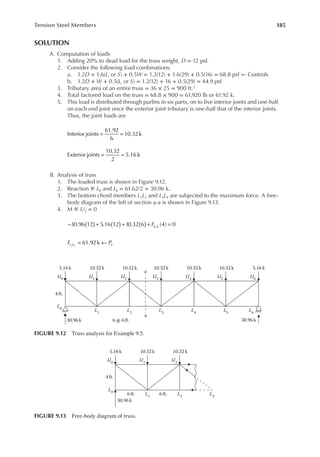
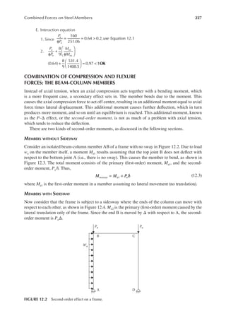
367. 349
Compression and Combined Forces Reinforced Concrete Members
For tied columns with e ≤ 0.1 h
0.52[0.85 ( ) ]
P f A A f A
u c g st y st
= ′ − + (17.7)
STRENGTH OF SPIRALS
It could be noticed that a higher factor is used for spiral columns than tied columns. The reason is
that in a tied column, as soon as the shell of a column spalls off, the longitudinal bars will buckle
immediately with the lateral support gone. But a spiral column will continue to stand and resist
more load with the spiral and longitudinal bars forming a cage to conine the concrete.
Because the utility of a column is lost once its shell spalls off, the American Concrete Institute
(ACI) assigns only slightly more strength to the spiral as compared to strength of the shell that gets
spalled off.
With reference to Figure 17.2,
Strengthof shell 0.85 ( )
f A A
c g c
= ′ − (a)
Hooptensioninspiral 2 2
f A f A
y sp y s c
= = ρ (b)
where ρs is spiral steel ratio = Asp/Ac.
Equating the two expressions (a) and (b) and solving for ρs,
ρ =
′
−






f
f
A
A
s
c
y
g
c
0.425 1 (c)
Ac
db
Core
area
Shell area
(Ag–Ac)
Ds
Dc
fy Asp
fʹ
y Asp
h
s =pitch
FIGURE 17.2 Spiral column section and proile.

368. 350 Principles of Structural Design
Making the spiral a little stronger,
ρ =
′
−






f
f
A
A
s
c
y
g
c
0.45 1 (17.8)
Once the spiral steel is determined, the following expression derived from the deinition of ρs is used
to set the spacing or pitch of the spiral.
By deinition, from Figure 17.2,
volumeof spiralinoneloop
volumeof concreteinpitch,s
s
ρ = (d)
( )
( /4)
2
D d A
D s
c b sp
c
=
π −
π
(e)
If the diameter difference, that is, db, is neglected,
4A
D s
s
sp
c
ρ = (f)
or
4
s
A
D
sp
c s
=
ρ
(17.9)
Appendix D, Table D.13, based on Equations 17.8 and 17.9, can be used to select the size and
pitch of spirals for a given diameter of a column.
SPECIFICATIONS FOR COLUMNS
1. Main steel ratio: The steel ratio, ρg, should not be less than 0.01 (1%) and not more than
0.08. Usually a ratio of 0.03 is adopted.
2. Minimum number of bars: A minimum of four bars are used within the rectangular or
circular ties and six within the spirals.
3. Cover: A minimum cover over the ties or spiral shall be 11
2 in.
4. Spacing: The clear distance between the longitudinal bars should neither be less than 1.5
times the bar diameter nor11
2 in. To meet these requirements, Appendix D, Table D.14 can
be used to determine the maximum number of bars that can be accommodated in one row
within a given size of a column.
5. Tie requirements:
a. The minimum size of the tie bars is #3 when the size of longitudinal bars is #10 or smaller
or when the column diameter is 18 in. or less. The minimum size is #4 for longitudinal
bars larger than #10 or a column larger than 18 in. Usually, #5 is the maximum size.
b. The center-to-center spacing of ties should be the smaller of the following:
i. 16 times the diameter of longitudinal bars
ii. 48 times the diameter of ties
iii. Least column dimension
c. The ties shall be so arranged that every corner and alternate longitudinal bar will have
the lateral support provided by the corner of a tie having an included angle of not more
than 135°. Figure 17.3 shows the tie arrangements for several columns.

369. 351
Compression and Combined Forces Reinforced Concrete Members
d. Longitudinal bar shall not have more than 6 in. clear distance on either side of a tie. If
it is more than 6 in., a tie is provided as shown in Figure 17.3c and e.
6. Spiral requirements:
a. The minimum spiral size is 3/8 in. (#3). Usually the maximum size is 5/8 in. (#5).
b. The clear space between spirals should not be less than 1 in. or more than 3 in.
ANALYSIS OF AXIALLY LOADED COLUMNS
The analysis of columns of small eccentricity involves determining the maximum design load
capacity and verifying the amount and details of the reinforcement according to the code. The pro-
cedure is summarized below:
1. Check that the column meets the eccentricity requirement (≤0.05h for spiral and ≤0.1h for
tied column).
2. Check that the steel ratio, ρg, is within 0.01–0.08.
3. Check that there are at least four bars for a tied column and six bars for a spiral column
and that the clear spacing between bars is determined according to the “Speciications for
Columns” section.
4. Calculate the design column capacity using Equation 17.6 or 17.7.
5. For ties, check the size, spacing, and arrangement using the information in the
“Speciications for Columns” section. For spirals, check the size and spacing using the
information in the “Speciications for Columns” section.
(b) (c)
(a)
(e) (f)
(d)
(h) (i)
(g)
≤6in.
≤ 6 in.
> 6 in.
>6 in.
6 in. max. 6 in. max.
FIGURE 17.3 Tie arrangements for several columns (a) through (i).

370. 352 Principles of Structural Design
Example 17.1
Determine the design axial load on a 16 in. square axially loaded column reinforced with eight
#8 size bars. Ties are #3 at 12 in. on center. Use fc′ = 4,000 psi and fy = 60,000 psi.
SOLUTION
1. Ast = 6.32 in.2 (from Appendix D, Table D.2)
2. Ag = 16 × 16 = 256 in.2
3.
6.32
256
0.0247
A
A
g
st
g
ρ = = =
This is >0.01 and <0.08 OK
4. h = 2(cover) + 2(tie diameter) + 3(bar diameter) + 2(spacing)
or 16 = 2(1.5) + 2(0.375) + 3(1) + 2(s)
or s = 4.625 in.
smin = 1.5(1) = 1.5 in., spacing s is more than smin OK
smax = 6 in., spacing s is less than smax OK
5. From Equation 17.7
0.52[0.85(4,000)(256 6.32) (60,000)(6.32)]
1,000
638.6 k
Pu =
− +
=
6. Check the ties
a. #3 size OK
b. The spacing should be the smaller of the following:
i. 16 × 1 = 16 in. ← Controls, more than given 12 in. OK
ii. 48 × 0.375 = 18 in.
iii. 16 in.
c. Clear distance from the tie = 4.625 in. (step 4) < 6 in. OK
Example 17.2
A service dead load of 150 k and live load of 220 k is axially applied on a 15 in. diameter circular
spiral column reinforced with six #9 bars. The lateral reinforcement consists of 3/8 in. spiral at 2 in.
on center. Is the column adequate? Use fc′ = 4,000 psi and fy = 60,000 psi.
SOLUTION
1. Ast = 6 in.2 (from Appendix D, Table D.2)
2.
4
(15) 176.63in.
2 2
Ag =
π
=
3.
6
176.63
0.034
A
A
g
st
g
ρ = = =
This is >0.01 and <0.08: OK
4. 2 cover 2 spiral diameter
15 2 1
.5 2 0.375 11
.25 in.
D d h
c b ( )
( ) ( )
( ) ( )
− = − −
= − − =
5. Perimeter, p = π(Dc − db) = π(11.25) = 35.33 in.
p = 6(bar diameter) + 6(spacing)
or 35.33 = 6(1.128) + 6(s)
or s = 4.76 in.
smin = 1.5(1) = 1.5 in., spacing s is more than smin OK
smax = 6 in., spacing s is less than smax OK
6. ϕ 0.60[0.85(4,000)(176.63 6) (60,000)(6)]
1,000
564 k
Pn =
− +
=

371. 353
Compression and Combined Forces Reinforced Concrete Members
7. 1
.2 150 1
.6 220 532 k 564 k
Pu ( ) ( )
= + = < OK
8. Check for spiral
a. 3/8 in. diameter OK
Dc = 15 − 3 = 12 in.
b.
4
(12) 113.04 in.
0.11 in.
2 2
2
A
A
c
sp
=
π
=
=
From Equation 17.8
0.45
(4)
(60)
176.63
113.04
1 0.017
s
ρ = −





 =
From Equation 17.9
OK
4(0.11)
(12)(0.017)
2.16 in. 2 in. (given)
s = = >
c. Clear distance = 2 − 3/8 = 1.625 in. > 1 in. OK
DESIGN OF AXIALLY LOADED COLUMNS
Design involves ixing of the column dimensions, selecting reinforcement, and deciding the size
and spacing of ties and spirals. For a direct application, Equations 17.6 and 17.7 are rearranged as
follows by substituting Ast = ρgAg.
For spiral columns:
0.60 [0.85 (1 ) ]
P A f f
u g c g y g
= ′ − ρ + ρ (17.10)
For tied columns:
0.52 [0.85 (1 ) ]
P A f f
u g c g y g
= ′ − ρ + ρ (17.11)
The design procedure involves the following:
1. Determine the factored design load for various load combinations.
2. Assume ρg = 0.03. A lower or higher value could be taken depending upon a bigger or
smaller size of column being acceptable.
3. Determine the gross area, Ag, from Equation 17.10 or 17.11. Select the column dimensions
to a full-inch increment.
4. For the actual gross area, calculate the adjusted steel area from Equation 17.6 or 17.7.
Make the selection of steel using Appendix D, Table D.2 and check from Appendix D,
Table D.14 that the number of bars can it in a single row of the column.
5. (For spirals) select the spiral size and pitch from Appendix D, Table D.13. (For ties) select
the size of tie, decide the spacing, and arrange ties as per item 5 of “Speciications for
Columns” section.
6. Sketch the design.
Example 17.3
Design a tied column for an axial service dead load of 200 k and service live load of 280 k. Use
fc′ = 4,000 psi and fy = 60,000 psi.

372. 354 Principles of Structural Design
SOLUTION
1. 1
.2 200 1
.6 280 688 k
Pu ( ) ( )
= + =
2. For ρg = 0.03, from Equation 17.11,
A
P
f f
g
u
c g y g
=
′ − ρ + ρ
=
− +
=
0.52[0.85 (1 ) ]
688
0.52[0.85(4)(1 0.03) 60(0.03)]
259.5 in.2
For a square column, 259.5 16.1
h = = in., use 16 in. × 16 in., Ag = 256 in.2
3. From Equation 17.7,
688 = 0.52 [0.85(4)(256 − Ast) + 60(Ast)]
688 = 0.52(870.4 + 56.6Ast)
Ast = 8 in.2
Select 8 bars of #9 size, Ast (provided) = 8 in.2
From Appendix D, Table D.14, for a core size of 16 − 3 = 13 in., 8 bars of #9 size can be
arranged in a row.
4. Design of ties:
a. Select #3 size
b. Spacing should be the smaller of the following:
i. 16(1.128) = 18 in.
ii. 48(0.375) = 18 in.
iii. 16 in. ← Controls
c. Clear distance
16 = 2(cover) + 2(tie diameter) + 3(bar diameter) + 2(spacing)
16 = 2(1.5) + 2 (0.375) + 3(1.128) + 2s
or s = 4.43 in. < 6 in. OK
5. The sketch is shown in Figure 17.4.
Example 17.4
For Example 17.3, design a circular spiral column.
SOLUTION
1. 1
.2 200 1
.6 280 688 k
Pu ( ) ( )
= + =
2. For ρg = 0.03, from Equation 17.10,
A
P
f f
g
u
c g y g
( )
[ ]
( ) ( )
=
′ ρ + ρ




=
− +
=
0.60 0.85 1–
688
0.60 0.85 1 0.03 60 0.03
225 in.2
16 in.
16in.
#3 at 16 in.
1½ in.
8-#9 bars
FIGURE 17.4 Tied column section of Example 17.3.

373. 355
Compression and Combined Forces Reinforced Concrete Members
For a circular column,
π
= =
4
225, 16.93 in.,
2
h
h use 17 in., Ag = 227 in.2
3. From Equation 17.6,
688 0.60 0.85 4 227 60
688 0.60 771
.8 56.6
or 6.62 in.2
A A
A
A
st st
st
st
( )
( ) ( )
( )
= − +

 

= +
=
Select 7 bars of #9 size, Ast (provided) = 7 in.2
From Appendix D, Table D.14, for a core size of 17 − 3 = 14 in., 9 bars of #9 can be
arranged in a single row. OK
4. Design of spiral:
a. From Appendix D, Table D.13, for 17 in. diameter column,
spiral size = 3/8 in.
pitch = 2 in.
b. Clear distance
2 − 0.375 = 1.625 in. > 1 in. OK
5. The sketch is shown in Figure 17.5.
SHORT COLUMNS WITH COMBINED LOADS
Most of the reinforced concrete columns belong to this category. The condition of an axial load-
ing or a small eccentricity is rare. The rigidity of the connection between beam and column makes
the column rotate with the beam resulting in a moment at the end. Even an interior column of
equally spanned beams will receive unequal loads due to variations in the applied loads, producing
a moment on the column.
Consider that a load, Pu, acts at an eccentricity, e, as shown in Figure 17.6a. Apply a pair of loads
Pu, one acting up and one acting down through the column axis, as shown in Figure 17.6b. The
applied loads cancel each other and, as such, have no technical signiicance. When we combine the
load Pu acting down at an eccentricity e with the load Pu acting upward through the axis, a couple,
Mu = Pue, is produced. In addition, the downward load Pu acts through the axis. Thus, a system
of force acting at an eccentricity is equivalent to a force and a moment acting through the axis, as
shown in Figure 17.6c. Inverse to this, a force and a moment when acting together are equivalent to
a force acting with an eccentricity.
As discussed with wood and steel structures, buckling is a common phenomenon associated with
columns. However, concrete columns are stocky and a great number of columns are not affected
by buckling. These are classiied as the short columns. It is the slenderness ratio that determines
17 in.
7 – #9 bars
1½ in.
3/8in. spiral at 2 in.
FIGURE 17.5 Spiral column of Example 17.4.

374. 356 Principles of Structural Design
whether a column could be considered a short or a slender (long) column. The ACI sets the follow-
ing limits when it is a short column and the slenderness effects could be ignored:
a. For members not braced against sidesway:
22
Kl
r
≤ (17.12)
b. For members braced against sidesway:
≤ −






34 12 1
2
Kl
r
M
M
(17.13a)
or
Kl
r
40
≤ (17.13b)
where
M1 and M2 are small and large end moments. The ratio M1/M2 is positive if a column bends in
a single curvature, that is, the end moments have opposite signs. It is negative for a double
curvature when the end moments have the same sign. (This is opposite of the sign conven-
tion for steel in the “Magniication Factor, B1” section in Chapter 12.)
l is length of column
K is effective length factor given in Figure 7.6 and the alignment charts in Figures 10.5 and 10.6
r = radius of gyration = I A
/
= 0.3h for rectangular column
= 0.25h for circular column
If a clear bracing system in not visible, the ACI provides certain rules to decide whether a frame is
braced or unbraced. However, conservatively it can be assumed to be unbraced.
The effective length factor has been discussed in detail in the “Column Stability Factor” section
in Chapter 7, and the “Effective Length Factor for Slenderness Ratio” section in Chapter 10. For
columns braced against sidesway, the effective length factor is 1 or less; conservatively it can be set
as 1. For members subjected to sidesway, the effective length factor is greater than 1. It is 1.2 for a
column ixed at one end and the other end has the rotation ixed but is free to translate (sway).
e e
Pu Pu
Pu
Pu Pu
Mu = Pu∙e
= =
(a) (b) (c)
FIGURE 17.6 Equivalent force system on a column: (a) eccentric load on a column, (b) equivalent loaded
column with axial and eccentric loads, and (c) equivalent column with axial load and moment.

375. 357
Compression and Combined Forces Reinforced Concrete Members
EFFECTS OF MOMENT ON SHORT COLUMNS
To consider the effect of an increasing moment (eccentricity) together with an axial force on a col-
umn, the following successive cases have been presented accompanied with respective stress/strain
diagrams.
ONLY AXIAL LOAD ACTING
The entire section will be subjected to a uniform compression stress, σc = Pu/Ag, and a uniform
strain of ε = σc/Ec, as shown in Figure 17.7. The column will fail by the crushing of concrete. By
another measure the column will fail when the compressive concrete strain reaches 0.003. In the
following other cases, the strain measure will be considered because the strain diagrams are linear.
The stress variations in concrete are nonlinear.
LARGE AXIAL LOAD AND SMALL MOMENT (SMALL ECCENTRICITY)
Due to axial load there is a uniform strain, −εc, and due to moment, there is a bending strain of
compression on one side and tension on the other side. The sum of these strains is shown in the last
diagram of Figure 17.8b. As the maximum strain due to the axial load and moment together cannot
exceed 0.003, the strain due to the load will be smaller than 0.003 because a part of the contribution
is made by the moment. Hence, the axial load Pu will be smaller than the previous case.
Pu
(a) (b) (c)
Max
0.003
–σc –εc
FIGURE 17.7 Axial load only on column: (a) load or column, (b) stress, (c) strain.
Pu
e
–εc + =
+εb
–εb
–εc+εb –εc–εb
Max .003
(a)
Strain due to
axial load
Strain due to
moment
(b) (c) (d)
FIGURE 17.8 Axial load with small moment on column: (a) load on column, (b) axial strain, (c) bending
strain, (d) combined strain.

376. 358 Principles of Structural Design
LARGE AXIAL LOAD AND MOMENT LARGER THAN CASE 2 SECTION
This is a case when the strain is zero at one face. To attain the maximum crushing strain of 0.003 on
the compression side, the strain contribution from both the axial load and moment will be 0.0015.
LARGE AXIAL LOAD AND MOMENT LARGER THAN CASE 3 SECTION
When the moment (eccentricity) increases somewhat from the previous case, the tension will
develop on one side of the column as the bending strain will exceed the axial strain. The entire ten-
sile strain contribution will come from steel.* The concrete on the compression side will contribute
to compression strain. The strain diagram will be as shown in Figure 17.10d. The neutral axis (the
point of zero strain) will be at a distance c from the compression face. As the strain in steel is less
than yielding, the failure will occur by crushing of concrete on the compression side.
BALANCED AXIAL LOAD AND MOMENT
As the moment (eccentricity) continues to increase, the tensile strain steadily rises. A condition will
be reached when the steel on the tension side will attain the yield strain, εy = fy/E (for Grade 60
steel, this strain is 0.002), simultaneously as the compression strain in concrete reaches the crushing
strain of 0.003. The failure of concrete will occur at the same time as steel yields. This is known as
the balanced condition. The strain diagrams in this case are shown in Figure 17.11. The value of c
in Figure 17.11d is less as compared to the previous case, that is, the neutral axis moves up toward
the compression side.
* The concrete being weak in tension, its contribution is neglected.
Pu
e
–εc –εc + =
+εb
εb
–εc +εb
–εc–εb
Max .003
(a) (b) (c) (d)
FIGURE 17.9 Axial load and moment (Case 3) on column: (a) load on column, (b) axial strain, (c) bending
strain, (d) combined strain.
Pu
e
–εc –εc –εb
+ =
+εb
εb–εc
–εc –εb
Max .003
(a) (b) (c) (d)
c
FIGURE 17.10 Axial load and moment (Case 4) on column: (a) load on column, (b) axial strain, (c) bending
strain, (d) combined strain.

377. 359
Compression and Combined Forces Reinforced Concrete Members
SMALL AXIAL LOAD AND LARGE MOMENT
As the moment (eccentricity) is further increased, steel will reach to the yield strain, εy = fy/E,
before concrete attains the crushing strain of 0.003. In other words, when compared to the concrete
strain of 0.003, the steel strain has already exceeded its yield limit, εy, as shown in Figure 17.12d.
The failure will occur by yielding of steel. This is called the tension-controlled condition.
NO APPRECIABLE AXIAL LOAD AND LARGE MOMENT
This is the case when the column acts as a beam. The eccentricity is assumed to be at ininity. The
steel has long before yielded prior to concrete reaching a level of 0.003. In other words, when com-
pared to a concrete strain of 0.003, the steel strain is 0.005 or more. This is shown in Figure 17.13b.
As discussed in the “Axially Loaded Columns” section, when a member acts as a column, the
strength (capacity) reduction factor, ϕ, is 0.7 for spiral columns and 0.65 for tied columns. This is
the situation for Cases 1 through 5. For beams, as in Case 7, the factor is 0.9. For Case 6, between
the column and the beam condition, the magnitude of ϕ is adjusted by Equation 14.13, based on the
value of strain in steel, εt.
If the magnitudes of the axial loads and the moments for all seven cases are plotted, it will appear
like the shape shown in Figure 17.14. This is known as the interaction diagram.
CHARACTERISTICS OF THE INTERACTION DIAGRAM
The interaction diagram presents the capacity of a column for various proportions of the loads and
moments. Any combination of loading that falls inside the diagram is satisfactory whereas any
combination falling outside represents a failure condition.
Pu
e
–εc –εc –εb
+ =
+εb
0.002
0.003
(a) (b) (c) (d)
c
FIGURE 17.11 Balanced axial load and moment (Case 5) on column: (a) load on column, (b) axial strain,
(c) bending strain, (d) combined strain.
Pu
e
ε
–εc εc
+
=
+εb –εb
When 0.003
(a) (b) (c) (d)
c
–εy>
fy
E
FIGURE 17.12 Small axial load and large moment (Case 6) on column: (a) load on column, (b) axial strain
(c) bending strain, (d) combined strain.

378. 360 Principles of Structural Design
From Cases 1 through 5 where compression control exists, as the axial load decreases the moment
capacity increases. Below this stage, the position is different. First of all, for the same moment, the
axial capacity is higher in the compression control zone than in the tensile control zone. Further
in the tensile control zone, as the axial load increases the moment capacity also increases. This is
due to the fact that any axial compression load tends to reduce the tensile strain (and stress), which
results in raising of the moment-resisting capacity.
Any radial line drawn from origin O to any point on the diagram represents a constant eccen-
tricity, that is, a constant ratio of the moment to the axial load. A line from point O to a point on
the diagram for the “Balanced Axial Load and Moment” (Case 5) condition represents the ebalanced
eccentricity.
Within the same column, as the amount of steel varies, although the shape of the diagram (curve)
remains similar to Figure 17.4, the location of the curve shifts to represent the appropriate magni-
tudes of the axial force and the moment; that is, the shapes of the curves are parallel.
The interaction diagram serves as a very useful tool in the analysis and design of columns for
the combined loads.
M
(a) (b)
When 0.003
εy≥ 0.005
c
FIGURE 17.13 Moment only column (Case 7): (a) load on column, (b) combined strain.
Figure 17.12
Figure 17.11
Figure 17.10
Figure 17.9
Figure 17.8
Figure 17.7
Tension
controlled
Compression
controlled
Balanced condition
e=ebalanced
Figure 17.13
Mu
Pu
O
FIGURE 17.14 Column interaction diagram.

379. 361
Compression and Combined Forces Reinforced Concrete Members
APPLICATION OF THE INTERACTION DIAGRAM
The ACI has prepared the interaction diagrams in dimensionless units for rectangular and circular
columns with different arrangements of bars for various grades of steel and various strengths of con-
crete. The abscissa has been represented as /
R M f A h
n u c g
= φ ′ and the ordinate as / .
K P f A
n u c g
= φ ′
Several of these diagrams for concrete strength of 4,000 psi and steel strength of 60,000 psi are
included in Appendix D, Tables D.15 through D.22.
On these diagrams, the radial strain line of value = 1 represents the balanced condition. Any point
on or above this line represents compression control and ϕ = 0.7 (spiral) or 0.65 (tied). Similarly
the line of εt = 0.005 represents that the steel has yielded or beam behavior. Any point on or below
this line will have ϕ = 0.9. In between these two lines is the transition zone for which ϕ has to be
corrected by Equation 14.13.
The line labeled Kmax indicates the maximum axial load with the limiting small eccentricity of
0.05h for spiral and 0.1h for tied columns.
The other terms in these diagrams are
1.
A
A
g
st
g
ρ =
2. h = column dimension in line with eccentricity (perpendicular to the plane of bending)
3.
center-to-center distance of outer row of steel
h
γ = (17.14)
4. Slope of radial line from origin = h/e
ANALYSIS OF SHORT COLUMNS FOR COMBINED LOADING
This involves determining the axial load strength and the moment capacity of a known column. The
steps comprise the following:
1. From Equation 17.12 or 17.13, conirm that it is a short column (there is no slenderness effect).
2. Calculate the steel ratio, ρg = Ast/Ag, and check for the value to be between 0.01 and 0.08.
3. Calculate γ from Equation 17.14
4. Select the right interaction diagram to be used based on γ, type of cross section, fc′, and fy.
5. Calculate the slope of the radial line = h/e
6. Locate a point for coordinates Kn = 1 and Rn = 1/slope, or Rn = e/h (or for any value of Kn,
Rn = Kne/h). Draw a radial line connecting the coordinate point to the origin. Extend the
line to intersect with ρg of step 2. If necessary, interpolate the interaction curve.
7. At the intersection point, read Kn and Rn.
8. If the intersection point is on or above the strain line = 1, ϕ = 0.7 or 0.65. If it is on or below
εt = 0.005, ϕ = 0.9. If it is in between, correct ϕ by Equation 14.13. This correction is rarely
applied.
9. Compute Pu = Knϕ fc′Ag and Mu = Rnϕ fc′Agh.
Example 17.5
A 10 ft. long braced column with a cross section is shown in Figure 17.15. Find the axial design
load and the moment capacity for an eccentricity of 6 in. The end moments are equal and have
the same sign. Use fc′ = 4,000 psi and fy = 60,000 psi.
SOLUTION
1. For same sign (double curvature), = −
M
M
1
1
2
.
2. K = 1 (braced), l = 10 × 12 = 120 in., r = 0.3h = 0.3(16) = 4.8 in.

380. 362 Principles of Structural Design
3. = =
Kl
r
1
(120)
4.8
25
4. Limiting value from Equation 17.13
Kl
r
M
M
= −






= − − = >
34 12
34 12( 1) 46 40
1
2
Limit value of 40 used
Since step (3) < step (4), short column
5. 16 16 256 in.
6.32 in.
2
2
A
A
g
st
= × =
=
6.32
256
0.025
g
ρ = =
6. Center to center of steel = 16 − 2(cover) − 2(tie diameter) − 1(bar diameter)
= 16 − 2(1.5) − 2(0.375) − 1(1) = 11.25 in.
γ = =
11.25
16
0.70
7. Use the interaction diagram in Appendix D, Table D.17
8. = = =
h
e
slope
16
6
2.67
9. 1,
1
slope
1
2.67
0.375
K R
n n
= = = =
Draw a radial line connecting the aforementioned coordinates to origin
10. At ρg = 0.025, Kn = 0.48 and Rn = 0.18
11. The point is above the line where strain = 1, hence ϕ = 0.65
12. Pu = Knϕfc′Ag = 0.48(0.65)(4)(256) = 319.5 k
Mu = Rnϕfc′Agh = 0.18(0.65)(4)(256)(16) = 1917 in.-k or 159.74 ft.-k.
DESIGN OF SHORT COLUMNS FOR COMBINED LOADING
This involves determining the size, selecting steel, and ixing ties or spirals for a column. The steps
are as follows:
1. Determine the design-factored axial load and moment.
2. Based on ρg = 1% and axial load only, estimate the column size by Equation 17.10 or 17.11,
rounding on the lower side.
3. For a selected size (diameter) of bars, estimate γ for the column size of step 2.
4. Select the right interaction diagram based on fc′, fy, the type of cross section, and γ of
step 3.
5. Calculate /
K P f A
n u c g
= φ ′ and /
R M f A h
n u c g
= φ ′ , assuming ϕ = 0.7 (spiral) or 0.65 (ties).
16 in.
16in.
#3 at 12 in.
1½ in.
8-# 8bars
FIGURE 17.15 Eccentrically loaded column for Example 17.5.

381. 363
Compression and Combined Forces Reinforced Concrete Members
6. Entering the appropriate diagram at Appendix D, Tables D.15 through D.22, read ρg at the
intersection point of Kn and Rn. This should be less than 0.05. If not, change the dimension
and repeat steps 3–6.
7. Check that the interaction point of step 6 is above the line where strain = 1. If not adjust ϕ
and repeat steps 5 and 6.
8. Calculate the required steel area, Ast = ρgAg and select reinforcement from Appendix D,
Table D.2 and check that it its in one row from Appendix D, Table D.14.
9. Design ties or spirals from steps 5 and 6 of the “Speciication for Columns” section.
10. Conirm from Equation 17.12 or 17.13 that the column is short (no slenderness effect).
Example 17.6
Design a 10 ft. long circular spiral column for a braced system to support service dead and live
loads of 300 k and 460 k, respectively, and service dead and live moments of 100 ft.-k each. The
moment at one end is zero. Use fc′ = 4,000 psi and fy = 60,000 psi.
SOLUTION
1. 1
.2 300 1
.6 460 1096 k
1
.2 100 1
.6 100 280 ft.-k or 3360 in.-k
P
M
u
u
( ) ( )
( ) ( )
= + =
= + =
2. Assume ρg = 0.01, from Equation 17.10:
0.60[0.85 (1 ) ]
1096
0.60[0.85(4)(1 0.01) 60(0.01)]
460.58 in.2
A
P
f f
g
u
c g y g
=
′ − ρ + ρ
=
− +
=
π
=
h
4
460.58
2
or h = 24.22 in.
Use h = 24 in., Ag = 452 in.2
3. Assume #9 size of bar and 3/8 in. spiral center-to-center distance
Center to center distance = 24 − 2(cover) − 2(spiral diameter) − 1(bar diameter)
= 24 − 2(1.5) − 2(3/8) − 1.128 = 19.12 in.
γ = =
19.12
24
0.8
Use the interaction diagram in Appendix D, Table D.21
4.
1096
(0.7)(4)(452)
0.866
3360
(0.7)(4)(452)(24)
0.11
K
P
f A
R
M
f A h
n
u
c g
n
u
c g
=
φ ′
= =
=
φ ′
= =
5. At the intersection point of Kn and Rn, ρg = 0.025
6. The point is above the strain line = 1, hence ϕ = 0.7 OK
7. 0.025 452 11
.3 in.2
Ast ( )( )
= =
From Appendix D, Table D.2, select 12 bars of #9, Ast = 12 in.2
From Appendix D, Table D.14 for a core diameter of 24 − 3 = 21 in., 15 bars of #9 can be
arranged in a row

382. 364 Principles of Structural Design
8. Selection of spirals
From Appendix D, Table D.13, size = 3/8 in., pitch = 21
4 in.
Clear distance = 2.25 − 3/8 = 1.875 > 1 in. OK
9. K = 1, l = 10 × 12 = 120 in., r = 0.25(24) = 6 in.
= =





 =
−





 =
Kl
r
M
M
M
M
1
(120)
6
20
0
34 12 34
1
2
1
2
Because (Kl/r) ≤ 34, short column.
LONG OR SLENDER COLUMNS
When the slenderness ratio of a column exceeds the limits given by Equation 17.12 or 17.13, it is
classiied as a long or slender column. In a physical sense, when a column bends laterally by an
amount, Δ, the axial load, P, introduces an additional moment equal to P Δ. When this P Δ moment
cannot be ignored, the column is a long or slender column.
There are two approaches to deal with this additional or secondary moment. The nonlinear
second-order analysis is based on a theoretical analysis of the structure under application of an
axial load, a moment, and the delection. As an alternative approach, the ACI provides a irst-
order method that magniies the moment acting on the column to account for the P–Δ effect. The
magniication expressions for the braced (nonsway) and unbraced (sway) frames are similar to the
steel magniication factors discussed in the “Magniication Factor, B1” section” in Chapter 12 and
the “Magniication Factor for Sway, B2” section in Chapter 12. After the moments are magniied,
the procedure for short columns from the “Analysis of Short Columns for Combined Loading” and
“Design of Short Columns for Combined Loading” sections can be applied for analysis and design
of the column using the interaction diagrams.
The computation of the magniication factors is appreciably complicated for concrete because of
the involvement of the modulus of elasticity of concrete and the moment of inertia with creep and
cracks in concrete.
A large percent of columns do not belong to the slender category. It is advisable to avoid the
slender columns whenever possible by increasing the column dimensions, if necessary. As a rule
of thumb, a column dimension of one-tenth of the column length in braced frames will meet the
short column requirement. For a 10 ft. length, a column of 1 ft. or 12 in. or more will be a short
braced column. For unbraced frames, a column dimension one-ifth of the length will satisfy the
short column requirement. A 10 ft. long unbraced column of 2 ft. or 24 in. dimension will avoid the
slenderness effect.
PROBLEMS
17.1 Determine the design axial load capacity and check whether the reinforcements meet
the speciications for the column shown in Figure P17.1. Use fc′ = 4,000 psi and fy =
60,000 psi.
17.2 Determine the design axial load capacity and check whether the reinforcements meet
the speciications for the column shown in Figure P17.2. Use fc′ = 4,000 psi and fy =
60,000 psi.

383. 365
Compression and Combined Forces Reinforced Concrete Members
17.3 Determine the design axial load capacity of the column in Figure P17.3 and check whether
the reinforcement is adequate. Use fc′ = 5,000 psi and fy = 60,000 psi.
17.4 Determine whether the maximum service dead load and live load carried by the col-
umn shown in Figure P17.4 are equal. Check for spiral steel. Use fc′ = 3,000 psi and
fy = 40,000 psi.
17.5 Compute the maximum service live load that may be axially placed on the column
shown in Figure P17.5. The service dead load is 150 k. Check for ties speciications. Use
fc′ = 3,000 psi and fy = 40,000 psi.
17.6 A service dead load of 100 k and service live load of 450 k are axially applied on a 20 in.
diameter circular column reinforced with six #8 bars. The cover is 11 2 in. and the spi-
ral size is 1 2 in. at a 2 in. pitch. Is the column adequate? Use fc′ = 4,000 psi and fy =
60,000 psi.
17.7 Design a tied column to carry a factored axial design load of 900 k. Use fc′ = 5,000 psi
and fy = 60,000 psi.
17.8 For Problem 17.7, design a circular spiral column.
12in.
12in.
#3 at 12 in. OC
4-# 9 bars
1½ in.
FIGURE P17.1 Column section for Problem 17.1.
20 in.
20 in.
#3 at 15 in. OC
8-# 9 bars
1½ in.
FIGURE P17.2 Column section for Problem 17.2.
15 in.
#7 bars
3/8 in. spiral at 2 in.
1½ in.
FIGURE P17.3 Column section for Problem 17.3.

384. 366 Principles of Structural Design
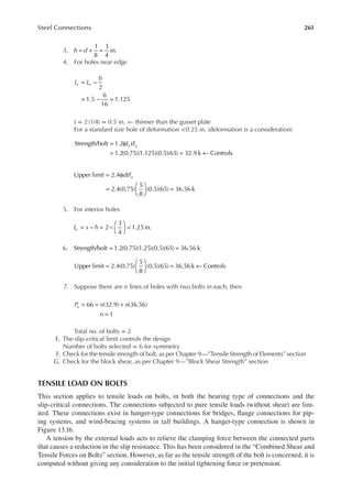
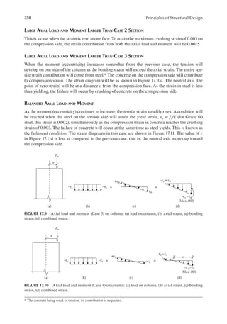
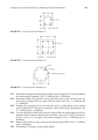
17.9 Design a tied column to support a service dead axial load of 300 k and live load of 480 k.
Use fc′ = 4,000 psi and fy = 60,000 psi.
17.10 Redesign a circular spiral column for Problem 17.9.
17.11 Design a rectangular tied column to support an axial service dead load of 400 k and live
load of 590 k. The larger dimension of the column is approximately twice the shorter
dimension. Use fc′ = 5,000 psi and fy = 60,000 psi.
17.12 Design the smallest circular spiral column to carry an axial service dead load of 200 k
and live load of 300 k. Use fc′ = 3,000 psi and fy = 60,000 psi. [Hint: For the smallest
dimension, use 8% steel and it is desirable to use #11 steel to reduce the number of bars
to be accommodated in a single row.]
17.13 For the 8 ft. long braced column shown in Figure P17.6, determine the axial load strength
and the moment capacity at an eccentricity of 5 in in the larger dimension. Use fc′ =
4,000 psi and fy = 60,000 psi.
17.14 An unbraced column shown in Figure P17.7 has a length of 8 ft. and a cross section as
shown. The factored moment-to-load ratio on the column is 0.5 ft. Determine the strength
of the column. K = 1.2. Use fc′ = 4,000 psi and fy = 60,000 psi.
17.15 On a 10 ft. long column of an unbraced frame system, the load acts at an eccentricity of
5 in. The column section is shown in Figure P17.8. What are the axial load capacity and
moment strength of the column? Use fc′ = 4,000 psi and fy = 60,000 psi.
#3 at 15 in. OC
18 in.
20 in.
8-# 10 bars
1½
FIGURE P17.5 Column section for Problem 17.5.
20 in.
15 in.
#3 at 12 in. OC
6 of #10
1½ in.
FIGURE P17.6 Column section for Problem 17.13.
18 in.
#9 bars
3/8in. spiral at 1½ in.
1½ in.
FIGURE P17.4 Column section for Problem 17.4.

385. 367
Compression and Combined Forces Reinforced Concrete Members
17.16 Design a 8 ft. long circular spiral column of a braced system to support a factored axial
load of 1200 k and a factored moment of 300 ft.-k. The end moments are equal and have
the same signs. Use fc′ = 4,000 psi and fy = 60,000 psi.
17.17 Design a tied column for Problem 17.16. Arrange the reinforcement on all faces.
17.18 For an unbraced frame, design a circular column of 10 ft. length that supports service
dead and live loads of 400 k and 600 k, respectively, and service dead and live moments
of 120 ft.-k and 150 ft.-k, respectively. The end moments are equal and have opposite
signs. K = 1.2. Use fc′ = 4,000 psi and fy = 60,000 psi.
17.19 Design a tied column for Problem 17.18 having reinforcement on all faces.
17.20 A braced frame has a 10 ft. long column. Design a tied column with reinforcing bars on
two end faces only to support the following service loads and moments. If necessary,
adjust the column dimensions to qualify it as a short column. The column has equal end
moments and a single curvature. Use fc′ = 4,000 psi and fy = 60,000 psi.
PD = 150 k, PL = 200 k
MD = 50 ft.-k, ML = 70 ft.-k.
22 in.
#9 bars
3/8 in. spiral at 2 in.
1½ in.
FIGURE P17.7 Column section for Problem 17.14.
#3 at 15 in. OC
8-#10 bars
22 in.
22 in.
1½ in.
FIGURE P17.8 Column section for Problem 17.15.

387. 369
Bibliography
Alsamsam, I. M. and Kamara, M. E. (eds.), Simpliied Design: Reinforced Concrete Buildings of Moderate Size
and Height, 3rd Ed., Portland Cement Association, Skokie, IL, 2004.
Ambrose, J. and Tripeny, P., Simpliied Engineering for Architects and Builders, John Wiley & Sons, Hoboken,
NJ, 2006.
Ambrose, J. and Tripeny, P., Building Structures, 3rd Ed., John Wiley & Sons, Hoboken, NJ, 2011.
American Concrete Institute, ACI Design Handbook, SP-17, American Concrete Institute, Farmington Hills,
MI, 1997.
American Concrete Institute, Building Code Requirements for Structural Concrete and Commentary, ACI
318-11, American Concrete Institute, Farmington Hills, MI, 2011.
American Forest & Paper Association, ASD/LRFD Manual for Engineered Wood Construction, 2012 Ed.,
AF&PA American Wood Council, Washington, DC, 2012.
American Forest & Paper Association, National Design Speciication for Wood Construction, 2012 Ed.,
AF&PA American Wood Council, Washington, DC, 2012.
American Forest & Paper Association, National Design Speciication Supplement, Design Values for Wood
Construction, AF&PA American Wood Council, Washington, DC, 2012.
American Forest & Paper Association, Solved Example Problems, ASD/LRFD, 2005 Ed., AF&PA American
Wood Council, Washington, DC, 2006.
American Forest & Paper Association, Special Design Provisions for Wind and Seismic, ASD/LRFD, 2008 Ed.,
AF&PA American Wood Council, Washington, DC, 2009.
American Institute of Steel Construction, Steel Construction Manual, 14th Ed. (2010 AISC Speciications),
American Institute of Steel Construction, Chicago, IL, 2011.
American Institute of Steel Construction, Seismic Design Manual, 2nd Ed. (2010 AISC Speciications),
American Institute of Steel Construction, Chicago, IL, 2013.
American Institute of Timber Construction, Timber Construction Manual, 6th Ed., John Wiley & Sons,
Hoboken, NJ, 2012.
American Society of Civil Engineers, Minimum Design Loads for Buildings and Other Structures, ASCE 7-10,
American Society of Civil Engineers, Reston, VA, 2010.
Breyer, D. E. et al., Design of Wood Structures, ASD/LRFD, 6th Ed., McGraw-Hill, New York, NY, 2007.
Brockenbrough, R. L. and Merritt, F. S., Structural Steel Designer’s Handbook, 5th Ed., ASCE Press, Reston,
VA, 2011.
Buckner, C. D., Concrete Design for the Civil and Structural PE Exams, Professional Publications, Belmont,
CA, 2012.
Building Seismic Safety Council, NEHRP Recommended Provisions: Design Examples, FEMA 451, National
Institute of Building Sciences, Washington, DC, 2006.
Building Seismic Safety Council, NEHRP Recommended Seismic Provisions for New Buildings and Other
Structures, 2009 Ed., FEMA P-750, National Institute of Building Sciences, Washington, DC, 2009.
Ching, F. D. and Winkel, S. R., Building Codes Illustrated: A Guide to Understanding the 2012 International
Building Code, 4th Ed., John Wiley & Sons, Hoboken, NJ, 2012.
Concrete Reinforcing Steel Institute, Manual of Standard Practice, 28th Ed., Concrete Reinforcing Steel
Institute, Chicago, IL, 2009.
Fanella, D. A., Seismic Detailing of Concrete Buildings, 2nd Ed., Portland Cement Association, Skokie, IL,
2007.
Federal Emergency Management Agency, Seismic Load Analysis, Federal Emergency Management Agency,
Washington, DC, 2006.
Fisher, J. M. et al., Technical Digest No 11—Design of Lateral Load Resisting Frames Using Steel Joists and
Joist Girders, Steel Joist Institute, Myrtle Beach, SC, 2007.
Galambos, T. V. et al., Basic Steel Design with LRFD, Prentice Hall, Englewood Cliffs, NJ, 1996.
Geschwinder, L. F., Design Steel Your Way with the 2005 AISC Speciications, American Institute of Steel
Construction, Chicago, IL, 2006.
Ghosh, S. K. and Shen, Q., Seismic and Wind Design of Concrete Buildings, Portland Cement Association,
Chicago, IL, 2009.

388. 370 Bibliography
Ghosh, S. K. et al., Signiicant Changes to the Seismic Load Provisions of ASCE 7-10: An Illustrated Guide,
ASCE Press, Reston, VA, 2011.
International Code Council, International Building Code, 2012, International Code Council, Country Club
Hills, IL, 2011.
International Code Council, International Residential Code for One- and Two-Family Dwellings, 2012,
International Code Council, Country Club Hills, IL, 2011.
Kamara, M. and Novak, L., Simpliied Design of Reinforced Concrete Buildings, Portland Cement Association,
Chicago, IL, 2011.
Kamara, M. E. (ed.), Notes on ACI 318-05 with Design Applications, Portland Cement Association, Skokie,
IL, 2005.
Limbrunner, G. F. and Aghayere, A. O., Reinforced Concrete Design, 7th Ed., Prentice Hall, Englewood Cliffs,
NJ, 2010.
McCormac, J. C. and Brown, R. H., Design of Reinforced Concrete, 8th Ed., John Wiley & Sons, Hoboken,
NJ, 2008.
McCormac, J. C. and Csernak, S. F., Structural Steel Design, 5th Ed., Prentice Hall, Upper Saddle River, NJ,
2011.
Mitchell, D. et al., AASHTO LRFD Strut-and-Tie Model: Design Examples, Engineering Bulletin, EB 231,
Portland Cement Association, Skokie, IL, 2004.
O’Rourke, M., Snow Loads: Guide to the Snow Load Provisions of ASCE 7-10, American Society of Civil
Engineers, Reston, VA, 2010.
Reese, R. C., CRSI Design Handbook, Literary Licensing, LLC, MT, 2012.
Roland, F. S., Steel Design for the Civil PE and Structural SE Exams, Professional Publications, Belmont,
CA, 2012.
Segui, W. T., Steel Design, 5th Ed., Cengage Learning, Stamford, CT, 2012.
Simiu, E. Design of Buildings for Wind: A Guide for ASCE 7-10 Standard Users and Designers of Special
Structures, John Wiley & Sons, Hoboken, NJ, 2011.
Stafford, T. E., Signiicant Changes to the Wind Load Provisions of ASCE 7-10: An Illustrated Guide, ASCE
Press, Reston, VA, 2010.
Steel Joist Institute, Standard Speciication for Joist Girders, American National Standard SJI-JG-1.1, Revised
November 2003, Steel Joist Institute, Forest, VA, 2005.
Steel Joist Institute, Standard Speciication for Open Web Steel Joists, K-series, American National Standard
SJI-K-1.1, Revised November 2003, Steel Joist Institute, Forest, VA, 2005.
Steel Joist Institute, Standard Speciications and Load and Weight Tables for Steel Joists and Joist Girders,
43rd Ed., Steel Joist Institute, Forest, VA, 2010.
Steel Joist Institute, SJI Publications Package, Steel Joist Institute, Forest, VA, 2012.
Underwood, R. and Chiuini, M., Structural Design: A Practical Guide for Architects, 2nd Ed., John Wiley &
Sons, Hoboken, NJ, 2007.
Whitney, C. S., Plastic theory of reinforced concrete design. Transactions of the American Society of Civil
Engineers, 68, 1942, pp. 251–326.
Wilden, H., FPCI (ed.), PCI Design Handbook: Precast and Prestressed Concrete, 7th Ed., Precast/Prestressed
Concrete Institute, Chicago, IL, 2010.
Williams, A., Steel Structures Design, ASD/LRFD, McGraw-Hill, New York, NY, 2011.
Winkel, S. R. et al., Building Codes Illustrated for Elementary and Secondary Schools, John Wiley & Sons,
Hoboken, NJ, 2007.
Wright, J. K. and MacGregor, J. G., Reinforced Concrete: Mechanics and Design, 6th Ed., Prentice Hall, Upper
Saddle River, NJ, 2011.

389. 371
Appendix A: General
TABLE A.1
Useful Conversion Factors
Multiply By To Obtain
Pounds (m) 0.4356 Kilogram
Kilogram 2.205 Pounds (m)
Mass in slug 32.2 Weight in pound
Mass in kilogram 9.81 Weight in Newton (N)
Pound (f) 4.448 Newton
Newton 0.225 Pounds
U.S. or short ton 2000 Pounds
Metric ton 1000 Kilogram
U.S. ton 0.907 Metric ton
Foot 0.3048 Meter
Meter 3.281 Feet
Mile 5280 Feet
Mile 1609 Meter
1.609 Kilometer
Square feet 0.0929 Square meter
Square mile 2.59 Square kilometer
Square kilometer 100 Hectare (ha)
Liter 1000 Cubic centimeter
Pounds per ft.2 47.88 N/m2 or pascal
Standard atmosphere 101.325 Kilopascal (kPa)
Horsepower 550 Foot-pound/second
745.7 Newton-meter/second or Watt
°F 5/9(°F − 32) °C
°C 9/5(°C + 32) °F
Log to base e (i.e., loge,
where e = 2.718)
0.434 Log to base 10 (i.e., log10)
TABLE A.2
Geometric Properties of Common Shapes
X
X
Y
b
Y
h
Rectangle:
A = bh,
Ix =
rx = = 0.288h.
1
bh3
,
12
Ix
A
(Continued)

390. 372 Appendix A
TABLE A.2 (continued)
Geometric Properties of Common Shapes
Triangle:
A = bh,
y =
Ix=
h ,
,
3
1
2
b+ m
bh3.
3
36
1
x =
x
b
y
h
n
m
X
X
Y
Y
X
R
X
Y
Y
D
Circle:
A = πD2
=πR2
,
Ix = = ,
,
1
4
64
πD4
4
πR4
J = Ix+ Iy= = .
32
πD4
2
πR4
rx= =
Ix
A
D
4
= R
2
y
X
Y
Y Semicircle:
A = πD2 = πR2 ,
= ,
,
1
8
1
2
3π
4r
Iy =
Ix = 0.00682D4
= 0.11R4
,
rx= 0.264R.
=
πD4
128
πR4
8
y
x
Y
Vertex
y
a
b
X
Parabola:
A = ab,
2
3
= b,
3
8
x
= a.
2
5
y
Vertex
b
a
Spandrel of parabola:
A =
x=
y =
y
x
1
3
ab,
3
4
b,
3
10
a.

391. 373
Appendix
A
TABLE A.3
Shears, Moments, and Delections
Loading Shear Force Diagram Moment Diagram
Maximum
Moment Slope at End
Maximum
Delection
l
P
x
l
R
R
2
l
2
l
P
x
R2
R1
a b
l
P
P
x
R
R
a a
l
wl
x
l
R
R
2
l
2
V1
V2
Shear
V
V
Shear
V
x
V
Shear
l
V
V
Shear
Moment
Mmax
Moment
Mmax
Moment
Mmax
Moment
Mmax
Pl
4
Pl
EI
16
2
Pl
EI
48
3
Pab
l
at x = a
Pa l a
EI
( )
−
6
2 2
at R2
Pb l b
EIl
( )
−
9 3
2 2 3/2
x
l b
=
−
at
3
2 2
Pa Pa l a
EI
( )
−
2
Pa l a
EI
( )
−
3 4
24
2 2
wl
8
2
wl
EI
24
3
wl
EI
5
384
4
(Continued)

392. 374
Appendix
A
TABLE A.3 (continued)
Shears, Moments, and Delections
Loading Shear Diagram Moment Diagram
Maximum
Moment Slope at End
Maximum
Delection
l
w
x
R1 R2
w
x
R R
l
2
l
2
l
P
R
x
l
x
R
P
l
a b
Shear
0.5774 l
V2
V1
Shear V
V
Shear
V
Shear
V
Moment
Mmax
Moment
0.5774 l
Mmax
Moment Mmax
Moment
Mmax
wl
9 3
2
wl
EI
8
360
3
at R2
wl
EI
2.5
384
4
at x =
0.519l
wl
12
2
wl
EI
5
192
3
wl
EI
120
4
−Pl Pl
EI
2
2
Pl
EI
3
3
−Pb Pl
EI
2
2
Pb l b
EI
( )
−
3
6
2
at free end

393. 375
Appendix
A
l
x
R
wl
P
l
x
R
R
l
2
l
2
wl
l
x
R
R
l
2
l
2
l
x
R
w
Shear V
Shear
V
Shear
V
V
Shear
V
V
Moment Mmax
Mmax
Moment
M1
Mmax
0.211 l
Moment
Mmax
Mmax
4
Moment
l
wl
−
2
2
wl
EI
6
3
wl
EI
8
4
wl
−
6
2
wl
EI
24
3
wl
EI
8
4
Pl
−
8
0 Pl
EI
192
3
wl
−
12
2 0 wl
EI
384
4
Note: w, load per unit length; W, total load.

394. 376 Appendix A
TABLE A.4
Typical Properties of Engineering Materials
Strength (psi) (Yield Values
Except Where Noted)
Modulus of
Elasticity (e)
(ksi)
Coeficient of
Thermal Expansion
(F–1) (10–6)
Material Tension Compression Shear
Wood (dry)
Douglas ir 6,000 3,500a 500 1,500 2
Redwood 6,500 4,500a 450 1,300 2
Southern Pine 8,500 5,000a 600 1,500 3
Steel 50,000 50,000 30,000 29,000 6.5
Concrete
Structural, lightweight 150b 3,500b 130b 2,100 5.5
Brick masonry 300b 4,500b 300b 4,500 3.4
Aluminum, structural 30,000 30,000 18,000 10,000 12.8
Iron, cast 20,000b 85,000b 25,000b 25,000 6
Glass, plate 10,000b 36,000b — 10,000 4.5
Polyester, glass-reinforced 10,000b 25,000b 25,000b 1,000 35
a For the parallel-to-grain direction.
b Denotes ultimate strength for brittle materials.

395. 377
Appendix B: Wood

396. 378
Appendix
B
TABLE B.1
Section Properties of Standard Dressed (S4S) Sawn Lumber
x–x Axis y–y Axis
Approximate Weight in Pounds per Linear Foot (lb/ft.) of Piece When
Density of Wood Equals
Nominal
Size
(b × d)
Standard
Dressed Size
(S4S) (b × d)
(in. × in.)
Area of
Section
A (in.2)
Section
Modulus
Sxx (in.3)
Moment
of Inertia
ixx (in.4)
Section
Modulus
Syy (in.3)
Moment
of Inertia
iyy (in.4) 25 lbs/ft3 30 lbs/ft3 35 lbs/ft3 40 lbs/ft3 45 lbs/ft3 50 lbs/ft3
Boards
1 × 3 3/4 × 2 1/2 1.875 0.781 0.977 0.234 0.088 0.326 0.391 0.456 0.521 0.586 0.651
1 × 4 3/4 × 3 1/2 2.625 1.531 2.680 0.328 0.123 0.456 0.547 0.638 0.729 0.820 0.911
1 × 6 3/4 × 5 1/2 4.125 3.781 10.40 0.516 0.193 0.716 0.859 1.003 1.146 1.289 1.432
1 × 8 3/4 × 7 1/4 5.438 6.570 23.82 0.680 0.255 0.944 1.133 1.322 1.510 1.699 1.888
1 × 10 3/4 × 9 1/4 6.938 10.70 49.47 0.867 0.325 1.204 1.445 1.686 1.927 2.168 2.409
1 × 12 3/4 × 11 1/4 8.438 15.82 88.99 1.055 0.396 1.465 1.758 2.051 2.344 2.637 2.930
Dimension Lumber (see NDS 4.1.3.2) and Decking (see NDS 4.1.3.5)
2 × 3 1 1/2 × 2 1/2 3.750 1.56 1.953 0.938 0.703 0.651 0.781 0.911 1.042 1.172 1.302
2 × 4 1 1/2 × 3 1/2 5.250 3.06 5.359 1.313 0.984 0.911 1.094 1.276 1.458 1.641 1.823
2 × 5 1 1/2 × 4 1/2 6.750 5.06 11.39 1.688 1.266 1.172 1.406 1.641 1.875 2.109 2.344
2 × 6 1 1/2 × 5 1/2 8.250 7.56 20.80 2.063 1.547 1.432 1.719 2.005 2.292 2.578 2.865
2 × 8 1 1/2 × 7 1/4 10.88 13.14 47.63 2.719 2.039 1.888 2.266 2.643 3.021 3.398 3.776
2 × 10 1 1/2 × 9 1/4 13.88 21.39 98.93 3.469 2.602 2.409 2.891 3.372 3.854 4.336 4.818
2 × 12 1 1/2 × 11 1/4 16.88 31.64 178.0 4.219 3.164 2.930 3.516 4.102 4.688 5.273 5.859
2 × 14 1 1/2 × 13 1/4 19.88 43.89 290.8 4.969 3.727 3.451 4.141 4.831 5.521 6.211 6.901
3 × 4 2 1/2 × 3 1/2 8.75 5.10 8.932 3.646 4.557 1.519 1.823 2.127 2.431 2.734 3.038
3 × 5 2 1/2 × 4 1/2 11.25 8.44 18.98 4.688 5.859 1.953 2.344 2.734 3.125 3.516 3.906
3 × 6 2 1/2 × 5 1/2 13.75 12.60 34.66 5.729 7.161 2.387 2.865 3.342 3.819 4.297 4.774
3 × 8 2 1/2 × 7 1/4 18.13 21.90 79.39 7.552 9.440 3.147 3.776 4.405 5.035 5.664 6.293
3 × 10 2 1/2 × 9 1/4 23.13 35.65 164.9 9.635 12.04 4.015 4.818 5.621 6.424 7.227 8.030
3 × 12 2 1/2 × 11 1/4 28.13 52.73 296.6 11.72 14.65 4.883 5.859 6.836 7.813 8.789 9.766
3 × 14 2 1/2 × 13 1/4 33.13 73.15 484.6 13.80 17.25 5.751 6.901 8.051 9.201 10.35 11.50

397. 379
Appendix
B
3 × 16 2 1/2 × 15 1/4 38.13 96.90 738.9 15.89 19.86 6.619 7.943 9.266 10.59 11.91 13.24
4 × 4 3 1/2 × 3 1/2 12.25 7.15 12.51 7.146 12.51 2.127 2.552 2.977 3.403 3.828 4.253
4 × 5 3 1/2 × 4 1/2 15.75 11.81 26.58 9.188 16.08 2.734 3.281 3.828 4.375 4.922 5.469
4 × 6 3 1/2 × 5 1/2 19.25 17.65 48.53 11.23 19.65 3.342 4.010 4.679 5.347 6.016 6.684
4 × 8 3 1/2 × 7 1/4 25.38 30.66 111.1 14.80 25.90 4.405 5.286 6.168 7.049 7.930 8.811
4 × 10 3 1/2 × 9 1/4 32.38 49.91 230.8 18.89 33.05 5.621 6.745 7.869 8.993 10.12 11.24
4 × 12 3 1/2 × 11 1/4 39.38 73.83 415.3 22.97 40.20 6.836 8.203 9.570 10.94 12.30 13.67
4 × 14 3 1/2 × 13 1/4 46.38 102.41 678.5 27.05 47.34 8.051 9.661 11.27 12.88 14.49 16.10
4 × 16 3 1/2 × 15 1/4 53.38 135.66 1,034 31.14 54.49 9.266 11.12 12.97 14.83 16.68 18.53
Timbers (5 in. × 5 in. and larger)
Post and Timber (see NDS 4.1.3.4)
5 × 5 4 1/2 × 4 1/2 20.25 15.19 34.17 15.19 34.17 3.516 4.219 4.922 5.625 6.328 7.031
6 × 6 5 1/2 × 5 1/2 30.25 27.73 76.26 27.73 76.26 5.252 6.302 7.352 8.403 9.453 10.50
6 × 8 5 1/2 × 7 1/4 39.88 48.18 174.7 36.55 100.5 6.923 8.307 9.69 11.08 12.46 13.85
8 × 8 7 1/4 × 7 1/4 52.56 63.51 230.2 63.51 230.2 9.125 10.95 12.78 14.60 16.43 18.25
8 × 10 7 1/4 × 9 1/4 67.06 103.4 478.2 81.03 293.7 11.64 13.97 16.30 18.63 20.96 23.29
10 × 10 9 1/4 × 9 1/4 85.56 131.9 610.1 131.9 610.1 14.85 17.83 20.80 23.77 26.74 29.71
10 × 12 9 1/4 × 11 1/4 104.1 195.1 1,098 160.4 742.0 18.07 21.68 25.29 28.91 32.52 36.13
12 × 12 11 1/4 × 11 1/4 126.6 237.3 1,335 237.3 1,335 21.97 26.37 30.76 35.16 39.55 43.95
12 × 14 11 1/4 × 13 1/4 149.1 329.2 2,181 279.5 1,572 25.68 31.05 36.23 41.41 46.58 51.76
14 × 14 13 1/4 × 13 1/4 175.6 387.7 2,569 387.7 2,569 30.48 36.58 42.67 48.77 54.86 60.96
14 × 16 13 1/4 × 15 198.8 496.9 3,727 438.9 2,908 34.51 41.41 48.31 55.21 62.11 69.01
16 × 16 15 × 15 225.0 562.5 4,219 562.5 4,219 39.06 46.88 54.69 62.50 70.31 78.13
16 × 18 15 × 17 255.0 722.5 6,141 637.5 4,781 44.27 53.13 61.98 70.83 79.69 88.54
18 × 18 17 × 17 289.0 818.8 6,960 818.8 6,960 50.17 60.21 70.24 80.28 90.31 100.3
18 × 20 17 × 19 323.0 1,023 9,717 915.2 7,779 56.08 67.29 78.51 89.72 100.9 112.2
20 × 20 19 × 19 361.0 1,143 10,860 1,143 10,860 62.67 75.21 87.7 100.3 112.8 125.3
20 × 22 19 × 21 399.0 1,397 14,663 1,264 12,003 69.27 83.13 97.0 110.8 124.7 138.5
22 × 22 21 × 21 441.0 1,544 16,207 1,544 16,207 76.56 91.88 107.2 122.5 137.8 153.1
22 × 24 21 × 23 483.0 1,852 21,292 1,691 17,750 83.85 100.6 117.4 134.2 150.9 167.7
24 × 24 23 × 23 529.0 2,028 23,320 2,028 23,320 91.84 110.2 128.6 146.9 165.3 183.7
(Continued)

398. 380
Appendix
B
TABLE B.1 (continued)
Section Properties of Standard Dressed (S4S) Sawn Lumber
x–x Axis y–y Axis
Approximate Weight in Pounds per Linear Foot (lb/ft.) of Piece When
Density of Wood Equals
Nominal
Size
(b × d)
Standard
Dressed Size
(S4S) (b × d)
(in. × in.)
Area of
Section
A (in.2)
Section
Modulus
Sxx (in.3)
Moment
of Inertia
ixx (in.4)
Section
Modulus
Syy (in.3)
Moment
of Inertia
iyy (in.4) 25 lbs/ft3 30 lbs/ft3 35 lbs/ft3 40 lbs/ft3 45 lbs/ft3 50 lbs/ft3
Beams and Stringers (see NDS 4.1.3.3)
6 × 10 5 1/2 × 9 1/4 50.88 78 363 47 128 8.83 10.6 12.4 14.1 15.9 17.7
6 × 12 5 1/2 × 11 1/4 61.88 116.0 653 56.72 156.0 10.74 12.89 15.04 17.19 19.34 21.48
6 × 14 5 1/2 × 13 1/4 72.88 160.9 1,066 66.80 183.7 12.65 15.18 17.71 20.24 22.77 25.30
6 × 16 5 1/2 × 15 82.50 206.3 1,547 75.63 208.0 14.32 17.19 20.05 22.92 25.78 28.65
6 × 18 5 1/2 × 17 93.50 264.9 2,252 85.71 235.7 16.23 19.48 22.73 25.97 29.22 32.47
6 × 20 5 1/2 × 19 104.5 330.9 3,144 95.79 263.4 18.14 21.77 25.40 29.03 32.66 36.28
6 × 22 5 1/2 × 21 115.5 404.3 4,245 105.9 291.2 20.05 24.06 28.07 32.08 36.09 40.10
6 × 24 5 1/2 × 23 126.5 484.9 5,577 116.0 318.9 21.96 26.35 30.75 35.14 39.53 43.92
8 × 12 7 1/2 × 11 1/4 81.6 152.9 860.2 98.6 357.3 14.16 16.99 19.82 22.66 25.49 28.32
8 × 14 7 1/4 × 13 1/4 96.1 212.1 1,405 116.1 420.8 16.68 20.01 23.35 26.68 30.02 33.36
8 × 16 7 1/4 × 15 108.8 271.9 2,039 131.4 476.3 18.88 22.66 26.43 30.21 33.98 37.76
8 × 18 7 1/4 × 17 123.3 349.2 2,968 148.9 539.9 21.40 25.68 29.96 34.24 38.52 42.80
8 × 20 7 1/4 × 19 137.8 436.2 4,144 166.4 603.4 23.91 28.70 33.48 38.26 43.05 47.83
8 × 22 7 1/4 × 21 152.3 532.9 5,595 184.0 666.9 26.43 31.72 37.01 42.29 47.58 52.86
8 × 24 7 1/4 × 23 166.8 639.2 7,351 201.5 730.4 28.95 34.74 40.53 46.32 52.11 57.90
10 × 14 9 1/4 × 13 1/4 122.6 270.7 1,793 189.0 873.9 21.28 25.53 29.79 34.05 38.30 42.56
10 × 16 9 1/4 × 15 138.8 346.9 2,602 213.9 989 24.09 28.91 33.72 38.54 43.36 48.18
10 × 18 9 1/4 × 17 157.3 445.5 3,787 242.4 1,121 27.30 32.76 38.22 43.68 49.14 54.60
10 × 20 9 1/4 × 19 175.8 556.5 5,287 270.9 1,253 30.51 36.61 42.72 48.82 54.92 61.02
10 × 22 9 1/4 × 21 194.3 679.9 7,139 299.5 1,385 33.72 40.47 47.21 53.96 60.70 67.45
10 × 24 9 1/4 × 23 212.8 815.5 9,379 328.0 1,517 36.94 44.32 51.71 59.10 66.48 73.87
12 × 16 11 1/4 × 15 168.8 421.9 3,164 316.4 1,780 29.30 35.16 41.02 46.88 52.73 58.59
12 × 18 11 1/4 × 17 191.3 541.9 4,606 358.6 2,017 33.20 39.84 46.48 53.13 59.77 66.41

399. 381
Appendix
B
12 × 20 11 1/4 × 19 213.8 676.9 6,430 400.8 2,254 37.11 44.53 51.95 59.38 66.80 74.22
12 × 22 11 1/4 × 21 236.3 826.9 8,682 443.0 2,492 41.02 49.22 57.42 65.63 73.83 82.03
12 × 24 11 1/4 × 23 258.8 992 11,407 485.2 2,729 44.92 53.91 62.89 71.88 80.86 89.84
14 × 18 13 1/4 × 17 225.3 638.2 5,425 497.4 3,295 39.11 46.93 54.75 62.57 70.39 78.21
14 × 20 13 1/4 × 19 251.8 797.2 7,573 555.9 3,683 43.71 52.45 61.19 69.93 78.67 87.41
14 × 22 13 1/4 × 21 278.3 974 10,226 614.5 4,071 48.31 57.97 67.63 77.29 86.95 96.6
14 × 24 13 1/4 × 23 304.8 1,168 13,434 673.0 4,459 52.91 63.49 74.07 84.65 95.23 105.8
16 × 20 15 × 19 285.0 902.5 8,574 712.5 5,344 49.48 59.38 69.27 79.17 89.06 99.0
16 × 22 15 × 21 315.0 1,103 11,576 787.5 5,906 54.69 65.63 76.56 87.50 98.4 109.4
16 × 24 15 × 23 345.0 1,323 15,209 862.5 6,469 59.90 71.88 83.85 95.8 107.8 119.8
18 × 22 17 × 21 357.0 1,250 13,120 1,012 8,598 61.98 74.38 86.77 99.2 111.6 124.0
18 × 24 17 × 23 391.0 1,499 17,237 1,108 9,417 67.88 81.46 95.03 108.6 122.2 135.8
20 × 24 19 × 23 437.0 1,675 19,264 1,384 13,146 75.87 91.04 106.2 121.4 136.6 151.7
Source: Courtesy of the American Wood Council.
Note: NDS, National Design Speciication.

400. 382 Appendix B
TABLE B.2
Size Factor and Flat Use Factor (All Species except Southern Pine)
Flat Use Factor, cfu
Bending design values adjusted by size factors are based on edgewise use (load applied to narrow face). When dimension
lumber is used latwise (load applied to wide face), the bending design value, Fb, shall also be multiplied by the following
lat use factors:
Thickness (Breadth)
Width (Depth) 2 in. and 3 in. 4 in.
2 in. and 3 in. 1.0 —
4 in. 1.1 1.0
5 in. 1.1 1.05
6 in. 1.15 1.05
8 in. 1.15 1.05
10 in. and wider 1.2 1.1
Size Factor, cF
Tabulated bending, tension, and compression parallel to grain design values for dimension lumber 2 in.–4 in. thick shall be
multiplied by the following size factors:
Fb
Thickness (Breadth)
Grades Width (Depth) 2 in. and 3 in. 4 in. Ft Fc
Select structural,
No. 1 and Btr,
No. 1, No. 2, No. 3
2 in., 3 in., and 4 in. 1.5 1.5 1.5 1.15
5 in. 1.4 1.4 1.4 1.1
6 in. 1.3 1.3 1.3 1.1
8 in. 1.2 1.3 1.2 1.05
10 in. 1.1 1.2 1.1 1.0
12 in. 1.0 1.1 1.0 1.0
14 in. and wider 0.9 1.0 0.9 0.9
Stud 2 in., 3 in., and 4 in. 1.1 1.1 1.1 1.05
5 in. and 6 in. 1.0 1.0 1.0 1.0
8 in. and wider Use No. 3 Grade tabulated design values and
size factors
Construction,
standard
2 in., 3 in., and 4 in. 1.0 1.0 1.0 1.0
Utility 4 in. 1.0 1.0 1.0 1.0
2 in. and 3 in. 0.4 — 0.4 0.6

401. 383
Appendix
B
TABLE B.2
Reference Design Values for Visually Graded Dimension Lumber (2–4 in. Breadth) (All Species except Southern Pine)
Design Values in Pounds per Square Inch (psi)
Species and
Commercial
Grade
Size
Classiication Bending, Fb
Tension
Parallel to
Grain, Ft
Shear
Parallel to
Grain, Fv
Compression
Perpendicular
to Grain, Fc⊥
Compression
Parallel to
Grain, Fc
Modulus of Elasticity
Grading Rules
Agency
e emin
Beech-Birch-Hickory
Select structural 2 in. and wider 1,450 850 195 715 1,200 1,700,000 620,000 NELMA
No. 1 1,050 600 195 715 950 1,600,000 580,000
No. 2 1,000 600 195 715 750 1,500,000 550,000
No. 3 575 350 195 715 425 1,300,000 470,000
Stud 2 in. and wider 775 450 195 715 475 1,300,000 470,000
Construction 2–4 in. wide 1,150 675 195 715 1,000 1,400,000 510,000
Standard 650 375 195 715 775 1,300,000 470,000
Utility 300 175 195 715 500 1,200,000 440,000
Cottonwood
Select structural 2 in. and wider 875 525 125 320 775 1,200,000 440,000 NSLB
No. 1 625 375 125 320 625 1,200,000 440,000
No. 2 625 350 125 320 475 1,100,000 400,000
No. 3 350 200 125 320 275 1,000,000 370,000
Stud 2 in. and wider 475 275 125 320 300 1,000,000 370,000
Construction 2–4 in. wide 700 400 125 320 650 1,000,000 370,000
Standard 400 225 125 320 500 900,000 330,000
Utility 175 100 125 320 325 900,000 330,000
Douglas Fir-Larch
Select structural 2 in. and wider 1,500 1,000 180 625 1,700 1,900,000 690,000 WCLIB
No. 1 and Btr 1,200 800 180 625 1,550 1,800,000 660,000 WWPA
(Continued)

402. 384
Appendix
B
TABLE B.2 (Continued)
Reference Design Values for Visually Graded Dimension Lumber (2–4 in. Breadth) (All Species except Southern Pine)
Design Values in Pounds per Square Inch (psi)
Species and
Commercial
Grade
Size
Classiication Bending, Fb
Tension
Parallel to
Grain, Ft
Shear
Parallel to
Grain, Fv
Compression
Perpendicular
to Grain, Fc⊥
Compression
Parallel to
Grain, Fc
Modulus of Elasticity
Grading Rules
Agency
e emin
No. 1 1,000 675 180 625 1,500 1,700,000 620,000
No. 2 900 575 180 625 1,350 1,600,000 580,000
No. 3 525 325 180 625 775 1,400,000 510,000
Stud 2 in. and wider 700 450 180 625 850 1,400,000 510,000
Construction 2–4 in. wide 1,000 650 180 625 1,650 1,500,000 550,000
Standard 575 375 180 625 1,400 1,400,000 510,000
Utility 275 175 180 625 900 1,300,000 470,000
Douglas Fir-Larch (North)
Select structural 2 in. and wider 1,350 825 180 625 1,900 1,900,000 690,000 NLGA
No. 1 and Btr 1,150 750 180 625 1,800 1,800,000 660,000
No. 1/No. 2 850 500 180 625 1,400 1,600,000 580,000
No. 3 475 300 180 625 825 1,400,000 510,000
Stud 2 in. and wider 650 400 180 625 900 1,400,000 510,000
Construction 2–4 in. wide 950 575 180 625 1,800 1,500,000 550,000
Standard 525 325 180 625 1,450 1,400,000 510,000
Utility 250 150 180 625 950 1,300,000 470,000
Douglas Fir (South)
Select structural 2 in. and wider 1,350 900 180 520 1,600 1,400,000 510,000 WWPA
No. 1 925 600 180 520 1,450 1,300,000 470,000
No. 2 850 525 180 520 1,350 1,200,000 440,000
No. 3 500 300 180 520 775 1,100,000 400,000
Stud 2 in. and wider 675 425 180 520 850 1,100,000 400,000
Construction 2–4 in. wide 975 600 180 520 1,650 1,200,000 440,000

403. 385
Appendix
B
Standard 550 350 180 520 1,400 1,100,000 400,000
Utility 250 150 180 520 900 1,000,000 370,000
Eastern Hemlock-Balsam Fir
Select structural 2 in. and wider 1,250 575 140 335 1,200 1,200,000 440,000 NELMA
No. 1 775 350 140 335 1,000 1,100,000 400,000 NSLB
No. 2 575 275 140 335 825 1,100,000 400,000
No. 3 350 150 140 335 475 900,000 330,000
Stud 2 in. and wider 450 200 140 335 525 900,000 330,000
Construction 2–4 in. wide 675 300 140 335 1,050 1,000,000 370,000
Standard 375 175 140 335 850 900,000 330,000
Utility 175 75 140 335 550 800,000 290,000
Eastern Hemlock-Tamarack
Select structural 2 in. and wider 1,250 575 170 555 1,200 1,200,000 440,000 NELMA
No. 1 775 350 170 555 1,000 1,100,000 400,000 NSLB
No. 2 575 275 170 555 825 1,100,000 400,000
No. 3 350 150 170 555 475 900,000 330,000
Stud 2 in. and wider 450 200 170 555 525 900,000 330,000
Construction 2–4 in. wide 675 300 170 555 1,050 1,000,000 370,000
Standard 375 175 170 555 850 900,000 330,000
Utility 175 75 170 555 550 800,000 290,000
Eastern Softwoods
Select structural 2 in. and wider 1,250 575 140 335 1,200 1,200,000 440,000 NELMA
No. 1 775 350 140 335 1,000 1,100,000 400,000 NSLB
No. 2 575 275 140 335 825 1,100,000 400,000
No. 3 350 150 140 335 475 900,000 330,000
Stud 2 in. and wider 450 200 140 335 525 900,000 330,000
Construction 2–4 in. wide 675 300 140 335 1,050 1,000,000 370,000
Standard 375 175 140 335 850 900,000 330,000
Utility 175 75 140 335 550 800,000 290,000
(Continued)

404. 386
Appendix
B
TABLE B.2 (Continued)
Reference Design Values for Visually Graded Dimension Lumber (2–4 in. Breadth) (All Species except Southern Pine)
Design Values in Pounds per Square Inch (psi)
Species and
Commercial
Grade
Size
Classiication Bending, Fb
Tension
Parallel to
Grain, Ft
Shear
Parallel to
Grain, Fv
Compression
Perpendicular
to Grain, Fc⊥
Compression
Parallel to
Grain, Fc
Modulus of Elasticity
Grading Rules
Agency
e emin
Eastern White Pine
Select structural 2 in. and wider 1,250 575 135 350 1,200 1,200,000 440,000 NELMA
No. 1 775 350 135 350 1,000 1,100,000 400,000 NSLB
No. 2 575 275 135 350 825 1,100,000 400,000
No. 3 350 150 135 350 475 900,000 330,000
Stud 2 in. and wider 450 200 135 350 525 900,000 330,000
Construction 2–4 in. wide 675 300 135 350 1,050 1,000,000 370,000
Standard 375 175 135 350 850 900,000 330,000
Utility 175 75 135 350 550 800,000 290,000
Hem-Fir
Select structural 2 in. and wider 1,400 925 150 405 1,500 1,600,000 580,000 WCLIB
No. 1 and Btr 1,100 725 150 405 1,350 1,500,000 550,000 WWPA
No. 1 975 625 150 405 1,350 1,500,000 550,000
No. 2 850 525 150 405 1,300 1,300,000 470,000
No. 3 500 300 150 405 725 1,200,000 440,000
Stud 2 in. and wider 675 400 150 405 800 1,200,000 440,000
Construction 2–4 in. wide 975 600 150 405 1,550 1,300,000 470,000
Standard 550 325 150 405 1,300 1,200,000 440,000
Utility 250 150 150 405 850 1,100,000 400,000
Hem-Fir (North)
Select structural 2 in. and wider 1,300 775 145 405 1,700 1,700,000 620,000 NLGA
No. 1 and Btr 1,200 725 145 405 1,550 1,700,000 620,000
No. 1/No. 2 1,000 575 145 405 1,450 1,600,000 580,000
No. 3 575 325 145 405 850 1,400,000 510,000

405. 387
Appendix
B
Stud 2 in. and wider 775 450 145 405 925 1,400,000 510,000
Construction 2–4 in. wide 1,150 650 145 405 1,750 1,500,000 550,000
Standard 650 350 145 405 1,500 1,400,000 510,000
Utility 300 175 145 405 975 1,300,000 470,000
Mixed Maple
Select structural 2 in. and wider 1,000 600 195 620 875 1,300,000 470,000 NELMA
No. 1 725 425 195 620 700 1,200,000 440,000
No. 2 700 425 195 620 550 1,100,000 400,000
No. 3 400 250 195 620 325 1,000,000 370,000
Stud 2 in. and wider 550 325 195 620 350 1,000,000 370,000
Construction 2–4 in. wide 800 475 195 620 725 1,100,000 400,000
Standard 450 275 195 620 575 1,000,000 370,000
Utility 225 125 195 620 375 900,000 330,000
Source: Courtesy of the American Forest & Paper Association, Washington, DC.
Notes: Tabulated design values are for normal load duration and dry service conditions. See NDS 4.3 for a comprehensive description of design value adjustment factors.

406. 388 Appendix B
TABLE B.3
Size Factor and Flat Use Factor for Southern Pine
Flat Use Factor, cfu
Bending design values adjusted by size factors are based on edgewise use (load applied to narrow face). When dimension
lumber is used latwise (load applied to wide face), the bending design value, Fb, shall also be multiplied by the following
lat use factors:
Thickness (breadth)
Width (depth) 2 in. and 3 in. 4 in.
2 in. and 3 in. 1.0 —
4 in. 1.1 1.0
5 in. 1.1 1.05
6 in. 1.15 1.05
8 in. 1.15 1.05
10 in. and wider 1.2 1.1
Size Factor, cF
Appropriate size adjustment factors have already been included in the tabular design values of Southern Pine and mixed
Southern Pine dimension lumber, except the following cases:
Grade Size Fb Fc Ft Fv, Fc⊥, e, emin
All grades (except Dense
Structural 86, Dense
Structural 72, Dense
Structural 65)
(1) For 4-in. breadth × 8 in.
or more depth
1.1
(2) For all dimension lumber
>12-in. depth, the table values of
12-in. depth multiplied as shown
across
0.9 0.9 0.9 1.00
Dense Structural 86, Dense
Structural 72, Dense
Structural 65
For dimension lumber >12-in.
depth, Fb table value of 12 in.
multiplied as shown across
(12/ )1/9
d

407. 389
Appendix
B
TABLE B.3
Reference Design Values for Visually Graded Southern Pine Dimension Lumber (2 in.–4 in. Thick)
Design Values in Pounds per Square Inch (psi)
Species and Commercial
Grade
Size
Classiication Bending Fb
Tension
Parallel to
Grain Ft
Shear
Parallel to
Grain Fv
Compression
Perpendicular to
Grain Fc⊥
Compression
Parallel to
Grain Fc
Modulus of Elasticity
Speciic
Gravity G
Grading
Rules Agency
e emin
Southern Pine
Dense select structural 2 in.–4 in. wide 3,050 1,650 175 660 2,250 1,900,000 690,000 0.55 SPIB
Select structural 2,850 1,600 175 565 2,100 1,800,000 660,000
Nondense select structural 2,650 1,350 175 480 1,950 1,700,000 620,000
No. 1 Dense 2,000 1,100 175 660 2,000 1,800,000 660,000
No. 1 1,850 1,050 175 565 1,850 1,700,000 620,000
No. 1 Nondense 1,700 900 175 480 1,700 1,600,000 580,000
No. 2 Dense 1,150 750 175 660 1,250 1,500,000 550,000
No. 2 1,050 650 175 565 1,100 1,400,000 510,000
No. 2 Nondense 975 575 175 480 1,050 1,200,000 440,000
No. 3 and stud 600 375 175 565 625 1,200,000 440,000
Construction 4 in. wide 800 500 175 565 1,150 1,300,000 470,000 0.55
Standard 450 275 175 565 950 1,200,000 440,000
Utility 200 125 175 565 625 1,100,000 400,000
Dense select structural 5 in.–6 in. wide 2,700 1,500 175 660 2,150 1,900,000 690,000 0.55
Select structural 2,550 1,400 175 565 2,000 1,800,000 660,000
Nondense select structural 2,350 1,200 175 480 1,850 1,700,000 620,000
No. 1 Dense 1,750 950 175 660 1,900 1,800,000 660,000
No. 1 1,650 900 175 565 1,750 1,700,000 620,000
No. 1 Nondense 1,500 800 175 480 1,600 1,600,000 580,000
No. 2 Dense 1,450 775 175 660 1,750 1,700,000 620,000
No. 2 1,250 725 175 565 1,600 1,600,000 580,000
No. 2 Nondense 1,150 675 175 480 1,500 1,400,000 510,000
(Continued)

408. 390
Appendix
B
TABLE B.3 (continued)
Reference Design Values for Visually Graded Southern Pine Dimension Lumber (2 in.–4 in. Thick)
Design Values in Pounds per Square Inch (psi)
Species and Commercial
Grade
Size
Classiication
Bending
Fb
Tension
Parallel to
Grain Ft
Shear
Parallel to
Grain Fv
Compression
Perpendicular
to Grain Fc⊥
Compression
Parallel to
Grain Fc
Modulus of Elasticity
Speciic
Gravity G
Grading
Rules Agency
e emin
Southern Pine
No. 3 and stud 750 425 175 565 925 1,400,000 510,000
Dense select structural 8 in. wide 2,450 1,350 175 660 2,050 1,900,000 690,000 0.55
Select structural 2,300 1,300 175 565 1,900 1,800,000 660,000
Non-dense select structural 2,100 1,100 175 480 1,750 1,700,000 620,000
No. 1 Dense 1,650 875 175 660 1,800 1,800,000 660,000
No. 1 1,500 825 175 565 1,650 1,700,000 620,000
No. 1 Non-dense 1,350 725 175 480 1,550 1,600,000 580,000
No. 2 Dense 1,400 675 175 660 1,700 1,700,000 620,000
No. 2 1,200 650 175 565 1,550 1,600,000 580,000
No. 2 Nondense 1,100 600 175 480 1,450 1,400,000 510,000
No. 3 and stud 700 400 175 565 875 1,400,000 510,000
Dense select structural 10 in. wide 2,150 1,200 175 660 2,000 1,900,000 690,000 0.55
Select structural 2,050 1,100 175 565 1,850 1,800,000 660,000
Nondense select structural 1,850 950 175 480 1,750 1,700,000 620,000
No. 1 Dense 1,450 775 175 660 1,750 1,800,000 660,000
No. 1 1,300 725 175 565 1,600 1,700,000 620,000
No. 1 Nondense 1,200 650 175 480 1,500 1,600,000 580,000
No. 2 Dense 1,200 625 175 660 1,650 1,700,000 620,000
No. 2 1,050 575 175 565 1,500 1,600,000 580,000
No. 2 Nondense 950 550 175 480 1,400 1,400,000 510,000
No. 3 and stud 600 325 175 565 850 1,400,000 510,000

409. 391
Appendix
B
Dense select structural 12 in. wide 2,050 1,100 175 660 1,950 1,900,000 690,000 0.55
Select structural 1,900 1,050 175 565 1,800 1,800,000 660,000
Nondense select structural 1,750 900 175 480 1,700 1,700,000 620,000
No. 1 Dense 1,350 725 175 660 1,700 1,800,000 660,000
No. 1 1,250 675 175 565 1,600 1,700,000 620,000
No. 1 Nondense 1,150 600 175 480 1,500 1,600,000 580,000
No. 2 Dense 1,150 575 175 660 1,600 1,700,000 620,000
No. 2 975 550 175 565 1,450 1,600,000 580,000
No. 2 Nondense 900 525 175 480 1,350 1,400,000 510,000
No. 3 and stud 575 325 175 565 825 1,400,000 510,000
Southern Pine (Surfaced Dry – Used in dry service conditions – 19% or less moisture content)
Dense structural 86 2 in. and wider 2,600 1,750 175 660 2,000 1,800,000 660,000 0.55 SPIB
Dense structural 72 2,200 1,450 175 660 1,650 1,800,000 660,000
Dense structural 65 2,000 1,300 175 660 1,500 1,800,000 660,000
Southern Pine (Surfaced Green – Used in any service condition)
Dense structural 86 2,100 1,400 165 440 1,300 1,600,000 580,000 0.55 SPIB
Dense structural 72 2–1/2 in. and
wider
1,750 1,200 165 440 1,100 1,600,000 580,000
Dense structural 65 2–1/2 in.–4 in.
thick
1,600 1,050 165 440 1,000 1,600,000 580,000
Mixed Southern Pine
Select structural 2 in.–4 in. wide 2,050 1,200 175 565 1,800 1,600,000 580,000 0.51 SPIB
No. 1 1,450 875 175 565 1,650 1,500,000 550,000
No. 2 1,050 650 175 565 1,100 1,400,000 510,000
No. 3 and stud 600 375 175 565 625 1,200,000 440,000
Construction 4 in. wide 800 500 175 565 1,150 1,300,000 470,000 0.51
Standard 450 275 175 565 950 1,200,000 440,000
Utility 200 125 175 565 625 1,100,000 400,000
Select structural 5 in.–6 in. wide 1,850 1,100 175 565 1,700 1,600,000 580,000
No. 1 1,300 750 175 565 1,550 1,500,000 550,000
No. 2 1,150 675 175 565 1,550 1,400,000 510,000
No. 3 and stud 675 400 175 565 875 1,200,000 440,000
(Continued)

410. 392
Appendix
B
TABLE B.3 (continued)
Reference Design Values for Visually Graded Southern Pine Dimension Lumber (2 in.–4 in. Thick)
Design Values in Pounds per Square Inch (psi)
Species and Commercial
Grade
Size
Classiication
Bending
Fb
Tension
Parallel to
Grain Ft
Shear
Parallel to
Grain Fv
Compression
Perpendicular
to Grain Fc⊥
Compression
Parallel to
Grain Fc
Modulus of Elasticity
Speciic
Gravity G
Grading
Rules Agency
e emin
Mixed Southern Pine
Select structural 8 in. wide 1,750 1,000 175 565 1,600 1,600,000 580,000 0.51
No. 1 1,200 700 175 565 1,450 1,500,000 550,000
No. 2 1,050 625 175 565 1,450 1,400,000 510,000
No. 3 and stud 625 375 175 565 850 1,200,000 440,000
Select structural 10 in. wide 1,500 875 175 565 1,600 1,600,000 580,000 0.51
No. 1 1,050 600 175 565 1,450 1,500,000 550,000
No. 2 925 550 175 565 1,450 1,400,000 510,000
No. 3 and stud 525 325 175 565 825 1,200,000 440,000
Select structural 12 in. wide 1,400 825 175 565 1,550 1,600,000 580,000 0.51
No. 1 975 575 175 565 1,400 1,500,000 550,000
No. 2 875 525 175 565 1,400 1,400,000 510,000
No. 3 and stud 500 300 175 565 800 1,200,000 440,000
Spruce Pine
To obtain recommended design values for Spruce Pine graded to SPIB rules, multiply the appropriate design values for Mixed Southern Pine by the corresponding conversion factor
shown below. Round off the values to the nearest 100,000 psi for E; to the nearest 10,000 psi for Emin; to the next lower multiple of 5 psi for Fv and Fc┴
; and to the next lower multiple of
50 psi for Fb, Ft, and Fc if the value is 1,000 psi or greater, 25 psi otherwise
Conversion Factors for Determining Design Values for Spruce Pine
Bending Fb Tension Parallel to Grain Ft Shear Parallel to Grain Fv
Compression Perpendicular
to Grain Fc⊥
Compression Parallel
to Grain Fc
Modulus of Elasticity
e and emin
Conversion factor 0.78 0.78 0.98 0.73 0.78 0.82

411. 393
Appendix B
TABLE B.4
Size Factor and Flat Use Factor for Timbers
Size Factor, cF
When visually graded timbers are subjected to loads applied to the narrow face, tabulated design values shall be multiplied
by the following size factors:
Depth Fb Ft Fc
d > 12 in. (12/d)1/9 1.0 1.0
d ≤ 12 in. 1.0 1.0 1.0
Flat Use Factor, cfu
When members designated as Beams and Stringers in Table B.4 are subjected to loads applied to the wide face, tabulated
design values shall be multiplied by the following lat use factors:
Grade Fb e and emin Other Properties
Select structural 0.86 1.00 1.00
No. 1 0.74 0.90 1.00
No. 2 1.00 1.00 1.00

412. 394
Appendix
B
TABLE B.4
Reference Design Values for Visually Graded Timbers (5 in. × 5 in. and Larger)
Design Values in Pounds per Square Inch (psi)
Species and
Commercial Grade Size Classiication
Bending
Fb
Tension
Parallel to
Grain Ft
Shear
Parallel to
Grain Fv
Compression
Perpendicular
to Grain Fc⊥
Compression
Parallel to
Grain Fc
Modulus of Elasticity
Speciic
Gravity G
Grading Rules
Agency
e emin
Beech-Birch-Hickory
Select structural Beams and stringers 1,650 975 180 715 975 1,500,000 550,000 0.71 NELMA
No. 1 1,400 700 180 715 825 1,500,000 550,000 NSLB
No. 2 900 450 180 715 525 1,200,000 440,000
Select structural Posts and timbers 1,550 1,050 180 715 1,050 1,500,000 550,000
No. 1 1,250 850 180 715 900 1,500,000 550,000
No. 2 725 475 180 715 425 1,200,000 440,000
Coast Sitka Spruce
Select structural Beams and stringers 1,150 675 115 455 775 1,500,000 550,000 0.43 NLGA
No. 1 950 475 115 455 650 1,500,000 550,000
No. 2 625 325 115 455 425 1,200,000 440,000
Select structural Posts and timbers 1,100 725 115 455 825 1,500,000 550,000
No. 1 875 575 115 455 725 1,500,000 550,000
No. 2 525 350 115 455 500 1,200,000 440,000
Douglas Fir-Larch
Dense select
structural
Beams and stringers 1,900 1,100 170 730 1,300 1,700,000 620,000 0.50 WWPA
Select structural 1,600 950 170 625 1,100 1,600,000 580,000
Dense No. 1 1,550 775 170 730 1,100 1,700,000 620,000
No. 1 1,350 675 170 625 925 1,600,000 580,000
No. 2 Dense 1,000 500 170 730 700 1,400,000 510,000
No. 2 875 425 170 625 600 1,300,000 470,000
Dense select
structural
Posts and timbers 1,750 1,150 170 730 1,350 1,700,000 620,000
Select structural 1,500 1,000 170 625 1,150 1,600,000 580,000

413. 395
Appendix
B
Dense No. 1 1,400 950 170 730 1,200 1,700,000 620,000
No. 1 1,200 825 170 625 1,000 1,600,000 580,000
No. 2 Dense 850 550 170 730 825 1,400,000 510,000
No. 2 750 475 170 625 700 1,300,000 470,000
Douglas Fir-Larch (North)
Select structural Beams and stringers 1,600 950 170 625 1,100 1,600,000 580,000 0.49 NLGA
No. 1 1,300 675 170 625 925 1,600,000 580,000
No. 2 875 425 170 625 600 1,300,000 470,000
Select structural Posts and timbers 1,500 1,000 170 625 1,150 1,600,000 580,000
No. 1 1,200 825 170 625 1,000 1,600,000 580,000
No. 2 725 475 170 625 700 1,300,000 470,000
Douglas Fir-South
Select structural Beams and stringers 1,550 900 165 520 1,000 1,200,000 440,000 0.46 WWPA
No. 1 1,300 625 165 520 850 1,200,000 440,000
No. 2 825 425 165 520 550 1,000,000 370,000
Select structural Posts and timbers 1,450 950 165 520 1,050 1,200,000 440,000
No. 1 1,150 775 165 520 925 1,200,000 440,000
No. 2 675 450 165 520 650 1,000,000 370,000
Eastern Hemlock
Select structural Beams and stringers 1,350 925 155 550 950 1,200,000 440,000 0.41 NELMA
No. 1 1,150 775 155 550 800 1,200,000 440,000 NSLB
No. 2 750 375 155 550 550 900,000 330,000
Select structural Posts and timbers 1,250 850 155 550 1,000 1,200,000 440,000
No. 1 1,050 700 155 500 875 1,200,000 440,000
No. 2 600 400 155 550 400 900,000 330,000
Eastern Hemlock-Tamarack
Select structural Beams and stringers 1,400 925 155 555 950 1,200,000 440,000 0.41 NELMA
No. 1 1,150 775 155 555 800 1,200,000 440,000 NSLB
No. 2 750 375 155 555 500 900,000 330,000
Select structural Posts and timbers 1,300 875 155 555 1,000 1,200,000 440,000
No. 1 1,050 700 155 555 875 1,200,000 440,000
No. 2 600 400 155 555 400 900,000 330,000
(Continued)

414. 396
Appendix
B
TABLE B.4 (continued)
Reference Design Values for Visually Graded Timbers (5 in. × 5 in. and Larger)
Design Values in Pounds per Square Inch (psi)
Species and
Commercial Grade Size Classiication
Bending
Fb
Tension
Parallel to
Grain Ft
Shear
Parallel to
Grain Fv
Compression
Perpendicular
to Grain Fc⊥
Compression
Parallel to
Grain Fc
Modulus of Elasticity
Speciic
Gravity G
Grading Rules
Agency
e emin
Eastern Spruce
Select structural Beams and stringers 1,050 725 135 390 750 1,400,000 510,000 0.41 NELMA
No. 1 900 600 135 390 625 1,400,000 510,000 NSLB
No. 2 575 275 135 390 375 1,000,000 370,000
Select structural Posts and timbers 1,000 675 135 390 775 1,400,000 510,000
No. 1 800 550 135 390 675 1,400,000 510,000
No. 2 450 300 135 390 300 1,000,000 370,000
Eastern White Pine
Select structural Beams and stringers 1,050 700 125 350 675 1,100,000 400,000 0.36 NELMA
No. 1 875 600 125 350 575 1,100,000 400,000 NSLB
No. 2 575 275 125 350 400 900,000 330,000
Select structural Posts and timbers 975 650 125 350 725 1,100,000 400,000
No. 1 800 525 125 350 625 1,100,000 400,000
No. 2 450 300 125 350 325 900,000 330,000
Hem-Fir
Select structural Beams and stringers 1,300 750 140 405 925 1,300,000 470,000 0.43 WCLIB WWPA
No. 1 1,050 525 140 405 750 1,300,000 470,000
No. 2 675 350 140 405 500 1,100,000 400,000
Select structural Posts and timbers 1,200 800 140 405 975 1,300,000 470,000
No. 1 975 650 140 405 850 1,300,000 470,000
No. 2 575 375 140 405 575 1,100,000 400,000

415. 397
Appendix
B
Hem-Fir (North)
Select structural Beams and stringers 1,250 725 135 405 900 1,300,000 470,000 0.46 NLGA
No. 1 1,000 500 135 405 750 1,300,000 470,000
No. 2 675 325 135 405 475 1,100,000 400,000
Select structural Posts and timbers 1,150 775 135 405 950 1,300,000 470,000
No. 1 925 625 135 405 850 1,300,000 470,000
No. 2 550 375 135 405 575 1,100,000 400,000
Mixed Maple
Select structural Beams and stringers 1,150 700 180 620 725 1,100,000 400,000 0.55 NELMA
No. 1 975 500 180 620 600 1,100,000 400,000
No. 2 625 325 180 620 375 900,000 330,000
Select structural Posts and timbers 1,100 725 180 620 750 1,100,000 400,000
No. 1 875 600 180 620 650 1,100,000 400,000
No. 2 500 350 180 620 300 900,000 330,000
Mixed Oak
Select structural Beams and stringers 1,350 800 155 800 825 1,000,000 370,000 0.68 NELMA
No. 1 1,150 550 155 800 700 1,000,000 370,000
No. 2 725 375 155 800 450 800,000 290,000
Select structural Posts and timbers 1,250 850 155 800 875 1,000,000 370,000
No. 1 1,000 675 155 800 775 1,000,000 370,000
No. 2 575 400 155 800 350 800,000 290,000
Mixed Southern Pine (Wet service conditions)
Select structural 5 in. × 5 in. and larger 1,500 1,000 165 375 900 1,300,000 470,000 0.51 SPIB
No. 1 1,350 900 165 375 800 1,300,000 470,000
No. 2 850 550 165 375 525 1,000,000 370,000
Southern Pine (Wet service conditions)
Dense select
structural
5 in. × 5 in. and larger 1,750 1,200 165 440 1,100 1,600,000 580,000 0.55 SPIB
Select structural 1,500 1,000 165 375 950 1,500,000 550,000
No. 1 Dense 1,550 1,050 165 440 975 1,600,000 580,000
No. 1 1,350 900 165 375 825 1,500,000 550,000
(Continued)

416. 398
Appendix
B
TABLE B.4 (continued)
Reference Design Values for Visually Graded Timbers (5 in. × 5 in. and Larger)
Design Values in Pounds per Square Inch (psi)
Species and
Commercial Grade Size Classiication
Bending
Fb
Tension
Parallel to
Grain Ft
Shear
Parallel to
Grain Fv
Compression
Perpendicular
to Grain Fc⊥
Compression
Parallel to
Grain Fc
Modulus of Elasticity
Speciic
Gravity G
Grading Rules
Agency
e emin
No. 2 Dense 975 650 165 440 625 1,300,000 470,000
No. 2 850 550 165 375 525 1,200,000 440,000
Dense select
structural 86
2,100 1,400 165 440 1,300 1,600,000 580,000
Dense select
structural 72
1,750 1,200 165 440 1,100 1,600,000 580,000
Dense select
structural 65
1,600 1,050 165 440 1,000 1,600,000 580,000
Spruce Pine
To obtain recommended design values for Spruce Pine graded to Southern Pine Inspection Bureau (SPIB) rules, multiply the appropriate design values for Mixed Southern Pine by the
corresponding conversion factor shown below. Round off the values to the nearest 100,000 psi for E; to the nearest 10,000 psi for Emin to the next lower multiple of 5 psi for Fv and Fc┴
and to
the next lower multiple of 50 psi for Fb, Ft, and Fc if the value 1,000 psi or greater, 25 psi otherwise
Conversion Factors for Determining Design Values for Spruce Pine
Bending Fb Tension Parallel
to Grain Ft
Shear Parallel to
Grain Fv
Compression Perpendicular
to Grain Fc⊥
Compression
Parallel to Grain Fc
Modulus of Elasticity
e and emin
Conversion factor 0.78 0.78 0.98 0.73 0.78 0.82

417. 399
Appendix B
TABLE B.5
Section Properties of Western Species Structural Glued Laminated Timber (GLULAM)
x–x Axis y–y Axis
Depth d (in.) Area A (in.2) ix (in.4) Sx (in.3) rx (in.) iy (in.4) Sy (in.3)
1
8
3 in. width (ry = 0.902 in.)
6 18.75 56.25 18.75 1.732 15.26 9.766
7-1/2 23.44 109.9 29.30 2.165 19.07 12.21
9 28.13 189.8 42.19 2.598 22.89 14.65
10-1/2 32.81 301.5 57.42 3.031 26.70 17.09
12 37.50 450.0 75.00 3.464 30.52 19.53
13-1/2 42.19 640.7 94.92 3.897 34.33 21.97
15 46.88 878.9 117.2 4.330 38.15 24.41
16-1/2 51.56 1,170 141.8 4.763 41.96 26.86
18 56.25 1,519 168.8 5.196 45.78 29.30
19-1/2 60.94 1,931 198.0 5.629 49.59 31.74
21 65.63 2,412 229.7 6.062 53.41 34.18
22-1/2 70.31 2,966 263.7 6.495 57.22 36.62
24 75.00 3,600 300.0 6.928 61.04 39.06
5-1/8 in. width (ry = 1.479 in.)
6 30.75 92.25 30.75 1.732 67.31 26.27
7-1/2 38.44 180.2 48.05 2.165 84.13 32.83
9 46.13 311.3 69.19 2.598 101.0 39.40
10-1/2 53.81 494.4 94.17 3.031 117.8 45.96
12 61.50 738.0 123.0 3.464 134.6 52.53
13-1/2 69.19 1,051 155.7 3.897 151.4 59.10
15 76.88 1,441 192.2 4.330 168.3 65.66
16-1/2 84.56 1,919 232.5 4.763 185.1 72.23
18 92.25 2,491 276.8 5.196 201.9 78.80
19-1/2 99.94 3,167 324.8 5.629 218.7 85.36
21 107.6 3,955 376.7 6.062 235.6 91.93
22-1/2 115.3 4,865 432.4 6.495 252.4 98.50
24 123.0 5,904 492.0 6.928 269.2 105.1
25-1/2 130.7 7,082 555.4 7.361 286.0 111.6
27 138.4 8,406 622.7 7.794 302.9 118.2
28-1/2 146.1 9,887 693.8 8.227 319.7 124.8
30 153.8 11,530 768.8 8.660 336.5 131.3
31-1/2 161.4 13,350 847.5 9.093 353.4 137.9
33 169.1 15,350 930.2 9.526 370.2 144.5
34-1/2 176.8 17,540 1,017 9.959 387.0 151.0
36 184.5 19,930 1,107 10.39 403.8 157.6
6-3/4 in. width (ry = 1.949 in.)
7-1/2 50.63 237.3 63.28 2.165 192.2 56.95
9 60.75 410.1 91.13 2.598 230.7 68.34
10-1/2 70.88 651.2 124.0 3.031 269.1 79.73
12 81.00 972.0 162.0 3.464 307.5 91.13
13-1/2 91.13 1,384 205.0 3.897 346.0 102.5
15 101.3 1,898 253.1 4.330 384.4 113.9
(Continued)

418. 400 Appendix B
TABLE B.5 (continued)
Section Properties of Western Species Structural Glued Laminated Timber (GLULAM)
x–x Axis y–y Axis
Depth d (in.) Area A (in.2) ix (in.4) Sx (in.3) rx (in.) iy (in.4) Sy (in.3)
6-3/4 in. width (ry = 1.949 in.)
16-1/2 111.4 2,527 306.3 4.763 422.9 125.3
18 121.5 3,281 364.5 5.196 461.3 136.7
19-1/2 131.6 4,171 427.8 5.629 499.8 148.1
21 141.8 5,209 496.1 6.062 538.2 159.5
22-1/2 151.9 6,407 569.5 6.495 576.7 170.9
24 162.0 7,776 648.0 6.928 615.1 182.3
25-1/2 172.1 9,327 731.5 7.361 653.5 193.6
27 182.3 11,070 820.1 7.794 692.0 205.0
28-1/2 192.4 13,020 913.8 8.227 730.4 216.4
30 202.5 15,190 1,013 8.660 768.9 227.8
31-1/2 212.6 17,580 1,116 9.093 807.3 239.2
33 222.8 20,210 1,225 9.526 845.8 250.6
34-1/2 232.9 23,100 1,339 9.959 884.2 262.0
36 243.0 26,240 1,458 10.39 922.6 273.4
37-1/2 253.1 29,660 1,582 10.83 961.1 284.8
39 263.3 33,370 1,711 11.26 999.5 296.2
40-1/2 273.4 37,370 1,845 11.69 1,038 307.5
42 283.5 41,670 1,985 12.12 1,076 318.9
43-1/2 293.6 46,300 2,129 12.56 1,115 330.3
45 303.8 51,260 2,278 12.99 1,153 341.7
46-1/2 313.9 56,560 2,433 13.42 1,192 353.1
48 324.0 62,210 2,592 13.86 1,230 364.5
49-1/2 334.1 68,220 2,757 14.29 1,269 375.9
51 344.3 74,620 2,926 14.72 1,307 387.3
52-1/2 354.4 81,400 3,101 15.16 1,346 398.7
54 364.5 88,570 3,281 15.59 1,384 410.1
55-1/2 374.6 96,160 3,465 16.02 1,422 421.5
57 384.8 104,200 3,655 16.45 1,461 432.8
58-1/2 394.9 112,600 3,850 16.89 1,499 444.2
60 405.0 121,500 4,050 17.32 1,538 455.6
8-3/4 in. width (ry = 2.526 in.)
9 78.75 531.6 118.1 2.598 502.4 114.8
10-1/2 91.88 844.1 160.8 3.031 586.2 134.0
12 105.0 1,260 210.0 3.464 669.9 153.1
13-1/2 118.1 1,794 265.8 3.897 753.7 172.3
15 131.3 2,461 328.1 4.330 837.4 191.4
16-1/2 144.4 3,276 397.0 4.763 921.1 210.5
18 157.5 4,253 472.5 5.196 1,005 229.7
19-1/2 170.6 5,407 554.5 5.629 1,089 248.8
21 183.8 6,753 643.1 6.062 1,172 268.0
22-1/2 196.9 8,306 738.3 6.495 1,256 287.1
24 210.0 10,080 840.0 6.928 1,340 306.3
25-1/2 223.1 12,090 948.3 7.361 1,424 325.4
27 236.3 14,350 1,063 7.794 1,507 344.5
28-1/2 249.4 16,880 1,185 8.227 1,591 363.7

419. 401
Appendix B
TABLE B.5 (continued)
Section Properties of Western Species Structural Glued Laminated Timber (GLULAM)
x–x Axis y–y Axis
Depth d (in.) Area A (in.2) ix (in.4) Sx (in.3) rx (in.) iy (in.4) Sy (in.3)
8-3/4 in. width (ry = 2.526 in.)
30 262.5 19,690 1,313 8.660 1,675 382.8
31-1/2 275.6 22,790 1,447 9.093 1,759 402.0
33 288.8 26,200 1,588 9.526 1,842 421.1
34-1/2 301.9 29,940 1,736 9.959 1,926 440.2
36 315.0 34,020 1,890 10.39 2,010 459.4
37-1/2 328.1 38,450 2,051 10.83 2,094 478.5
39 341.3 43,250 2,218 11.26 2,177 497.7
40-1/2 354.4 48,440 2,392 11.69 2,261 516.8
42 367.5 54,020 2,573 12.12 2,345 535.9
43-1/2 380.6 60,020 2,760 12.56 2,428 555.1
45 393.8 66,450 2,953 12.99 2,512 574.2
46-1/2 406.9 73,310 3,153 13.42 2,596 593.4
48 420.0 80,640 3,360 13.86 2,680 612.5
49-1/2 433.1 88,440 3,573 14.29 2,763 631.6
51 446.3 96,720 3,793 14.72 2,847 650.8
52-1/2 459.4 105,500 4,020 15.16 2,931 669.9
54 472.5 114,800 4,253 15.59 3,015 689.1
55-1/2 485.6 124,700 4,492 16.02 3,098 708.2
57 498.8 135,000 4,738 16.45 3,182 727.3
58-1/2 511.9 146,000 4,991 16.89 3,266 746.5
60 525.0 157,500 5,250 17.32 3,350 765.6
10-3/4 in. width (ry = 3.103 in.)
12 129.0 1,548 258.0 3.464 1,242 231.1
13-1/2 145.1 2,204 326.5 3.897 1,398 260.0
15 161.3 3,023 403.1 4.330 1,553 288.9
16-1/2 177.4 4,024 487.8 4.763 1,708 317.8
18 193.5 5,225 580.5 5.196 1,863 346.7
19-1/2 209.6 6,642 681.3 5.629 2,019 375.6
21 225.8 8,296 790.1 6.062 2,174 404.5
22-1/2 241.9 10,200 907.0 6.495 2,329 433.4
24 258.0 12,380 1,032 6.928 2,485 462.3
25-1/2 274.1 14,850 1,165 7.361 2,640 491.1
27 290.3 17,630 1,306 7.794 2,795 520.0
28-1/2 306.4 20,740 1,455 8.227 2,950 548.9
30 322.5 24,190 1,613 8.660 3,106 577.8
31-1/2 338.6 28,000 1,778 9.093 3,261 606.7
33 354.8 32,190 1,951 9.526 3,416 635.6
34-1/2 370.9 36,790 2,133 9.959 3,572 664.5
36 387.0 41,800 2,322 10.39 3,727 693.4
37-1/2 403.1 47,240 2,520 10.83 3,882 722.3
39 419.3 53,140 2,725 11.26 4,037 751.2
40-1/2 435.4 59,510 2,939 11.69 4,193 780.0
42 451.5 66,370 3,161 12.12 4,348 808.9
43-1/2 467.6 73,740 3,390 12.56 4,503 837.8
45 483.8 81,630 3,628 12.99 4,659 866.7
(Continued)

420. 402 Appendix B
TABLE B.5 (continued)
Section Properties of Western Species Structural Glued Laminated Timber (GLULAM)
x–x Axis y–y Axis
Depth d (in.) Area A (in.2) ix (in.4) Sx (in.3) rx (in.) iy (in.4) Sy (in.3)
10-3/4 in. width (ry = 3.103 in.)
46-1/2 499.9 90,070 3,874 13.42 4,814 895.6
48 516.0 99,070 4,128 13.86 4,969 924.5
49-1/2 532.1 108,700 4,390 14.29 5,124 953.4
51 548.3 118,800 4,660 14.72 5,280 982.3
52-1/2 564.4 129,600 4,938 15.16 5,435 1,011
54 580.5 141,100 5,225 15.59 5,590 1,040
55-1/2 596.6 153,100 5,519 16.02 5,746 1,069
57 612.8 165,900 5,821 16.45 5,901 1,098
58-1/2 628.9 179,300 6,132 16.89 6,056 1,127
60 645.0 193,500 6,450 17.32 6,211 1,156
Source: Courtesy of the American Forest & Paper Association, Washington, DC.
TABLE B.6
Section Properties of Southern Pine Structural Glued Laminated
Timber (GLULAM)
x–x Axis y–y Axis
Depth
d (in.)
Area
A (in.2) ix (in.4) Sx (in.3) rx (in.) iy (in.4) Sy (in.3)
3 in. width (ry = 0.866 in.)
5-1/2 16.50 41.59 15.13 1.588 12.38 8.250
6-7/8 20.63 81.24 23.63 1.985 15.47 10.31
8-1/4 24.75 140.4 34.03 2.382 18.56 12.38
9-5/8 28.88 222.9 46.32 2.778 21.66 14.44
11 33.00 332.8 60.50 3.175 24.75 16.50
12-3/8 37.13 473.8 76.57 3.572 27.84 18.56
13-3/4 41.25 649.9 94.53 3.969 30.94 20.63
15-1/8 45.38 865.0 114.4 4.366 34.03 22.69
16-1/2 49.50 1,123 136.1 4.763 37.13 24.75
17-7/8 53.63 1,428 159.8 5.160 40.22 26.81
19-1/4 57.75 1,783 185.3 5.557 43.31 28.88
20-5/8 61.88 2,193 212.7 5.954 46.41 30.94
22 66.00 2,662 242.0 6.351 49.50 33.00
23-3/8 70.13 3,193 273.2 6.748 52.59 35.06
5 in. width (ry = 1.443 in.)
6-7/8 34.38 135.4 39.39 1.985 71.61 28.65
8-1/4 41.25 234.0 56.72 2.382 85.94 34.38
9-5/8 48.13 371.5 77.20 2.778 100.3 40.10
11 55.00 554.6 100.8 3.175 114.6 45.83
12-3/8 61.88 789.6 127.6 3.572 128.9 51.56
13-3/4 68.75 1,083 157.6 3.969 143.2 57.29
15-1/8 75.63 1,442 190.6 4.366 157.6 63.02
16-1/2 82.50 1,872 226.9 4.763 171.9 68.75

421. 403
Appendix B
TABLE B.6 (continued)
Section Properties of Southern Pine Structural Glued Laminated
Timber (GLULAM)
x–x Axis y–y Axis
Depth
d (in.)
Area
A (in.2) ix (in.4) Sx (in.3) rx (in.) iy (in.4) Sy (in.3)
5 in. width (ry = 1.443 in.)
17-7/8 89.38 2,380 266.3 5.160 186.2 74.48
19-1/4 96.25 2,972 308.8 5.557 200.5 80.21
20-5/8 103.1 3,656 354.5 5.954 214.8 85.94
22 110.0 4,437 403.3 6.351 229.2 91.67
23-3/8 116.9 5,322 455.3 6.748 243.5 97.40
24-3/4 123.8 6,317 510.5 7.145 257.8 103.1
26-1/8 130.6 7,429 568.8 7.542 272.1 108.9
27-1/2 137.5 8,665 630.2 7.939 286.5 114.6
28-7/8 144.4 10,030 694.8 8.335 300.8 120.3
30-1/4 151.3 11,530 762.6 8.732 315.1 126.0
31-5/8 158.1 13,180 833.5 9.129 329.4 131.8
33 165.0 14,970 907.5 9.526 343.8 137.5
34-3/8 171.9 16,920 984.7 9.923 358.1 143.2
35-3/4 178.8 19,040 1,065 10.32 372.4 149.0
6-3/4 in. width (ry = 1.949 in.)
6-7/8 46.41 182.8 53.17 1.985 176.2 52.21
8-1/4 55.69 315.9 76.57 2.382 211.4 62.65
9-5/8 64.97 501.6 104.2 2.778 246.7 73.09
11 74.25 748.7 136.1 3.175 281.9 83.53
12-3/8 83.53 1,066 172.3 3.572 317.2 93.97
13-3/4 92.81 1,462 212.7 3.969 352.4 104.4
15-1/8 102.1 1,946 257.4 4.366 387.6 114.9
16-1/2 111.4 2,527 306.3 4.763 422.9 125.3
17-7/8 120.7 3,213 359.5 5.160 458.1 135.7
19-1/4 129.9 4,012 416.9 5.557 493.4 146.2
20-5/8 139.2 4,935 478.6 5.954 528.6 156.6
22 148.5 5,990 544.5 6.351 563.8 167.1
23-3/8 157.8 7,184 614.7 6.748 599.1 177.5
24-3/4 167.1 8,528 689.1 7.145 634.3 187.9
26-1/8 176.3 10,030 767.8 7.542 669.6 198.4
27-1/2 185.6 11,700 850.8 7.939 704.8 208.8
28-7/8 194.9 13,540 938.0 8.335 740.0 219.3
30-1/4 204.2 15,570 1,029 8.732 775.3 229.7
31-5/8 213.5 17,790 1,125 9.129 810.5 240.2
33 222.8 20,210 1,225 9.526 845.8 250.6
34-3/8 232.0 22,850 1,329 9.923 881.0 261.0
35-3/4 241.3 25,700 1,438 10.32 916.2 271.5
37-1/8 250.6 28,780 1,551 10.72 951.5 281.9
38-1/2 259.9 32,100 1,668 11.11 986.7 292.4
39-7/8 269.2 35,660 1,789 11.51 1,022 302.8
41-1/4 278.4 39,480 1,914 11.91 1,057 313.2
42-5/8 287.7 43,560 2,044 12.30 1,092 323.7
44 297.0 47,920 2,178 12.70 1,128 334.1
45-3/8 306.3 52,550 2,316 13.10 1,163 344.6
46-3/4 315.6 57,470 2,459 13.50 1,198 355.0
48-1/8 324.8 62,700 2,606 13.89 1,233 365.4
(Continued)

422. 404 Appendix B
TABLE B.6 (continued)
Section Properties of Southern Pine Structural Glued Laminated
Timber (GLULAM)
x–x Axis y–y Axis
Depth
d (in.)
Area
A (in.2) ix (in.4) Sx (in.3) rx (in.) iy (in.4) Sy (in.3)
6-3/4 in. width (ry = 1.949 in.)
49-1/2 334.1 68,220 2,757 14.29 1,269 375.9
50-7/8 343.4 74,070 2,912 14.69 1,304 386.3
52-1/4 352.7 80,240 3,071 15.08 1,339 396.8
53-5/8 362.0 86,740 3,235 15.48 1,374 407.2
55 371.3 93,590 3,403 15.88 1,410 417.7
56-3/8 380.5 100,800 3,575 16.27 1,445 428.1
57-3/4 389.8 108,300 3,752 16.67 1,480 438.5
59-1/8 399.1 116,300 3,933 17.07 1,515 449.0
60-1/2 408.4 124,600 4,118 17.46 1,551 459.4
8-1/2 in. width (ry = 2.454 in.)
9-5/8 81.81 631.6 131.2 2.778 492.6 115.9
11 93.50 942.8 171.4 3.175 562.9 132.5
12-3/8 105.2 1,342 216.9 3.572 633.3 149.0
13-3/4 116.9 1,841 267.8 3.969 703.7 165.6
15-1/8 128.6 2,451 324.1 4.366 774.1 182.1
16-1/2 140.3 3,182 385.7 4.763 844.4 198.7
17-7/8 151.9 4,046 452.6 5.160 914.8 215.2
19-1/4 163.6 5,053 525.0 5.557 985.2 231.8
20-5/8 175.3 6,215 602.6 5.954 1,056 248.4
22 187.0 7,542 685.7 6.351 1,126 264.9
23-3/8 198.7 9,047 774.1 6.748 1,196 281.5
24-3/4 210.4 10,740 867.8 7.145 1,267 298.0
26-1/8 222.1 12,630 966.9 7.542 1,337 314.6
27-1/2 233.8 14,730 1,071 7.939 1,407 331.1
28-7/8 245.4 17,050 1,181 8.335 1,478 347.7
30-1/4 257.1 19,610 1,296 8.732 1,548 364.3
31-5/8 268.8 22,400 1,417 9.129 1,618 380.8
33 280.5 25,460 1,543 9.526 1,689 397.4
34-3/8 292.2 28,770 1,674 9.923 1,759 413.9
35-3/4 303.9 32,360 1,811 10.32 1,830 430.5
37-1/8 315.6 36,240 1,953 10.72 1,900 447.0
38-1/2 327.3 40,420 2,100 11.11 1,970 463.6
39-7/8 338.9 44,910 2,253 11.51 2,041 480.2
41-1/4 350.6 49,720 2,411 11.91 2,111 496.7
42-5/8 362.3 54,860 2,574 12.30 2,181 513.3
44 374.0 60,340 2,743 12.70 2,252 529.8
45-3/8 385.7 66,170 2,917 13.10 2,322 546.4
46-3/4 397.4 72,370 3,096 13.50 2,393 562.9
48-1/8 409.1 78,950 3,281 13.89 2,463 579.5
49-1/2 420.8 85,910 3,471 14.29 2,533 596.1
50-7/8 432.4 93,270 3,667 14.69 2,604 612.6
52-1/4 444.1 101,000 3,868 15.08 2,674 629.2
53-5/8 455.8 109,200 4,074 15.48 2,744 645.7
55 467.5 117,800 4,285 15.88 2,815 662.3
56-3/8 479.2 126,900 4,502 16.27 2,885 678.8

423. 405
Appendix B
TABLE B.6 (continued)
Section Properties of Southern Pine Structural Glued Laminated
Timber (GLULAM)
x–x Axis y–y Axis
Depth
d (in.)
Area
A (in.2) ix (in.4) Sx (in.3) rx (in.) iy (in.4) Sy (in.3)
8-1/2 in. width (ry = 2.454 in.)
57-3/4 490.9 136,400 4,725 16.67 2,955 695.4
59-1/8 502.6 146,400 4,952 17.07 3,026 712.0
60-1/2 514.3 156,900 5,185 17.46 3,096 728.5
10-1/2 in. width (ry = 3.031 in.)
11 115.5 1,165 211.8 3.175 1,061 202.1
12-3/8 129.9 1,658 268.0 3.572 1,194 227.4
13-3/4 144.4 2,275 330.9 3.969 1,326 252.7
15-1/8 158.8 3,028 400.3 4.366 1,459 277.9
16-1/2 173.3 3,931 476.4 4.763 1,592 303.2
17-7/8 187.7 4,997 559.2 5.160 1,724 328.5
19-1/4 202.1 6,242 648.5 5.557 1,857 353.7
20-5/8 216.6 7,677 744.4 5.954 1,990 379.0
22 231.0 9,317 847.0 6.351 2,122 404.3
23-3/8 245.4 11,180 956.2 6.748 2,255 429.5
24-3/4 259.9 13,270 1,072 7.145 2,388 454.8
26-1/8 274.3 15,600 1,194 7.542 2,520 480.0
27-1/2 288.8 18,200 1,323 7.939 2,653 505.3
28-7/8 303.2 21,070 1,459 8.335 2,786 530.6
30-1/4 317.6 24,220 1,601 8.732 2,918 555.8
31-5/8 332.1 27,680 1,750 9.129 3,051 581.1
33 346.5 31,440 1,906 9.526 3,183 606.4
34-3/8 360.9 35,540 2,068 9.923 3,316 631.6
35-3/4 375.4 39,980 2,237 10.32 3,449 656.9
37-1/8 389.8 44,770 2,412 10.72 3,581 682.2
38-1/2 404.3 49,930 2,594 11.11 3,714 707.4
39-7/8 418.7 55,480 2,783 11.51 3,847 732.7
41-1/4 433.1 61,420 2,978 11.91 3,979 758.0
42-5/8 447.6 67,760 3,180 12.30 4,112 783.2
44 462.0 74,540 3,388 12.70 4,245 808.5
45-3/8 476.4 81,740 3,603 13.10 4,377 833.8
46-3/4 490.9 89,400 3,825 13.50 4,510 859.0
48-1/8 505.3 97,530 4,053 13.89 4,643 884.3
49-1/2 519.8 106,100 4,288 14.29 4,775 909.6
50-7/8 534.2 115,200 4,529 14.69 4,908 934.8
52-1/4 548.6 124,800 4,778 15.08 5,040 960.1
53-5/8 563.1 134,900 5,032 15.48 5,173 985.4
55 577.5 145,600 5,294 15.88 5,306 1,011
56-3/8 591.9 156,800 5,562 16.27 5,438 1,036
57-3/4 606.4 168,500 5,836 16.67 5,571 1,061
59-1/8 620.8 180,900 6,118 17.07 5,704 1,086
60-1/2 635.3 193,800 6,405 17.46 5,836 1,112
Source: Courtesy of the American Forest & Paper Association, Washington, DC.

424. 406
Appendix
B
TABLE B.7
Reference Design Values for Structural Glued Laminated Softwood Timber Combinationsa (Members Stressed Primarily in Bending)
Combination
Symbol
Species
Outer/
Core
Bending About x–x Axis (Loaded Perpendicular to Wide Faces of
Laminations)
Bending About y–y Axis (Loaded Parallel to Wide Faces of
Laminations) Axially Loaded Fasteners
Bending
Compression
Perpendicular to Grain
Shear
Parallel
to
Grain Modulus of Elasticity Bending
Compression
Perpendicular
to Grain
Shear
Parallel
to
Grain Modulus of Elasticity
Tension
Parallel
to Grain
Compression
Parallel to
Grain
Speciic
Gravity for
Fastener
Design
Bottom of
Beam
Stressed in
Tension
(Positive
Bending)
Top of Beam
Stressed
in Tension
(Negative
Bending)
Tension
Face
Compression
Face
For Delection
Calculations
For Stability
Calculations
Fby (psi) Fc⊥y (psi) Fvy
b,c (psi)
For Delection
Calculations
For Stability
Calculations
Ft (psi) Fc (psi)
Top or
Bottom
Face
Side
Face
Fbx
+ (psi) Fbx
− (psi) Fc⊥x (psi) Fvx
b (psi) ex (106 psi) exmin (106 psi) ey (106 psi) eymin (106 psi) G
16F–1.3E 1600 925 315 195 1.3 0.69 800 315 170 1.1 0.58 675 925 0.41
16F–V3 DF/DF 1600 1250 560 560 265 1.5 0.79 1450 560 230 1.5 0.79 975 1500 0.50 0.50
16F–V6 DF/DF 1600 1600 560 560 265 1.6 0.85 1450 560 230 1.5 0.79 1000 1600 0.50 0.50
16F–E2 HF/HF 1600 1050 375 375 215 1.4 0.74 1200 375 190 1.3 0.69 825 1150 0.43 0.43
16F–E3 DF/DF 1600 1200 560 560 265 1.6 0.85 1400 560 230 1.5 0.79 975 1600 0.50 0.50
16F–E6 DF/DF 1600 1600 560 560 265 1.6 0.85 1550 560 230 1.5 0.79 1000 1600 0.50 0.50
16F–E7 HF/HF 1600 1600 375 375 215 1.4 0.74 1350 375 190 1.3 0.74 875 1250 0.43 0.43
16F–V2 SP/SP 1600 1400 740 650 300 1.5 0.79 1450 650 260 1.4 0.74 1000 1300 0.55 0.55
16F–V3 SP/SP 1600 1450 740 740 300 1.4 0.74 1450 650 260 1.4 0.74 975 1400 0.55 0.55
16F–V5 SP/SP 1600 1600 650 650 300 1.6 0.85 1600 650 260 1.5 0.79 1000 1550 0.55 0.55
16F–E1 SP/SP 1600 1250 650 650 300 1.6 0.85 1400 650 260 1.6 0.85 1050 1550 0.55 0.55
16F–E3 SP/SP 1600 1600 650 650 300 1.7 0.90 1650 650 260 1.6 0.85 1100 1550 0.55 0.55
20F–1.5E 2000 1100 425 195 1.5 0.79 800 315 170 1.2 0.63 725 925 0.41
20F–V3 DF/DF 2000 1450 650 560 265 1.6 0.85 1450 560 230 1.5 0.79 1000 1550 0.50 0.50
20F–V7 DF/DF 2000 2000 650 650 265 1.6 0.85 1450 560 230 1.6 0.85 1050 1600 0.50 0.50
20F–V12 AC/AC 2000 1400 560 560 265 1.5 0.79 1250 470 230 1.4 0.74 925 1500 0.46 0.46
20F–V13 AC/AC 2000 2000 560 560 265 1.5 0.79 1250 470 230 1.4 0.74 950 1550 0.46 0.46
20F–V14 POC/POC 2000 1450 560 560 265 1.5 0.79 1300 470 230 1.4 0.74 900 1600 0.46 0.46
20F–V15 POC/POC 2000 2000 560 560 265 1.5 0.79 1300 470 230 1.4 0.74 900 1600 0.46 0.46
20F–E2 HF/HF 2000 1400 500 500 215 1.6 0.85 1200 375 190 1.4 0.74 925 1350 0.43 0.43

425. 407
Appendix
B
20F–E3 DF/DF 2000 1200 560 560 265 1.7 0.90 1400 560 230 1.6 0.85 1050 1600 0.50 0.50
20F–E6 DF/DF 2000 2000 560 560 265 1.7 0.90 1550 560 230 1.6 0.85 1150 1650 0.50 0.50
20F–E7 HF/HF 2000 2000 500 500 215 1.6 0.85 1450 375 190 1.4 0.74 1050 1450 0.43 0.43
20F–E8 ES/ES 2000 1300 450 450 200 1.5 0.79 1000 315 175 1.4 0.74 825 1100 0.41 0.41
24F–E/SPF1 SPF/SPF 2400 2400 560 560 215 1.6 0.85 1150 470 190 1.6 0.85 1150 2000 0.42 0.42
24F–E/SPF3 SPF/SPF 2400 1550 560 650 215 1.6 0.85 1200 470 195 1.5 0.79 900 1750 0.42 0.42
20F–V2 SP/SP 2000 1550 740 650 300 1.5 0.79 1450 650 260 1.4 0.74 1000 1400 0.55 0.55
20F–V3 SP/SP 2000 1450 650 650 300 1.5 0.79 1600 650 260 1.5 0.79 1000 1400 0.55 0.55
20F–V5 SP/SP 2000 2000 740 740 300 1.6 0.85 1450 650 260 1.4 0.74 1050 1500 0.55 0.55
20F–E1 SP/SP 2000 1300 650 650 300 1.7 0.90 1400 650 260 1.6 0.85 1050 1550 0.55 0.55
20F–E3 SP/SP 2000 2000 650 650 300 1.7 0.90 1700 650 260 1.6 0.85 1150 1600 0.55 0 55
24F–1.7E 2400 1450 500 210 1.7 0.90 1050 315 185 1.3 0.69 775 1000 0.42
24F–V5 DF/HF 2400 1600 650 650 215 1.7 0.90 1350 375 200 1.5 0.79 1100 1450 0.50 0.43
24F–V10 DF/HF 2400 2400 650 650 215 1.8 0.95 1450 375 200 1.5 0.79 1150 1550 0.50 0.43
24F–E11 HF/HF 2400 2400 500 500 215 1.8 0.95 1550 375 190 1.5 0.79 1150 1550 0.43 0.43
24F–E15 HF/HF 2400 1600 500 500 215 1.7 0.95 1200 375 190 1.5 0.79 975 1500 0.43 0.43
24F–V1 SP/SP 2400 1750 740 650 300 1.7 0.90 1450 650 260 1.5 0.79 1100 1500 0.55 0.55
24F–V4d SP/SP 2400 1650 740 650 210 1.7 0.90 1350 470 230 1.5 0.79 975 1350 0.55 0.43
24F–V5 SP/5P 2400 2400 740 740 300 1.7 0.90 1700 650 260 1.6 0.85 1150 1600 0.55 0.55
24F–1.8E 2400 1450 650 265 1.8 0.95 1450 560 230 1.6 0.85 1100 1600 0.50
24F–V4 DF/DF 2400 1850 650 650 265 1.8 0.95 1450 560 230 1.6 0.85 1100 1650 0.50 0.50
24F–V8 DF/DF 2400 2400 650 650 265 1.8 0.95 1550 560 230 1.6 0.85 1100 1650 0.50 0.50
24F–E4 DF/DF 2400 1450 650 650 265 1.8 0.95 1400 560 230 1.7 0.90 1100 1700 0.50 0.50
24F–E13 DF/DF 2400 2400 650 650 265 1.8 0.95 1750 560 230 1.7 0.90 1250 1700 0.50 0.50
24F–E18 DF/DF 2400 2400 650 650 265 1.8 0.95 1550 560 230 1.7 0.90 975 1700 0.50 0.50
24F–V3 SP/SP 2400 2000 740 740 300 1.8 0.95 1700 650 260 1.6 0.85 1150 1650 0.55 0.55
24F–V8 SP/SP 2400 2400 740 740 300 1.8 0.95 1700 650 260 1.6 0.85 1150 1650 0.55 0.55
24F–E1 SP/SP 2400 1450 805 650 300 1.8 0.95 1550 650 260 1.7 0.90 1150 1600 0.55 0.55
24F–E4 SP/SP 2400 2400 805 805 300 1.9 1.00 1850 650 260 1.8 0.95 1450 1750 0.55 0.55
26F–1.9Ee 2600 1950 650 265 1.9 1.00 1600 560 230 1.6 0.85 1150 1600 0.50
26F–V1 DF/DF 2600 1950 650 650 265 2.0 1.06 1850 560 230 1.8 0.95 1350 1850 0.50 0.50
26F–V2 DF/DF 2600 2600 650 650 265 2.0 1.06 1850 560 230 1.8 0.95 1350 1850 0.50 0.50
26F–V1 SP/SP 2600 2000 740 740 300 1.8 0.95 1700 650 260 1.6 0.85 1150 1600 0.55 0.55
26F–V2 SP/SP 2600 2100 740 740 300 1.9 1.00 1950 740 260 1.8 0.95 1300 1850 0.55 0.55
26F–V3 SP/SP 2600 2100 740 740 300 1.9 1.00 1950 650 260 1.8 0.95 1250 1800 0.55 0.55
26F–V4 SP/SP 2600 2600 740 740 300 1.9 1.00 1700 650 260 1.8 0.95 1200 1600 0.55 0.55
(Continued)

426. 408
Appendix
B
TABLE B.7 (continued)
Reference Design Values for Structural Glued Laminated Softwood Timber Combinationsa (Members Stressed Primarily in Bending)
Combination
Symbol
Species
Outer/
Core
Bending About x–x Axis (Loaded Perpendicular to Wide Faces of
Laminations)
Bending About y–y Axis (Loaded Parallel to Wide Faces of
Laminations) Axially Loaded Fasteners
Bending
Compression
Perpendicular to Grain
Shear
Parallel
to
Grain Modulus of Elasticity Bending
Compression
Perpendicular
to Grain
Shear
Parallel
to
Grain Modulus of Elasticity
Tension
Parallel
to Grain
Compression
Parallel to
Grain
Speciic
Gravity for
Fastener
Design
Bottom of
Beam
Stressed in
Tension
(Positive
Bending)
Top of Beam
Stressed
in Tension
(Negative
Bending)
Tension
Face
Compression
Face
Fvx
b (psi)
For Delection
Calculations
For Stability
Calculations
Fby (psi) Fc⊥y (psi) Fvy
b,c (psi)
For Delection
Calculations
For Stability
Calculations
Ft (psi) Fc (psi)
Top or
Bottom
Face
Side
Face
Fbx
+ (psi) Fbx
− (psi) Fc⊥x (psi) ex (106 psi) exmin (106 psi) ey (106 psi) eymin (106 psi) G
26F–V5 SP/SP 2600 2600 740 740 300 1.9 1.00 1950 650 260 1.8 0.95 1300 1850 0.55 0.55
28F–2.1E SP 2800 2300 805 300 2.1 1.11 1600 650 260 1.7 0.90 1250 1750 0.55
28F–E1 SP/SP 2800 2300 805 805 300 2.1 1.11 1600 650 260 1.7 0.90 1300 1850 0.55 0.55
28F–E2 SP/SP 2600 2800 805 805 300 2.1 1.11 2000 650 260 1.7 0.90 1300 1300 0.55 0.55
30F–2.1E SP 3000 2400 805 300 2.1 1.11 1750 650 260 1.7 0.90 1250 1750 0.55
30F–E1 SP/SP 3000 2400 805 805 300 2.1 1.11 1750 650 260 1.7 0.90 1250 1750 0.55 0.55
30F–E2 SP/SP 3000 3000 805 805 300 2.1 1.11 1750 650 260 1.7 0.90 1350 1750 0.55 0.55
a The combinations in this table are applicable to members consisting of four or more laminations and are intended primarily for members stressed in bending due to loads applied perpendicular to the wide faces of the laminations. However, reference
design values are tabulated for loading both perpendicular and parallel to the wide faces of the laminations. For combinations and reference design values applicable to members loaded primarily axially or parallel to the wide faces of the laminations,
see Table B.8. For members of two or three laminations, see Table B.8.
b The reference design values for shear, Fvx and Fvy, shall be multiplied by the shear reduction factor, Cvr, for the conditions deined in NDS 5.3.10.
c Reference design values are for structural glued laminated timbers with laminations made from a single piece of lumber across the width or multiple pieces that have been edge-bonded. For structural glued laminated timber manufactured from multiple
piece laminations (across width) that are not edge-bonded, value shall be multiplied by 0.4 for members with ive, seven, or nine laminations or by 0.5 for all other members. This reduction shall be cumulative with the adjustment in the preceding
footnote.
d This combination may contain lumber with wane. If lumber with wane is used, the reference design value for shear parallel to grain, Fvx, shall be multiplied by 0.67 if wane is allowed on both sides. If wane is limited to one side, Fvx shall be multiplied
by 0.83. This reduction shall be cumulative with the adjustment in footnote b.

427. 409
Appendix
B
TABLE B.8
Reference Design Values for Structural Glued Laminated Softwood Timber (Members Stressed Primarily in Axial Tension
or Compression)
All Loading Axially Loaded
Bending About y–y Axis (Loaded
Parallel to Wide Faces of
Laminations)
Bending About x–x Axis
(Loaded Perpendicular to
Wide Faces of Laminations) Fasteners
Modulus of Elasticity
Compression
Perpendicular
to Grain
Fc⊥ (psi)
Tension
Parallel to
Grain
Compression Parallel
to Grain Bending
Shear Parallel
to Graina,b,c Bending
Shear
Parallel to
Grainc
Speciic
Gravity for
Fastener
Design G
Combination
Symbol Species Grade
For
Delection
Calculations
For Stability
Calculations Two or More
Laminations
Ft (psi)
Four or More
Laminations
Fc (psi)
Two or Three
or More
Laminations
Fc (psi)
Four or More
Laminations
Fby (psi)
Three
Laminations
Fby (psi)
Two
Laminations
Fby (psi) Fvy (psi)
Two
Laminations
to 15 in. Deepd
Fbx (psi) Fvx (psi)
e (106 psi) emin (106 psi)
Visually Graded Western Species
1 DF L3 1.5 0.79 560 950 1550 1250 1450 1250 1000 230 1250 265 0.50
2 DF L2 1.6 0.85 560 1250 1950 1600 1800 1600 1300 230 1700 265 0.50
3 DF L2D 1.9 1.00 650 1450 2300 1900 2100 1850 1550 230 2000 265 0.50
4 DF L1CL 1.9 1.00 590 1400 2100 1950 2200 2000 1650 230 2100 265 0.50
5 DF L1 2.0 1.06 650 1650 2400 2100 2400 2100 1800 230 2200 265 0.50
14 HF L3 1.3 0.69 375 800 1100 1050 1200 1050 850 190 1100 215 0.43
15 HF L2 1.4 0.74 375 1050 1350 1350 1500 1350 1100 190 1450 215 0.43
16 HF L1 1.6 0.85 375 1200 1500 1500 1750 1550 1300 190 1600 215 0.43
17 HF L1D 1.7 0.90 500 1400 1750 1750 2000 1850 1550 190 1900 215 0.43
22 SW L3 1.0 0.53 315 525 850 725 800 700 575 170 725 195 0.35
69 AC L3 1.2 0.63 470 725 1150 1100 1100 975 775 230 1000 265 0.46
70 AC L2 1.3 0.69 470 975 1450 1450 1400 1250 1000 230 1350 265 0.46
71 AC L1D 1.6 0.85 560 1250 1900 1900 1850 1650 1400 230 1750 265 0.46
72 AC L1S 1.6 0.85 560 1250 1900 1900 1850 1650 1400 230 1900 265 0.46
73 POC L3 1.3 0.69 470 775 1500 1200 1200 1050 825 230 1050 265 0.46
74 POC L2 1.4 0.74 470 1050 1900 1550 1450 1300 1100 230 1400 265 0.46
75 POC L1D 1.7 0.90 560 1350 2300 2050 1950 1750 1500 230 1850 265 0.46
Visually Graded Southern Pine
47 SP N2M12 1.4 0.74 650 1200 1900 1150 1750 1550 1300 260 1400 300 0.55
47 1:10 SP N2M10 1.4 0.74 650 1150 1700 1150 1750 1550 1300 260 1400 300 0.55
47 1:8 SP N2M 1.4 0.74 650 1000 1500 1150 1600 1550 1300 260 1400 300 0.55
(Continued)

428. 410
Appendix
B
TABLE B.8 (continued)
Reference Design Values for Structural Glued Laminated Softwood Timber (Members Stressed Primarily in Axial Tension
or Compression)
All Loading Axially Loaded
Bending About y–y Axis (Loaded
Parallel to Wide Faces of
Laminations)
Bending About x–x Axis
(Loaded Perpendicular to
Wide Faces of Laminations) Fasteners
Modulus of Elasticity
Compression
Perpendicular
to Grain
Fc┴
(psi)
Tension
Parallel to
Grain
Compression Parallel
to Grain Bending
Shear Parallel
to Graina,b,c Bending
Shear
Parallel to
Grainc
Speciic
Gravity for
Fastener
Design G
Combination
Symbol Species Grade
For
Delection
Calculations
For Stability
Calculations Two or More
Laminations
Ft (psi)
Four or More
Laminations
Fc (psi)
Two or Three
or More
Laminations Fc
(psi)
Four or More
Laminations
Fby (psi)
Three
Laminations
Fby (psi)
Two
Laminations
Fby (psi) Fvy (psi)
Two
Laminations
to 15 in. Deepd
Fbx (psi) Fvx (psi)
e (106 psi) emin (106 psi)
48 SP N2D12 1.7 0.90 740 1400 2200 1350 2000 1800 1500 260 1600 300 0.55
48 1:10 SP N2D10 1.7 0.90 740 1350 2000 1350 2000 1800 1500 260 1600 300 0.55
48 1:8 SP N2D 1.7 0.90 740 1150 1750 1350 1850 1800 1500 260 1600 300 0.55
49 SP N1M16 1.7 0.90 650 1350 2100 1450 1950 1750 1500 260 1800 300 0.55
49 1:14 SP N1M14 1.7 0.90 650 1350 2000 1450 1950 1750 1500 260 1800 300 0.55
49 1:12 SP N1M12 1.7 0.90 650 1300 1900 1450 1950 1750 1500 260 1800 300 0.55
49 1:10 SP N1M 1.7 0.90 650 1150 1700 1450 1850 1750 1500 260 1800 300 0.55
50 SP N1D14 1.9 1.00 740 1550 2300 1700 2300 2100 1750 260 2100 300 0.55
50 1:12 SP N1D12 1.9 1.00 740 1500 2200 1700 2300 2100 1750 260 2100 300 0.55
50 1:10 SP N1D 1.9 1.00 740 1350 2000 1700 2100 2100 1750 260 2100 300 0.55
a For members with two or three laminations, the reference shear design value for transverse loads parallel to the wide faces of the laminations, Fvy, shall be reduced by multiplying by a factor of 0.84 for two laminations or 0.95, for three laminations.
b The reference shear design value for transverse loads applied parallel to the wide faces of the laminations, Fvy, shall be multiplied by 0.4 for members with ive, seven, or nine laminations manufactured from multiple piece laminations (across width)
that are not edge-bonded. The reference shear design value, Fvy, shall be multiplied by 0.5 for all other members manufactured from multiple-piece laminations with unbonded edge joints. This reduction shall be cumulative with the adjustments in
footnotes a and c.
c The reference design values for shear, Fvx and Fvy, shall be multiplied by the shear reduction factor, CVT, for the conditions deined in NDS 5.3.10.
d For members greater than 15 in. deep, the reference bending design value, Fhx, shall be reduced by multiplying by a factor of 0.88.

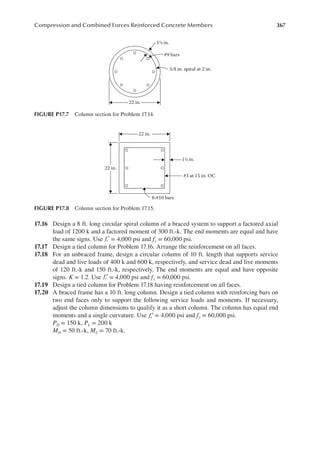
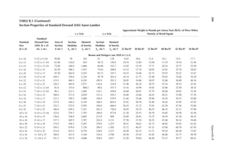
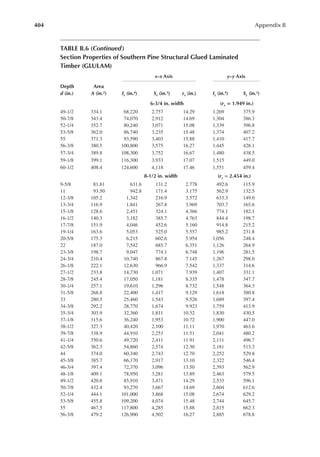
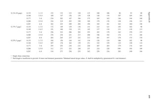
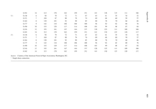
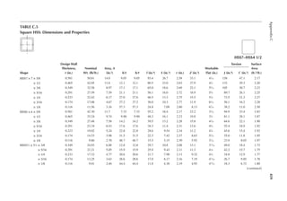
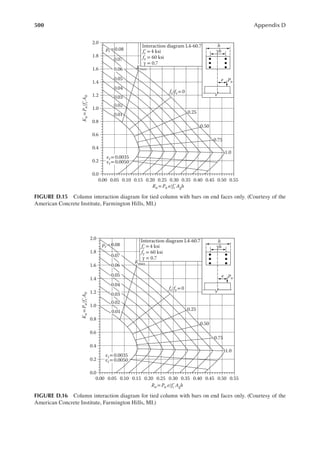
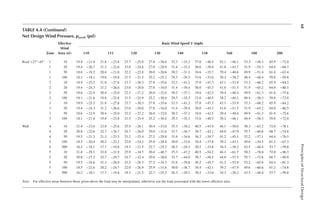
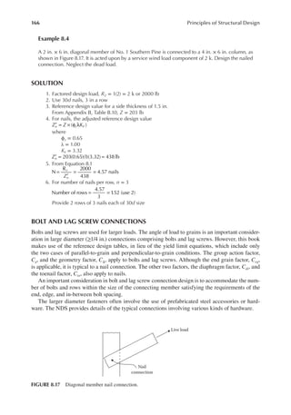
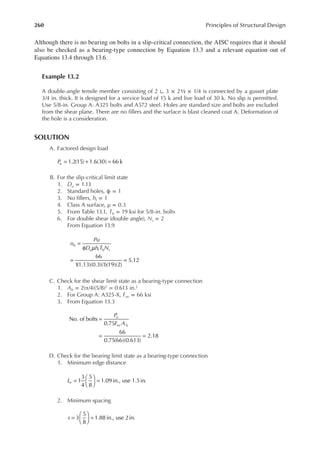
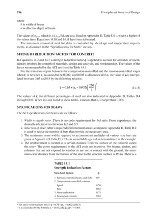
429. 411
Appendix B
TABLE B.9
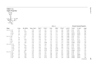
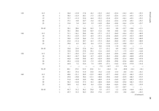
Reference Design Values for Structural Composite Lumber
Grade Orientation
Shear of
Elasticity
G (psi)
Modulus
of
Elasticity
e (psi)
Flexural
Stress
Fb
a (psi)
Tension
Stress
Ft
b (psi)
Compression
Perpendicular
to Grain Fc⊥
c (psi)
Compression
Parallel to
Grain Fc∥ (psi)
Horizontal Shear
Parallel to Grain
Fv (psi)
TimberStrand LSL
1.3E Beam/Column 81,250 1.3 × 106 3,140 1,985 1,240 2,235 745
Plank 81,250 1.3 × 106 3,510 790 2,235 280
1.55E Beam 96,875 1.55 × 106 4,295 1,975 1,455 3,270 575
Microllam LVL
1.9E Beam 118,750 1.9 × 106 4,805 2,870 1,365 4,005 530
Parallam PSL
1.8E 1.8 × 106
and 2.0E Column 112,500 2.0 × 106 4,435 3,245 775 3,990 355
2.0E Beam 125,000 2.0 × 106 5,360 3,750 1,365 4,630 540
a For 12-in. depth and for other depths, multiply, Fb, by the factors as follows: For TimberStrand LSL, multiply by [12/d]0.092; for Microllam
LVL, multiply by [12/d]0.136; for Parallam, PSL, multiply by [12/d]0.111.
b Ft has been adjusted to relect the volume effects for most standard applications.
c Fc┴
shall not be increased for duration of load.

430. 412
Appendix
B
TABLE B.10
Common Wire, Box, or Sinker Nails: Reference Lateral Design Values (Z) for Single-Shear (Two-Member) Connections
a
Side
Member
Thickness,
ts (in.)
Nail
Diameter,
D (in.)
Common
Wire Nail
Box
Nail
Sinker
Nail
G = 0.67,
Red Oak
(lb)
G = 0.55,
Mixed
Maple
Southern
Pine (lb)
G = 0.5,
Douglas
Fir-Larch
(lb)
G = 0.49,
Douglas
Fir-Larch
(North)
(lb)
G = 0.46,
Douglas Fir
(South)
Hem-Fir
(North) (lb)
G = 0.43,
Hem-Fir
(lb)
G = 0.42,
Spruce-
Pine-Fir
(lb)
G = 0.37,
Redwood
(Open
Grain) (lb)
G = 0.36, Eastern
Softwoods
Spruce-Pine-Fir
(South) Western
Cedars Western
Woods (lb)
G = 0.35,
Northern
Species (lb)
Pennyweight
3/4 0.099 6d 7d 73 61 55 54 51 48 47 39 38 36
0.113 6d 8d 8d 94 79 72 71 65 58 57 47 46 44
0.120 10d 107 89 80 77 71 64 62 52 50 48
0.128 10d 121 101 87 84 78 70 68 57 56 54
0.131 8d 127 104 90 87 80 73 70 60 58 56
0.135 16d 12d 135 108 94 91 84 76 74 63 61 58
0.148 10d 20d 16d 154 121 105 102 94 85 83 70 69 66
0.162 16d 40d 183 138 121 117 108 99 96 82 80 77
0.177 20d 200 153 134 130 121 111 107 92 90 87
0.192 20d 30d 206 157 138 134 125 114 111 96 93 90
0.207 30d 40d 216 166 147 143 133 122 119 103 101 97
0.225 40d 229 178 158 154 144 132 129 112 110 106
0.244 50d 60d 234 182 162 158 147 136 132 115 113 109
1 0.099 6d 7d 73 61 55 54 51 48 47 42 41 40
0.113 6db 8d 8d 94 79 72 71 67 63 61 55 54 51
0.120 10d 107 89 81 80 76 71 69 60 59 56
0.128 10d 121 101 93 91 86 80 79 66 64 61
0.131 8d 127 106 97 95 90 84 82 68 66 63
0.135 16d 12d 135 113 103 101 96 89 86 71 69 66
0.148 10d 20d 16d 154 128 118 115 109 99 96 80 77 74
0.162 16d 40d 184 154 141 137 125 113 109 91 89 85
0.177 20d 213 178 155 150 138 125 121 102 99 95
0.192 20d 30d 222 183 159 154 142 128 124 105 102 98
0.207 30d 40d 243 192 167 162 149 135 131 111 109 104

431. 413
Appendix
B
0.225 40d 268 202 177 171 159 144 140 120 117 112
0.244 50d 60d 274 207 181 175 162 148 143 123 120 115
1¼ 0.099 6d 7d 73 61 55 54 51 48 47 42 41 40
0.113 6d 8d 8d 94 79 72 71 67 63 61 55 54 52
0.120 10d 107 89 81 80 76 71 69 62 60 59
0.128 10d 121 101 93 91 86 80 79 70 69 67
0.131 8d 127 106 97 95 90 84 82 73 72 70
0.135 16d 12d 135 113 103 101 96 89 88 78 76 74
0.148 10d 20d 16d 154 128 118 115 109 102 100 89 87 84
0.162 16d 40d 184 154 141 138 131 122 120 103 100 95
0.177 20d 213 178 163 159 151 141 136 113 110 105
0.192 20d 30d 222 185 170 166 157 145 140 116 113 108
0.207 30d 40d 243 203 186 182 169 152 147 123 119 114
0.225 40d 268 224 200 193 177 160 155 130 127 121
0.244 50d 60d 276 230 204 197 181 163 158 133 129 124
1½ 0.099 7d 73 61 55 54 51 48 47 42 41 40
0.113 8d 8d 94 79 72 71 67 63 61 56 54 52
0.120 10d 107 89 81 80 76 71 69 62 60 59
0.128 10d 121 101 93 91 86 80 79 70 69 67
0.131 8d 127 106 97 95 90 84 82 73 72 70
0.135 16d 12d 135 113 103 101 96 89 88 78 76 74
0.148 10d 20d 16d 154 128 118 115 109 102 100 89 87 84
0.162 16d 40d 184 154 141 138 131 122 120 106 104 101
0.177 20d 213 178 163 159 151 141 138 123 121 117
0.192 20d 30d 222 185 170 166 157 147 144 128 126 120
0.207 30d 40d 243 203 186 182 172 161 158 135 131 125
0.225 40d 268 224 205 201 190 178 172 143 138 132
0.244 50d 60d 276 230 211 206 196 181 175 146 141 135
1¾ 0.113 8d 94 79 72 71 67 63 61 55 54 52
0.120 10d 107 89 81 80 76 71 69 62 60 59
0.128 10d 121 101 93 91 86 80 79 70 69 67
0.135 16d 12d 135 113 103 101 96 89 88 78 76 74
0.148 10d 20d 16d 154 128 118 115 109 102 100 89 87 84
0.162 16d 40d 184 154 141 138 131 122 120 106 104 101
0.177 20d 213 178 163 159 151 141 138 123 121 117
(Continued)

432. 414
Appendix
B
TABLE B.10 (continued)
Common Wire, Box, or Sinker Nails: Reference Lateral Design Values (Z) for Single-Shear (Two-Member) Connections
Side
Member
Thickness,
ts (in.)
Nail
Diameter,
D (in.)
Common
Wire Nail
Box
Nail
Sinker
Nail
G = 0.67,
Red Oak
(lb)
G = 0.55,
Mixed
Maple
Southern
Pine (lb)
G = 0.5,
Douglas
Fir-Larch
(lb)
G = 0.49,
Douglas
Fir-Larch
(North)
(lb)
G = 0.46,
Douglas Fir
(South)
Hem-Fir
(North) (lb)
G = 0.43,
Hem-Fir
(lb)
G = 0.42,
Spruce-
Pine-Fir
(lb)
G = 0.37,
Redwood
(Open
Grain) (lb)
G = 0.36, Eastern
Softwoods
Spruce-Pine-Fir
(South) Western
Cedars Western
Woods (lb)
G = 0.35,
Northern
Species (lb)
Pennyweight
0.192 20d 30d 222 185 170 166 157 147 144 128 126 122
0.207 30d 40d 243 203 186 182 172 161 158 140 137 133
0.225 40d 268 224 205 201 190 178 174 155 151 144
0.244 50d 60d 276 230 211 206 196 183 179 159 154 147
Source: Courtesy of the American Forest & Paper Association, Washington, DC.
a Single-shear connection.
b Italic d indicates that the nail length is insuficient to provide 10 times nail diameter penetration. Multiply the tabulated values by the ratio (penetration/10 × nail diameter).

433. 415
Appendix
B
TABLE B.11
Nail and Spike Reference Withdrawal Design Values (W)
Pounds per Inch of Nail Penetration
Common Wire Nails, Box Nails, and Common Wire Spikes Diameter, D Common Nails/Spikes, Box Nails Threaded Nails Wire Diameter, D
Speciic
gravity, G
0.099
in.
0.113
in.
0.128
in.
0.131
in.
0.135
in.
0.148
in.
0.162
in.
0.192
in.
0.207
in.
0.225
in.
0.244
in.
0.263
in.
0.283
in.
0.312
in.
0.375
in.
0.120
in.
0.135
in.
0.148
in.
0.177
in.
0.207
in.
0.73 62 71 80 82 85 93 102 121 130 141 153 165 178 196 236 82 93 102 121 141
0.71 58 66 75 77 79 87 95 113 121 132 143 154 166 183 220 77 87 95 113 132
0.68 52 59 67 69 71 78 85 101 109 118 128 138 149 164 197 69 78 85 101 118
0.67 50 57 65 66 68 75 82 97 105 114 124 133 144 158 190 66 75 82 97 114
0.58 35 40 45 46 48 52 57 68 73 80 86 93 100 110 133 46 52 57 68 80
0.55 31 35 40 41 42 46 50 59 64 70 76 81 88 97 116 41 46 50 59 70
0.51 25 29 33 34 35 38 42 49 53 58 63 67 73 80 96 34 38 42 49 58
0.50 24 28 31 32 33 36 40 47 50 55 60 64 69 76 91 32 36 40 47 55
0.49 23 26 30 30 31 34 38 45 48 52 57 61 66 72 87 30 34 38 45 52
0.47 21 24 27 27 28 31 34 40 43 47 51 55 59 65 78 27 31 34 40 47
0.46 20 22 25 26 27 29 32 38 41 45 48 52 56 62 74 26 29 32 38 45
0.44 18 20 23 23 24 26 29 34 37 40 43 47 50 55 66 23 26 29 34 40
0.43 17 19 21 22 23 25 27 32 35 38 41 44 47 52 63 22 25 27 32 38
0.42 16 18 20 21 21 23 26 30 33 35 38 41 45 49 59 21 23 26 30 35
0.41 15 17 19 19 20 22 24 29 31 33 36 39 42 46 56 19 22 24 29 33
0.40 14 16 18 18 19 21 23 27 29 31 34 37 40 44 52 18 21 23 27 31
0.39 13 15 17 17 18 19 21 25 27 29 32 34 37 41 49 17 19 21 25 29
0.38 12 14 16 16 17 18 20 24 25 28 30 32 35 38 46 16 18 20 24 28
0.37 11 13 15 15 16 17 19 22 24 26 28 30 33 36 43 15 17 19 22 26
0.36 11 12 14 14 14 16 17 21 22 24 26 28 30 33 40 14 16 17 21 24
0.35 10 11 13 13 14 15 16 19 21 23 24 26 28 31 38 13 15 16 19 23
0.31 7 8 9 10 10 11 12 14 15 17 18 19 21 23 28 10 11 12 14 17
Source: Courtesy of the American Forest & Paper Association, Washington, DC.

434. 416
Appendix
B
TABLE B.12
Post-Frame Ring Shank Nails: Reference Lateral Design Values, Z, for Single-Shear (Two-Member) Connections
a
Side Member
Thickness
Nail
Diameter Nail Length
G = 0.67,
Red Oak
G = 0.55,
Mixed
Maple,
Southern
Pine
G = 0.5,
Douglas
Fir-Larch
G = 0.49,
Douglas
Fir-Larch
(North)
G = 0.46,
Douglas
Fir (South),
Hem-Fir
(North)
G = 0.43,
Hem-Fir
G = 0.42,
Spruce-Pine-
Fir
G = 0.37,
Redwood
(Open Grain)
G = 0.36,
Eastern
Softwoods,
Spruce-Pine-
Fir (South),
Western
Cedars,
Western
Woods
G = 0.35,
Northern
Species
ts (in.) D (in.) L (in.) lb lb lb lb lb lb lb lb lb lb
1/2 0.135 3, 3.5 114 89 80 78 73 67 65 57 56 54
0.148 3–4.5 127 100 89 87 81 75 73 64 63 61
0.177 3–8 173 139 125 122 115 107 105 93 91 88
0.200 3.5–8 188 151 137 134 126 118 115 102 100 95
0.207 4–8 193 156 142 138 131 122 119 106 102 96
3/4 0.135 3, 3.5 138 106 93 90 83 75 73 62 61 58
0.148 3–4.5 156 118 103 100 92 84 81 70 68 65
0.177 3–8 204 157 139 134 125 115 112 97 94 91
0.200 3.5–8 218 168 149 145 135 124 121 105 103 99
0.207 4–8 223 173 153 149 139 128 125 109 106 103
1 0.135 3, 3.5 138 115 106 103 97 87 84 70 68 65
0.148 3–4.5 156 130 119 116 107 96 93 78 76 73
0.177 3–8 227 181 158 153 141 128 124 105 102 98
0.200 3.5–8 250 193 168 163 151 137 133 113 110 106
0.207 4–8 259 197 172 166 154 140 136 116 113 109
1¼ 0.135 3, 3.5 138 115 106 103 98 92 90 80 77 74
0.148 3–4.5 156 130 119 116 110 103 101 88 86 82
0.177 3–8 227 189 173 170 160 143 139 116 112 107

435. 417
Appendix
B
0.200 3.5–8 250 208 191 184 169 152 147 123 120 115
0.207 4–8 259 216 195 188 172 155 150 126 123 118
1½ 0.135 3, 3.5 138 115 106 103 98 92 90 80 78 76
0.148 3–4.5 156 130 119 116 110 103 101 90 88 85
0.177 3–8 227 189 173 170 161 150 147 128 124 118
0.200 3.5–8 250 208 191 187 177 166 162 136 132 126
0.207 4–8 259 216 198 194 184 172 167 139 134 128
1¾ 0.135 3, 3.5 138 115 106 103 98 92 90 80 78 76
0.148 3–4.5 156 130 119 116 110 103 101 90 88 85
0.177 3b, 3.5b, 4–8 227 189 173 170 161 150 147 131 128 125
0.200 3.5b, 4–8 250 208 191 187 177 166 162 144 141 137
0.207 4–8 259 216 198 194 184 172 168 149 147 140
2½ 0.135 3.5b 138 115 106 103 98 92 90 80 78 76
0.148 3.5b, 4, 4.5 156 130 119 116 110 103 101 90 88 85
0.177 4b, 4.5, 5, 6, 8 227 189 173 170 161 150 147 131 128 125
0.200 4b, 4.5, 5, 6, 8 250 208 191 187 177 166 162 144 141 137
0.207 4b, 4.5b, 5, 6, 8 259 216 198 194 184 172 168 149 147 142
3½ 0.148 4.5b 156 130 119 116 110 103 101 90 88 85
0.177 5b, 6, 8 227 189 173 170 161 150 147 131 128 125
0.200 5b, 6, 8 250 208 191 187 177 166 162 144 141 137
0.207 5b, 6, 8 259 216 198 194 184 172 168 149 147 142
0.036 (20 gage) 0.135 3, 3.5 130 111 102 100 95 89 88 78 77 75
0.148 3–4.5 142 125 115 113 107 101 99 88 87 84
0.177 3–8 171 171 167 164 156 146 143 128 126 122
0.200 3.5–8 177 177 177 177 172 161 158 141 139 135
0.207 4–8 178 178 178 178 178 167 164 146 144 140
0.048 (18 gage) 0.135 3, 3.5 131 111 103 101 96 90 88 79 78 76
0.148 3–4.5 147 125 116 113 108 101 99 89 87 85
0.177 3–8 213 182 168 164 156 147 144 129 127 123
0.200 3.5–8 235 200 184 181 172 162 158 142 139 135
0.207 4–8 237 207 191 187 178 168 164 147 144 140
(Continued)

436. 418
Appendix
B
TABLE B.12 (continued)
Post-Frame Ring Shank Nails: Reference Lateral Design Values, Z, for Single-Shear (Two-Member) Connections
Side Member
Thickness
Nail
Diameter Nail Length
G = 0.67,
Red Oak
G = 0.55,
Mixed
Maple,
Southern
Pine
G = 0.5,
Douglas
Fir-Larch
G = 0.49,
Douglas
Fir-Larch
(North)
G = 0.46,
Douglas
Fir (South),
Hem-Fir
(North)
G = 0.43,
Hem-Fir
G = 0.42,
Spruce-Pine-
Fir
G = 0.37,
Redwood
(Open Grain)
G = 0.36,
Eastern
Softwoods,
Spruce-Pine-
Fir (South),
Western
Cedars,
Western
Woods
G = 0.35,
Northern
Species
ts (in.) D (in.) L (in.) lb lb lb lb lb lb lb lb lb lb
0.060 (16 gage) 0.135 3, 3.5 132 113 104 102 97 92 90 81 79 77
0.148 3–4.5 148 126 117 115 109 103 101 90 89 86
0.177 3–8 214 183 169 165 157 148 145 130 128 124
0.200 3.5–8 235 201 185 182 173 163 159 143 140 136
0.207 4–8 244 208 192 188 179 168 165 148 145 141
0.075 (14 gage) 0.135 3, 3.5 134 115 106 104 100 94 92 83 81 79
0.148 3–4.5 150 129 119 117 112 105 103 93 91 88
0.177 3–8 216 185 171 167 160 150 147 132 130 126
0.200 3.5–8 237 203 187 183 175 164 161 145 142 138
0.207 4–8 246 210 194 190 181 170 167 150 147 143
0.105 (12 gage) 0.135 3, 3.5 142 122 113 111 106 100 98 88 87 83
0.148 3–4.5 159 137 127 124 119 112 110 99 97 94
0.177 3–8 223 192 178 174 166 157 154 138 136 132
0.200 3.5–8 244 209 194 190 181 171 167 150 148 144
0.207 4–8 252 216 200 196 187 176 173 155 153 148
0.120 (11 gage) 0.135 3, 3.5 147 127 118 115 110 104 102 92 90 86
0.148 3–4.5 164 141 131 129 123 116 114 103 101 98
0.177 3–8 228 197 182 179 171 161 158 142 140 136
0.200 3.5–8 249 214 198 194 185 175 171 154 152 147
0.207 4–8 257 221 204 200 191 180 177 159 156 152

437. 419
Appendix
B
0.134 (10 gage) 0.135 3, 3.5 152 132 122 120 115 108 106 96 93 88
0.148 3–4.5 169 147 136 134 128 120 118 107 105 102
0.177 3–8 234 202 187 184 175 165 162 146 144 140
0.200 3.5–8 254 219 203 199 190 179 176 158 156 151
0.207 4–8 262 225 209 205 196 185 181 163 160 156
0.179 (7 gage) 0.135 3, 3.5 172 149 139 136 131 123 121 105 102 98
0.148 3–4.5 191 166 154 151 145 137 134 121 118 113
0.177 3–8 256 222 206 202 193 183 179 162 159 153
0.200 3.5–8 276 238 221 217 208 196 192 174 171 166
0.207 4–8 283 245 227 223 213 201 197 178 175 170
0.239 (3 gage) 0.135 3, 3.5 184 156 144 141 134 126 124 106 102 98
0.148 3–4.5 207 176 162 159 151 142 139 124 120 114
0.177 3–8 293 255 236 232 220 207 203 179 174 165
0.200 3.5–8 312 271 252 248 237 224 220 199a 195 189
0.207 4–8 319 277 258 253 242 229 224 203 199 194
a Single shear connection.
b Nail length is insuficient to provide 10 times nail diameter penetration. Tabulated lateral design values, Z, shall be multiplied by (penetration/10 × nail diameter).

438. 420 Appendix B
TABLE B.13
Post-Frame Ring Shank Nail Reference Withdrawal
Design Values, W, Pounds per Inch of Ring Shank
Penetration into Side Grain of Wood Member
Speciic
Gravity, G
Diameter, D (in.)
0.135 0.148 0.177 0.200 0.207
0.73 129 142 170 192 199
0.71 122 134 161 181 188
0.68 112 123 147 166 172
0.67 109 120 143 162 167
0.58 82 90 107 121 125
0.55 74 81 96 109 113
0.51 63 69 83 94 97
0.50 61 67 80 90 93
0.49 58 64 76 86 89
0.47 54 59 70 80 82
0.46 51 56 67 76 79
0.44 47 52 62 70 72
0.43 45 49 59 67 69
0.42 43 47 56 64 66
0.41 41 45 54 61 63
0.40 39 43 51 58 60
0.39 37 41 48 55 57
0.38 35 38 46 52 54
0.37 33 36 44 49 51
0.36 31 35 41 47 48
0.35 30 33 39 44 46
0.31 23 26 31 35 36

439. 421
Appendix
B
TABLE B.14
Wood Screws: Reference Lateral Design Values (Z) for Single-Shear (Two-Member) Connections
a
Side
Member
Thickness,
ts (in.)
Wood
Screw
Diameter,
D (in.)
Wood
Screw
Number
G = 0.67,
Red Oak
(lb)
G = 0.55,
Mixed
Maple
Southern
Pine (lb)
G = 0.5,
Douglas
Fir-Larch
(lb)
G = 0.49,
Douglas
Fir-Larch
(North)
(lb)
G = 0.46,
Douglas
Fir
(South)
Hem-Fir
(North)
(lb)
G =
0.43,
Hem-Fir
(lb)
G = 0.42,
Spruce-
Pine-Fir
(lb)
G = 0.37,
Redwood
(Open
Grain)
(lb)
G = 0.36,
Eastern
Softwoods
Spruce-
Pine-Fir
(South)
Western
Cedars
Western
Woods (lb)
G = 0.35,
Northern
Species (lb)
1/2 0.138 6 88 67 59 57 53 49 47 41 40 38
0.151 7 96 74 65 63 59 54 52 45 44 42
0.164 8 107 82 73 71 66 61 59 51 50 48
0.177 9 121 94 83 81 76 70 68 59 58 56
0.190 10 130 101 90 87 82 75 73 64 63 60
0.216 12 156 123 110 107 100 93 91 79 78 75
0.242 14 168 133 120 117 110 102 99 87 86 83
5/8 0.138 6 94 76 66 64 59 53 52 44 43 41
0.151 7 104 83 72 70 64 58 56 48 47 45
0.164 8 120 92 80 77 72 65 63 54 53 51
0.177 9 136 103 91 88 81 74 72 62 61 58
0.190 10 146 111 97 94 88 80 78 67 65 63
0.216 12 173 133 117 114 106 97 95 82 80 77
0.242 14 184 142 126 123 115 106 103 89 87 84
3/4 0.138 6 94 79 72 71 65 58 57 47 46 44
0.151 7 104 87 80 77 71 64 62 52 50 48
0.164 8 120 101 88 85 78 71 69 58 56 54
(Continued)

440. 422
Appendix
B
TABLE B.14 (continued)
Wood Screws: Reference Lateral Design Values (Z) for Single-Shear (Two-Member) Connections
Side
Member
Thickness,
ts (in.)
Wood
Screw
Diameter,
D (in.)
Wood
Screw
Number
G = 0.67,
Red Oak
(lb)
G = 0.55,
Mixed
Maple
Southern
Pine (lb)
G = 0.5,
Douglas
Fir-Larch
(lb)
G = 0.49,
Douglas
Fir-Larch
(North)
(lb)
G = 0.46,
Douglas
Fir
(South)
Hem-Fir
(North)
(lb)
G =
0.43,
Hem-Fir
(lb)
G = 0.42,
Spruce-
Pine-Fir
(lb)
G = 0.37,
Redwood
(Open
Grain)
(lb)
G = 0.36,
Eastern
Softwoods
Spruce-
Pine-Fir
(South)
Western
Cedars
Western
Woods (lb)
G = 0.35,
Northern
Species (lb)
0.177 9 142 114 99 96 88 80 78 66 64 61
0.190 10 153 122 107 103 95 86 83 71 69 66
0.216 12 192 144 126 122 113 103 100 86 84 80
0.242 14 203 154 135 131 122 111 108 93 91 87
1 0.138 6 94 79 72 71 67 63 61 55 54 51
0.151 7 104 87 80 78 74 69 68 60 59 56
0.164 8 120 101 92 90 85 80 78 67 65 62
0.177 9 142 118 108 106 100 94 90 75 73 70
0.190 10 153 128 117 114 108 101 97 81 78 75
0.216 12 193 161 147 143 131 118 114 96 93 89
0.242 14 213 178 157 152 139 126 122 102 100 95
11
⁄4 0.138 6 94 79 72 71 67 63 61 55 54 52
0.151 7 104 87 80 78 74 69 68 60 59 57
0.164 8 120 101 92 90 85 80 78 70 68 66
0.177 9 142 118 108 106 100 94 92 82 80 78
0.190 10 153 128 117 114 108 101 99 88 87 84
0.216 12 193 161 147 144 137 128 125 108 105 100

441. 423
Appendix
B
0.242 14 213 178 163 159 151 141 138 115 111 106
11
⁄2 0.138 6 94 79 72 71 67 63 61 55 54 52
0.151 7 104 87 80 78 74 69 68 60 59 57
0.164 8 120 101 92 90 85 80 78 70 68 66
0.177 9 142 118 108 106 100 94 92 82 80 78
0.190 10 153 128 117 114 108 101 99 88 87 84
0.216 12 193 161 147 144 137 128 125 111 109 106
0.242 14 213 178 163 159 151 141 138 123 120 117
13
⁄4 0.138 6 94 79 72 71 67 63 61 55 54 52
0.151 7 104 87 80 78 74 69 68 60 59 57
0.164 8 120 101 92 90 85 80 78 70 68 66
0.177 9 142 118 108 106 100 94 92 82 80 78
0.190 10 153 128 117 114 108 101 99 88 87 84
0.216 12 193 161 147 144 137 128 125 111 109 106
0.242 14 213 178 163 159 151 141 138 123 120 117
Source: Courtesy of the American Forest & Paper Association, Washington, DC.
a Single-shear connection.

442. 424 Appendix B
TABLE B.15
Cut Thread or Rolled Thread Wood Screw Reference Withdrawal Design Values (W)
Pounds per Inch of Thread Penetration
Speciic
Gravity, G
Wood Screw Number
6 7 8 9 10 12 14 16 18 20 24
0.73 209 229 249 268 288 327 367 406 446 485 564
0.71 198 216 235 254 272 310 347 384 421 459 533
0.68 181 199 216 233 250 284 318 352 387 421 489
0.67 176 193 209 226 243 276 309 342 375 409 475
0.58 132 144 157 169 182 207 232 256 281 306 356
0.55 119 130 141 152 163 186 208 231 253 275 320
0.51 102 112 121 131 141 160 179 198 217 237 275
0.50 98 107 117 126 135 154 172 191 209 228 264
0.49 94 103 112 121 130 147 165 183 201 219 254
0.47 87 95 103 111 119 136 152 168 185 201 234
0.46 83 91 99 107 114 130 146 161 177 193 224
0.44 76 83 90 97 105 119 133 148 162 176 205
0.43 73 79 86 93 100 114 127 141 155 168 196
0.42 69 76 82 89 95 108 121 134 147 161 187
0.41 66 72 78 85 91 103 116 128 141 153 178
0.40 63 69 75 81 86 98 110 122 134 146 169
0.39 60 65 71 77 82 93 105 116 127 138 161
0.38 57 62 67 73 78 89 99 110 121 131 153
0.37 54 59 64 69 74 84 94 104 114 125 145
0.36 51 56 60 65 70 80 89 99 108 118 137
0.35 48 53 57 62 66 75 84 93 102 111 130
0.31 38 41 45 48 52 59 66 73 80 87 102
Source: Courtesy of the American Forest & Paper Association, Washington, DC.
Note: Tabulated withdrawal design values (W) are in pounds per inch of thread penetration into side grain of main
member. Thread length is approximately two-thirds the total wood screw length.

443. 425
Appendix
B
TABLE B.16
Bolts: Reference Lateral Design Values (Z) for Single-Shear (Two-Member) Connections
a
Thickness G = 0.67, Red Oak
G = 0.55, Mixed Maple
Southern Pine G = 0.50, Douglas Fir-Larch
G = 0.49, Douglas Fir-Larch
(North)
G = 0.46, Douglas Fir
(South) Hem-Fir (North)
Main
member,
tm (in.)
Side
member,
ts (in.)
Bolt
diameter,
D (in.)
Z∥
(lb)
Zs⊥
(lb)
Zm⊥
(lb)
Z⊥
(lb)
Z∥
(lb)
Zs⊥
(lb)
Zm⊥
(lb)
Z⊥
(lb)
Z∥
(lb)
Zs⊥
(lb)
Zm⊥
(lb)
Z⊥
(lb)
Z∥
(lb)
Zs⊥
(lb)
Zm⊥
(lb)
Z⊥
(lb)
Z∥
(lb)
Zs⊥
(lb)
Zm⊥
(lb)
Z⊥
(lb)
11
⁄2 11
⁄2 1/2 650 420 420 330 530 330 330 250 480 300 300 220 470 290 290 210 440 270 270 190
5/8 810 500 500 370 660 400 400 280 600 360 360 240 590 350 350 240 560 320 320 220
3/4 970 580 580 410 800 460 460 310 720 420 420 270 710 400 400 260 670 380 380 240
7/8 1130 660 660 440 930 520 520 330 850 470 470 290 830 460 460 280 780 420 420 250
1 1290 740 740 470 1060 580 580 350 970 530 530 310 950 510 510 300 890 480 480 280
13
⁄4 13
⁄4 1/2 760 490 490 390 620 390 390 290 560 350 350 250 550 340 340 250 520 320 320 230
5/8 940 590 590 430 770 470 470 330 700 420 420 280 690 410 410 280 650 380 380 250
3/4 1130 680 680 480 930 540 540 360 850 480 480 310 830 470 470 300 780 440 440 280
7/8 1320 770 770 510 1080 610 610 390 990 550 550 340 970 530 530 320 910 500 500 300
1 1510 860 860 550 1240 680 680 410 1130 610 610 360 1110 600 600 350 1040 560 560 320
21
⁄2 11
⁄2 1/2 770 480 540 440 660 400 420 350 610 370 370 310 610 360 360 300 580 340 330 270
5/8 1070 660 630 520 930 560 490 390 850 520 430 340 830 520 420 330 780 470 390 300
3/4 1360 890 720 570 1120 660 560 430 1020 590 500 380 1000 560 480 360 940 520 450 330
7/8 1590 960 800 620 1300 720 620 470 1190 630 550 410 1170 600 540 390 1090 550 500 360
1 1820 1020 870 660 1490 770 680 490 1360 680 610 440 1330 650 590 420 1250 600 550 390
31
⁄2 11
⁄2 1/2 770 480 560 440 660 400 470 360 610 370 430 330 610 360 420 320 580 340 400 310
5/8 1070 660 760 590 940 560 620 500 880 520 540 460 870 520 530 450 830 470 490 410
3/4 1450 890 900 770 1270 660 690 580 1200 590 610 510 1190 560 590 490 1140 520 550 450
7/8 1890 960 990 830 1680 720 770 630 1590 630 680 550 1570 600 650 530 1470 550 600 480
1 2410 1020 1080 890 2010 770 830 670 1830 680 740 590 1790 650 710 560 1680 600 660 520
3½ 1¾ 1/2 830 510 590 480 720 420 510 390 670 380 470 350 660 380 460 340 620 360 440 320
5/8 1160 680 820 620 1000 580 640 520 930 530 560 460 920 530 550 450 880 500 510 410
3/4 1530 900 940 780 1330 770 720 580 1250 680 640 520 1240 660 620 500 1190 600 580 460
(Continued)

444. 426
Appendix
B
TABLE B.16 (continued)
Bolts: Reference Lateral Design Values (Z) for Single-Shear (Two-Member) Connections
Thickness G = 0.67, Red Oak
G = 0.55, Mixed Maple
Southern Pine G = 0.50, Douglas Fir-Larch
G = 0.49, Douglas Fir-Larch
(North)
G = 0.46, Douglas Fir
(South) Hem-Fir (North)
Main
member,
tm (in.)
Side
member,
ts (in.)
Bolt
diameter,
D (in.)
Z∥
(lb)
Zs⊥
(lb)
Zm⊥
(lb)
Z⊥
(lb)
Z∥
(lb)
Zs⊥
(lb)
Zm⊥
(lb)
Z⊥
(lb)
Z∥
(lb)
Zs⊥
(lb)
Zm⊥
(lb)
Z⊥
(lb)
Z∥
(lb)
Zs⊥
(lb)
Zm⊥
(lb)
Z⊥
(lb)
Z∥
(lb)
Zs⊥
(lb)
Zm⊥
(lb)
Z⊥
(lb)
7/8 1970 1120 1040 840 1730 840 810 640 1620 740 710 550 1590 700 690 530 1490 640 640 490
1 2480 1190 1130 900 2030 890 880 670 1850 790 780 590 1820 750 760 570 1700 700 700 530
31
⁄2 31
⁄2 1/2 830 590 590 530 750 520 520 460 720 490 490 430 710 480 480 420 690 460 460 410
5/8 1290 880 880 780 1170 780 780 650 1120 700 700 560 1110 690 690 550 1070 650 650 500
3/4 1860 1190 1190 950 1690 960 960 710 1610 870 870 630 1600 850 850 600 1540 800 800 560
7/8 2540 1410 1410 1030 2170 1160 1160 780 1970 1060 1060 680 1940 1040 1040 650 1810 980 980 590
1 3020 1670 1670 1100 2480 1360 1360 820 2260 1230 1230 720 2210 1190 1190 690 2070 1110 1110 640
51
⁄4 11
⁄2 5/8 1070 660 760 590 940 560 640 500 880 520 590 460 870 520 590 450 830 470 560 430
3/4 1450 890 990 780 1270 660 850 660 1200 590 790 590 1190 560 780 560 1140 520 740 520
7/8 1890 960 1260 960 1680 720 1060 720 1590 630 940 630 1570 600 900 600 1520 550 830 550
1 2410 1020 1500 1020 2150 770 1140 770 2050 680 1010 680 2030 650 970 650 1930 600 910 600
51
⁄4 13
⁄4 5/8 1160 680 820 620 1000 580 690 520 930 530 630 470 920 530 630 470 880 500 590 440
3/4 1530 900 1050 800 1330 770 890 680 1250 680 830 630 1240 660 810 620 1190 600 780 590
7/8 1970 1120 1320 1020 1730 840 1090 840 1640 740 960 740 1620 700 920 700 1550 640 850 640
1 2480 1190 1530 1190 2200 890 1170 890 2080 790 1040 790 2060 750 1000 750 1990 700 930 700
51
⁄4 31
⁄2 5/8 1290 880 880 780 1170 780 780 680 1120 700 730 630 1110 690 720 620 1070 650 690 580
3/4 1860 1190 1240 1080 1690 960 1090 850 1610 870 1030 780 1600 850 1010 750 1540 800 970 710
7/8 2540 1410 1640 1260 2300 1160 1380 1000 2190 1060 1230 870 2170 1040 1190 840 2060 980 1100 770
1 3310 1670 1940 1420 2870 1390 1520 1060 2660 1290 1360 940 2630 1260 1320 900 2500 1210 1230 830
51
⁄2 11
⁄2 5/8 1070 660 760 590 940 560 640 500 880 520 590 460 870 520 590 450 830 470 560 430
3/4 1450 890 990 780 1270 660 850 660 1200 590 790 590 1190 560 780 560 1140 520 740 520
7/8 1890 960 1260 960 1680 720 1090 720 1590 630 980 630 1570 600 940 600 1520 550 860 550
1 2410 1020 1560 1020 2150 770 1190 770 2050 680 1060 680 2030 650 1010 650 1930 600 940 600

445. 427
Appendix
B
51
⁄2 31
⁄2 5/8 1290 880 880 780 1170 780 780 680 1120 700 730 630 1110 690 720 620 1070 650 690 580
3/4 1860 1190 1240 1080 1690 960 1090 850 1610 870 1030 780 1600 850 1010 750 1540 800 970 710
7/8 2540 1410 1640 1260 2300 1160 1410 1020 2190 1060 1260 910 2170 1040 1220 870 2060 980 1130 790
1 3310 1670 1980 1470 2870 1390 1550 1100 2660 1290 1390 970 2630 1260 1340 930 2500 1210 1250 860
71
⁄2 11
⁄2 5/8 1070 660 760 590 940 560 640 500 880 520 590 460 870 520 590 450 830 470 560 430
3/4 1450 890 990 780 1270 660 850 660 1200 590 790 590 1190 560 780 560 1140 520 740 520
7/8 1890 960 1260 960 1680 720 1090 720 1590 630 1010 630 1570 600 990 600 1520 550 950 550
1 2410 1020 1560 1020 2150 770 1350 770 2050 680 1270 680 2030 650 1240 650 1930 600 1190 600
71
⁄2 31
⁄2 5/8 1290 880 880 780 1170 780 780 680 1120 700 730 630 1110 690 720 620 1070 650 690 580
3/4 1860 1190 1240 1080 1690 960 1090 850 1610 870 1030 780 1600 850 1010 750 1540 800 970 710
7/8 2540 1410 1640 1260 2300 1160 1450 1020 2190 1060 1360 930 2170 1040 1340 900 2060 980 1280 850
1 3310 1670 2090 1470 2870 1390 1830 1210 2660 1290 1630 1110 2630 1260 1570 1080 2500 1210 1470 1030
Source: Courtesy of the American Forest & Paper Association, Washington, DC.
a Single-shear connection.

446. 428
Appendix
B
TABLE B.17
Lag Screws: Reference Lateral Design Values (Z) for Single-Shear (Two-Member) Connections
a
Side
Member
Thickness,
ts (in.)
Lag Screw
Diameter,
D (in.)
G = 0.67, Red Oak
G = 0.55, Mixed Maple
Southern Pine G = 0.50, Douglas Fir-Larch
G = 0.49, Douglas Fir-Larch
(North)
G = 0.46, Douglas Fir
(South) Hem-Fir (North)
Z∥
(lb)
Zs⊥
(lb)
Zm⊥
(lb)
Z⊥
(lb)
Z∥
(lb)
Zs⊥
(lb)
Zm⊥
(lb)
Z⊥
(lb)
Z∥
(lb)
Zs⊥
(lb)
Zm⊥
(lb)
Z⊥
(lb)
Z∥
(lb)
Zs⊥
(lb)
Zm⊥
(lb)
Z⊥
(lb)
Z∥
(lb)
Zs⊥
(lb)
Zm⊥
(lb)
Z⊥
(lb)
1/2 1/4 150 110 110 110 130 90 100 90 120 90 90 80 120 90 90 80 110 80 90 80
5/16 170 130 130 120 150 110 120 100 150 100 110 100 140 100 110 90 140 100 100 90
3/8 180 130 130 120 160 110 110 100 150 100 110 90 150 90 110 90 140 90 100 90
5/8 1/4 160 120 130 120 140 100 110 100 130 90 100 90 130 90 100 90 120 90 90 80
5/16 190 140 140 130 160 110 120 110 150 110 110 100 150 100 110 100 150 100 110 90
3/8 190 130 140 120 170 110 120 100 160 100 110 100 160 100 110 90 150 100 110 90
3/4 1/4 180 140 140 130 150 110 120 110 140 100 110 100 140 100 110 90 130 90 100 90
5/16 210 150 160 140 180 120 130 120 170 110 120 100 160 110 120 100 160 100 110 100
3/8 210 140 160 130 180 120 130 110 170 110 120 100 170 110 120 100 160 100 110 90
1 1/4 180 140 140 140 160 120 120 120 150 120 120 110 150 110 110 110 150 110 110 100
5/16 230 170 170 160 210 140 150 130 190 130 140 120 190 120 140 120 180 120 130 110
3/8 230 160 170 160 210 130 150 120 200 120 140 110 190 120 140 110 180 110 130 100
11
⁄4 1/4 180 140 140 140 160 120 120 120 150 120 120 110 150 110 110 110 150 110 110 100
5/16 230 170 170 160 210 150 150 140 200 140 140 130 200 140 140 130 190 130 140 120
3/8 230 170 170 160 210 150 150 140 200 140 140 130 200 130 140 120 190 120 140 120
11
⁄2 1/4 180 140 140 140 160 120 120 120 150 120 120 110 150 110 110 110 150 110 110 100
5/16 230 170 170 160 210 150 150 140 200 140 140 130 200 140 140 130 190 140 140 130
3/8 230 170 170 160 210 150 150 140 200 140 140 130 200 140 140 130 190 140 140 120
7/16 360 260 260 240 320 220 230 200 310 200 210 180 310 190 210 180 300 180 200 160
1/2 460 310 320 280 410 250 290 230 390 220 270 200 390 220 260 200 370 210 250 190
5/8 700 410 500 370 600 340 420 310 560 310 380 280 550 310 380 270 530 290 360 260
3/4 950 550 660 490 830 470 560 410 770 440 510 380 760 430 510 370 730 400 480 360
7/8 1240 720 830 630 1080 560 710 540 1020 490 660 490 1010 470 650 470 970 430 610 430
1 1550 800 1010 780 1360 600 870 600 1290 530 810 530 1280 500 790 500 1230 470 760 470
13
⁄4 1/4 180 140 140 140 160 120 120 120 150 120 120 110 150 110 110 110 150 110 110 100

447. 429
Appendix
B
5/16 230 170 170 160 210 150 150 140 200 140 140 130 200 140 140 130 190 140 140 130
3/8 230 170 170 160 210 150 150 140 200 140 140 130 200 140 140 130 190 140 140 120
7/16 360 260 260 240 320 230 230 210 310 210 210 190 310 210 210 190 300 200 200 180
1/2 460 320 320 290 410 270 290 250 390 240 270 220 390 240 260 220 380 220 250 200
5/8 740 440 500 400 660 360 440 320 610 330 420 290 600 320 410 290 570 300 390 270
3/4 1030 580 720 520 890 480 600 430 830 450 550 390 820 440 540 380 780 420 510 360
7/8 1320 740 890 650 1150 630 750 550 1070 570 700 510 1060 550 680 490 1010 500 650 470
1 1630 910 1070 790 1420 700 910 670 1340 610 850 610 1320 590 830 590 1270 550 790 550
21
⁄2 1/4 180 140 140 140 160 120 120 120 150 120 120 110 150 110 110 110 150 110 110 100
5/16 230 170 170 160 210 150 150 140 200 140 140 130 200 140 140 130 190 140 140 130
3/8 230 170 170 160 210 150 150 140 200 140 140 130 200 140 140 130 190 140 140 120
7/16 360 260 260 240 320 230 230 210 310 210 210 190 310 210 210 190 300 200 200 180
1/2 460 320 320 290 410 290 290 250 390 270 270 240 390 260 260 230 380 250 250 220
5/8 740 500 500 450 670 430 440 390 640 390 420 350 630 380 410 340 610 360 390 320
3/4 1110 680 740 610 1010 550 650 490 960 500 610 450 950 490 600 430 920 460 580 410
7/8 1550 830 1000 740 1370 690 880 600 1280 630 830 550 1260 620 810 530 1190 580 770 500
1 1940 980 1270 860 1660 830 1080 720 1550 770 990 660 1520 750 970 640 1450 720 920 620
31
⁄2 1/4 180 140 140 140 160 120 120 120 150 120 120 110 150 110 110 110 150 110 110 100
5/16 230 170 170 160 210 150 150 140 200 140 140 130 200 140 140 130 190 140 140 130
3/8 230 170 170 160 210 150 150 140 200 140 140 130 200 140 140 130 190 140 140 120
7/16 360 260 260 240 320 230 230 210 310 210 210 190 310 210 210 190 300 200 200 180
1/2 460 320 320 290 410 290 290 250 390 270 270 240 390 260 260 230 380 250 250 220
5/8 740 500 500 450 670 440 440 390 640 420 420 360 630 410 410 360 610 390 390 340
3/4 1110 740 740 650 1010 650 650 560 960 600 610 520 950 580 600 510 920 550 580 490
7/8 1550 990 1000 860 1400 800 880 710 1340 720 830 640 1320 700 810 620 1280 660 780 570
1 2020 1140 1270 1010 1830 930 1120 810 1740 850 1060 740 1730 830 1040 720 1670 790 1000 680
Source: Courtesy of the American Forest & Paper Association, Washington, DC.
a Single-shear connection.

448. 430
Appendix
B
TABLE B.18
Lag Screw Reference Withdrawal Design Values (W)
Pounds per Inch of Thread Penetration
Lag Screw Unthreaded Shank Diameter, D
Speciic
Gravity, G 1/4 in. 5/16 in. 3/8 in. 7/16 in. 1/2 in. 5/8 in. 3/4 in. 7/8 in. 1 in. 1 1/8 in. 1 1/4 in.
0.73 397 469 538 604 668 789 905 1016 1123 1226 1327
0.71 381 450 516 579 640 757 868 974 1077 1176 1273
0.68 357 422 484 543 600 709 813 913 1009 1103 1193
0.67 349 413 473 531 587 694 796 893 987 1078 1167
0.58 281 332 381 428 473 559 641 719 795 869 940
0.55 260 307 352 395 437 516 592 664 734 802 868
0.51 232 274 314 353 390 461 528 593 656 716 775
0.50 225 266 305 342 378 447 513 576 636 695 752
0.49 218 258 296 332 367 434 498 559 617 674 730
0.47 205 242 278 312 345 408 467 525 580 634 686
0.46 199 235 269 302 334 395 453 508 562 613 664
0.44 186 220 252 283 312 369 423 475 525 574 621
0.43 179 212 243 273 302 357 409 459 508 554 600
0.42 173 205 235 264 291 344 395 443 490 535 579
0.41 167 198 226 254 281 332 381 428 473 516 559
0.40 161 190 218 245 271 320 367 412 455 497 538
0.39 155 183 210 236 261 308 353 397 438 479 518
0.38 149 176 202 227 251 296 340 381 422 461 498
0.37 143 169 194 218 241 285 326 367 405 443 479
0.36 137 163 186 209 231 273 313 352 389 425 460
0.35 132 156 179 200 222 262 300 337 373 407 441
0.31 110 130 149 167 185 218 250 281 311 339 367
Source: Courtesy of the American Forrest and Paper Association, Washington, DC.
Notes: Tabulated withdrawal design values (W) are in pounds per inch of thread penetration into side grain of main member. Length of thread
penetration in main member shall not include the length of the tapered tip.

449. 431
Appendix C: Steel

450. 432
Appendix
C
TABLE C.1a
W Shapes: Dimensions
tf k1
bf
tw
k
k
T
d
Y
Y
X
X
Shape
Area,
A (in.2)
Depth,
d (in.)
Web Flange Distance
Thickness, tw (in.)
2
(in.)
tw
Width, bf (in.) Thickness, tf (in.)
k
k1 (in.) t (in.)
Workable
Gage (in.)
kdes (in.) kdet (in.)
W21 × 93 27.3 21.6 215
⁄8 0.580 9/16 5/16 8.42 83
⁄8 0.930 15/16 1.43 15
⁄8 15/16 183
⁄8 51
⁄2
× 83a 24.4 21.4 213
⁄8 0.515 1/2 1/4 8.36 83
⁄6 0.835 13/16 1.34 11
⁄2 7/8
× 73a 21.5 21.2 211
⁄4 0.455 7/16 1/4 8.30 81
⁄4 0.740 3/4 1.24 17
⁄16 7/8
× 68a 20.0 21.1 211
⁄8 0.430 7/16 1/4 8.27 81
⁄4 0.685 11/16 1.19 13
⁄8 7/8
× 62a 18.3 21.0 21 0.400 3/8 3/16 8.24 81
⁄4 0.615 5/8 1.12 15
⁄16 13/16
× 55a 16.2 20.8 203
⁄4 0.375 3/8 3/16 8.22 81
⁄4 0.522 1/2 1.02 13
⁄16 13/16
× 48a,b 14.1 20.6 205
⁄8 0.350 3/8 3/16 8.14 81
⁄8 0.430 7/16 0.930 11
⁄8 13/16
W21 × 57a 16.7 21.1 21 0.405 3/8 3/16 6.56 61
⁄2 0.650 5/8 1.15 15
⁄16 13/16 183
⁄8 31
⁄2
× 50a 14.1 20.8 20 0.380 3/8 3/16 6.53 61
⁄2 0.535 9/16 1.04 11
⁄4 13/16
× 44a 13.0 20.7 205
⁄8 0.350 3/8 3/16 6.50 61
⁄2 0.450 7/16 0.950 11
⁄8 13/16
W18 × 311d 91.6 22.3 223
⁄8 1.52 11
⁄2 3/4 12.0 12 2.74 23
⁄4 3.24 37
⁄16 13
⁄8 151
⁄2 51
⁄2
× 283d 83.3 21.9 217
⁄8 1.40 13
⁄8 11/16 11.8 117
⁄8 2.50 21
⁄2 3.00 33
⁄16 15
⁄16
× 258d 76.0 21.5 211
⁄2 1.28 11
⁄4 5/8 11.8 113
⁄4 2.30 25
⁄16 2.70 3 11
⁄4
× 234d 68.8 21.1 21 1.16 13
⁄16 5/8 11.7 115
⁄8 2.11 21
⁄8 2.51 23
⁄4 13
⁄16
⋎ ⋎
⋎ ⋎
⋎ ⋎

451. 433
Appendix
C
⋎
⋎ ⋎
⋎
⋎ ⋎
⋎ ⋎
× 211 62.3 20.7 205
⁄8 1.06 11
⁄16 9/16 11.6 111
⁄2 1.91 115
⁄16 2.31 29
⁄16 13
⁄16
× 192 56.2 20.4 203
⁄8 0.960 15/16 1/2 11.5 111
⁄2 1.75 13
⁄4 2.15 27
⁄16 11
⁄8
× 175 51.4 20.0 20 0.890 7/8 7/16 11.4 113
⁄8 1.59 19
⁄16 1.99 27
⁄16 11
⁄4 151
⁄8
× 158 46.3 19.7 193
⁄4 0.810 13/16 7/16 11.3 111
⁄4 1.44 17
⁄16 1.84 23
⁄8 11
⁄4
× 143 42.0 19.5 191
⁄2 0.730 3/4 3/8 11.2 111
⁄4 1.32 15
⁄6 1.72 23
⁄16 13
⁄6
× 130 38.3 19.3 191
⁄4 0.670 11/16 3/8 11.2 111
⁄8 1.20 13
⁄16 1.60 21
⁄16 13
⁄16
× 119 35.1 19.0 19 0.655 5/8 5/16 11.3 111
⁄4 1.06 11
⁄16 1.46 115
⁄16 13
⁄16
× 106 31.1 18.7 183
⁄4 0.590 9/16 5/16 11.2 111
⁄4 0.940 15/16 1.34 113
⁄16 11
⁄8
× 97 28.5 18.6 185
⁄8 0.535 9/16 5/16 11.1 111
⁄8 0.870 7/8 1.27 13
⁄4 11
⁄8
× 86 25.3 18.4 183
⁄8 0.480 1/2 1/4 11.1 111
⁄8 0.770 3/4 1.17 15
⁄8 11
⁄16
× 76a 22.3 18.2 181
⁄4 0.425 7/16 1/4 11.0 11 0.680 11/16 1.08 19
⁄16 11
⁄16
W18 × 71 20.9 18.5 181
⁄2 0.495 1/2 1/4 7.64 75
⁄8 0.810 13/16 1.21 11
⁄2 7/8 151
⁄2 31
⁄2
c
× 65 19.1 18.4 183
⁄8 0.450 7/16 1/4 7.59 75
⁄8 0.750 3/4 1.15 17
⁄16 7/8
× 60a 17.6 18.2 181
⁄4 0.415 7/16 1/4 7.56 71
⁄2 0.695 11/16 1.10 13
⁄8 13/16
× 55a 16.2 18.1 181
⁄8 0.390 3/8 3/16 7.53 71
⁄2 0.630 5/8 1.03 15
⁄16 13/16
× 50a 14.7 18.0 18 0.355 3/8 3/16 7.50 71
⁄2 0.570 9/16 0.972 11
⁄4 13/16
W18 × 46a 13.5 18.1 18 0.360 3/8 3/16 6.06 6 0.605 5/8 1.01 11
⁄4 13/16 151
⁄2 31
⁄2
c
× 40a 11.8 17.9 177
⁄8 0.315 5/16 3/16 6.02 6 0.525 1/2 0.927 13
⁄16 13/16
× 35a 10.3 17.7 173
⁄4 0.300 5/16 3/16 6.00 6 0.425 7/16 0.827 11
⁄8 3/4
W16 × 100 29.4 17.0 17 0.585 9/16 5/16 10.4 103
⁄8 0.985 1 1.39 17
⁄8 11
⁄8 131
⁄4 51
⁄2
× 89 26.2 16.8 163
⁄4 0.525 1/2 1/4 10.4 103
⁄8 0.875 7/8 1.28 13
⁄4 11
⁄16
× 77 22.6 16.5 161
⁄2 0.455 7/16 1/4 10.3 101
⁄4 0.760 3/4 1.16 15
⁄8 11
⁄16
× 67a 19.6 16.3 163
⁄8 0.395 3/8 3/16 10.2 101
⁄4 0.665 11/16 1.07 19
⁄16 1
W16 × 57 16.8 16.4 163
⁄8 0.430 7/16 1/4 7.12 71
⁄8 0.715 11/16 1.12 13
⁄8 7/8 135
⁄8 31
⁄2
c
× 50a 14.7 16.3 161
⁄4 0.380 3/8 3/16 7.07 71
⁄8 0.630 5/8 1.03 15
⁄16 13/16
× 45a 13.3 16.1 161
⁄8 0.345 3/8 3/16 7.04 7 0.565 9/16 0.967 11
⁄4 13/16
× 40a 11.8 16.0 16 0.305 5/15 3/16 7.00 7 0.505 1/2 0.907 13
⁄16 13/16
× 36a 10.6 15.9 157
⁄8 0.295 5/16 3/16 6.99 7 0.430 7/16 0.832 11
⁄8 3/4
(Continued)
⋎
⋎ ⋎

452. 434
Appendix
C
TABLE C.1a (continued)
W Shapes: Dimensions
Shape
Area,
A (in.2)
Depth,
d (in.)
Web Flange Distance
Thickness, tw (in.) 2
(in.)
tw
Width, bf (in.) Thickness, tf (in.)
k
k1 (in.) t (in.)
Workable
Gage (in.)
kdes (in.) kdet (in.)
W16 × 31a 9.13 15.9 157
⁄8 0.275 1/4 1/8 5.53 51
⁄2 0.440 7/16 0.842 11
⁄8 3/4 135
⁄8 31
⁄2
× 26a,e 7.68 15.7 153
⁄4 0.250 1/4 1/8 5.50 51
⁄2 0.345 3/8 0.747 11
⁄16 3/4 135
⁄8 31
⁄2
W14 × 730d 215 22.4 223
⁄8 3.07 31
⁄16 19
⁄16 17.9 177
⁄8 4.91 415
⁄16 5.51 63
⁄16 23
⁄4 10 3–71
⁄2–3
e
× 665d 196 21.6 215
⁄8 2.83 213
⁄16 17
⁄16 17.7 175
⁄8 4.52 41
⁄2 5.12 513
⁄16 25
⁄8 3–71
⁄2–3
e
× 605d 178 20.9 207
⁄8 2.60 25
⁄8 15
⁄16 17.4 173
⁄8 4.16 43
⁄16 4.76 57
⁄16 21
⁄2 3–71
⁄2–3
× 550d 162 20.2 201
⁄4 2.38 23
⁄8 13
⁄16 17.2 171
⁄4 3.82 313
⁄16 4.42 51
⁄8 23
⁄8
× 500d 147 19.6 195
⁄8 2.19 23
⁄16 11
⁄8 17.0 17 3.50 31
⁄2 4.10 413
⁄16 25
⁄16
× 455d 134 19.0 19 2.02 2 1 16.8 167
⁄8 3.21 33
⁄16 3.81 41
⁄2 21
⁄4
× 426d 125 18.7 185
⁄8 1.88 17
⁄8 15/16 16.7 163
⁄4 3.04 31
⁄16 3.63 45
⁄16 21
⁄8
× 398d 117 18.3 181
⁄4 1.77 13
⁄4 7/8 16.6 165
⁄8 2.85 27
⁄8 3.44 41
⁄8 21
⁄8
× 370d 109 17.9 177
⁄8 1.66 15
⁄8 13/16 16.5 161
⁄2 2.66 211
⁄16 3.26 315
⁄16 21
⁄18
× 342d 101 17.5 171
⁄2 1.54 19
⁄16 13/16 16.4 163
⁄8 2.47 21
⁄2 3.07 33
⁄4 2
× 311d 91.4 17.1 171
⁄8 1.41 17
⁄16 3/4 16.2 161
⁄4 2.26 21
⁄4 2.86 39
⁄16 115
⁄16
× 283d 83.3 16.7 163
⁄4 1.29 15
⁄16 11/16 16.1 161
⁄8 2.07 21
⁄16 2.67 33
⁄8 17
⁄8
× 257 75.6 16.4 163
⁄8 1.18 13
⁄16 5/8 16.0 16 1.89 17
⁄8 2.49 33
⁄16 113
⁄16
× 233 68.5 16.0 16 1.07 11
⁄16 9/16 15.9 157
⁄8 1.72 13
⁄4 2.32 3 13
⁄4
× 211 62.0 15.7 153
⁄4 0.980 1 1/2 15.8 153
⁄4 1.56 19
⁄16 2.16 27
⁄8 111
⁄16
× 193 56.8 15.5 151
⁄2 0.890 7/8 7/16 15.7 153
⁄4 1.44 17
⁄16 2.04 23
⁄4 111
⁄16
× 176 51.8 15.2 151
⁄4 0.830 13/16 7/16 15.7 155
⁄8 1.31 15
⁄16 1.91 25
⁄8 15
⁄8
× 159 46.7 15.0 15 0.745 3/4 3/8 15.6 155
⁄8 1.19 13
⁄16 1.79 21
⁄2 19
⁄16
× 145 42.7 14.8 143
⁄4 0.680 11/16 3/8 15.5 151
⁄2 1.09 11
⁄16 1.69 23
⁄8 19
⁄16
⋎
⋎

453. 435
Appendix
C
W14 × 132 38.8 14.7 145
⁄8 0.645 5/8 5/16 14.7 143
⁄4 1.03 1 1.63 25
⁄16 19
⁄16 10 51
⁄2
× 120 35.3 14.5 141
⁄2 0.590 9/16 5/16 14.7 145
⁄8 0.940 15/16 1.54 21
⁄4 11
⁄2
× 109 32.0 14.3 143
⁄8 0.525 1/2 1/4 14.6 145
⁄8 0.860 7/8 1.46 23
⁄16 11
⁄2
× 99b 29.1 14.2 141
⁄8 0.485 1/2 1/4 14.6 145
⁄8 0.780 3/4 1.38 21
⁄16 17
⁄16
× 90b 26.5 14.0 14 0.440 7/16 1/4 14.5 141
⁄2 0.710 11/16 1.31 2 17
⁄16
W14 × 82 24.0 14.3 141
⁄4 0.510 1/2 1/4 10.1 101
⁄8 0.855 7/8 1.45 111
⁄16 11
⁄16 107
⁄8 51
⁄2
× 74 21.8 14.2 141
⁄8 0.450 7/16 1/4 10.1 101
⁄8 0.785 13/16 1.38 15
⁄8 11
⁄16
× 68 20.0 14.0 14 0.415 7/16 1/4 10.0 10 0.720 3/4 1.31 19
⁄16 11
⁄16
× 61 17.9 13.9 137
⁄8 0.375 3/8 3/16 10.0 10 0.645 5/8 1.24 11
⁄2 1
W14 × 53 15.6 13.9 137
⁄8 0.370 3/8 3/16 8.06 8 0.660 11/16 1.25 11
⁄2 1 107
⁄8 51
⁄2
× 48 14.1 13.8 133
⁄4 0.340 5/16 3/16 8.03 8 0.595 5/8 1.19 17
⁄16 1
× 43a 12.6 13.7 135
⁄8 0.305 5/16 3/16 8.00 8 0.530 1/2 1.12 13
⁄8 1
W14 × 38a 11.2 14.1 141
⁄8 0.310 5/16 3/16 6.77 63
⁄4 0.515 1/2 0.915 11
⁄4 13/16 115
⁄8 31
⁄2
c
× 34a 10.0 14.0 14 0.285 5/16 3/16 6.75 63
⁄4 0.455 7/16 0.855 13
⁄16 3/4 31
⁄2
× 30a 8.85 13.8 137
⁄8 0.270 1/4 1/8 6.73 63
⁄4 0.385 3/8 0.785 11
⁄8 3/4 31
⁄2
W14 × 26a 7.69 13.9 137
⁄8 0.255 1/4 1/8 5.03 5 0.420 7/16 0.820 11
⁄8 3/4 115
⁄8 23
⁄4
c
× 22a 6.49 13.7 133
⁄4 0.230 1/4 1/8 5.00 5 0.335 5/16 0.735 11
⁄16 3/4 115
⁄8 23
⁄4
c
W12 × 336d 98.9 16.8 167
⁄8 1.78 13
⁄4 7/8 13.4 133
⁄8 2.96 215
⁄16 3.55 37
⁄8 111
⁄16 91
⁄8 51
⁄2
× 305d 89.5 16.3 163
⁄8 1.63 15
⁄8 13/16 13.2 131
⁄4 2.71 211
⁄16 3.30 35
⁄8 15
⁄8
× 279d 81.9 15.9 157
⁄8 1.53 11
⁄2 3/4 13.1 131
⁄8 2.47 21
⁄2 3.07 33
⁄8 15
⁄8
× 252d 74.1 15.4 153
⁄8 1.40 13
⁄8 11/16 13.0 13 2.25 21
⁄4 2.85 31
⁄8 11
⁄2
× 230d 67.7 15.1 15 1.29 15
⁄16 11/16 12.9 127
⁄8 2.07 21
⁄16 2.67 215
⁄16 11
⁄2
× 210 61.8 14.7 143
⁄4 1.18 13
⁄16 5/8 12.8 123
⁄4 1.90 17
⁄8 2.50 213
⁄16 17
⁄16
× 190 56.0 14.4 143
⁄8 1.06 11
⁄16 9/16 12.7 125
⁄8 1.74 13
⁄4 2.33 25
⁄8 13
⁄8
× 170 50.0 14.0 14 0.960 15/16 1/2 12.6 125
⁄8 1.56 19
⁄16 2.16 27
⁄16 15
⁄16
× 152 44.7 13.7 133
⁄4 0.870 7/8 7/16 12.5 121
⁄2 1.40 13
⁄8 2.00 25
⁄16 11
⁄4
× 136 39.9 13.4 133
⁄8 0.790 13/16 7/16 12.4 123
⁄8 1.25 11
⁄4 1.85 21
⁄8 11
⁄4
× 120 35.2 13.1 131
⁄8 0.710 11/16 3/8 12.3 123
⁄8 1.11 11
⁄8 1.70 2 13
⁄16
× 106 31.2 12.9 127
⁄8 0.610 5/8 5/16 12.2 121
⁄4 0.990 1 1.59 17
⁄8 11
⁄8
(Continued)
⋎
⋎
⋎ ⋎
⋎ ⋎
⋎
⋎
⋎

454. 436
Appendix
C
TABLE C.1a (continued)
W Shapes: Dimensions
Shape
Area,
A (in.2)
Depth,
d (in.)
Web Flange Distance
Thickness, tw (in.) 2
(in.)
tw
Width, bf (in.) Thickness, tf (in.)
k
k1 (in.) t (in.)
Workable
Gage (in.)
kdes (in.) kdet (in.)
× 96 28.2 12.7 123
⁄4 0.550 9/16 5/16 12.2 121
⁄8 0.900 7/8 1.50 113
⁄16 11
⁄8
× 87 25.6 12.5 121
⁄2 0.515 1/2 1/4 12.1 121
⁄8 0.810 13/15 1.41 111
⁄16 11
⁄16
× 79 23.2 12.4 123
⁄8 0.470 1/2 1/4 12.1 121
⁄8 0.735 3/4 1.33 15
⁄8 11
⁄16
× 72 21.1 12.3 121
⁄4 0.430 7/16 1/4 12.0 12 0.670 11/16 1.27 19
⁄16 11
⁄16
× 65b 19.1 12.1 121
⁄8 0.390 3/8 3/16 12.0 12 0.605 5/8 1.20 11
⁄2 1
W12 × 58 17.0 12.2 121
⁄4 0.360 3/8 3/16 10.0 10 0.640 5/8 1.24 11
⁄2 15/16 91
⁄4 51
⁄2
× 53 15.6 12.1 12 0.345 3/8 3/16 10.0 10 0.575 9/16 1.18 13
⁄8 15/16 91
⁄4 51
⁄2
W12 × 50 14.6 12.2 121
⁄4 0.370 3/8 3/16 8.08 81
⁄8 0.640 5/8 1.14 11
⁄2 15/16 91
⁄4 51
⁄2
× 45 13.1 12.1 12 0.335 5/16 3/16 8.05 8 0.575 9/16 1.08 13
⁄8 15/16
× 40 11.7 11.9 12 0.295 5/16 3/16 8.01 8 0.515 1/2 1.02 13
⁄8 7/8
W12 × 35a 10.3 12.5 121
⁄2 0.300 5/16 3/16 6.56 61
⁄2 0.520 1/2 0.820 13
⁄16 3/4 101
⁄8 31
⁄2
× 30a 8.79 12.3 123
⁄8 0.260 1/4 1/8 6.52 61
⁄2 0.440 7/16 0.740 11
⁄8 3/4
× 26a 7.65 12.2 121
⁄4 0.230 1/4 1/8 6.49 61
⁄2 0.380 3/8 0.680 11
⁄16 3/4
W12 × 22a 6.48 12.3 121
⁄4 0.260 1/4 1/8 4.03 4 0.425 7/16 0.725 15/16 5/8 103
⁄8 21
⁄4
e
× 19a 5.57 12.2 121
⁄8 0.235 1/4 1/8 4.01 4 0.350 3/8 0.650 7/8 9/16
× 16a 4.71 12.0 12 0.220 1/4 1/8 3.99 4 0.265 1/4 0.565 13/16 9/16
× 14a,e 4.16 11.9 117
⁄8 0.200 3/16 1/8 3.97 4 0.225 1/4 0.525 3/4 9/16
W10 × 112 32.9 11.4 113
⁄8 0.755 3/4 3/8 10.4 103
⁄8 1.25 11
⁄4 1.75 115
⁄16 1 71
⁄2 51
⁄2
× 100 29.3 11.1 111
⁄8 0.680 11/16 3/8 10.3 103
⁄8 1.12 11
⁄8 1.62 113
⁄16 1
× 88 26.0 10.8 107
⁄8 0.605 5/8 5/16 10.3 101
⁄4 0.990 1 1.49 111
⁄16 15/16
× 77 22.7 10.6 105
⁄8 0.530 1/2 1/4 10.2 101
⁄4 0.870 7/8 1.37 19
⁄16 7/8
× 68 19.9 10.4 103
⁄8 0.470 1/2 1/4 10.1 101
⁄8 0.770 3/4 1.27 17
⁄16 7/8
× 60 17.7 10.2 101
⁄4 0.420 7/16 1/4 10.1 101
⁄8 0.680 11/16 1.18 13
⁄8 13/16
× 54 15.8 10.1 101
⁄8 0.370 3/8 3/16 10.0 10 0.615 5/8 1.12 15
⁄16 13/16
× 49 14.4 10.0 10 0.340 5/16 3/16 10.0 10 0.560 9/16 1.06 1 1
⁄4 13/16
⋎
⋎
⋎
⋎
⋎ ⋎
⋎
⋎
⋎
⋎

455. 437
Appendix
C
W10 × 45 13.3 10.1 101
⁄8 0.350 3/8 3/16 8.02 8 0.620 5/8 1.12 15
⁄16 13/16 71
⁄2 51
⁄2
× 39 11.5 9.92 97
⁄8 0.315 5/16 3/16 7.99 8 0.530 1/2 1.03 13
⁄16 13/16
× 33 9.71 9.73 93
⁄4 0.290 5/16 3/16 7.96 8 0.435 7/16 0.935 11
⁄8 3/4
W10 × 30 8.84 10.5 101
⁄2 0.300 5/16 3/16 5.81 53
⁄4 0.510 1/2 0.810 11
⁄8 11/16 81
⁄4 23
⁄4
e
× 26 7.61 10.3 103
⁄8 0.260 1/4 1/8 5.77 53
⁄4 0.440 7/16 0.740 11
⁄16 11/16
× 22a 6.49 10.2 101
⁄8 0.240 1/4 1/8 5.75 53
⁄4 0.360 3/8 0.660 15/16 5/8
W10 × 19 5.62 10.2 101
⁄4 0.250 1/4 1/8 4.02 4 0.395 3/8 0.695 15/16 5/8 83
⁄8 21
⁄4
e
× 17a 4.99 10.1 101
⁄8 0.240 1/4 1/8 4.01 4 0.330 5/16 0.630 7/8 9/16
× 15a 4.41 10.0 10 0.230 1/4 1/8 4.00 4 0.270 1/4 0.570 13/16 9/16
× 12a,b 3.54 9.87 97
⁄8 0.190 3/16 1/8 3.96 4 0.210 3/16 0.510 3/4 9/16
Source: Courtesy of the American Institute of Steel Construction, Chicago, Illinois.
a Shape is slender for compression with Fy = 50 ksi.
b Shape exceeds compact limit for lexure with Fy = 50 ksi.
c The actual size, combination, and orientation of fastener components should be compared with the geometry of the cross section to ensure compatibility.
d Flange thickness is greater than 2 in. Special requirements may apply per AISC Speciication Section A3.1c.
e Shape does not meet the h/tw limit for shear in Speciication Section G2.1a with Fy = 50 ksi.
⋎
⋎
⋎
⋎
⋎ ⋎

456. 438
Appendix
C
TABLE C.1b
W Shapes Properties
Shape
Compact Section
Criteria Axis x–x Axis y–y
Torsional
Properties
2
b
t
f
f
h
tw
l (in.4) S (in.3) r (in.) Z (in.3) l (in.4) S (in.3) r (in.) Z (in.3) rts (in.) h0 (in.) J (in.4) cw (in.6)
W21 × 93 4.53 32.3 2,070 192 8.70 221 92.9 22.1 1.84 34.7 2.24 20.7 6.03 9,940
× 83 5.00 36.4 1,830 171 8.67 196 81.4 19.5 1.83 30.5 2.21 20.6 4.34 8,630
× 73 5.60 41.2 1,600 151 8.64 172 70.6 17.0 1.81 26.6 2.19 20.5 3.02 7,410
× 68 6.04 43.6 1,480 140 8.60 160 64.7 15.7 1.80 24.4 2.17 20.4 2.45 6,760
× 62 6.70 46.9 1,330 127 8.54 144 57.5 14.0 1.77 21.7 2.15 20.4 1.83 5,960
× 55 7.87 50.0 1,140 110 8.40 126 48.4 11.8 1.73 18.4 2.11 20.3 1.24 4,980
× 48 9.47 53.6 959 93.0 8.24 107 38.7 9.52 1.66 14.9 2.05 20.2 0.803 3,950
W21 × 57 5.04 46.3 1,170 111 8.36 129 30.6 9.35 1.35 14.8 1.68 20.5 1.77 3,190
× 50 6.10 49.4 984 94.5 8.18 110 24.9 7.64 1.30 12.2 1.64 20.3 1.14 2.570
× 44 7.22 53.6 843 81.6 8.06 95.4 20.7 6.37 1.26 10.2 1.60 20.3 0.770 2,110
W18 × 311 2.19 10.4 6,970 624 8.72 754 795 132 2.95 207 3.53 19.6 176 76,200
× 283 2.38 11.3 6,170 565 8.61 676 704 118 2.91 185 3.47 19.4 134 65,900
× 258 2.56 12.5 5,510 514 8.53 611 628 107 2.88 166 3.42 19.2 103 57,600
× 234 2.76 13.8 4,900 466 8.44 549 558 95.8 2.85 149 3.37 19.0 78.7 50,100
× 211 3.02 15.1 4,330 419 8.35 490 493 85.3 2.82 132 3.32 18.8 58.6 43,400
× 192 3.27 16.7 3,870 380 8.28 442 440 76.8 2.79 119 3.28 18.6 44.7 38,000
× 175 3.58 18.0 3,450 344 8.20 398 391 68.8 2.76 106 3.24 18.4 33.8 33,300

457. 439
Appendix
C
× 158 3.92 19.8 3,060 310 8.12 356 347 61.4 2.74 94.8 3.20 18.3 25.2 29,000
× 143 4.25 22.0 2,750 282 8.09 322 311 55.5 2.72 85.4 3.17 18.2 19.2 25,700
× 130 4.65 23.9 2,460 256 8.03 290 278 49.9 2.70 76.7 3.13 18.1 14.5 22,700
× 119 5.31 24.5 2,190 231 7.90 262 253 44.9 2.69 69.1 3.13 17.9 10.6 20,300
× 106 5.96 27.2 1,910 204 7.84 230 220 39.4 2.66 60.5 3.10 17.8 7.48 17,400
× 97 6.41 30.0 1,750 188 7.82 211 201 36.1 2.65 55.3 3.08 17.7 5.86 15,800
× 86 7.20 33.4 1,530 166 7.77 186 175 31.6 2.63 48.4 3.05 17.6 4.10 13,600
× 76 8.11 37.8 1,330 146 7.73 163 152 27.6 2.61 42.2 3.02 17.5 2.83 11,700
W18 × 71 4.71 32.4 1,170 127 7.50 146 60.3 15.8 1.70 24.7 2.05 17.7 3.49 4,700
× 65 5.06 35.7 1,070 117 7.49 133 54.8 14.4 1.69 22.5 2.03 17.6 2.73 4,240
× 60 5.44 38.7 984 108 7.47 123 50.1 13.3 1.68 20.6 2.02 17.5 2.17 3,850
× 55 5.98 41.1 890 98.3 7.41 112 44.9 11.9 1.67 18.5 2.00 17.5 1.66 3,430
× 50 6.57 45.2 800 88.9 7.38 101 40.1 10.7 1.65 16.6 1.98 17.4 1.24 3,040
W18 × 46 5.01 44.6 712 78.8 7.25 90.7 22.5 7.43 1.29 11.7 1.58 17.5 1.22 1,720
× 40 5.73 50.9 612 68.4 7.21 78.4 19.1 6.35 1.27 10.0 1.56 17.4 0.810 1,440
× 35 7.06 53.5 510 57.6 7.04 66.5 15.3 5.12 1.22 8.06 1.51 17.3 0.506 1,140
× 100 5.29 24.3 1,490 175 7.10 198 186 35.7 2.51 54.9 2.92 16.0 7.73 11,900
× 89 5.92 27.0 1,300 155 7.05 175 163 31.4 2.49 48.1 2.88 15.9 5.45 10,200
× 77 6.77 31.2 1,110 134 7.00 150 138 26.9 2.47 41.1 2.85 15.7 3.57 8,590
× 67 7.70 35.9 954 117 6.96 130 119 23.2 2.46 35.5 2.82 15.6 2.39 7,300
W16 × 57 4.98 33.0 758 92.2 6.72 105 43.1 12.1 1.60 18.9 1.92 15.7 2.22 2,660
× 50 5.61 37.4 659 81.0 6.68 92.0 37.2 10.5 1.59 16.3 1.89 15.7 1.52 2,270
× 45 6.23 41.1 586 72.7 6.65 82.3 32.8 9.34 1.57 14.5 1.87 15.5 1.11 1,990
× 40 6.93 46.5 518 64.7 6.63 73.0 28.9 8.25 1.57 12.7 1.86 15.5 0.794 1,730
× 36 8.12 48.1 448 56.5 6.51 64.0 24.5 7.00 1.52 10.8 1.83 15.5 0.545 1,460
W16 × 31 6.28 51.6 375 47.2 6.41 54.0 12.4 4.49 1.17 7.03 1.42 15.5 0.461 739
× 26 7.97 56.8 301 38.4 6.26 44.2 9.59 3.49 1.12 5.48 1.38 15.4 0.262 565
W14 × 730 1.82 3.71 14,300 1280 8.17 1660 4720 527 4.69 816 5.68 17.5 1450 362,000
× 665 1.95 4.03 12,400 1150 7.98 1480 4170 472 4.62 730 5.57 17.1 1120 305,000
× 605 2.09 4.39 10,800 1040 7.80 1320 3680 423 4.55 652 5.44 16.7 869 258,000
× 550 2.25 4.79 9,430 931 7.63 1180 3250 378 4.49 583 5.35 16.4 669 219,000
× 500 2.43 5.21 8,210 838 7.48 1050 2880 339 4.43 522 5.26 16.1 514 187,000
(Continued)

458. 440
Appendix
C
TABLE C.1b (continued)
W Shapes Properties
Shape
Compact Section
Criteria Axis x–x Axis y–y
Torsional
Properties
2
b
t
f
f
h
tw l (in.4) S (in.3) r (in.) Z (in.3) l (in.4) S (in.3) r (in.) Z (in.3) rts (in.) h0 (in.) J (in.4) cw (in.6)
× 455 2.62 5.66 7,190 756 7.33 936 2560 304 4.38 468 5.17 15.8 395 160,000
× 426 2.75 6.08 6,600 706 7.26 869 2360 283 4.34 434 5.11 15.7 331 144.000
× 398 2.92 6.44 6,000 656 7.16 801 2170 262 4.31 402 5.05 15.5 273 129,000
× 370 3.10 6.89 5,440 607 7.07 736 1990 241 4.27 370 5.00 15.2 222 116,000
× 342 3.31 7.41 4,900 558 6.98 672 1810 221 4.24 338 4.95 15.0 178 103,000
× 311 3.59 8.09 4,330 506 6.88 603 1610 199 4.20 304 4.87 14.8 136 89,100
× 283 3.89 8.84 3,840 459 6.79 542 1440 179 4.17 274 4.80 14.6 104 77,700
× 257 4.23 9.71 3,400 415 6.71 487 1290 161 4.13 246 4.75 14.5 79.1 67,800
× 233 4.62 10.7 3,010 375 6.63 436 1150 145 4.10 221 4.69 14.3 59.5 59,000
× 211 5.06 11.6 2,660 338 6.55 390 1030 130 4.07 198 4.64 14.1 44.6 51,500
× 193 5.45 12.8 2,400 310 6.50 355 931 119 4.05 180 4.59 14.1 34.8 45,900
× 176 5.97 13.7 2,140 281 6.43 320 838 107 4.02 163 4.55 13.9 26.5 40,500
× 159 6.54 15.3 1,900 254 6.38 287 748 96.2 4.00 146 4.51 13.8 19.7 35,600
× 145 7.11 16.8 1,710 232 6.33 260 677 87.3 3.98 133 4.47 13.7 15.2 31,700
W14 × 132 7.15 17.7 1,530 209 6.28 234 548 74.5 3.76 113 4.23 13.7 12.3 25,500
× 120 7.80 19.3 1,380 190 6.24 212 495 67.5 3.74 102 4.20 13.6 9.37 22,700
× 109 8.49 21.7 1,240 173 6.22 192 447 61.2 3.73 92.7 4.17 13.4 7.12 20,200
× 99 9.34 23.5 1,110 157 6.17 173 402 55.2 3.71 83.6 4.14 13.4 5.37 18,000
× 90 10.2 25.9 999 143 6.14 157 362 49.9 3.70 75.6 4.11 13.3 4.06 16,000
W14 × 82 5.92 22.4 881 123 6.05 139 148 29.3 2.48 44.8 2.85 13.4 5.07 6,710
× 74 6.41 25.4 795 112 6.04 126 134 26.6 2.48 40.5 2.82 13.4 3.87 5,990
× 68 6.97 27.5 722 103 6.01 115 121 24.2 2.46 36.9 2.80 13.3 3.01 5,380
× 61 7.75 30.4 640 92.1 5.98 102 107 21.5 2.45 32.8 2.78 13.3 2.19 4,710
W14 × 53 6.11 30.9 541 77.8 5.89 87.1 57.7 14.3 1.92 22.0 2.22 13.2 1.94 2,540
× 48 6.75 33.6 484 70.2 5.85 78.4 51.4 12.8 1.91 19.6 2.20 13.2 1.45 2,240
× 43 7.54 37.4 428 62.6 5.82 69.6 45.2 11.3 1.89 17.3 2.18 13.2 1.05 1,950
W14 × 38 6.57 39.6 385 54.6 5.87 61.5 26.7 7.88 1.55 12.1 1.82 13.6 0.798 1,230

459. 441
Appendix
C
× 34 7.41 43.1 340 48.6 5.83 54.6 23.3 6.91 1.53 10.6 1.80 13.5 0.569 1,070
× 30 8.74 45.4 291 42.0 5.73 47.3 19.6 5.82 1.49 8.99 1.77 13.4 0.380 887
W14 × 26 5.98 48.1 245 35.3 5.65 40.2 8.91 3.55 1.08 5.54 1.31 13.5 0.358 405
22 7.46 53.3 199 29.0 5.54 33.2 7.00 2.80 1.04 4.39 1.27 134 0.208 314
W12 × 336 2.26 5.47 4,060 483 6.41 603 1190 177 3.47 274 4.13 13.8 243 57,000
× 305 2.45 5.98 3,550 435 6.29 537 1050 159 3.42 244 4.05 13.6 185 48,600
× 279 2.66 6.35 3,110 393 6.16 481 937 143 3.38 220 4.00 13.4 143 42,000
× 252 2.89 6.96 2,720 353 6.06 428 828 127 3.34 196 3.93 13.2 108 35,800
× 230 3.11 7.56 2,420 321 5.97 386 742 115 3.31 177 3.87 13.0 83.8 31,200
× 210 3.37 8.23 2,140 29.2 5.89 348 664 104 3.28 159 3.82 12.8 64.7 27,200
× 190 3.65 9.16 1,890 263 5.82 311 589 93.0 3.25 143 3.76 12.7 48.8 23,600
× 170 4.03 10.1 1,650 235 5.74 275 517 82.3 3.22 126 3.71 12.4 35.6 20,100
× 152 4.46 11.2 1,430 209 5.66 243 454 72.8 3.19 111 3.66 12.3 25.8 17,200
× 136 4.96 12.3 1,240 186 5.58 214 398 64.2 3.16 98.0 3.61 12.2 18.5 14,700
× 120 5.57 13.7 1,070 163 5.51 186 345 56.0 3.13 85.4 3.56 12.0 12.9 12,400
× 106 6.17 15.9 933 145 5.47 164 301 49.3 3.11 75.1 3.52 11.9 9.13 10,700
× 96 6.76 17.7 833 131 5.44 147 270 44.4 3.09 67.5 3.49 11.8 6.85 9,410
× 87 7.48 18.9 740 118 5.38 132 241 39.7 3.07 60.4 3.46 11.7 5.10 8,270
× 79 8.22 20.7 662 107 5.34 119 216 35.8 3.05 54.3 3.43 11.7 3.84 7,330
× 72 8.99 22.6 597 97.4 5.31 108 195 32.4 3.04 49.2 3.40 11.6 2.93 6,540
× 65 9.92 24.9 533 87.9 5.28 96.8 174 29.1 3.02 44.1 3.38 11.5 2.18 5,780
W12 × 58 7.82 27.0 475 78.0 5.28 86.4 107 21.4 2.51 32.5 2.82 11.6 2.10 3,570
× 53 8.69 28.1 425 70.6 5.23 77.9 95.8 19.2 2.48 29.1 2.79 11.5 1.58 3,160
W12 × 50 6.31 26.8 391 64.2 5.18 71.9 56.3 13.9 1.96 21.3 2.25 11.6 1.71 1,880
× 45 7.00 29.6 348 57.7 5.15 64.2 50.0 12.4 1.95 19.0 2.23 11.5 1.26 1,650
× 40 7.77 33.6 307 51.5 5.13 37.0 44.1 11.0 1.94 16.8 2.21 11.4 0.906 1,440
W12 × 35 6.31 36.2 285 45.6 5.25 51.2 24.5 7.47 1.54 11.5 1.79 12.0 0.741 879
× 30 7.41 41.8 238 38.6 5.21 43.1 20.3 6.24 1.52 9.56 1.77 11.9 0.457 720
× 26 8.54 47.2 204 33.4 5.17 37.2 17.3 5.34 1.51 8.17 1.75 11.8 0.300 607
W12 × 22 4.74 41.8 156 25.4 4.91 29.3 4.66 2.31 0.848 3.66 1.04 11.9 0.293 164
× 19 5.72 46.2 130 21.3 4.82 24.7 3.76 1.88 0.822 2.98 1.02 11.9 0.180 131
× 16 7.53 49.4 103 17.1 4.67 20.1 2.82 1.41 0.773 2.26 0.983 11.7 0.103 96.9
× 14 8.82 54.3 88.6 14.9 4.62 17.4 2.36 1.19 0.753 1.90 0.961 11.7 0.0704 80.4
(Continued)

460. 442
Appendix
C
TABLE C.1b (continued)
W Shapes Properties
Shape
Compact Section
Criteria Axis x–x Axis y–y
Torsional
Properties
2
b
t
f
f
h
tw l (in.4) S (in.3) r (in.) Z (in.3) l (in.4) S (in.3) r (in.) Z (in.3) rts (in.) h0 (in.) J (in.4) cw (in.6)
W10 × 112 4.17 10.4 716 126 4.66 147 236 45.3 2.68 69.2 3.08 10.2 15.1 6,020
× 100 4.62 11.6 623 112 4.60 130 207 40.0 2.65 61.0 3.04 10.0 10.9 5,150
× 88 5.18 13.0 534 98.5 4.54 113 179 34.8 2.63 53.1 2.99 9.81 7.53 4,330
× 77 5.86 14.8 455 85.9 4.49 97.6 154 30.1 2.60 45.9 2.95 9.73 5.11 3,630
× 68 6.58 16.7 394 75.7 4.44 85.3 134 26.4 2.59 40.1 2.92 9.63 3.56 3,100
× 60 7.41 18.7 341 66.7 4.39 74.6 116 23.0 2.57 35.0 2.88 9.52 2.48 2,640
× 54 8.15 21.2 303 60.0 4.37 66.6 103 20.6 2.56 31.3 2.85 9.49 1.82 2,320
× 49 8.93 23.1 272 54.6 4.35 60.4 93.4 18.7 2.54 28.3 2.84 9.44 1.39 2,070
W10 × 45 6.47 22.5 248 49.1 4.32 54.9 53.4 13.3 2.01 20.3 2.27 9.48 1.51 1,200
× 39 7.53 25.0 209 42.1 4.27 46.8 45.0 11.3 1.98 17.2 2.24 9.39 0.976 992
× 33 9.15 27.1 171 35.0 4.19 38.8 36.6 9.20 1.94 14.0 2.20 9.30 0.583 791
W10 × 30 5.70 29.5 170 32.4 4.38 36.6 16.7 5.75 1.37 8.84 1.60 10.0 0.622 414
× 26 6.56 34.0 144 27.9 4.35 31.3 14.1 4.89 1.36 7.50 1.58 9.86 0.402 345
× 22 7.99 36.9 118 23.2 4.27 26.0 11.4 3.97 1.33 6.10 1.55 9.84 0.239 275
W30 × 19 5.09 35.4 96.3 18.8 4.14 21.6 4.29 2.14 0.874 3.35 1.06 9.81 0.233 104
× 17 6.08 36.9 81.9 16.2 4.05 18.7 3.56 1.78 0.845 2.80 1.04 9.77 0.156 85.1
× 15 7.41 38.5 68.9 13.8 3.95 16.0 2.89 1.45 0.810 2.30 1.01 9.72 0.104 68.3
× 12 9.43 46.6 53.8 10.9 3.90 12.6 2.18 1.10 0.785 1.74 0.983 9.66 0.0547 50.9
Source: Courtesy of the American Institute of Steel Construction, Chicago, Illinois.

461. 443
Appendix
C
TABLE C.2a
C Shapes Dimensions
PNA
X
T d
bf
e0
xp
k
Shape
Area, A
(in.2) Depth, d (in.)
Web Flange Distance
rts (in.) h0 (in.)
Thickness, tw (in.) 2
(in.)
tw
Width, bf (in.) Thickness, tf (in.) k (in.) t (in.)
Workable
Gage (in.)
C15 × 50 14.7 15.0 15 0.716 11/16 3/8 3.72 33
⁄4 0.650 5/8 17
⁄16 121
⁄8 21
⁄4 1.17 14.4
× 40 11.8 15.0 15 0.520 1/2 1/4 3.52 31
⁄2 0.650 5/8 17
⁄16 121
⁄8 2 1.15 14.4
× 33.9 10.0 15.0 15 0.400 3/8 3/16 3.40 33
⁄8 0.650 5/8 17
⁄16 121
⁄8 2 1.13 14.4
C12 × 30 8.81 12.0 12 0.510 1/2 1/4 3.17 31
⁄8 0.501 1/2 11
⁄8 93
⁄4 13
⁄4
a 1.01 11.5
× 25 7.34 12.0 12 0.387 3/8 3/16 3.05 3 0.501 1/2 11
⁄8 93
⁄4 13
⁄4
a 1.00 11.5
× 20.7 6.08 12.0 12 0.282 5/16 3/16 2.94 3 0.501 1/2 11
⁄8 93
⁄4 13
⁄4
a 0.983 11.5
C10 × 30 8.81 10.0 10 0.673 11/16 3/8 3.03 3 0.436 7/16 1 8 13
⁄4
a 0.924 9.56
× 25 7.35 10.0 10 0.526 1/2 1/4 2.89 27
⁄8 0.436 7/16 1 8 13
⁄4
a 0.911 9.56
× 20 5.87 10.0 10 0.379 3/8 3/16 2.74 23
⁄4 0.436 7/16 1 8 11
⁄2
a 0.894 9.56
× 15.3 4.48 10.0 10 0.240 1/4 1/8 2.60 25
⁄8 0.436 7/16 1 8 11
⁄2
a 0.868 9.56
C9 × 20 5.87 9.00 9 0.448 7/16 1/4 2.65 25
⁄8 0.413 7/16 1 7 11
⁄2
a 0.850 8.59
× 15 4.40 9.00 9 0.285 5/16 3/16 2.49 21
⁄2 0.413 7/16 1 7 13
⁄8
a 0.825 8.59
× 13.4 3.94 9.00 9 0.233 1/4 1/8 2.43 23
⁄8 0.413 7/16 1 7 13
⁄8
a 0.814 8.59
C8 × 18.7 5.51 8.00 8 0.487 1/2 1/4 2.53 21
⁄2 0.390 3/8 15/16 61
⁄8 11
⁄2
a 0.800 7.61
× 13.7 4.03 8.00 8 0.303 5/16 3/16 2.34 23
⁄8 0.390 3/8 15/16 61
⁄8 13
⁄8
a 0.774 7.61
× 11.5 3.37 8.00 8 0.220 1/4 1/8 2.26 21
⁄4 0.390 3/8 15/16 61
⁄8 13
⁄8
a 0.756 7.61
(Continued)

462. 444
Appendix
C
TABLE C.2b (continued)
C Shapes Dimensions
Shape
Area, A
(in.2) Depth, d (in.)
Web Flange Distance
rts (in.) h0 (in.)
Thickness, tw (in.) 2
(in.)
tw
Width, bf (in.) Thickness, tf (in.) k (in.) t (in.)
Workable
Gage (in.)
C7 × 14.7 4.33 7.00 7 0.419 7/16 1/4 2.30 21
⁄4 0.366 3/8 7/8 51
⁄4 11
⁄4
a 0.738 6.63
× 12.2 3.59 7.00 7 0.314 5/16 3/16 2.19 21
⁄4 0.366 3/8 7/8 51
⁄4 11
⁄4
a 0.722 6.63
× 9.8 2.87 7.00 7 0.210 3/16 1/8 2.09 21
⁄8 0.366 3/8 7/8 51
⁄4 11
⁄4
a 0.698 6.63
C6 × 13 3.82 6.00 6 0.437 7/16 1/4 2.16 21
⁄8 0.343 5/16 13/16 4/8 13
⁄8
a 0.689 5.66
× 10.5 3.07 6.00 6 0.314 5/16 3/16 2.03 2 0.343 5/16 13/16 43
⁄8 11
⁄8
a 0.669 5.66
× 8.2 2.39 6.00 6 0.200 3/16 1/8 1.92 17
⁄8 0.343 5/16 13/16 43
⁄8 11
⁄8
a 0.643 5.66
C5 × 9 2.64 5.00 5 0.325 5/16 3/16 1.89 17
⁄8 0.320 5/16 3/4 31
⁄2 11
⁄8
a 0.616 4.68
× 6.7 1.97 5.00 5 0.190 3/16 1/8 1.75 13
⁄4 0.320 5/16 3/4 31
⁄2 —b 0.584 4.68
C4 × 7.2 2.13 4.00 4 0.321 5/16 3/16 1.72 13
⁄4 0.296 5/16 3/4 21
⁄2 1a 0.563 3.70
C4 × 6.25 1.77 4.00 4 0.247 1/4 1/8 1.65 13
⁄4 0.272 5/16 3/4 21
⁄2 —b 0.546 3.73
× 5.4 1.58 4.00 4 0.184 3/16 1/8 1.58 15
⁄8 0.296 5/16 3/4 21
⁄2 —b 0.528 3.70
× 4.5 1.38 4.00 4 0.125 1/8 1/16 1.58 15
⁄8 0.296 5/16 3/4 21
⁄2 —b 0.524 3.70
C3 × 6 1.76 3.00 3 0.356 3/8 3/16 1.60 15
⁄8 0.273 1/4 11/16 15
⁄8 —b 0.519 2.73
× 5 1.47 3.00 3 0.258 1/4 1/8 1.50 11
⁄2 0.273 1/4 11/16 15
⁄8 —b 0.496 2.73
× 4.1 1.20 3.00 3 0.170 3/16 1/8 1.41 13
⁄8 0.273 1/4 11/16 15
⁄8 —b 0.469 2.73
× 3.5 1.09 3.00 3 0.132 1/8 1/16 1.37 13
⁄8 0.273 1/4 11/16 15
⁄8 —b 0.456 2.73
Source: Courtesy of the American Institute of Steel Constructions, Chicago, Illinois.
a The actual size, combination, and orientation of fastener components should be compared with the geometry of the cross section to ensure compatibility.
b Flange is too narrow to establish a workable gage.

463. 445
Appendix
C
TABLE C.2b
C Shapes Properties
Shape Shear Center, e0 (in.)
Axis x–x Axis y–y Torsional Properties
l (in.4) S (in.3) r (in.) Z (in.3) l (in.4) S (in.3) r (in.) (in.)
x Z (in.3) xp (in.) J (in.4) cw (in.6) (in.)
0
r H
C15 × 50 0.583 404 53.8 5.24 68.5 11.0 3.77 0.865 0.799 8.14 0.490 2.65 492 5.49 0.937
× 40 0.767 348 46.5 5.43 57.5 9.17 3.34 0.883 0.778 6.84 0.392 1.45 410 5.71 0.927
× 33.9 0.896 315 42.0 5.61 50.8 8.07 3.09 0.901 0.788 6.19 0.332 1.01 358 5.94 0.920
C12 × 30 0.618 162 27.0 4.29 33.8 5.12 2.05 0.762 0.674 4.32 0.367 0.861 151 4.54 0.919
× 25 0.746 144 24.0 4.43 29.4 4.45 1.87 0.779 0.674 3.82 0.306 0.538 130 4.72 0.909
× 20.7 0.870 129 21.5 4.61 25.6 3.86 1.72 0.797 0.698 3.47 0.253 0.369 112 4.93 0.899
C10 × 30 0.368 103 20.7 3.43 26.7 3.93 1.65 0.668 0.649 3.78 0.441 1.22 79.5 3.63 0.921
× 25 0.494 91.1 18.2 3.52 23.1 3.34 1.47 0.675 0.617 3.18 0.367 0.687 68.3 3.76 0.912
× 20 0.636 78.9 15.8 3.67 19.4 2.80 1.31 0.690 0.606 2.70 0.294 0.368 56.9 3.93 0.900
× 15.3 0.796 67.3 13.5 3.88 15.9 2.27 1.15 0.711 0.634 2.34 0.224 0.209 45.5 4.19 0.884
C9 × 20 0.515 60.9 13.5 3.22 16.9 2.41 1.17 0.640 0.583 2.46 0.326 0.427 39.4 3.46 0.899
× 15 0.681 51.0 11.3 3.40 13.6 1.91 1.01 0.659 0.586 2.04 0.245 0.208 31.0 3.69 0.882
× 13.4 0.742 47.8 10.6 3.48 12.6 1.75 0.954 0.666 0.601 1.94 0.219 0.168 28.2 3.79 0.875
C8 × 18.7 0.431 43.9 11.0 2.82 13.9 1.97 1.01 0.598 0.565 2.17 0.344 0.434 25.1 3.05 0.894
× 13.7 0.604 36.1 9.02 2.99 11.0 1.52 0.848 0.613 0.554 1.73 0.252 0.186 19.2 3.26 0.874
× 11.5 0.697 32.5 8.14 3.11 9.63 1.31. 0.775 0.623 0.572 1.57 0.211 0.130 16.5 3.41 0.862
(Continued)

464. 446
Appendix
C
TABLE C.2b (continued)
C Shapes Properties
Shape Shear Center, e0 (in.)
Axis x–x Axis y–y Torsional Properties
l (in.4) S (in.3) r (in.) Z (in.3) l (in.4) S (in.3) r (in.) (in.)
x Z (in.3) xp (in.) J (in.4) cw (in.6) (in.)
0
r H
C7 × 14.7 0.441 27.2 7.78 2.51 9.75 1.37 0.772 0.561 0.532 1.63 0.309 0.267 13.1 2.75 0.875
× 12.2 0.538 24.2 6.92 2.59 8.46 1.16 0.696 0.568 0.525 1.42 0.257 0.161 11.2 2.86 0.862
× 9.8 0.647 21.2 6.07 2.72 7.19 0.957 0.617 0.578 0.541 1.26 0.205 0.0996 9.15 3.02 0.846
C6 × 13 0.380 17.3 5.78 2.13 7.29 1.05 0.638 0.524 0.514 1.35 0.318 0.237 7.19 2.37 0.858
× 10.5 0.486 15.1 5.04 2.22 6.18 0.860 0.561 0.529 0.500 1.14 0.256 0.128 5.91 2.48 0.842
× 8.2 0.599 13.1 4.35 2.34 5.16 0.687 0.488 0.536 0.512 0.987 0.199 0.0736 4.70 2.65 0.823
C5 × 9 0.427 8.89 3.56 1.84 4.39 0.624 0.444 0.486 0.478 0.913 0.264 0.109 2.93 2.10 0.815
× 6.7 0.552 7.48 2.99 1.95 3.55 0.470 0.372 0.489 0.484 0.757 0.215 0.0549 2.22 2.26 0.790
C4 × 7.2 0.386 4.58 2.29 1.47 2.84 0.425 0.337 0.447 0.459 0.695 0.266 0.0817 1.24 1.75 0.767
C4 × 6.25 0.434 4.00 2.00 1.50 2.43 0.345 0.284 0.441 0.435 0.569 0.221 0.0487 1.03 1.79 0.764
× 5.4 0.501 3.85 1.92 1.56 2.29 0.312 0.277 0.444 0.457 0.565 0.231 0.0399 0.921 1.88 0.742
× 4.5 0.587 3.65 1.83 1.63 2.12 0.289 0.265 0.457 0.493 0.531 0.321 0.0322 0.871 2.01 0.710
C3 × 6 0.322 2.07 1.38 1.09 1.74 0.300 0.263 0.413 0.455 0.543 0.294 0.0725 0.462 1.40 0.690
× 5 0.392 1.85 1.23 1.12 1.52 0.241 0.228 0.405 0.439 0.464 0.245 0.0425 0.379 1.45 0.673
× 4.1 0.461 1.65 1.10 1.17 1.32 0.191 0.196 0.398 0.437 0.399 0.262 0.0269 0.307 1.53 0.655
× 3.5 0.493 1.57 1.04 1.20 1.24 0.169 0.182 0.394 0.443 0.364 0.296 0.0226 0.276 1.57 0.646
Source: Courtesy of the American Institute of Steel Construction, Chicago, Illinois.

465. 447
Appendix
C
TABLE C.3a
Angles Properties
x
yp
xp
PNA
PNA
Z
k
Z
α
y
x
Shape k (in.) Wt. (lb/ft.) Area, A (in.2)
Axis x–x Flexural–Torsional Properties
J (in.4) S (in.3) r (in.) (in.)
y Z (in.3) yp (in.4) J (in.4) cw (in.4) (in.)
0
r
L4 × 31
⁄2 × 1/2 7/8 11.9 3.50 5.30 1.92 1.23 1.24 3.46 0.500 0.301 0.302 2.03
× 3/8 3/4 9.10 2.68 4.15 1.48 1.25 1.20 2.66 0.427 0.132 0.134 2.06
× 5/16 11
⁄16 7.70 2.25 3.53 1.25 1.25 1.17 2.24 0.400 0.0782 0.0798 2.08
× 1/4 5/8 6.20 1.82 2.89 1.01 1.26 1.14 1.81 0.360 0.0412 0.0419 2.09
L4 × 3 × 5/8 1 13.6 3.99 6.01 2.28 1.23 1.37 4.08 0.808 0.529 0.472 1.91
× 1/2 7/8 11.1 3.25 5.02 1.87 1.24 1.32 3.36 0.750 0.281 0.255 1.94
× 3/8 3/4 8.50 2.49 3.94 1.44 1.26 1.27 2.60 0.680 0.123 0.114 1.97
× 5/16 11
⁄16 7.20 2.09 3.36 1.22 1.27 1.25 2.19 0.656 0.0731 0.0676 1.98
× 1/4 5/8 5.80 1.69 2.75 0.988 1.27 1.22 1.77 0.620 0.0386 0.0356 1.99
L31
⁄2 × 31
⁄2 × 1/2 7/8 11.1 3.25 3.63 1.48 1.05 1.05 2.66 0.464 0.281 0.238 1.87
× 7/16 13
⁄16 9.80 2.89 3.25 1.32 1.06 1.03 2.36 0.413 0.192 0.164 1.89
× 3/8 3/4 8.50 2.50 2.86 1.15 1.07 1.00 2.06 0.357 0.123 0.106 1.90
× 5/16 11
⁄16 7.20 2.10 2.44 0.969 1.08 0.979 1.74 0.300 0.0731 0.0634 1.92
× 1/4 5/8 5.80 1.70 2.00 0.787 1.09 0.954 1.41 0.243 0.0386 0.0334 1.93
L31
⁄2 × 3 × 1/2 7/8 10.2 3.02 3.45 1.45 1.07 1.12 2.61 0.480 0.260 0.191 1.75
× 7/16 13
⁄16 9.10 2.67 3.10 1.29 1.08 1.09 2.32 0.449 0.178 0.132 1.76
× 3/8 3/4 7.90 2.32 2.73 1.12 1.09 1.07 2.03 0.407 0.114 0.0858 1.78
× 5/16 11
⁄16 6.60 1.95 2.33 0.951 1.09 1.05 1.72 0.380 0.0680 0.0512 1.79
× 1/4 5/8 5.40 1.58 1.92 0.773 1.10 1.02 1.39 0.340 0.0360 0.0270 1.80
(Continued)

466. 448
Appendix
C
TABLE C.3a (continued)
Angles Properties
Shape k (in.) Wt. (lb/ft.) Area, A (in.2)
Axis x–x Flexural–Torsional Properties
J (in.4) S (in.3) r (in.) (in.)
y Z (in.3) yp (in.4) J (in.4) cw (in.4) (in.)
0
r
L31
⁄2 × 21
⁄2 × 1/2 7/8 9.40 2.77 3.24 1.41 1.08 1.20 2.52 0.730 0.234 0.159 1.66
× 3/8 3/4 7.20 2.12 2.56 1.09 1.10 1.15 1.96 0.673 0.103 0.0714 1.69
× 5/16 11
⁄16 6.10 1.79 2.20 0.925 1.11 1.13 1.67 0.636 0.0611 0.0426 1.71
× 1/4 5/8 4.90 1.45 1.81 0.753 1.12 1.10 1.36 0.600 0.0322 0.0225 1.72
L3 × 3 × 1/2 7/8 9.40 2.76 2.20 1.06 0.895 0.929 1.91 0.460 0.230 0.144 1.59
× 7/16 13
⁄16 8.30 2.43 1.98 0.946 0.903 0.907 1.70 0.405 0.157 0.100 1.60
× 3/8 3/4 7.20 2.11 1.75 0.825 0.910 0.884 1.48 0.352 0.101 0.0652 1.62
× 5/16 11
⁄16 6.10 1.78 1.50 0.699 0.918 0.860 1.26 0.297 0.0597 0.0390 1.64
× 1/4 5/8 4.90 1.44 1.23 0.569 0.926 0.836 1.02 0.240 0.0313 0.0206 1.65
× 3/16 9/16 3.71 1.09 0.948 0.433 0.933 0.812 0.774 0.182 0.0136 0.00899 1.67
L3 × 21
⁄2 × 1/2 7/8 8.50 2.50 2.07 1.03 0.910 0.995 1.86 0.500 0.213 0.112 1.46
× 7/16 13
⁄16 7.60 2.22 1.87 0.921 0.917 0.972 1.66 0.463 0.146 0.0777 1.48
× 3/8 3/4 6.60 1.93 1.65 0.803 0.924 0.949 1.45 0.427 0.0943 0.0507 1.49
× 5/16 11
⁄16 5.60 1.63 1.41 0.681 0.932 0.925 1.23 0.392 0.0560 0.0304 1.51
× 1/4 5/8 4.50 1.32 1.16 0.555 0.940 0.900 1.000 0.360 0.0296 0.0161 1.52
× 3/16 9/16 3.39 1.00 0.899 0.423 0.947 0.874 0.761 0.333 0.0130 0.00705 1.54
L3 × 2 × 1/2 13
⁄16 7.70 2.26 1.92 1.00 0.922 1.08 1.78 0.740 0.192 0.0908 1.39
× 3/8 11
⁄16 5.90 1.75 1.54 0.779 0.937 1.03 1.39 0.667 0.0855 0.0413 1.42
× 5/16 5/8 5.00 1.48 1.32 0.662 0.945 1.01 1.19 0.632 0.0510 0.0248 1.43
× 1/4 9/16 4.10 1.20 1.09 0.541 0.953 0.980 0.969 0.600 0.0270 0.0132 1.45
× 3/16 1/2 3.07 0.917 0.847 0.414 0.961 0.952 0.743 0.555 0.0119 0.00576 1.46
L21
⁄2 × 21
⁄2 × 1/2 3/4 7.70 2.26 1.22 0.716 0.735 0.803 1.29 0.452 0.188 0.0791 1.30
× 3/8 5/8 5.90 1.73 0.972 0.558 0.749 0.758 1.01 0.346 0.0833 0.0362 1.33
× 5/16 9/16 5.00 1.46 0.837 0.474 0.756 0.735 0.853 0.292 0.0495 0.0218 1.35
× 1/4 1/2 4.10 1.19 0.692 0.387 0.764 0.711 0.695 0.238 0.0261 0.0116 1.36
× 3/16 7/16 3.07 0.901 0.535 0.295 0.771 0.687 0.529 0.180 0.0114 0.00510 1.38

467. 449
Appendix
C
Workable Gages in Angles Legs (in.)
Leg 8 7 6 5 4 31
⁄2 3 21
⁄2 2 13
⁄4 11
⁄2 13
⁄8 11
⁄4 1
g 41
⁄2 4 31
⁄2 3 21
⁄2 2 13
⁄4 13
⁄8 11
⁄8 1 7/8 7/8 3/4 5/8
g1 3 21
⁄2 21
⁄4 2
g2 3 3 21
⁄2 13
⁄4
Note: Other gages are permitted to suit speciic requirements subject to clearances and edge distance limitations.
g1
g
g2
L21
⁄2 × 2 × 3/8 5/8 5.30 1.55 0.914 0.546 0.766 0.826 0.982 0.433 0.0746 0.0268 1.22
× 5/16 9/16 4.50 1.32 0.790 0.465 0.774 0.803 0.839 0.388 0.0444 0.0162 1.23
× 1/4 1/2 3.62 1.07 0.656 0.381 0.782 0.779 0.688 0.360 0.0235 0.00868 1.25
× 3/16 7/16 2.75 0.818 0.511 0.293 0.790 0.754 0.529 0.319 0.0103 0.00382 1.26
L21
⁄2 × 11
⁄2 × 1/4 1/2 3.19 0.947 0.594 0.364 0.792 0.866 0.644 0.606 0.0209 0.00694 1.19
× 3/16 7/16 2.44 0.724 0.464 0.280 0.801 0.839 0.497 0.569 0.00921 0.00306 1.20
L2 × 2 × 3/8 5/8 4.70 1.37 0.476 0.348 0.591 0.632 0.629 0.343 0.0658 0.0174 1.05
× 5/16 9/16 3.92 1.16 0.414 0.298 0.598 0.609 0.537 0.290 0.0393 0.0106 1.06
× 1/4 1/2 3.19 0.944 0.346 0.244 0.605 0.586 0.440 0.236 0.0209 0.00572 1.08
× 3/16 7/16 2.44 0.722 0.271 0.188 0.612 0.561 0.338 0.181 0.00921 0.00254 1.09
× 1/8 3/8 1.65 0.491 0.189 0.129 0.620 0.534 0.230 0.123 0.00293 0.000789 1.10
Source: Courtesy of the American Institute of Steel Construction, Chicago, Illinois.
Note: For compactness criteria, refer to the end of Table C.3b.

468. 450
Appendix
C
TABLE C.3b
Angles Other Properties
Shape
Axis y–y Axis z–z Qs
l (in.4) S (in.3) r (in.) (in.)
x Z (in.3) xp (in.) l (in.4) S (in.3) r (in.) Tan α Fy = 36 ksi
L4 × 31
⁄2 × 1/2 3.76 1.50 1.04 0.994 2.69 0.438 1.80 1.17 0.716 0.750 1.00
× 3/8 2.96 1.16 1.05 0.947 2.06 0.335 1.38 0.938 0.719 0.755 1.00
× 5/16 2.52 0.980 1.06 0.923 1.74 0.281 1.17 0.811 0.721 0.757 0.997
× 1/4 2.07 0.794 1.07 0.897 1.40 0.228 0.950 0.653 0.723 0.759 0.912
L4 × 3 × 5/8 2.85 1.34 0.845 0.867 2.45 0.499 1.59 1.13 0.631 0.534 1.00
× 1/2 2.40 1.10 0.858 0.822 1.99 0.406 1.30 0.927 0.633 0.542 1.00
× 3/8 1.89 0.851 0.873 0.775 1.52 0.311 1.01 0.705 0.636 0.551 1.00
× 5/16 1.62 0.721 0.880 0.750 1.28 0.261 0.851 0.591 0.638 0.554 0.997
× 1/4 1.33 0.585 0.887 0.725 1.03 0.211 0.691 0.476 0.639 0.558 0.912
L31
⁄2 × 31
⁄2 × 1/2 3.63 1.48 1.05 1.05 2.66 0.464 1.51 1.01 0.679 1.00 1.00
× 7/16 3.25 1.32 1.06 1.03 2.36 0.413 1.34 0.920 0.681 1.00 1.00
× 3/8 2.86 1.15 1.07 1.00 2.06 0.357 1.17 0.821 0.683 1.00 1.00
× 5/16 2.44 0.969 1.08 0.979 1.74 0.300 0.989 0.714 0.685 1.00 1.00
× 1/4 2.00 0.787 1.09 0.954 1.41 0.243 0.807 0.598 0.688 1.00 0.965
L31
⁄2 × 3 × 1/2 2.32 1.09 0.877 0.869 1.97 0.431 1.15 0.851 0.618 0.713 1.00
× 7/16 2.09 0.971 0.885 0.846 1.75 0.381 1.03 0.774 0.620 0.717 1.00
× 3/8 1.84 0.847 0.892 0.823 1.52 0.331 0.895 0.692 0.622 0.720 1.00
× 5/16 1.58 0.718 0.900 0.798 1.28 0.279 0.761 0.602 0.624 0.722 1.00
× 1/4 1.30 0.585 0.908 0.773 1.04 0.226 0.623 0.487 0.628 0.725 0.965
L31
⁄2 × 21
⁄2 × 1/2 1.36 0.756 0.701 0.701 1.39 0.396 0.782 0.649 0.532 0.485 1.00
× 3/8 1.09 0.589 0.716 0.655 1.07 0.303 0.608 0.496 0.535 0.495 1.00
× 5/16 0.937 0.501 0.723 0.632 0.900 0.256 0.518 0.419 0.538 0.500 1.00
× 1/4 0.775 0.410 0.731 0.607 0.728 0.207 0.425 0.340 0.541 0.504 0.965
L3 × 3 × 1/2 2.20 1.06 0.895 0.929 1.91 0.460 0.924 0.703 0.580 1.00 1.00
× 7/16 1.98 0.946 0.903 0.907 1.70 0.405 0.819 0.639 0.580 1.00 1.00
× 3/8 1.75 0.825 0.910 0.884 1.48 0.352 0.712 0.570 0.581 1.00 1.00

469. 451
Appendix
C
× 5/16 1.50 0.699 0.918 0.860 1.26 0.297 0.603 0.496 0.583 1.00 1.00
× 1/4 1.23 0.569 0.926 0.836 1.02 0.240 0.491 0.415 0.585 1.00 1.00
× 3/16 0.948 0.433 0.933 0.812 0.774 0.182 0.374 0.326 0.586 1.00 0.912
L3 × 21
⁄2 × 1/2 1.29 0.736 0.718 0.746 1.34 0.417 0.666 0.568 0.516 0.666 1.00
× 7/16 1.17 0.656 0.724 0.724 1.19 0.370 0.591 0.517 0.516 0.671 1.00
× 3/8 1.03 0.573 0.731 0.701 1.03 0.322 0.514 0.463 0.517 0.675 1.00
× 5/16 0.888 0.487 0.739 0.677 0.873 0.272 0.437 0.404 0.518 0.679 1.00
× 1/4 0.734 0.397 0.746 0.653 0.707 0.220 0.356 0.327 0.520 0.683 1.00
× 3/16 0.568 0.303 0.753 0.627 0.536 0.167 0.272 0.247 0.521 0.687 0.912
L3 × 2 × 1/2 0.667 0.470 0.543 0.580 0.887 0.377 0.409 0.411 0.425 0.413 1.00
× 3/8 0.539 0.368 0.555 0.535 0.679 0.292 0.318 0.313 0.426 0.426 1.00
× 5/16 0.467 0.314 0.562 0.511 0.572 0.247 0.271 0.264 0.428 0.432 1.00
× 1/4 0.390 0.258 0.569 0.487 0.463 0.200 0.223 0.214 0.431 0.437 1.00
× 3/16 0.305 0.198 0.577 0.462 0.351 0.153 0.173 0.163 0.435 0.442 0.912
L21
⁄2 × 21
⁄2 × 1/2 1.22 0.716 0.735 0.803 1.29 0.452 0.521 0.459 0.481 1.00 1.00
× 3/8 0.972 0.558 0.749 0.758 1.01 0.346 0.400 0.373 0.481 1.00 1.00
× 5/16 0.837 0.474 0.756 0.735 0.853 0.292 0.339 0.326 0.481 1.00 1.00
× 1/4 0.692 0.387 0.764 0.711 0.695 0.238 0.275 0.274 0.482 1.00 1.00
× 3/16 0.535 0.295 0.771 0.687 0.529 0.180 0.210 0.216 0.482 1.00 0.983
L21
⁄2 × 2 × 3/8 0.513 0.361 0.574 0.578 0.657 0.310 0.273 0.295 0.419 0.612 1.00
× 5/16 0.446 0.309 0.581 0.555 0.557 0.264 0.233 0.260 0.420 0.618 1.00
× 1/4 0.372 0.253 0.589 0.532 0.454 0.214 0.191 0.213 0.423 0.624 1.00
× 3/16 0.292 0.195 0.597 0.508 0.347 0.164 0.149 0.163 0.426 0.628 0.983
L21
⁄2 × 11
⁄2 × 1/4 0.160 0.142 0.411 0.372 0.261 0.189 0.0975 0.119 0.321 0.354 1.00
× 3/16 0.126 0.110 0.418 0.347 0.198 0.145 0.0760 0.091 0.324 0.360 0.983
L2 × 2 × 3/8 0.476 0.348 0.591 0.632 0.629 0.343 0.203 0.227 0.386 1.00 1.00
× 5/16 0.414 0.298 0.598 0.609 0.537 0.290 0.173 0.20 0.386 1.00 1.00
× 1/4 0.346 0.244 0.605 0.586 0.440 0.236 0.141 0.171 0.387 1.00 1.00
× 3/16 0.271 0.188 0.612 0.561 0.338 0.181 0.109 0.137 0.389 1.00 1.00
× 1/8 0.189 0.129 0.620 0.534 0.230 0.123 0.0751 0.0994 0.391 1.00 0.912
Source: Courtesy of the American Institute of Steel Constructions, Chicago, Illinois.
Note: For compactness criteria, refer to the end of this table.

470. 452 Appendix C
TABLE C.3c
Compactness Criteria for Angles
Compression
Nonslender up to
Flexure
Compact up to Noncompact up to
t Width of Angle Leg (in.)
1 1/8 8 8 —
1 —
7/8 —
3/4 —
5/8 —
9/16 7 8
1/2 6 7
7/16 5 6
3/8 4 5
5/16 4 4
1/4 3 3 1/2 6
3/16 2 2 1/2 4
1/8 1 1/2 1 1/2 3
Note: Compactness criteria given for Fy = 36 ksi and Cv = 1.0 for all angles.

471. 453
Appendix
C
TABLE C.4a
Rectangular HSS Dimensions and Properties
Y
Y
X X
Shape
Design Wall
Thickness, t (in.)
Nominal
Wt. (lb/t.)
Area,
A (in.2)
Axis x–x
b/t h/t l (in.4) S (in.3) r (in.) Z (in.3)
HSS6 × 4 × 1/2 0.465 28.43 7.88 5.60 9.90 34.0 11.3 2.08 14.6
× 3/8 0.349 22.37 6.18 8.46 14.2 28.3 9.43 2.14 11.9
× 5/16 0.291 19.08 5.26 10.7 17.6 24.8 8.27 2.17 10.3
× 1/4 0.233 15.62 4.30 14.2 22.8 20.9 6.96 2.20 8.53
× 3/16 0.174 11.97 3.28 20.0 31.5 16.4 5.46 2.23 6.60
× 1/8 0.116 8.16 2.23 31.5 48.7 11.4 3.81 2.26 4.56
HSS6 × 3 × 1/2 0.465 25.03 6.95 3.45 9.90 26.8 8.95 1.97 12.1
× 3/8 0.349 19.82 5.48 5.60 14.2 22.7 7.57 2.04 9.90
× 5/16 0.291 16.96 4.68 7.31 17.6 20.1 6.69 2.07 8.61
× 1/4 0.233 13.91 3.84 9.88 22.8 17.0 5.66 2.10 7.19
× 3/16 0.174 10.70 2.93 14.2 31.5 13.4 4.47 2.14 5.59
× 1/8 0.116 7.31 2.00 22.9 48.7 9.43 3.14 2.17 3.87
HSS6 × 2 × 3/8 0.349 17.27 4.78 2.73 14.2 17.1 5.71 1.89 7.93
× 5/16 0.291 14.83 4.10 3.87 17.6 15.3 5.11 1.93 6.95
× 1/4 0.233 12.21 3.37 5.58 22.8 13.1 4.37 1.97 5.84
× 3/16 0.174 9.42 2.58 8.49 31.5 10.5 3.49 2.01 4.58
× 1/8 0.116 6.46 1.77 14.2 48.7 7.42 2.47 2.05 3.19
(Continued)

472. 454
Appendix
C
TABLE C.4a (continued)
Rectangular HSS Dimensions and Properties
Shape
Design Wall
Thickness, t (in.)
Nominal
Wt. (lb/ft.)
Area,
A (in.2)
Axis x–x
b/t h/t l (in.4) S (in.3) r (in.) Z (in.3)
HSS5 × 4 × 1/2 0.465 25.03 6.95 5.60 7.75 21.2 8.49 1.75 10.9
× 3/8 0.349 19.82 5.48 8.46 11.3 17.9 7.17 1.81 8.96
× 5/16 0.291 16.96 4.68 10.7 14.2 15.8 6.32 1.84 7.79
× 1/4 0.233 13.91 3.84 14.2 18.5 13.4 5.35 1.87 6.49
× 3/16 0.174 10.70 2.93 20.0 25.7 10.6 4.22 1.90 5.05
× 1/8 0.116 7.31 2.00 31.5 40.1 7.42 2.97 1.93 3.50
HSS5 × 3 × 1/2 0.465 21.63 6.02 3.45 7.75 16.4 6.57 1.65 8.83
× 3/8 0.349 17.27 4.78 5.60 11.3 14.1 5.65 1.72 7.34
× 5/16 0.291 14.83 4.10 7.31 14.2 12.6 5.03 1.75 6.42
× 1/4 0.233 12.21 3.37 9.88 18.5 10.7 4.29 1.78 5.38
× 3/16 0.174 9.42 2.58 14.2 25.7 8.53 3.41 1.82 4.21
× 1/8 0.116 6.46 1.77 22.9 40.1 6.03 2.41 1.85 2.93
HSS5 × 21
⁄2 × 1/4 0.233 11.36 3.14 7.73 18.5 9.40 3.76 1.73 4.83
× 3/16 0.174 8.78 2.41 11.4 25.7 7.51 3.01 1.77 3.79
× 1/8 0.116 6.03 1.65 18.6 40.1 5.34 2.14 1.80 2.65
HSS5 × 2 × 3/8 0.349 14.72 4.09 2.73 11.3 10.4 4.14 1.59 5.71
× 5/16 0.291 12.70 3.52 3.87 14.2 9.35 3.74 1.63 5.05
× 1/4 0.233 10.51 2.91 5.58 18.5 8.08 3.23 1.67 4.27
× 3/16 0.174 8.15 2.24 8.49 25.7 6.50 2.60 1.70 3.37
× 1/8 0.116 5.61 1.54 14.2 40.1 4.65 1.86 1.74 2.37

473. 455
Appendix
C
HSS4 × 3 × 3/8 0.349 14.72 4.09 5.60 8.46 7.93 3.97 1.39 5.12
× 5/16 0.291 12.70 3.52 7.31 10.7 7.14 3.57 1.42 4.51
× 1/4 0.233 10.51 2.91 9.88 14.2 6.15 3.07 1.45 3.81
× 3/16 0.174 8.15 2.24 14.2 20.0 4.93 2.47 1.49 3.00
× 1/8 0.116 5.61 1.54 22.9 31.5 3.52 1.76 1.52 2.11
HSS4 × 21
⁄2 × 3/8 0.349 13.44 3.74 4.16 8.46 6.77 3.38 1.35 4.48
× 5/16 0.291 11.64 3.23 5.59 10.7 6.13 3.07 1.38 3.97
× 1/4 0.233 9.66 2.67 7.73 14.2 5.32 2.66 1.41 3.38
× 3/16 0.174 7.51 2.06 11.4 20.0 4.30 2.15 1.44 2.67
× 1/8 0.116 5.18 1.42 18.6 31.5 3.09 1.54 1.47 1.88
HSS4 × 2 × 3/8 0.349 12.17 3.39 2.73 8.46 5.60 2.80 1.29 3.84
× 5/16 0.291 10.58 2.94 3.87 10.7 5.13 2.56 1.32 3.43
× 1/4 0.233 8.81 2.44 5.58 14.2 4.49 2.25 1.36 2.94
× 3/16 0.174 6.87 1.89 8.49 20.0 3.66 1.83 1.39 2.34
× 1/8 0.116 4.75 1.30 14.2 31.5 2.65 1.32 1.43 1.66
HSS31
⁄2 × 21
⁄2 × 3/8 0.349 12.17 3.39 4.16 7.03 4.75 2.72 1.18 3.59
× 5/16 0.291 10.58 2.94 5.59 9.03 4.34 2.48 1.22 3.20
× 1/4 0.233 8.81 2.44 7.73 12.0 3.79 2.17 1.25 2.74
× 3/16 0.174 6.87 1.89 11.4 17.1 3.09 1.76 1.28 2.18
× 1/8 0.116 4.75 1.30 18.6 27.2 2.23 1.28 1.31 1.54
HSS31
⁄2 × 2 × 1/4 0.233 7.96 2.21 5.58 12.0 3.17 1.81 1.20 2.36
× 3/16 0.174 6.23 1.71 8.49 17.1 2.61 1.49 1.23 1.89
× 1/8 0.116 4.33 1.19 14.2 27.2 1.90 1.09 1.27 1.34
Source: Courtesy of the American Institute of Steel Construction, Chicago, Illinois.

474. 456
Appendix
C
TABLE C.4b
Rectangular HSS Other Properties
Shape
Axis y–y Workable Flat Torsion
Surface Area
(ft.2/ft.)
l (in.4) S (in.3) r (in.) Z (in.3) Depth (in.) Width (in.) J (in.4) c (in.3)
HSS6 × 4 × 1/2 17.8 8.89 1.50 11.0 33
⁄4 —a 40.3 17.8 1.53
× 3/8 14.9 7.47 1.55 8.94 45
⁄16 25
⁄16 32.8 14.2 1.57
× 5/16 13.2 6.58 1.58 7.75 45
⁄8 25
⁄8 28.4 12.2 1.58
× 1/4 11.1 5.56 1.61 6.45 47
⁄8 27
⁄8 23.6 10.1 1.60
× 3/16 8.76 4.38 1.63 5.00 53
⁄16 33
⁄16 18.2 7.74 1.62
× 1/8 6.15 3.08 1.66 3.46 57
⁄16 37
⁄16 12.6 5.30 1.63
HSS6 × 3 × 1/2 8.69 5.79 1.12 7.28 33
⁄4 —a 23.1 12.7 1.37
× 3/8 7.48 4.99 1.17 6.03 45
⁄16 —a 19.3 10.3 1.40
× 5/16 6.67 4.45 1.19 5.27 45
⁄8 —a 16.9 8.91 1.42
× 1/4 5.70 3.80 1.22 4.41 47
⁄8 —a 14.2 7.39 1.43
× 3/16 4.55 3.03 1.25 3.45 53
⁄16 23
⁄16 11.1 5.71 1.45
× 1/8 3.23 2.15 1.27 2.40 57
⁄16 27
⁄16 7.73 3.93 1.47
HSS6 × 2 × 3/8 2.77 2.77 0.760 3.46 45
⁄16 —a 8.42 6.35 1.23
× 5/16 2.52 2.52 0.785 3.07 45
⁄8 —a 7.60 5.58 1.25
× 1/4 2.21 2.21 0.810 2.61 47
⁄8 —a 6.55 4.70 1.27
× 3/16 1.80 1.80 0.836 2.07 53
⁄16 —a 5.24 3.68 1.28
× 1/8 1.31 1.31 0.861 1.46 57
⁄16 —a 3.72 2.57 1.30
HSS5 × 4 × 1/2 14.9 7.43 1.46 9.35 23
⁄4 —a 30.3 14.5 1.37
× 3/8 12.6 6.30 1.52 7.67 35
⁄16 25
⁄16 24.9 11.7 1.40
× 5/16 11.1 5.57 1.54 6.67 35
⁄8 25
⁄8 21.7 10.1 1.42
× 1/4 9.46 4.73. 1.57 5.57 37
⁄8 27
⁄8 18.0 8.32 1.43
× 3/16 7.48 3.74 1.60 4.34 43
⁄16 33
⁄16 14.0 6.41 1.45
× 1/8 5.27 2.64 1.62 3.01 47
⁄16 37
⁄16 9.66 4.39 1.47

475. 457
Appendix
C
HSS5 × 3 × 1/2 7.18 4.78 1.09 6.10 23
⁄4 —a 17.6 10.3 1.20
× 3/8 6.25 4.16 1.14 5.10 35
⁄16 —a 14.9 8.44 1.23
× 5/16 5.60 3.73 1.17 4.48 35
⁄8 —a 13.1 7.33 1.25
× 1/4 4.81 3.21 1.19 3.77 37
⁄8 —a 11.0 6.10 1.27
× 3/16 3.85 2.57 1.22 2.96 43
⁄16 23
⁄16 8.64 4.73 1.28
× 1/8 2.75 1.83 1.25 2.07 47
⁄16 27
⁄16 6.02 3.26 1.30
HSS5 × 21
⁄2 × 1/4 3.13 2.50 0.999 2.95 37
⁄8 —a 7.93 4.99 1.18
× 3/16 2.53 2.03 1.02 2.33 43
⁄16 —a 6.26 3.89 1.20
× 1/8 1.82 1.46 1.05 1.64 47
⁄16 —a 4.40 2.70 1.22
HSS5 × 2 × 3/8 2.28 2.28 0.748 2.88 35
⁄16 —a 6.61 5.20 1.07
× 5/16 2.10 2.10 0.772 2.57 35
⁄8 —a 5.99 4.59 1.08
× 1/4 1.84 1.84 0.797 2.20 37
⁄8 —a 5.17 3.88 1.10
× 3/16 1.51 1.51 0.823 1.75 43
⁄16 —a 4.15 3.05 1.12
× 1/8 1.10 1.10 0.848 1.24 47
⁄16 —a 2.95 2.13 1.13
HSS4 × 3 × 3/8 5.01 3.34 1.11 4.18 25
⁄16 —a 10.6 6.59 1.07
× 5/16 4.52 3.02 1.13 3.69 25
⁄8 —a 9.41 5.75 1.08
× 1/4 3.91 2.61 1.16 3.12 27
⁄8 —a 7.96 4.81 1.10
× 3/16 3.16 2.10 1.19 2.46 33
⁄16 —a 6.26 3.74 1.12
× 1/8 2.27 1.51 1.21 1.73 37
⁄16 —a 4.38 2.59 1.13
HSS4 × 21
⁄2 × 3/8 3.17 2.54 0.922 3.20 25
⁄16 —a 7.57 5.32 0.983
× 5/16 2.89 2.32 0.947 2.85 25
⁄8 —a 6.77 4.67 1.00
× 1/4 2.53 2.02 0.973 2.43 27
⁄8 —a 5.78 3.93 1.02
× 3/16 2.06 1.65 0.999 1.93 31
⁄8 —a 4.59 3.08 1.03
× 1/8 1.49 1.19 1.03 1.36 37
⁄16 —a 3.23 2.14 1.05
HSS4 × 2 × 3/8 1.80 1.80 0.729 2.31 25
⁄16 —a 4.83 4.04 0.900
× 5/16 1.67 1.67 0.754 2.08 25
⁄8 —a 4.40 3.59 0.917
× 1/4 1.48 1.48 0.779 1.79 27
⁄8 —a 3.82 3.05 0.933
× 3/16 1.22 1.22 0.804 1.43 33
⁄16 —a 3.08 2.41 0.950
× 1/8 0.898 0.898 0.830 1.02 3 7
⁄16 —a 2.20 1.69 0.967
(Continued)

476. 458
Appendix
C
TABLE C.4b (continued)
Rectangular HSS Other Properties
Shape
Axis y–y Workable Flat Torsion
Surface Area
(ft.2/ft.)
l (in.4) S (in.3) r (in.) Z (in.3) Depth (in.) Width (in.) J (in.4) c (in.3)
HSS3 1/2 × 21
⁄2 × 3/8 2.77 2.21 0.904 2.82 —a —a 6.16 4.57 0.900
× 5/16 2.54 2.03 0.930 2.52 2 1/8 —a 5.53 4.03 0.917
× 1/4 2.23 1.78 0.956 2.16 2 3/8 —a 4.75 3.40 0.933
× 3/16 1.82 1.46 0.983 1.72 2 11/16 —a 3.78 2.67 0.950
× 1/8 1.33 1.06 1.01 1.22 2 15/16 —a 2.67 1.87 0.967
HSS31
⁄2 × 2 × 1/4 1.30 1.30 0.766 1.58 2 3/8 —a 3.16 2.64 0.850
× 3/16 1.08 1.08 0.792 1.27 2 11/16 —a 2.55 2.09 0.867
× 1/8 0.795 0.795 0.818 0.912 2 15/16 —a 1.83 1.47 0.883
Source: Courtesy of the American Institute of Steel Construction, Chicago, Illinois.
a Flat depth or width is too small to establish a workable lat.

477. 459
Appendix
C
TABLE C.5
Square HSS: Dimensions and Properties
HSS7–HSS4 1/2
Shape
Design Wall
Thickness,
t (in.)
Nominal
Wt. (lb/ft.)
Area, A
(in.2) b/t h/t l (in.4) S (in.3) r (in.) Z (in.3)
Workable
Flat (in.)
Torsion Surface
Area
(ft.2/ft.)
J (in.4) c (in.3)
HSS7 × 7 × 5/8 0.581 50.81 14.0 9.05 9.05 93.4 26.7 2.58 33.1 43
⁄16 158 47.1 2.17
× 1/2 0.465 42.05 11.6 12.1 12.1 80.5 23.0 2.63 27.9 43
⁄4 133 39.3 2.20
× 3/8 0.349 32.58 8.97 17.1 17.1 65.0 18.6 2.69 22.1 55
⁄16 105 30.7 2.23
× 5/16 0.291 27.59 7.59 21.1 21.1 56.1 16.0 2.72 18.9 55
⁄8 89.7 26.1 2.25
× 1/4 0.233 22.42 6.17 27.0 27.0 46.5 13.3 2.75 15.5 57
⁄8 73.5 21.3 2.27
× 3/16 0.174 17.08 4.67 37.2 37.2 36.0 10.3 2.77 11.9 63
⁄16 56.1 16.2 2.28
× 1/8 0.116 11.56 3.16 57.3 57.3 24.8 7.09 2.80 8.13 67
⁄16 38.2 11.0 2.30
HSS6 × 6 × 5/8 0.581 42.30 11.7 7.33 7.33 55.2 18.4 2.17 23.2 33
⁄16 94.9 33.4 1.83
× 1/2 0.465 35.24 9.74 9.90 9.90 48.3 16.1 2.23 19.8 33
⁄4 81.1 28.1 1.87
× 3/8 0.349 27.48 7.58 14.2 14.2 39.5 13.2 2.28 15.8 45
⁄16 64.6 22.1 1.90
× 5/16 0.291 23.34 6.43 17.6 17.6 34.3 11.4 2.31 13.6 45
⁄8 55.4 18.9 1.92
× 1/4 0.233 19.02 5.24 22.8 22.8 28.6 9.54 2.34 11.2 47
⁄8 45.6 15.4 1.93
× 3/16 0.174 14.53 3.98 31.5 31.5 22.3 7.42 2.37 8.63 53
⁄16 35.0 11.8 1.95
× 1/8 0.116 9.86 2.70 48.7 48.7 15.5 5.15 2.39 5.92 57
⁄16 23.9 8.03 1.97
HSS51
⁄2 × 51
⁄2 × 3/8 0.349 24.93 6.88 12.8 12.8 29.7 10.8 2.08 13.1 313
⁄16 49.0 18.4 1.73
× 5/16 0.291 21.21 5.85 15.9 15.9 25.9 9.43 2.11 11.3 41
⁄8 42.2 15.7 1.75
× 1/4 0.233 17.32 4.77 20.6 20.6 21.7 7.90 2.13 9.32 43
⁄8 34.8 12.9 1.77
× 3/16 0.174 13.25 3.63 28.6 28.6 17.0 6.17 2.16 7.19 411
⁄16 26.7 9.85 1.78
× 1/8 0.116 9.01 2.46 44.4 44.4 11.8 4.30 2.19 4.95 415
⁄16 18.3 6.72 1.80
(continued)

478. 460
Appendix
C
TABLE C.5 (continued)
Square HSS: Dimensions and Properties
Shape
Design Wall
Thickness,
t (in.)
Nominal
Wt. (lb/ft.)
Area, A
(in.2) b/t h/t l (in.4) S (in.3) r (in.) Z (in.3)
Workable
Flat (in.)
Torsion Surface
Area
(ft.2/ft.)
J (in.4) c (in.3)
HSS5 × 5 × 1/2 0.465 28.43 7.88 7.75 7.75 26.0 10.4 1.82 13.1 23
⁄4 44.6 18.7 1.53
× 3/8 0.349 22.37 6.18 11.3 11.3 21.7 8.68 1.87 10.6 35
⁄16 36.1 14.9 1.57
× 5/16 0.291 19.08 5.26 14.2 14.2 19.0 7.62 1.90 9.16 35
⁄8 31.2 12.8 1.58
× 1/4 0.233 15.62 4.30 18.5 18.5 16.0 6.41 1.93 7.61 37
⁄8 25.8 10.5 1.60
× 3/16 0.174 11.97 3.28 25.7 25.7 12.6 5.03 1.96 5.89 43
⁄16 19.9 8.08 1.62
× 1/8 0.116 8.16 2.23 40.1 40.1 8.80 3.52 1.99 4.07 47
⁄16 13.7 5.53 1.63
HSS41
⁄2 × 41
⁄2 × 1/2 0.465 25.03 6.95 6.68 6.68 18.1 8.03 1.61 10.2 21
⁄4 31.3 14.8 1.37
× 3/8 0.349 19.82 5.48 9.89 9.89 15.3 6.79 1.67 8.36 213
⁄16 25.7 11.9 1.40
× 5/16 0.291 16.96 4.68 12.5 12.5 13.5 6.00 1.70 7.27 31
⁄8 22.3 10.2 1.42
× 1/4 0.233 13.91 3.84 16.3 16.3 11.4 5.08 1.73 6.06 33
⁄8 18.5 8.44 1.43
× 3/16 0.174 10.70 2.93 22.9 22.9 9.02 4.01 1.75 4.71 311
⁄16 14.4 6.49 1.45
× 1/8 0.116 7.31 2.00 35.8 35.8 6.35 2.82 1.78 3.27 315
⁄16 9.92 4.45 1.47
HSS4 × 4 × 1/2 0.465 21.63 6.02 5.60 5.60 11.9 5.97 1.41 7.70 —a 21.0 11.2 1.20
× 3/8 0.349 17.27 4.78 8.46 8.46 10.3 5.13 1.47 6.39 25
⁄16 17.5 9.14 1.23
× 5/16 0.291 14.83 4.10 10.7 10.7 9.14 4.57 1.49 5.59 25
⁄8 15.3 7.91 1.25
× 1/4 0.233 12.21 3.37 14.2 14.2 7.80 3.90 1.52 4.69 27
⁄8 12.8 6.56 1.27
× 3/16 0.174 9.42 2.58 20.0 20.0 6.21 3.10 1.55 3.67 33
⁄16 10.0 5.07 1.28
× 1/8 0.116 6.46 1.77 31.5 31.5 4.40 2.20 1.58 2.56 37
⁄16 6.91 3.49 1.30
HSS31
⁄2 × 31
⁄2 × 3/8 0.349 14.72 4.09 7.03 7.03 6.49 3.71 1.26 4.69 —a 11.2 6.77 1.07
× 5/16 0.291 12.70 3.52 9.03 9.03 5.84 3.34 1.29 4.14 21
⁄8 9.89 5.90 1.08
× 1/4 0.233 10.51 2.91 12.0 12.0 5.04 2.88 1.32 3.50 23
⁄8 8.35 4.92 1.10
× 3/16 0.174 8.15 2.24 17.1 17.1 4.05 2.31 1.35 2.76 211
⁄16 6.56 3.83 1.12
× 1/8 0.116 5.61 1.54 27.2 27.2 2.90 1.66 1.37 1.93 215
⁄16 4.58 2.65 1.13
HSS3 × 3 × 3/8 0.349 12.17 3.39 5.60 5.60 3.78 2.52 1.06 3.25 —a 6.64 4.74 0.900
× 5/16 0.291 10.58 2.94 7.31 7.31 3.45 2.30 1.08 2.90 —a 5.94 4.18 0.917
× 1/4 0.233 8.81 2.44 9.88 9.88 3.02 2.01 1.11 2.48 —a 5.08 3.52 0.933

479. 461
Appendix
C
× 3/16 0.174 6.87 1.89 14.2 14.2 2.46 1.64 1.14 1.97 23
⁄16 4.03 2.76 0.950
× 1/8 0.116 4.75 1.30 22.9 22.9 1.78 1.19 1.17 1.40 27
⁄16 2.84 1.92 0.967
HSS21
⁄2 × 21
⁄2 × 5/16 0.291 8.45 2.35 5.59 5.59 1.82 1.46 0.880 1.88 —a 3.20 2.74 0.750
× 1/4 0.233 7.11 1.97 7.73 7.73 1.63 1.30 0.908 1.63 —a 2.79 2.35 0.767
× 3/16 0.174 5.59 1.54 11.4 11.4 1.35 1.08 0.937 1.32 —a 2.25 1.86 0.784
× 1/8 0.116 3.90 1.07 18.6 18.6 0.998 0.799 0.965 0.947 —a 1.61 1.31 0.800
HSS21
⁄4 × 21
⁄4 × 1/4 0.233 6.26 1.74 6.66 6.66 1.13 1.01 0.806 1.28 —a 1.96 1.85 0.683
× 3/16 0.174 4.96 1.37 9.93 9.93 0.953 0.847 0.835 1.04 —a 1.60 1.48 0.700
× 1/8 0.116 3.48 0.956 16.4 16.4 0.712 0.633 0.863 0.755 —a 1.15 1.05 0.717
HSS2 × 2 × 1/4 0.233 5.41 1.51 5.58 5.58 0.747 0.747 0.704 0.964 —a 1.31 1.41 0.600
× 3/16 0.174 4.32 1.19 8.49 8.49 0.641 0.641 0.733 0.797 —a 1.09 1.14 0.617
× 1/8 0.116 3.05 0.840 14.2 14.2 0.486 0.486 0.761 0.584 —a 0.796 0.817 0.633
Source: Courtesy of the American Institute of Steel Construction, Chicago, Illinois.
a Flat depth or width is too small to establish a workable lat.

480. 462
Appendix
C
TABLE C.6
Round HSS: Dimensions and Properties
HSS6.625–
HSS2.500
Shape
Design Wall
Thickness, t (in.)
Nominal
Wt. (lb/ft.)
Area, A
(in.2) D/t l (in.4) S (in.3) r (in.) Z (in.3)
Torsion
J (in.4) c (in.3)
HSS6.625 × 0.500 0.465 32.74 9.00 14.2 42.9 13.0 2.18 17.7 85.9 25.9
× 0.432 0.402 28.60 7.86 16.5 38.2 11.5 2.20 15.6 76.4 23.1
× 0.375 0.349 25.06 6.88 19.0 34.0 10.3 2.22 13.8 68.0 20.5
× 0.312 0.291 21.06 5.79 22.8 29.1 8.79 2.24 11.7 58.2 17.6
× 0.280 0.260 18.99 5.20 25.5 26.4 7.96 2.25 10.5 52.7 15.9
× 0.250 0.233 17.04 4.68 28.4 23.9 7.22 2.26 9.52 47.9 14.4
× 0.188 0.174 12.94 3.53 38.1 18.4 5.54 2.28 7.24 36.7 11.1
× 0.125a 0.116 8.69 2.37 57.1 12.6 3.79 2.30 4.92 25.1 7.59
HSS6.000 × 0.500 0.465 29.40 8.09 12.9 31.2 10.4 1.96 14.3 62.4 20.8
× 0.375 0.349 22.55 6.20 17.2 24.8 8.28 2.00 11.2 49.7 16.6
× 0.312 0.291 18.97 5.22 20.6 21.3 7.11 2.02 9.49 42.6 14.2
× 0.280 0.260 17.12 4.69 23.1 19.3 6.45 2.03 8.57 38.7 12.9
× 0.250 0.233 15.37 4.22 25.8 17.6 5.86 2.04 7.75 35.2 11.7
× 0.188 0.174 11.68 3.18 34.5 13.5 4.51 2.06 5.91 27.0 9.02
× 0.125a 0.116 7.85 2.14 51.7 9.28 3.09 2.08 4.02 18.6 6.19
HSS5.563 × 0.500 0.465 27.06 7.45 12.0 24.4 8.77 1.81 12.1 48.8 17.5
× 0.375 0.349 20.80 5.72 15.9 19.5 7.02 1.85 9.50 39.0 14.0
× 0.258 0.240 14.63 4.01 23.2 14.2 5.12 1.88 6.80 28.5 10.2
× 0.188 0.174 10.80 2.95 32.0 10.7 3.85 1.91 5.05 21.4 7.70
× 0.134 0.124 7.78 2.12 44.9 7.84 2.82 1.92 3.67 15.7 5.64

481. 463
Appendix
C
HSS5.500 × 0.500 0.465 26.73 7.36 11.8 23.5 8.55 1.79 11.8 47.0 17.1
× 0.375 0.349 20.55 5.65 15.8 18.8 6.84 1.83 9.27 37.6 13.7
× 0.258 0.240 14.46 3.97 22.9 13.7 5.00 1.86 6.64 27.5 10.0
HSS5.000 × 0.500 0.465 24.05 6.62 10.8 17.2 6.88 1.61 9.60 34.4 13.8
× 0.375 0.349 18.54 5.10 14.3 13.9 5.55 1.65 7.56 27.7 11.1
× 0.312 0.291 15.64 4.30 17.2 12.0 4.79 1.67 6.46 24.0 9.58
× 0.258 0.240 13.08 3.59 20.8 10.2 4.08 1.69 5.44 20.4 8.15
× 0.250 0.233 12.69 3.49 21.5 9.94 3.97 1.69 5.30 19.9 7.95
× 0.188 0.174 9.67 2.64 28.7 7.69 3.08 1.71 4.05 15.4 6.15
× 0.125 0.116 6.51 1.78 43.1 5.31 2.12 1.73 2.77 10.6 4.25
HSS4.500 × 0.375 0.349 16.54 4.55 12.9 9.87 4.39 1.47 6.03 19.7 8.78
× 0.337 0.313 15.00 4.12 14.4 9.07 4.03 1.48 5.50 18.1 8.06
× 0.237 0.220 10.80 2.96 20.5 6.79 3.02 1.52 4.03 13.6 6.04
× 0.188 0.174 8.67 2.36 25.9 5.54 2.46 1.53 3.26 11.1 4.93
× 0.125 0.116 5.85 1.60 38.8 3.84 1.71 1.55 2.23 7.68 3.41
HSS4.000 × 0.313 0.291 12.34 3.39 13.7 5.87 2.93 1.32 4.01 11.7 5.87
× 0.250 0.233 10.00 2.76 17.2 4.91 2.45 1.33 3.31 9.82 4.91
× 0.237 0.220 9.53 2.61 18.2 4.68 2.34 1.34 3.15 9.36 4.68
× 0.226 0.210 9.12 2.50 19.0 4.50 2.25 1.34 3.02 9.01 4.50
× 0.220 0.205 8.89 2.44 19.5 4.41 2.21 1.34 2.96 8.83 4.41
× 0.188 0.174 7.66 2.09 23.0 3.83 1.92 1.35 2.55 7.67 3.83
× 0.125 0.116 5.18 1.42 34.5 2.67 1.34 1.37 1.75 5.34 2.67
HSS3.500 × 0.313 0.291 10.66 2.93 12.0 3.81 2.18 1.14 3.00 7.61 4.35
× 0.300 0.279 10.26 2.82 12.5 3.69 2.11 1.14 2.90 7.38 4.22
× 0.250 0.233 8.69 2.39 15.0 3.21 1.83 1.16 2.49 6.41 3.66
× 0.216 0.201 7.58 2.08 17.4 2.84 1.63 1.17 2.19 5.69 3.25
× 0.203 0.189 7.15 1.97 18.5 2.70 1.54 1.17 2.07 5.41 3.09
× 0.188 0.174 6.66 1.82 20.1 2.52 1.44 1.18 1.93 5.04 2.88
× 0.125 0.116 4.51 1.23 30.2 1.77 1.01 1.20 1.33 3.53 2.02
(Continued)

482. 464
Appendix
C
TABLE C.6 (continued)
Round HSS: Dimensions and Properties
Shape
Design Wall
Thickness, t (in.)
Nominal
Wt. (lb/ft.)
Area, A
(in.2) D/t l (in.4) S (in.3) r (in.) Z (in.3)
Torsion
J (in.4) c (in.3)
HSS3.000 × 0.250 0.233 7.35 2.03 12.9 1.95 1.30 0.982 1.79 3.90 2.60
× 0.216 0.201 6.43 1.77 14.9 1.74 1.16 0.992 1.58 3.48 2.32
× 0.203 0.189 6.07 1.67 15.9 1.66 1.10 0.996 1.50 3.31 2.21
× 0.188 0.174 5.65 1.54 17.2 1.55 1.03 1.00 1.39 3.10 2.06
× 0.152 0.141 4.63 1.27 21.3 1.30 0.865 1.01 1.15 2.59 1.73
× 0.134 0.124 4.11 1.12 24.2 1.16 0.774 1.02 1.03 2.32 1.55
× 0.125 0.116 3.84 1.05 25.9 1.09 0.730 1.02 0.965 2.19 1.46
HSS2.875 × 0.250 0.233 7.02 1.93 12.3 1.70 1.18 0.938 1.63 3.40 2.37
× 0.203 0.189 5.80 1.59 15.2 1.45 1.01 0.952 1.37 2.89 2.01
× 0.188 0.174 5.40 1.48 16.5 1.35 0.941 0.957 1.27 2.70 1.88
× 0.125 0.116 3.67 1.01 24.8 0.958 0.667 0.976 0.884 1.92 1.33
HSS2.500 × 0.250 0.233 6.01 1.66 10.7 1.08 0.862 0.806 1.20 2.15 1.72
× 0.188 0.174 4.65 1.27 14.4 0.865 0.692 0.825 0.943 1.73 1.38
× 0.125 0.116 3.17 0.869 21.6 0.619 0.495 0.844 0.660 1.24 0.990
Source: Courtesy of the American Institute of Steel Construction, Chicago, Illinois.
a Shape exceeds compact limit for lexure with Fy = 42 ksi.

483. 465
Appendix
C
TABLE C.7
Pipe: Dimensions and Properties
Pipe
Shape
Dimensions
Z (in.3)
Nominal
Wt. (lb/ft.)
Outside
Diameter
(in.)
Inside
Diameter
(in.)
Nominal Wall
Thickness
(in.)
Design Wall
Thickness
(in.)
Area
(in.2) D/t l (in.4) S (in.3) r (in.) J (in.4)
Standard Weight (Std.)
Pipe 12 Std. 49.6 12.8 12.0 0.375 0.349 13.7 36.5 262 41.0 4.39 523 53.7
Pipe 10 Std. 40.5 10.8 10.0 0.365 0.340 11.5 31.6 151 28.1 3.68 302 36.9
Pipe 8 Std. 28.6 8.63 7.98 0.322 0.300 7.85 28.8 68.1 15.8 2.95 136 20.8
Pipe 6 Std. 19.0 6.63 6.07 0.280 0.261 5.20 25.4 26.5 7.99 2.25 52.9 10.6
Pipe 5 Std. 14.6 5.56 5.05 0.258 0.241 4.01 23.1 14.3 5.14 1.88 28.6 6.83
Pipe 4 Std. 10.8 4.50 4.03 0.237 0.221 2.96 20.4 6.82 3.03 1.51 13.6 4.05
Pipe 31
⁄2 Std. 9.12 4.00 3.55 0.226 0.211 2.50 19.0 4.52 2.26 1.34 9.04 3.03
Pipe 3 Std. 7.58 3.50 3.07 0.216 0.201 2.07 17.4 2.85 1.63 1.17 5.69 2.19
Pipe 21
⁄2 Std. 5.80 2.88 2.47 0.203 0.189 1.61 15.2 1.45 1.01 0.952 2.89 1.37
Pipe 2 Std. 3.66 2.38 2.07 0.154 0.143 1.02 16.6 0.627 0.528 0.791 1.25 0.713
Pipe 11
⁄2 Std. 2.72 1.90 1.61 0.145 0.135 0.749 14.1 0.293 0.309 0.626 0.586 0.421
Pipe 11
⁄4 Std. 2.27 1.66 1.38 0.140 0.130 0.625 12.8 0.184 0.222 0.543 0.368 0.305
Pipe 1 Std. 1.68 1.32 1.05 0.133 0.124 0.469 10.6 0.0830 0.126 0.423 0.166 0.177
Pipe 3/4 Std. 1.13 1.05 0.824 0.113 0.105 0.312 10.0 0.0350 0.0671 0.336 0.0700 0.0942
Pipe 1/2 Std. 0.850 0.840 0.622 0.109 0.101 0.234 8.32 0.0160 0.0388 0.264 0.0320 0.0555
Extra Strong (x-strong)
Pipe 12 x-strong 65.5 12.8 11.8 0.500 0.465 17.5 27.4 339 53.2 4.35 678 70.2
Pipe 10 x-strong 54.8 10.8 9.75 0.500 0.465 15.1 23.1 199 37.0 3.64 398 49.2
Pipe 8 x-strong 43.4 8.63 7.63 0.500 0.465 11.9 18.5 100 23.1 2.89 199 31.0
Pipe 6 x-strong 28.6 6.63 5.76 0.432 0.403 7.83 16.4 38.3 11.6 2.20 76.6 15.6
(Continued)

484. 466
Appendix
C
TABLE C.7 (continued)
Pipe: Dimensions and Properties
Shape
Dimensions
Nominal
Wt. (lb/ft.)
Outside
Diameter
(in.)
Inside
Diameter
(in.)
Nominal Wall
Thickness
(in.)
Design Wall
Thickness
(in.)
Area
(in.2) D/t l (in.4) S (in.3) r (in.) J (in.4) Z (in.3)
Pipe 5 x-strong 20.8 5.56 4.81 0.375 0.349 5.73 15.9 19.5 7.02 1.85 39.0 9.50
Pipe 4 x-strong 15.0 4.50 3.83 0.337 0.315 4.14 14.3 9.12 4.05 1.48 18.2 5.53
Pipe 31
⁄2 x-strong 12.5 4.00 3.36 0.318 0.296 3.43 13.5 5.94 2.97 1.31 11.9 4.07
Pipe 3 x-strong 10.3 3.50 2.90 0.300 0.280 2.83 12.5 3.70 2.11 1.14 7.40 2.91
Pipe 21
⁄2 x-strong 7.67 2.88 2.32 0.276 0.257 2.10 11.2 1.83 1.27 0.930 3.66 1.77
Pipe 2 x-strong 5.03 2.38 1.94 0.218 0.204 1.40 11.6 0.827 0.696 0.771 1.65 0.964
Pipe 11
⁄2 x-strong 3.63 1.90 1.50 0.200 0.186 1.00 10.2 0.372 0.392 0.610 0.744 0.549
Pipe 11
⁄4 x-strong 3.00 1.66 1.28 0.191 0.178 0.837 9.33 0.231 0.278 0.528 0.462 0.393
Pipe 1 x-strong 2.17 1.32 0.957 0.179 0.166 0.602 7.92 0.101 0.154 0.410 0.202 0.221
Pipe 3/4 x-strong 1.48 1.05 0.742 0.154 0.143 0.407 7.34 0.0430 0.0818 0.325 0.0860 0.119
Pipe 1/2 x-strong 1.09 0.840 0.546 0.147 0.137 0.303 6.13 0.0190 0.0462 0.253 0.0380 0.0686
Double-Extra Strong (xx-strong)
Pipe 8 xx-strong 72.5 8.63 6.88 0.875 0.816 20.0 10.6 154 35.8 2.78 308 49.9
Pipe 6 xx-strong 53.2 6.63 4.90 0.864 0.805 14.7 8.23 63.5 19.2 2.08 127 27.4
Pipe 5 xx-strong 38.6 5.56 4.06 0.750 0.699 10.7 7.96 32.2 11.6 1.74 64.4 16.7
Pipe 4 xx-strong 27.6 4.50 3.15 0.674 0.628 7.66 7.17 14.7 6.53 1.39 29.4 9.50
Pipe 3 xx-strong 18.6 3.50 2.30 0.600 0.559 5.17 6.26 5.79 3.31 1.06 11.6 4.89
Pipe 21
⁄2 xx-strong 13.7 2.88 1.77 0.552 0.514 3.83 5.59 2.78 1.94 0.854 5.56 2.91
Pipe 2 xx-strong 9.04 2.38 1.50 0.436 0.406 2.51 5.85 1.27 1.07 0.711 2.54 1.60
Source: Courtesy of the American Institute of Steel Construction, Chicago, Illinois.

485. 467
Appendix
C
TABLE C.8
Available Strength in Axial Compression, Kips: W Shapes, Fy = 50 ksi
Shape W14× W12× W10×
Weight per
Foot 82 74 68 61 53 48 58 53 50 45 40 54 49 45 39 33
�cPn �cPn �cPn �cPn �cPn �cPn �cPn �cPn �cPn �cPn �cPn �cPn �cPn �cPn �cPn
�cPn
Design LRFD LRFD LRFD LRFD LRFD LRFD LRFD LRFD LRFD LRFD LRFD LRFD LRFD LRFD LRFD LRFD
0 1080 981 900 805 702 634 765 702 657 589 526 711 648 598 517 437
6 1020 922 845 756 633 572 720 660 595 534 476 671 611 545 470 395
7 993 902 826 739 610 551 705 646 574 515 459 651 598 527 454 381
8 968 879 805 720 585 527 687 629 551 494 440 642 584 507 436 365
9 940 854 782 699 557 502 668 611 526 471 420 624 568 485 416 348
10 910 827 756 676 528 475 647 592 500 447 398 605 550 461 396 330
11 878 797 729 651 497 447 625 571 472 422 375 585 532 437 374 311
12 844 767 701 626 465 419 601 549 443 396 352 564 512 411 352 292
13 809 735 671 599 433 390 577 526 413 369 328 542 492 385 329 272
Effective
length, KL
(ft.), with
respect
to least
radius of
gyration, ry
14 772 701 640 571 401 360 551 502 384 343 304 519 471 359 306 253
15 735 667 608 543 369 331 525 478 355 316 281 495 449 333 283 233
16 697 633 577 514 338 303 499 453 326 290 257 471 427 307 260 214
17 659 598 544 485 308 276 472 428 298 265 235 447 404 282 238 195
18 620 563 512 456 278 249 445 403 270 240 213 422 382 257 217 177
19 582 529 480 428 250 224 418 378 244 216 191 398 360 234 196 159
20 545 495 449 399 226 202 392 354 220 195 173 374 337 211 177 143
22 472 428 388 345 186 167 341 307 182 161 143 327 294 174 146 118
24 402 365 330 293 157 140 292 261 153 136 120 282 253 146 123 99.5
26 343 311 281 249 133 119 249 223 130 116 102 240 216 125 105 84.8
28 295 268 242 215 115 103 214 192 112 100 88 207 186 108 90 73.1
30 257 234 211 187 100 90 187 167 98 87 77 180 162 94 79 63.7
32 226 205 185 165 88.1 164 147 86 76 67 159 142 82 69 56.0
34 200 182 164 146 145 130 141 126
36 179 162 147 130 130 116 125 112
38 160 146 131 117 116 104 112 101
40 145 131 119 105 105 94 102 91
Source: Courtesy of the American Institute of Steel Construction, Chicago, Illinois.
Note: LRFD, load resistance factor design.

486. 468
Appendix
C
F
y
=
50
ksi
C
b
=
1
ϕM
n
(k•ft)
LRFD
240
234
W18×35
228
222
216
210
204
198
192
186
180
2
4
6
Unbraced
length
(0.5
ft.
increments)
ϕM
n
(1.5
k•ft.
increments)
8
10
12
14
16
18
W14
×
38
W10
×
49
W8
×
58
W12
×
40
W10
×
45
W12
×
35
W8
×
48
W16×31
W12×35
W14×34
W18×35
W12×40
W16×36
W14×38
W10×45
W18×40
W21×44
W18×46
W12×45
W16×45
W14×43
W12×45
W21×50
W16×45
W
10×49
W
8×58
W16×50
W14×48
W18×50
W21×48
W18×46
W16×40
W12×45
W18×40
W16×36
W14×38
W18 ×50
W21×57
W12×50
W18×46
W16×53
W
8×67
W16×50 W24×55
W14×48
W21×50 W10×54
W16×45
W21×44
W14×43
W16×40
W12×45
W16×36
W18×35
W18×40
W14×34
W16×31
TABLE
C.9
W
Shapes:
Available
Moment
versus
Unbraced
Length
Load
Resistance
Factor
Design

487. 469
Appendix C
240
234
228
222
216
210
204
198
192
186
180
18 20 22 24 26
Unbraced length (0.5 ft. increments)
28 30 32 34
W
1
4
×
6
8
W
1
6
×
6
7
W
1
4
×
6
1
W
1
2
×
5
8
W
1
8
×
6
5
W
1
0
×
6
0
W
2
1
×
5
5
W
1
8
×
6
0
W
8
×
6
7
W
1
4
×
5
3
W
2
1
×
5
5
W
1
2
×
5
3
W
1
8
×
6
0
W
1
4
×
5
3
W
1
6
×
5
7
W
1
8
×
5
5
W
1
0
×
5
4
W1
8
×
50
W2
1
×
48
W
1
4
×
4
8
W
1
0
×
5
4
W
8
×
5
8
W
1
6
×
5
0
W
2
1
×
4
8
W
1
8
×
5
0
W
1
0
×
4
9
W
1
2
×
5
0
W
1
4
×
5
3
W
1
2
×
5
3
W
1
2
×
5
8
W
1
4
×
6
1
W
1
6
×
6
7
W
1
8
×
5
5
Fy = 50 ksi
Cb = 1
ϕbMn
(k•ft)
LRFD
ϕM
n
(1.5
k•ft.
increments)
W
1
2
×
5
0
Source: Courtesy of theAmerican Institute of Steel Construction, Chicago, Illinois.
TABLE C.9 (continued)
W Shapes: Available Moment versus Unbraced Length
Load Resistance Factor Design

488. 470
Appendix
C
TABLE C.10a
Standard Load Table for Open-Web Steel Joists, K-Series (8K to 16K)
Based on 50 ksi Maximum Yield Strength—Loads Shown in Pounds per Linear Foot
Joist Designation 8K1 10K1 12K1 12K3 12K5 14K1 14K3 14K4 14K6 16K2 16K3 16K4 16K5 16K6 16K7 16K9
Depth (in.) 8 10 12 12 12 14 14 14 14 16 16 16 16 16 16 16
Approx. Wt. (lb/ft.) 5.1 5.0 5.0 5.7 7.1 5.2 6.0 6.7 7.7 5.5 6.3 7.0 7.5 8.1 8.6 10.0
Span (ft.)
↓ 825
8 550
9 825
550
10 825 825
480 550
11 798 825
377 542
12 666 825 825 825 825
288 455 550 550 550
13 565 718 825 825 825
225 363 510 510 510
14 486 618 750 825 825 825 825 825 825
179 289 425 463 463 550 550 550 550
15 421 537 651 814 825 766 825 825 825
145 234 344 428 434 475 507 507 507
16 369 469 570 714 825 672 825 825 825 825 825 825 825 825 825 825
119 192 282 351 396 390 467 467 467 550 550 550 550 550 550 550
17 415 504 630 825 592 742 825 825 768 825 825 825 825 825 825
159 234 291 366 324 404 443 443 488 526 526 526 526 526 526
18 369 448 561 760 528 661 795 825 684 762 825 825 825 825 825
134 197 245 317 272 339 397 408 409 456 490 490 490 490 490
19 331 402 502 681 472 592 712 825 612 682 820 825 825 825 825

489. 471
Appendix
C
113 167 207 269 230 287 336 383 347 386 452 455 455 455 455
20 298 361 453 613 426 534 642 787 552 615 739 825 825 825 825
97 142 177 230 197 246 267 347 297 330 386 426 426 426 426
21 327 409 555 385 483 582 712 499 556 670 754 822 825 825
123 153 198 170 212 248 299 255 285 333 373 405 406 406
22 298 373 505 351 439 529 648 454 505 609 687 747 825 825
106 132 172 147 184 215 259 222 247 289 323 361 385 385
23 271 340 462 321 402 483 592 415 462 556 627 682 760 825
93 116 150 128 160 188 226 194 216 252 282 307 339 363
24 249 312 423 294 367 442 543 381 424 510 576 627 697 825
81 101 132 113 141 165 199 170 189 221 248 269 298 346
25 270 339 408 501 351 390 469 529 576 642 771
100 124 145 175 150 167 195 219 238 263 311
26 249 313 376 462 324 360 433 489 532 592 711
88 110 129 156 133 148 173 194 211 233 276
27 231 289 349 427 300 334 402 453 493 549 658
79 98 115 139 119 132 155 173 188 208 246
28 214 270 324 397 279 310 373 421 459 510 612
70 88 103 124 106 118 138 155 168 186 220
29 259 289 348 391 427 475 570
95 106 124 139 151 167 198
30 241 270 324 366 399 444 532
86 96 112 126 137 151 178
31 226 252 304 342 373 415 498
78 87 101 114 124 137 161
32 213 237 285 321 349 388 466
71 79 92 103 112 124 147
Source: Courtesy of the Steel Joist Institute, Forest, Virginia.

490. 472
Appendix
C
TABLE C.10b
Standard Load Table for Open-Web Steel Joists, K-Series (18K to 22K)
Based on 50 ksi Maximum Yield Strength––Loads Shown in Pounds per Linear Foot
Joist
Designation 18K3 18K4 18K5 18K6 18K7 18K9 18K10 20K3 20K4 20K5 20K6 20K7 20K9 20K10 22K4 22K5 22K6 22K7 22K9 22K10 22K11
Depth (in.) 18 18 18 18 18 18 18 18 18 18 20 20 20 20 22 22 22 22 22 22 22
Approx.
Wt. (lb/ft.) 6.6 7.2 7.7 8.5 9 10.2 11.7 6.7 7.6 8.2 8.9 9.3 10.8 12.2 8 8.8 9.2 9.7 11.3 12.6 13.8
Span (ft.)
↓ 825 825 825 825 825 825 825
18 550 550 550 550 550 550 550
19 771 825 825 825 825 825 825
494 523 523 523 523 523 523
20 694 825 825 825 825 825 825 775 825 825 825 825 825 825
423 490 490 490 490 490 490 517 550 550 550 550 550 550
21 630 759 825 825 825 825 825 702 825 825 825 825 825 825
364 426 460 460 460 460 460 463 520 520 520 520 520 520
22 573 690 777 825 825 825 825 639 771 825 825 825 825 825 825 825 825 825 825 825 825
316 370 414 438 438 438 438 393 461 490 490 490 490 490 548 548 548 548 548 548 548
23 523 630 709 774 825 825 825 583 703 793 825 825 825 825 777 825 825 825 825 825 825
276 323 362 393 418 418 418 344 402 451 468 468 468 468 491 518 518 518 518 518 518
24 480 577 651 709 789 825 825 535 645 727 792 825 825 825 712 804 825 825 825 825 825
242 284 318 345 382 396 396 302 353 396 430 448 448 448 431 483 495 495 495 495 495
25 441 532 600 652 727 825 825 493 594 669 729 811 825 825 657 739 805 825 825 825 825
214 250 281 305 337 377 377 266 312 350 380 421 426 426 381 427 464 474 474 474 474
26 408 492 553 603 672 807 825 456 549 618 673 750 825 825 606 682 744 825 825 825 825
190 222 249 271 299 354 361 236 277 310 337 373 405 405 338 379 411 454 454 454 454
27 378 454 513 558 622 747 825 421 508 573 624 694 825 825 561 633 688 768 825 825 825
169 198 222 241 267 315 347 211 247 277 301 333 389 389 301 337 367 406 432 432 432
28 351 423 477 519 577 694 822 391 472 532 579 645 775 825 522 588 640 712 825 825 825

491. 473
Appendix
C
151 177 199 216 239 282 331 189 221 248 269 298 353 375 270 302 328 364 413 413 413
29 327 394 444 483 538 646 766 364 439 495 540 601 723 825 486 547 597 664 798 825 825
136 159 179 194 215 254 298 170 199 223 242 268 317 359 242 272 295 327 387 399 399
30 304 367 414 451 502 603 715 340 411 462 504 561 675 799 453 511 556 619 745 825 825
- 123 144 161 175 194 229 269 153 179 201 218 242 286 336 219 245 266 295 349 385 385
31 285 343 387 421 469 564 669 318 384 433 471 525 631 748 424 478 520 580 697 825 825
111 130 146 158 175 207 243 138 162 182 198 219 259 304 198 222 241 267 316 369 369
32 267 322 363 396 441 529 627 298 360 406 442 492 592 702 397 448 489 544 654 775 823
101 118 132 144 159 188 221 126 147 165 179 199 235 276 180 201 219 242 287 337 355
33 252 303 342 372 414 498 589 280 339 381 415 463 566 660 373 421 459 511 615 729 798
92 108 121 131 145 171 201 114 134 150 163 181 214 251 164 183 199 221 261 307 334
34 237 285 321 349 390 468 555 264 318 358 391 435 523 621 352 397 432 481 579 687 774
84 98 110 120 132 156 184 105 122 137 149 165 195 229 149 167 182 202 239 280 314
35 223 268 303 330 367 441 523 249 300 339 369 411 493 585 331 373 408 454 546 648 741
77 90 101 110 121 143 168 96 112 126 137 151 179 210 137 153 167 185 219 257 292
36 211 253 286 312 348 417 495 235 283 319 348 388 466 553 313 354 385 429 516 612 700
70 82 92 101 111 132 154 88 103 115 125 139 164 193 126 141 153 169 201 236 269
37 222 268 303 330 367 441 523 297 334 364 406 487 579 663
81 95 106 115 128 151 178 116 130 141 156 186 217 247
38 211 255 286 312 348 418 496 280 316 345 384 462 549 628
74 87 98 106 118 139 164 107 119 130 144 170 200 228
39 199 241 271 297 330 397 471 267 300 327 364 438 520 595
69 81 90 98 109 129 151 98 110 120 133 157 185 211
40 190 229 258 282 313 376 447 253 285 310 346 417 495 565
64 75 84 91 101 119 140 91 102 111 123 146 171 195
41 241 271 295 330 396 471 538
85 95 103 114 135 159 181
42 229 259 282 313 378 448 513
79 88 96 106 126 148 168
(Continued)

492. 474
Appendix
C
TABLE C.10b (continued)
Load Resistance Factor Design
Standard Load Table for Open-Web Steel Joists, K-Series
Based on 50 ksi Maximum Yield Strength––Loads Shown in Pounds per Linear Foot
Joist
Designation 18K3 18K4 18K5 18K6 18K7 18K9 18K10 20K3 20K4 20K5 20K6 20K7 20K9 20K10 22K4 22K5 22K6 22K7 22K9 22K10 22K11
Depth (in.) 18 18 18 18 18 18 18 18 18 18 20 20 20 20 22 22 22 22 22 22 22
Approx. Wt.
(lb/ft.) 6.6 7.2 7.7 8.5 9 10.2 11.7 6.7 7.6 8.2 8.9 9.3 10.8 12.2 8 8.8 9.2 9.7 11.3 12.6 13.8
43 219 247 268 300 360 427 489
73 82 89 99 117 138 157
44 208 235 256 286 343 408 466
68 76 83 92 109 128 146
Source: Courtesy of the Steel Joist Institute, Forest, Virginia.

493. 475
Appendix
C
TABLE C.11
Design Guide LRFD Weight Table for Joist Girders
Based on 50 ksi Yield Strength
Girder
Span
(ft.)
Joist
Spaces
(ft.)
Girder
Depth
(in.)
Joist Girder Weight––Pounds per Linear Foot
Factored Load on Each Panel Point (k)
6.0 9.0 12.0 15.0 18.0 21.0 24.0 27.0 30.0 36.0 42.0 48.0 54.0 60.0 66.0 72.0 78.0 84.0
20 2N @ 10.00 20 16 19 19 19 19 20 24 24 25 30 37 41 46 50 56 62 70 75
24 16 19 19 19 19 20 21 21 25 28 32 36 41 42 49 52 53 66
28 16 19 19 19 19 20 20 21 23 26 28 32 39 40 42 46 48 49
3N @ 6.67 20 15 15 19 19 20 23 24 27 31 36 44 48 54 74 75 81 84 89
24 15 16 16 16 19 20 23 26 27 33 36 45 47 53 56 68 79 82
28 15 16 16 16 17 20 24 24 26 31 36 44 46 49 53 57 68 80
4N @ 5.00 20 15 15 19 21 25 29 33 38 41 50 57 65 71 88 97 100 107 120
24 15 16 17 20 23 26 29 32 35 44 50 55 62 71 85 90 100 102
28 16 16 17 19 22 25 28 30 34 39 49 50 59 63 72 86 91 91
5N @ 4.00 20 15 17 21 26 31 36 39 48 51 62 71 82 99 99 109 120 141 142
24 16 16 20 23 26 30 35 39 43 53 60 68 80 91 101 103 110 120
28 16 16 18 22 27 28 33 37 39 48 55 64 68 77 93 95 107 111
6N @ 3.33 20 16 19 25 29 36 41 50 57 58 72 82 99 107 118 138 141
24 16 18 22 28 31 37 43 46 53 61 70 85 102 102 111 123 144 147
28 17 18 22 26 30 33 40 42 47 58 68 76 83 96 109 112 119 130
8N @ 2.50 20 19 25 32 41 51 58 65 72 82 99 118 139 142
24 17 22 29 36 42 50 54 61 69 86 103 107 128 149 153
28 18 22 29 34 40 47 54 61 67 76 88 107 112 124 135 155 166
22 2N @ 11.00 20 21 21 21 22 22 23 24 24 25 34 39 43 49 55 62 69 76 78
24 18 21 21 22 22 22 23 24 24 30 33 41 41 45 51 55 61 73
28 18 21 21 21 22 22 22 23 24 37 30 33 41 42 46 48 51 58
3N @ 7.33 20 15 18 18 19 22 24 26 29 33 42 45 53 68 70 76 84 88 94
24 15 15 19 19 20 23 24 26 30 35 40 45 48 55 61 74 81 84
28 15 16 16 16 19 20 23 24 27 32 36 45 47 52 54 59 74 82
4N @ 5.50 20 15 16 19 23 26 30 36 39 44 55 62 71 82 95 96 106 119 134
24 15 15 17 20 25 27 29 34 38 48 52 58 71 79 89 98 101 107
28 16 16 16 19 22 25 28 32 35 40 49 54 60 72 79 87 90 97
(Continued)

494. 476
Appendix
C
TABLE C.11 (continued)
Design Guide LRFD Weight Table for Joist Girders
Based on 50 ksi Yield Strength
Girder
Span (ft.)
Joist
Spaces (ft.)
Girder
Depth
(in.)
Joist Girder Weight––Pounds per Linear Foot
Factored Load on Each Panel Point (k)
6.0 9.0 12.0 15.0 18.0 21.0 24.0 27.0 30.0 36.0 42.0 48.0 54.0 60.0 66.0 72.0 78.0 84.0
5N @ 4.40 20 15 17 24 27 34 38 42 49 55 65 75 96 98 111 126 137
24 16 16 20 24 28 33 38 40 48 56 62 73 85 100 101 110 116 133
28 16 16 18 22 26 30 32 38 41 51 57 65 73 86 92 102 105 111
6N @ 3.67 20 16 21 27 33 39 49 56 57 65 79 97 106 118 137
24 16 19 23 28 32 39 45 51 58 66 82 98 101 109 120 142 144
28 16 18 22 26 30 34 39 44 50 61 70 76 89 102 104 113 127 148
8N @ 2.75 20 19 27 36 43 56 64 71 80 96 106 135 138
24 18 24 31 38 46 53 60 68 75 101 105 125 145 149
28 18 22 28 34 40 47 54 62 69 79 87 106 118 131 152 164
25 3N @ 8.33 20 18 18 19 22 26 27 30 37 41 49 59 66 70 76 86 89 97 102
24 15 18 19 20 22 25 26 28 32 39 43 51 59 67 71 81 84 89
28 15 15 19 19 20 23 24 27 29 34 39 45 47 55 59 67 81 82
32 15 16 16 16 20 21 23 24 27 32 36 44 46 52 54 58 74 81
36 16 16 16 17 17 20 24 24 26 32 36 40 45 48 53 54 68 79
4N @ 6.25 20 15 18 20 25 29 35 39 42 49 55 70 78 93 99 109 119 134 135
24 15 16 19 21 26 29 33 37 40 50 57 64 72 88 97 100 106 120
28 15 15 17 20 24 25 29 34 37 43 51 58 66 72 89 90 101 102
32 16 16 17 19 21 25 28 32 35 40 49 54 60 69 79 86 91 96
36 16 16 17 19 21 26 26 29 34 38 49 50 56 63 73 85 88 92
5N @ 5.00 20 15 18 25 31 38 43 51 55 58 73 93 100 109 125 134
24 15 17 23 26 32 36 42 47 53 61 75 81 98 102 112 129 140
28 16 16 20 24 28 31 37 41 47 56 62 72 79 93 101 106 117 125
32 16 16 19 23 26 30 33 38 41 51 57 65 73 83 93 102 105 111
36 16 17 18 22 26 28 31 36 39 48 54 64 69 75 88 96 101 108
6N @ 4.17 20 16 24 29 38 45 55 58 69 78 94 104 116 134
24 16 20 25 31 37 44 50 56 64 75 97 99 107 118 138

495. 477
Appendix
C
28 16 18 23 28 32 38 44 51 55 67 73 87 101 104 120 134 143 145
32 16 18 22 26 30 34 39 44 50 61 69 77 89 102 105 113 127 148
36 16 18 24 25 30 36 39 43 49 58 67 74 84 98 108 116 117 129
8N @ 3.12 20 21 29 39 48 58 70 78 94 99 115 134
24 19 26 33 41 50 57 65 75 81 99 118 138
28 18 23 30 38 44 53 60 67 75 86 103 116 127 147
32 18 24 28 34 39 47 54 65 71 78 87 105 117 129 152 154
36 18 22 29 34 40 46 52 61 63 76 87 101 114 121 136 148 166 167
10N @ 2.50 20 26 38 49 63 78 94 100 115 134
24 23 33 42 54 65 75 89 99 104 130
28 21 30 38 48 56 64 74 84 101 109 134 147
32 21 28 36 43 52 62 69 76 87 107 118 130 153
36 22 28 37 44 52 64 71 77 85 100 116 130 151 157
28 3N @ 9.33 24 18 18 19 22 24 27 29 36 39 43 53 62 70 71 78 85 89 98
28 18 18 19 20 22 25 26 28 31 39 43 46 55 61 66 76 83 86
32 15 18 19 19 21 23 24 27 28 34 39 45 48 53 58 66 80 81
4N @ 7.00 24 15 16 20 24 27 32 38 40 48 55 62 71 82 95 104 106 120 135
28 15 15 18 21 25 28 32 36 39 49 56 64 71 79 96 97 106 107
32 15 15 17 20 23 25 29 33 37 43 50 58 62 70 85 90 99 102
5N @ 5.60 24 15 18 24 29 34 39 46 52 58 66 78 96 102 111 126 136
28 15 17 21 26 30 35 39 46 50 61 68 77 90 99 107 114 130 142
32 16 17 20 24 27 32 37 41 44 56 62 70 80 93 102 107 112 119
6N @ 4.67 24 16 21 28 35 41 49 55 63 70 79 96 106 134 137
28 15 20 24 30 36 42 50 54 58 71 82 99 107 118 138 142
32 16 19 23 28 32 37 43 49 53 64 74 84 101 102 111 123 144 146
7N @ 4.00 24 18 24 32 41 49 56 64 74 79 96 110 135
28 17 22 27 35 43 51 57 62 69 82 99 108 129 140
32 16 21 27 31 38 44 52 55 63 74 85 102 108 123 143 146
8N @ 3.50 24 20 28 37 48 55 64 74 79 95 105 134
28 18 25 32 39 50 58 65 72 81 99 108 129 141
32 17 24 29 38 43 53 60 64 70 86 103 113 127 147 149
10N @ 2.80 24 24 36 46 57 70 79 96 102 117 137
28 23 30 41 50 60 69 82 99 100 120 141
32 21 30 38 46 55 66 71 80 93 109 126 147
(Continued)

496. 478
Appendix
C
TABLE C.11 (continued)
Design Guide LRFD Weight Table for Joist Girders
Based on 50 ksi Yield Strength
Girder
Span (ft.)
Joist
Spaces (ft.)
Girder
Depth
(in.)
Joist Girder Weight––Pounds per Linear Foot
Factored Load on Each Panel Point (k)
6.0 9.0 12.0 15.0 18.0 21.0 24.0 27.0 30.0 36.0 42.0 48.0 54.0 60.0 66.0 72.0 78.0 84.0
30 3N @ 10.00 24 18 18 21 24 27 31 35 38 40 48 58 66 71 80 92 98 117 119
28 18 18 19 22 25 27 30 35 37 42 49 56 63 70 79 82 93 99
32 18 18 19 20 22 26 28 31 32 39 46 51 57 64 71 73 83 84
36 16 19 19 19 21 23 26 28 31 35 39 46 52 57 64 65 73 75
4N @ 7.50 24 16 18 23 29 33 37 42 49 53 64 76 85 101 104 126 127 149 150
28 15 16 21 25 30 33 37 42 45 53 61 73 81 86 103 104 126 128
32 15 16 18 22 26 30 34 37 43 51 55 62 70 77 87 103 105 116
36 16 16 17 22 24 27 31 34 36 46 52 59 64 74 78 88 91 105
5N @ 6.00 24 15 19 25 30 37 43 51 55 58 73 86 96 109 125 134
28 15 17 23 27 32 37 44 47 53 61 75 88 97 102 112 128 138
32 16 17 21 24 29 35 39 43 48 56 63 77 90 100 101 107 117 133
36 16 17 20 24 27 31 36 40 43 51 60 70 80 86 94 103 110 118
6N @ 5.00 24 16 24 29 37 45 52 58 66 73 94 104 116 134
28 16 20 27 32 38 44 50 57 65 75 97 99 107 137 140
32 16 19 24 29 34 40 45 51 58 65 82 98 100 109 121 142 144
36 16 18 23 26 31 37 41 46 52 61 70 84 101 102 111 123 126 148
8N @ 3.75 24 21 32 40 51 63 73 83 99 111 124 146
28 20 30 37 44 53 61 73 80 86 114 126 149
32 18 26 34 42 49 55 63 71 79 104 117 130 154 161
36 17 23 32 39 46 54 61 69 76 89 108 121 134 154 169
10N @ 3.00 24 25 38 51 66 78 99 111 123 134
28 24 36 47 57 69 80 94 113 116 138
32 22 31 39 52 58 74 82 95 105 129 142
36 22 30 39 48 54 68 79 84 91 119 132 151
32 3N @ 10.67 24 18 19 21 26 27 34 38 40 42 54 61 70 75 84 88 102 102 113
28 16 17 18 24 26 28 31 34 37 43 55 60 69 70 76 85 89 93
32 17 17 18 21 25 26 28 32 34 39 44 54 61 62 67 77 80 86
36 15 17 19 20 23 25 26 28 30 38 40 45 51 53 58 67 81 77

497. 479
Appendix
C
4N @ 8.00 24 18 19 23 26 32 37 40 47 55 61 72 86 94 103 114 133 134
28 15 18 20 24 28 32 37 40 45 55 62 70 78 94 96 105 121 135
32 15 15 20 22 25 29 32 36 39 49 56 64 71 83 82 97 102 107
36 15 16 17 21 24 26 30 34 36 43 50 58 65 70 85 90 99 102
5N @ 6.40 24 15 20 27 33 39 44 51 57 65 77 93 100 123 133
28 15 18 24 28 34 39 46 52 58 66 74 96 101 110 126 137
32 15 17 22 26 32 35 41 46 53 61 68 77 90 99 105 114 130 142
36 16 17 21 24 27 33 37 42 47 56 62 70 79 93 102 106 117 120
6N @ 5.33 24 17 24 31 39 47 55 61 69 76 94 103 133 134
28 16 21 27 35 40 48 55 60 67 79 96 105 117 137
32 16 20 25 30 36 42 50 54 58 71 82 99 103 118 139 142
36 16 19 24 28 34 38 44 49 55 66 73 84 101 102 111 123 144 146
8N @ 4.00 24 22 32 40 54 61 72 86 93 103 133
28 19 27 35 45 55 63 70 80 95 105 134 137
32 18 25 32 39 50 58 65 71 81 99 109 120 141
36 18 24 31 38 43 53 59 67 71 86 103 113 127 147
35 4N @ 8.75 28 16 19 23 27 31 36 41 46 52 60 74 79 94 100 111 117 137 138
32 15 18 21 24 28 33 37 39 45 53 60 73 80 92 100 106 112 127
36 15 16 20 23 27 30 33 37 41 561 55 62 74 83 94 97 107 113
40 15 16 17 21 26 27 30 37 38 46 52 61 64 75 90 95 96 108
5N @ 7.00 28 15 20 26 32 37 43 52 57 59 73 86 100 109 126 136
32 15 18 24 29 34 37 45 50 53 66 75 88 100 102 112 128 138
36 16 17 23 27 29 35 40 46 48 62 68 77 90 100 104 115 131 133
40 16 17 22 25 27 33 37 43 47 56 63 70 80 95 102 107 115 125
6N @ 5.83 28 17 24 30 37 44 52 58 65 73 93 103 115 134
32 16 21 27 33 38 46 53 57 65 79 96 100 117 139 140
36 16 20 25 31 36 41 48 54 58 70 81 99 102 113 121 142 144
40 16 20 24 28 34 38 44 49 55 64 77 84 101 104 115 123 145 146
7N @ 5.00 28 19 27 34 43 52 59 66 74 86 101 115 135
32 17 24 30 39 47 53 61 67 75 97 103 118 137
36 17 23 28 35 42 48 55 62 69 82 99 105 120 141 144
40 17 22 27 32 39 44 50 55 63 73 86 102 107 118 133 147
8N @ 4.38 28 21 30 39 48 59 69 78 94 98 115 136
32 20 27 36 42 53 61 69 79 88 101 118 138
36 19 26 32 39 48 55 62 71 77 99 109 121 141
40 18 24 30 37 44 54 60 65 73 86 102 113 127 147 149
(Continued)

498. 480
Appendix
C
TABLE C.11 (continued)
Design Guide LRFD Weight Table for Joist Girders
Based on 50 ksi Yield Strength
Girder
Span (ft.)
Joist
Spaces (ft.)
Girder
Depth
(in.)
Joist Girder Weight––Pounds per Linear Foot
Factored Load on Each Panel Point (k)
6.0 9.0 12.0 15.0 18.0 21.0 24.0 27.0 30.0 36.0 42.0 48.0 54.0 60.0 66.0 72.0 78.0 84.0
38 4N @ 9.50 32 16 19 21 26 31 34 39 43 48 58 67 74 87 100 101 111 127 138
36 15 17 21 24 28 33 35 39 44 53 60 74 75 93 97 106 112 123
40 15 16 20 23 27 30 34 37 41 51 55 62 74 83 94 98 107 109
44 16 16 20 22 26 28 30 35 38 46 52 58 65 75 90 95 95 108
5N @ 7.60 32 15 20 25 31 36 42 46 52 59 70 86 96 101 111 126 137
36 16 20 24 28 33 38 45 47 53 64 74 89 98 103 112 129 138
40 16 20 23 26 31 35 40 46 48 59 70 78 91 101 105 113 117 134
44 17 20 22 25 30 33 39 41 48 56 63 75 80 93 102 107 111 118
6N @ 6.33 32 17 24 30 35 41 49 55 62 70 86 98 105 125 136
36 16 21 27 33 39 47 50 57 61 75 89 100 107 118 141 142
40 16 21 25 31 36 40 48 55 59 71 82 99 102 109 121 143 142
44 17 20 24 29 33 38 44 49 55 64 77 84 102 104 115 123 145 147
8N @ 4.75 32 20 29 38 47 56 64 74 86 95 105 135
36 19 28 35 42 50 57 65 76 81 101 113 138 140
40 19 26 32 40 48 55 62 67 78 100 103 121 142 144
44 20 24 30 39 47 51 57 64 71 86 102 113 127 147 149
40 4N @ 10.00 32 17 20 23 29 37 40 47 50 56 64 73 86 103 114 126 128 149 151
36 17 19 22 29 31 37 40 44 51 57 65 74 87 103 104 125 127 128
40 17 18 22 25 29 33 37 40 47 52 62 73 77 87 96 104 117 127
44 16 17 20 24 29 31 36 38 41 49 59 66 74 78 84 96 106 106
48 17 17 20 24 25 30 32 37 39 48 53 59 67 78 78 85 99 106
5N @ 8.00 32 15 21 26 32 38 43 52 55 62 73 86 101 109 124 134
36 16 20 24 30 34 39 45 53 55 66 74 88 102 102 112 128 138
40 16 20 24 27 32 37 41 46 51 62 68 77 90 100 105 115 130 142
44 17 20 23 29 32 37 41 49 50 58 70 82 84 99 116 118 130 141
48 17 20 23 26 31 34 40 41 50 57 68 75 85 95 100 119 120 132
6N @ 6.67 32 16 24 30 38 44 52 58 65 72 93 100 115 133
36 17 22 27 34 39 47 53 60 67 79 97 102 117 137 141

499. 481
Appendix
C
40 16 21 26 30 36 43 48 54 62 71 82 99 103 114 130 142
44 17 21 24 28 36 40 47 51 55 66 78 91 102 107 116 134 142 146
48 17 21 24 31 36 42 46 53 57 69 79 86 100 109 132 133 135 164
7N @ 5.71 32 18 26 33 43 52 58 66 74 86 101 115 135
36 17 24 31 39 47 53 61 67 75 97 103 117 136
40 17 24 29 35 43 49 55 62 69 82 99 105 119 140
44 20 22 28 33 39 48 55 59 64 78 92 102 111 122 143
48 20 23 28 36 41 48 54 61 66 80 86 108 122 134 136 164 167
8N @ 5.00 32 21 29 38 48 58 67 78 94 96 115 135
36 19 27 36 46 53 60 68 80 88 102 118 137
40 19 25 34 39 49 58 65 72 82 99 109 120 141
44 21 27 33 39 47 56 63 70 75 93 103 120 136 147
48 20 25 32 42 47 55 62 69 80 90 104 122 136 155 170
10N @ 4.00 32 29 39 51 64 79 92 112 123 125 149
36 25 36 47 60 69 81 94 103 125 150
40 24 36 45 56 66 75 82 96 115 129 152
44 23 32 41 51 60 71 82 84 99 119 143 161
48 23 32 41 52 58 68 76 85 94 121 134 152
Source: Courtesy of the Steel Joist Institute, Forest, Virginia.

501. 483
Appendix D
CONCRETE
TABLE D.1
Diameter, Area, and Unit Weight of Steel Bars
Bar Number 3 4 5 6 7 8 9 10 11 14 18
Diameter (in.) 0.375 0.500 0.625 0.750 0.875 1.000 1.128 1.270 1.410 1.693 2.257
Area (in.2) 0.11 0.20 0.31 0.44 0.60 0.79 1.00 1.27 1.56 2.25 4.00
Unit weight per foot (lb) 0.376 0.668 1.043 1.502 2.044 2.670 3.400 4.303 5.313 7.65 13.60
TABLE D.2
Areas of Group of Steel Bars (in.2)
Bar Size
Number of Bars #3 #4 #5 #6 #7 #8 #9 #10 #11
1 0.11 0.20 0.31 0.44 0.60 0.79 1.00 1.27 1.56
2 0.22 0.40 0.62 0.88 1.20 1.58 2.00 2.54 3.12
3 0.33 0.60 0.93 1.32 1.80 2.37 3.00 3.81 4.68
4 0.44 0.80 1.24 1.76 2.40 3.16 4.00 5.08 6.24
5 0.55 1.00 1.55 2.20 3.00 3.93 5.00 6.35 7.80
6 0.66 1.20 1.86 2.64 3.60 4.74 6.00 7.62 9.36
7 0.77 1.40 2.17 3.08 4.20 5.53 7.00 8.89 10.9
8 0.88 1.60 2.48 3.52 4.80 6.32 8.00 10.2 12.5
9 0.99 1.80 2.79 3.96 5.40 7.11 9.00 11.4 14.0
10 1.10 2.00 3.10 4.40 6.00 7.90 10.0 12.7 15.6
11 1.21 2.20 3.41 4.84 6.60 8.69 11.0 14.0 17.2
12 1.32 2.40 3.72 5.28 7.20 9.48 12.0 15.2 18.7
13 1.43 2.60 4.03 5.72 7.80 10.3 13.0 16.5 20.3
14 1.54 2.80 4.34 6.16 8.40 11.1 14.0 17.8 21.8
15 1.65 3.00 4.65 6.60 9.00 11.8 15.0 19.0 23.4
16 1.76 3.20 4.96 7.04 9.60 12.6 16.0 20.3 25.0
17 1.87 3.40 5.27 7.48 10.2 13.4 17.0 21.6 26.5
18 1.98 3.60 5.58 7.92 10.8 14.2 18.0 22.9 28.1
19 2.09 3.80 5.89 8.36 11.4 15.0 19.0 24.1 29.6
20 2.20 4.00 6.20 8.80 12.0 15.8 20.0 25.4 31.2

502. 484 Appendix D
TABLE D.3
Minimum Required Beam Widths (in.)
Number of Bars
in One Layer
Bar Size
#3 and #4 #5 #6 #7 #8 #9 #10 #11
2 6.0 6.0 6.5 6.5 7.0 7.5 8.0 8.0
3 7.5 8.0 8.0 8.5 9.0 9.5 10.5 11.0
4 9.0 9.5 10.0 10.5 11.0 12.0 13.0 14.0
5 10.5 11.0 11.5 12.5 13.0 14.0 15.5 16.5
6 12.0 12.5 13.5 14.0 15.0 16.5 18.0 19.5
7 13.5 14.5 15.0 16.0 17.0 18.5 20.5 22.5
8 15.0 16.0 17.0 18.0 19.0 21.0 23.0 25.0
9 16.5 17.5 18.5 20.0 21.0 23.0 25.5 28.0
10 18.0 19.0 20.5 21.5 23.0 25.5 28.0 31.0
Note: Tabulated values based on No. 3 stirrups, minimum clear distance of 1 in., and a 1½ in. cover.

503. 485
Appendix
D
TABLE D.4
Coeficient of Resistance K
( ) versus Reinforcement Ratio (ρ) (fc
′ = 3,000 psi; fy = 40,000 psi)
ρ K (ksi) ρ K (ksi) ρ K (ksi) ρ K (ksi) ρ K (ksi) ρ K (ksi) ɛt
a
0.0010 0.0397 0.0054 0.2069 0.0098 0.3619 0.0142 0.5047 0.0173 0.5981 0.02033 0.6836 0.00500
0.0011 0.0436 0.0055 0.2105 0.0099 0.3653 0.0143 0.5078 0.0174 0.6011 0.0204 0.6855 0.00497
0.0012 0.0476 0.0056 0.2142 0.0100 0.3686 0.0144 0.5109 0.0175 0.6040 0.0205 0.6882 0.00493
0.0013 0.0515 0.0057 0.2178 0.0101 0.3720 0.0145 0.5140 0.0176 0.6069 0.0206 0.6909 0.00489
0.0014 0.0554 0.0058 0.2214 0.0102 0.3754 0.0146 0.5171 0.0177 0.6098 0.0207 0.6936 0.00485
0.0015 0.0593 0.0059 0.2251 0.0103 0.3787 0.0147 0.5202 0.0178 0.6126 0.0208 0.6963 0.00482
0.0016 0.0632 0.0060 0.2287 0.0104 0.3821 0.0148 0.5233 0.0179 0.6155 0.0209 0.6990 0.00478
0.0017 0.0671 0.0061 0.2323 0.0105 0.3854 0.0149 0.5264 0.0180 0.6184 0.0210 0.7017 0.00474
0.0018 0.0710 0.0062 0.2359 0.0106 0.3887 0.0150 0.5294 0.0181 0.6213 0.0211 0.7044 0.00470
0.0019 0.0749 0.0063 0.2395 0.0107 0.3921 0.0151 0.5325 0.0182 0.6241 0.0212 0.7071 0.00467
0.0020 0.0788 0.0064 0.2431 0.0108 0.3954 0.0152 0.5355 0.0183 0.6270 0.0213 0.7097 0.00463
0.0021 0.0826 0.0065 0.2467 0.0109 0.3987 0.0153 0.5386 0.0184 0.6298 0.0214 0.7124 0.00460
0.0022 0.0865 0.0066 0.2503 0.0110 0.4020 0.0154 0.5416 0.0185 0.6327 0.0215 0.7150 0.00456
0.0023 0.0903 0.0067 0.2539 0.0111 0.4053 0.0155 0.5447 0.0186 0.6355 0.0216 0.7177 0.00453
0.0024 0.0942 0.0068 0.2575 0.0112 0.4086 0.0156 0.5477 0.0187 0.6383 0.0217 0.7203 0.00449
0.0025 0.0980 0.0069 0.2611 0.0113 0.4119 0.0157 0.5507 0.0188 0.6412 0.0218 0.7230 0.00446
0.0026 0.1019 0.0070 0.2646 0.0114 0.4152 0.0158 0.5537 0.0189 0.6440 0.0219 0.7256 0.00442
0.0027 0.1057 0.0071 0.2682 0.0115 0.4185 0.0159 0.5567 0.0190 0.6468 0.0220 0.7282 0.00439
0.0028 0.1095 0.0072 0.2717 0.0116 0.4218 0.0160 0.5597 0.0191 0.6496 0.0221 0.7308 0.00436
0.0029 0.1134 0.0073 0.2753 0.0117 0.4251 0.0161 0.5627 0.0192 0.6524 0.0222 0.7334 0.00432
0.0030 0.1172 0.0074 0.2788 0.0118 0.4283 0.0162 0.5657 0.0193 0.6552 0.0223 0.7360 0.00429
0.0031 0.1210 0.0075 0.2824 0.0119 0.4316 0.0163 0.5687 0.0194 0.6580 0.0224 0.7386 0.00426
0.0032 0.1248 0.0076 0.2859 0.0120 0.4348 0.0164 0.5717 0.0195 0.6608 0.0225 0.7412 0.00423
0.0033 0.1286 0.0077 0.2894 0.0121 0.4381 0.0165 0.5746 0.0196 0.6635 0.0226 0.7438 0.00419
0.0034 0.1324 0.0078 0.2929 0.0122 0.4413 0.0166 0.5776 0.0197 0.6663 0.0227 0.7464 0.00416
0.0035 0.1362 0.0079 0.2964 0.0123 0.4445 0.0167 0.5805 0.0198 0.6691 0.0228 0.7490 0.00413
0.0036 0.1399 0.0080 0.2999 0.0124 0.4478 0.0168 0.5835 0.0199 0.6718 0.0229 0.7515 0.00410
0.0037 0.1437 0.0081 0.3034 0.0125 0.4510 0.0169 0.5864 0.0200 0.6746 0.0230 0.7541 0.00407
(Continued)

504. 486
Appendix
D
TABLE D.4 (continued)
Coeficient of Resistance K
( ) versus Reinforcement Ratio (ρ) (fc
′ = 3,000 psi; fy = 40,000 psi)
ρ K (ksi) ρ K (ksi) ρ K (ksi) ρ K (ksi) ρ K (ksi) ρ K (ksi) ɛt
a
0.0038 0.1475 0.0082 0.3069 0.0126 0.4542 0.0170 0.5894 0.0201 0.6773 0.0231 0.7567 0.00404
0.0039 0.1512 0.0083 0.3104 0.0127 0.4574 0.0171 0.5923 0.0202 0.6800 0.0232 0.7592 0.00401
0.0040 0.1550 0.0084 0.3139 0.0128 0.4606 0.0172 0.5952 0.0203 0.6828 0.02323 0.7600 0.00400
0.0041 0.1587 0.0085 0.3173 0.0129 0.4638
0.0042 0.1625 0.0086 0.3208 0.0130 0.4670
0.0043 0.1662 0.0087 0.3243 0.0131 0.4702
0.0044 0.1699 0.0088 0.3277 0.0132 0.4733
0.0045 0.1736 0.0089 0.3311 0.0133 0.4765
0.0046 0.1774 0.0090 0.3346 0.0134 0.4797
0.0047 0.1811 0.0091 0.3380 0.0135 0.4828
0.0048 0.1848 0.0092 0.3414 0.0136 0.4860
0.0049 0.1885 0.0093 0.3449 0.0137 0.4891
0.0050 0.1922 0.0094 0.3483 0.0138 0.4923
0.0051 0.1958 0.0095 0.3517 0.0139 0.4954
0.0052 0.1995 0.0096 0.3551 0.0140 0.4985
0.0053 0.2032 0.0097 0.3585 0.0141 0.5016
a d = dt, where dt is distance from extreme compression iber to the outermost steel layer. For single layer steel, dt = d.

505. 487
Appendix D
TABLE D.5
Coeficient of Resistance K
( ) (fc
′ = 3,000 psi, fy = 50,000 psi)
ρ K (ksi) ρ K (ksi) ρ K (ksi) ρ K (ksi) ρ K (ksi) ɛt
a
0.0020 0.098 0.0056 0.265 0.0092 0.418 0.0128 0.559 0.0163 0.685 0.0050
0.0021 0.103 0.0057 0.269 0.0093 0.422 0.0129 0.563 0.0164 0.688 0.0049
0.0022 0.108 0.0058 0.273 0.0094 0.427 0.0130 0.567 0.0165 0.692 0.0049
0.0023 0.112 0.0059 0.278 0.0095 0.431 0.0131 0.571 0.0166 0.695 0.0048
0.0024 0.117 0.0060 0.282 0.0096 0.435 0.0132 0.574 0.0167 0.698 0.0048
0.0025 0.122 0.0061 0.287 0.0097 0.439 0.0133 0.578 0.0168 0.702 0.0047
0.0026 0.127 0.0062 0.291 0.0098 0.443 0.0134 0.582 0.0169 0.705 0.0047
0.0027 0.131 0.0063 0.295 0.0099 0.447 0.0135 0.585 0.017 0.708 0.0047
0.0028 0.136 0.0064 0.300 0.0100 0.451 0.0136 0.589 0.0171 0.712 0.0046
0.0029 0.141 0.0065 0.304 0.0101 0.455 0.0137 0.593 0.0172 0.715 0.0046
0.0030 0.146 0.0066 0.309 0.0102 0.459 0.0138 0.596 0.0173 0.718 0.0045
0.0031 0.150 0.0067 0.313 0.0103 0.463 0.0139 0.600 0.0174 0.722 0.0045
0.0032 0.155 0.0068 0.317 0.0104 0.467 0.0140 0.604 0.0175 0.725 0.0044
0.0033 0.159 0.0069 0.322 0.0105 0.471 0.0141 0.607 0.0176 0.728 0.0044
0.0034 0.164 0.0070 0.326 0.0106 0.475 0.0142 0.611 0.0177 0.731 0.0043
0.0035 0.169 0.0071 0.330 0.0107 0.479 0.0143 0.614 0.0178 0.735 0.0043
0.0036 0.174 0.0072 0.334 0.0108 0.483 0.0144 0.618 0.0179 0.738 0.0043
0.0037 0.178 0.0073 0.339 0.0109 0.487 0.0145 0.622 0.018 0.741 0.0042
0.0038 0.183 0.0074 0.343 0.0110 0.491 0.0146 0.625 0.0181 0.744 0.0042
0.0039 0.187 0.0075 0.347 0.0111 0.494 0.0147 0.629 0.0182 0.748 0.0041
0.0040 0.192 0.0076 0.352 0.0112 0.498 0.0148 0.632 0.0183 0.751 0.0041
0.0041 0.197 0.0077 0.356 0.0113 0.502 0.0149 0.636 0.0184 0.754 0.0041
0.0042 0.201 0.0078 0.360 0.0114 0.506 0.0150 0.639 0.0185 0.757 0.0040
0.0043 0.206 0.0079 0.364 0.0115 0.510 0.0151 0.643 0.0186 0.760 0.0040
0.0044 0.210 0.0080 0.368 0.0116 0.514 0.0152 0.646
0.0045 0.215 0.0081 0.373 0.0117 0.518 0.0153 0.650
0.0046 0.219 0.0082 0.377 0.0118 0.521 0.0154 0.653
0.0047 0.224 0.0083 0.381 0.0119 0.525 0.0155 0.657
0.0048 0.229 0.0084 0.385 0.0120 0.529 0.0156 0.660
0.0049 0.233 0.0085 0.389 0.0121 0.533 0.0157 0.664
0.0050 0.238 0.0086 0.394 0.0122 0.537 0.0158 0.667
0.0051 0.242 0.0087 0.398 0.0123 0.541 0.0159 0.671
0.0052 0.247 0.0088 0.402 0.0124 0.544 0.0160 0.674
0.0053 0.251 0.0089 0.406 0.0125 0.548 0.0161 0.677
0.0054 0.256 0.0090 0.410 0.0126 0.552 0.0162 0.681
0.0055 0.260 0.0091 0.414 0.0127 0.556
a d = dt, where dt is distance from extreme compression iber to the outermost steel layer. For single layer steel, dt = d.

506. 488 Appendix D
TABLE D.6
Coeficient of Resistance K
( ) versus Reinforcement Ratio (ρ)
(fc
′ = 3,000 psi; fy = 60,000 psi)
ρ K (ksi) ρ K (ksi) ρ K (ksi) ɛt
a
0.0010 0.0593 0.0059 0.3294 0.0108 0.5657
0.0011 0.0651 0.0060 0.3346 0.0109 0.5702
0.0012 0.0710 0.0061 0.3397 0.0110 0.5746
0.0013 0.0768 0.0062 0.3449 0.0111 0.5791
0.0014 0.0826 0.0063 0.3500 0.0112 0.5835
0.0015 0.0884 0.0064 0.3551 0.0113 0.5879
0.0016 0.0942 0.0065 0.3602 0.0114 0.5923
0.0017 0.1000 0.0066 0.3653 0.0115 0.5967
0.0018 0.1057 0.0067 0.3703 0.0116 0.6011
0.0019 0.1115 0.0068 0.3754 0.0117 0.6054
0.0020 0.1172 0.0069 0.3804 0.0118 0.6098
0.0021 0.1229 0.0070 0.3854 0.0119 0.6141
0.0022 0.1286 0.0071 0.3904 0.0120 0.6184
0.0023 0.1343 0.0072 0.3954 0.0121 0.6227
0.0024 0.1399 0.0073 0.4004 0.0122 0.6270
0.0025 0.1456 0.0074 0.4054 0.0123 0.6312
0.0026 0.1512 0.0075 0.4103 0.0124 0.6355
0.0027 0.1569 0.0076 0.4152 0.0125 0.6398
0.0028 0.1625 0.0077 0.4202 0.0126 0.6440
0.0029 0.1681 0.0078 0.4251 0.0127 0.6482
0.0030 0.1736 0.0079 0.4300 0.0128 0.6524
0.0031 0.1792 0.0080 0.4348 0.0129 0.6566
0.0032 0.1848 0.0081 0.4397 0.0130 0.6608
0.0033 0.1903 0.0082 0.4446 0.0131 0.6649
0.0034 0.1958 0.0083 0.4494 0.0132 0.6691
0.0035 0.2014 0.0084 0.4542 0.0133 0.6732
0.0036 0.2069 0.0085 0.4590 0.0134 0.6773
0.0037 0.2123 0.0086 0.4638 0.0135 0.6814
0.0038 0.2178 0.0087 0.4686 0.01355 0.6835 0.00500
0.0039 0.2233 0.0088 0.4734 0.0136 0.6855 0.00497
0.0040 0.2287 0.0089 0.4781 0.0137 0.6896 0.00491
0.0041 0.2341 0.0090 0.4828 0.0138 0.6936 0.00485
0.0042 0.2396 0.0091 0.4876 0.0139 0.6977 0.00480
0.0043 0.2450 0.0092 0.4923 0.0140 0.7017 0.00474
0.0044 0.2503 0.0093 0.4970 0.0141 0.7057 0.00469
0.0045 0.2557 0.0094 0.5017 0.0142 0.7097 0.00463
0.0046 0.2611 0.0095 0.5063 0.0143 0.7137 0.00458
0.0047 0.2664 0.0096 0.5110 0.0144 0.7177 0.00453
0.0048 0.2717 0.0097 0.5156 0.0145 0.7216 0.00447
0.0049 0.2771 0.0098 0.5202 0.0146 0.7256 0.00442
0.0050 0.2824 0.0099 0.5248 0.0147 0.7295 0.00437
0.0051 0.2876 0.0100 0.5294 0.0148 0.7334 0.00432
0.0052 0.2929 0.0101 0.5340 0.0149 0.7373 0.00427

507. 489
Appendix D
TABLE D.6 (continued)
Coeficient of Resistance K
( ) versus Reinforcement Ratio (ρ)
(fc
′ = 3,000 psi; fy = 60,000 psi)
ρ K (ksi) ρ K (ksi) ρ K (ksi) ɛt
a
0.0053 0.2982 0.0102 0.5386 0.0150 0.7412 0.00423
0.0054 0.3034 0.0103 0.5431 0.0151 0.7451 0.00418
0.0055 0.3087 0.0104 0.5477 0.0152 0.7490 0.00413
0.0056 0.3139 0.0105 0.5522 0.0153 0.7528 0.00408
0.0057 0.3191 0.0106 0.5567 0.0154 0.7567 0.00404
0.0058 0.3243 0.0107 0.5612 0.01548 0.7597 0.00400
a d = dt, where dt is distance from extreme compression iber to the outermost steel layer. For single
layer steel, dt = d.

508. 490
Appendix
D
TABLE D.7
Coeficient of Resistance K
( ) versus Reinforcement Ratio (ρ) (fc
′ = 4,000 psi; fy = 40,000 psi)
ρ K (ksi) ρ K (ksi) ρ K (ksi) ρ K (ksi) ρ K (ksi) ρ K (ksi) ρ K (ksi) ɛt
a
0.0010 0.0398 0.0054 0.2091 0.0098 0.3694 0.0142 0.5206 0.0186 0.6626 0.0229 0.7927 0.0271 0.9113 0.00500
0.0011 0.0437 0.0055 0.2129 0.0099 0.3729 0.0143 0.5239 0.0187 0.6657 0.0230 0.7956 0.0272 0.9140 0.00497
0.0012 0.0477 0.0056 0.2166 0.0100 0.3765 0.0144 0.5272 0.0188 0.6688 0.0231 0.7985 0.0273 0.9167 0.00494
0.0013 0.0516 0.0057 0.2204 0.0101 0.3800 0.0145 0.5305 0.0189 0.6720 0.0232 0.8014 0.0274 0.9194 0.00491
0.0014 0.0555 0.0058 0.2241 0.0102 0.3835 0.0146 0.5338 0.0190 0.6751 0.0233 0.8043 0.0275 0.9221 0.00488
0.0015 0.0595 0.0059 0.2278 0.0103 0.3870 0.0147 0.5372 0.0191 0.6782 0.0234 0.8072 0.0276 0.9248 0.00485
0.0016 0.0634 0.0060 0.2315 0.0104 0.3906 0.0148 0.5405 0.0192 0.6813 0.0235 0.8101 0.0277 0.9275 0.00482
0.0017 0.0673 0.0061 0.2352 0.0105 0.3941 0.0149 0.5438 0.0193 0.6844 0.0236 0.8130 0.0278 0.9302 0.00480
0.0018 0.0712 0.0062 0.2390 0.0106 0.3976 0.0150 0.5471 0.0194 0.6875 0.0237 0.8159 0.0279 0.9329 0.00477
0.0019 0.0752 0.0063 0.2427 0.0107 0.4011 0.0151 0.5504 0.0195 0.6905 0.0238 0.8188 0.0280 0.9356 0.00474
0.0020 0.0791 0.0064 0.2464 0.0108 0.4046 0.0152 0.5536 0.0196 0.6936 0.0239 0.8217 0.0281 0.9383 0.00471
0.0021 0.0830 0.0065 0.2501 0.0109 0.4080 0.0153 0.5569 0.0197 0.6967 0.0240 0.8245 0.0282 0.9410 0.00469
0.0022 0.0869 0.0066 0.2538 0.0110 0.4115 0.0154 0.5602 0.0198 0.6998 0.0241 0.8274 0.0283 0.9436 0.00466
0.0023 0.0908 0.0067 0.2574 0.0111 0.4150 0.0155 0.5635 0.0199 0.7029 0.0242 0.8303 0.0284 0.9463 0.00463
0.0024 0.0946 0.0068 0.2611 0.0112 0.4185 0.0156 0.5667 0.0200 0.7059 0.0243 0.8331 0.0285 0.9490 0.00461
0.0025 0.0985 0.0069 0.2648 0.0113 0.4220 0.0157 0.5700 0.0201 0.7090 0.0244 0.8360 0.0286 0.9516 0.00458
0.0026 0.1024 0.0070 0.2685 0.0114 0.4254 0.0158 0.5733 0.0202 0.7120 0.0245 0.8388 0.0287 0.9543 0.00455
0.0027 0.1063 0.0071 0.2721 0.0115 0.4289 0.0159 0.5765 0.0203 0.7151 0.0246 0.8417 0.0288 0.9569 0.00453
0.0028 0.1102 0.0072 0.2758 0.0116 0.4323 0.0160 0.5798 0.0204 0.7181 0.0247 0.8445 0.0289 0.9596 0.00450
0.0029 0.1140 0.0073 0.2795 0.0117 0.4358 0.0161 0.5830 0.0205 0.7212 0.0248 0.8473 0.0290 0.9622 0.00447
0.0030 0.1179 0.0074 0.2831 0.0118 0.4392 0.0162 0.5863 0.0206 0.7242 0.0249 0.8502 0.0291 0.9648 0.00445
0.0031 0.1217 0.0075 0.2868 0.0119 0.4427 0.0163 0.5895 0.0207 0.7272 0.0250 0.8530 0.0292 0.9675 0.00442
0.0032 0.1256 0.0076 0.2904 0.0120 0.4461 0.0164 0.5927 0.0208 0.7302 0.0251 0.8558 0.0293 0.9701 0.00440
0.0033 0.1294 0.0077 0.2941 0.0121 0.4495 0.0165 0.5959 0.0209 0.7333 0.0252 0.8586 0.0294 0.9727 0.00437
0.0034 0.1333 0.0078 0.2977 0.0122 0.4530 0.0166 0.5992 0.0210 0.7363 0.0253 0.8615 0.0295 0.9753 0.00435
0.0035 0.1371 0.0079 0.3013 0.0123 0.4564 0.0167 0.6024 0.0211 0.7393 0.0254 0.8643 0.0296 0.9779 0.00432
0.0036 0.1410 0.0080 0.3049 0.0124 0.4598 0.0168 0.6056 0.0212 0.7423 0.0255 0.8671 0.0297 0.9805 0.00430
0.0037 0.1448 0.0081 0.3086 0.0125 0.4632 0.0169 0.6088 0.0213 0.7453 0.0256 0.8699 0.0298 0.9831 0.00427
0.0038 0.1486 0.0082 0.3122 0.0126 0.4666 0.0170 0.6120 0.0214 0.7483 0.0257 0.8727 0.0299 0.9857 0.00425

509. 491
Appendix
D
0.0039 0.1524 0.0083 0.3158 0.0127 0.4701 0.0171 0.6152 0.0215 0.7513 0.0258 0.8754 0.0300 0.9883 0.00423
0.0040 0.1562 0.0084 0.3194 0.0128 0.4735 0.0172 0.6184 0.0216 0.7543 0.0259 0.8782 0.0301 0.9909 0.00420
0.0041 0.1600 0.0085 0.3230 0.0129 0.4768 0.0173 0.6216 0.0217 0.7572 0.0260 0.8810 0.0302 0.9935 0.00418
0.0042 0.1638 0.0086 0.3266 0.0130 0.4802 0.0174 0.6248 0.0218 0.7602 0.0261 0.8838 0.0303 0.9961 0.00415
0.0043 0.1676 0.0087 0.3302 0.0131 0.4836 0.0175 0.6279 0.0219 0.7632 0.0262 0.8865 0.0304 0.9986 0.00413
0.0044 0.1714 0.0088 0.3338 0.0132 0.4870 0.0176 0.6311 0.0220 0.7662 0.0263 0.8893 0.0305 1.0012 0.00411
0.0045 0.1752 0.0089 0.3374 0.0133 0.4904 0.0177 0.6343 0.0221 0.7691 0.0264 0.8921 0.0306 1.0038 0.00408
0.0046 0.1790 0.0090 0.3409 0.0134 0.4938 0.0178 0.6375 0.0222 0.7721 0.0265 0.8948 0.0307 1.0063 0.00406
0.0047 0.1828 0.0091 0.3445 0.0135 0.4971 0.0179 0.6406 0.0223 0.7750 0.0266 0.8976 0.0308 1.0089 0.00404
0.0048 0.1866 0.0092 0.3481 0.0136 0.5005 0.0180 0.6438 0.0224 0.7780 0.0267 0.9003 0.0309 1.0114 0.00401
0.0049 0.1904 0.0093 0.3517 0.0137 0.5038 0.0181 0.6469 0.0225 0.7809 0.0268 0.9031 0.03096 1.0130 0.00400
0.0050 0.1941 0.0094 0.3552 0.0138 0.5072 0.0182 0.6501 0.0226 0.7839 0.0269 0.9058
0.0051 0.1979 0.0095 0.3588 0.0139 0.5105 0.0183 0.6532 0.0227 0.7868 0.0270 0.9085
0.0052 0.2016 0.0096 0.3623 0.0140 0.5139 0.0184 0.6563 0.0228 0.7897
0.0053 0.2054 0.0097 0.3659 0.0141 0.5172 0.0185 0.6595
a d = dt, where dt is distance from extreme compression iber to the outermost steel layer. For single layer steel, dt = d.

510. 492
Appendix
D
TABLE D.8
Coeficient of Resistance K
( ) (fc
′ = 4,000 psi; fy = 50,000 psi)
ρ K (ksi) ρ K (ksi) ρ K (ksi) ρ K (ksi) ρ K (ksi) ρ K (ksi) ɛt
a
0.0030 0.147 0.0061 0.291 0.0102 0.472 0.0143 0.640 0.0184 0.795 0.0216 0.908 0.0050
0.0031 0.151 0.0062 0.296 0.0103 0.476 0.0144 0.643 0.0185 0.799 0.0217 0.912 0.0050
0.0032 0.156 0.0063 0.300 0.0104 0.480 0.0145 0.648 0.0186 0.802 0.0218 0.915 0.0050
0.0033 0.161 0.0064 0.305 0.0105 0.484 0.0146 0.651 0.0187 0.806 0.0219 0.919 0.0049
0.0034 0.166 0.0065 0.309 0.0106 0.489 0.0147 0.655 0.0188 0.810 0.022 0.922 0.0049
0.0035 0.170 0.0066 0.314 0.0107 0.493 0.0148 0.659 0.0189 0.813 0.0221 0.925 0.0048
0.0036 0.175 0.0067 0.318 0.0108 0.497 0.0149 0.663 0.0190 0.817 0.0222 0.929 0.0048
0.0037 0.180 0.0068 0.323 0.0109 0.501 0.0150 0.667 0.0191 0.820 0.0223 0.932 0.0048
0.0038 0.185 0.0069 0.327 0.0110 0.505 0.0151 0.671 0.0192 0.824 0.0224 0.936 0.0047
0.0039 0.189 0.0070 0.332 0.0111 0.510 0.0152 0.675 0.0193 0.828 0.0225 0.939 0.0047
0.0040 0.194 0.0071 0.336 0.0112 0.514 0.0153 0.679 0.0194 0.831 0.0226 0.942 0.0047
0.0041 0.199 0.0072 0.341 0.0113 0.518 0.0154 0.682 0.0195 0.835 0.0227 0.946 0.0046
0.0042 0.203 0.0073 0.345 0.0114 0.522 0.0155 0.686 0.0196 0.838 0.0228 0.949 0.0046
0.0043 0.208 0.0074 0.350 0.0115 0.526 0.0156 0.690 0.0197 0.842 0.0229 0.952 0.0046
0.0044 0.213 0.0075 0.354 0.0116 0.530 0.0157 0.694 0.0198 0.845 0.023 0.956 0.0045
0.0045 0.217 0.0076 0.359 0.0117 0.534 0.0158 0.698 0.0199 0.849 0.0231 0.959 0.0045
0.0046 0.222 0.0077 0.363 0.0118 0.539 0.0159 0.702 0.0200 0.852 0.0232 0.962 0.0045
0.0047 0.227 0.0078 0.368 0.0119 0.543 0.0160 0.706 0.0201 0.856 0.0234 0.969 0.0044
0.0048 0.231 0.0079 0.372 0.0120 0.547 0.0161 0.709 0.0202 0.859 0.0235 0.972 0.0044
0.0080 0.376 0.0121 0.551 0.0162 0.713 0.0203 0.863 0.0236 0.975 0.0043
0.0081 0.381 0.0122 0.555 0.0163 0.717 0.0204 0.866 0.0237 0.978 0.0043
0.0082 0.385 0.0123 0.559 0.0164 0.721 0.0205 0.870 0.0238 0.982 0.0043
0.0083 0.389 0.0124 0.563 0.0165 0.725 0.0206 0.873 0.0239 0.985 0.0043
0.0084 0.394 0.0125 0.567 0.0166 0.728 0.0207 0.877 0.024 0.988 0.0042
0.0085 0.398 0.0126 0.571 0.0167 0.732 0.0208 0.880 0.0241 0.991 0.0042
0.0086 0.403 0.0127 0.575 0.0168 0.736 0.0209 0.884 0.0242 0.995 0.0042
0.0087 0.407 0.0128 0.580 0.0169 0.327 0.0210 0.887 0.0243 0.998 0.0041
0.0088 0.411 0.0129 0.584 0.0170 0.743 0.0211 0.891 0.0244 1.001 0.0041

511. 493
Appendix
D
0.0089 0.416 0.0130 0.588 0.0171 0.747 0.0212 0.894 0.0245 1.004 0.0041
0.0049 0.236 0.0090 0.420 0.0131 0.592 0.0172 0.751 0.0213 0.898 0.0246 1.008 0.0040
0.0050 0.241 0.0091 0.424 0.0132 0.596 0.0173 0.755 0.0214 0.901 0.0247 1.011 0.0040
0.0051 0.245 0.0092 0.429 0.0133 0.600 0.0174 0.758 0.0215 0.904 0.0248 1.014 0.0040
0.0052 0.250 0.0093 0.433 0.0134 0.604 0.0175 0.762
0.0053 0.255 0.0094 0.437 0.0135 0.608 0.0176 0.766
0.0054 0.259 0.0095 0.442 0.0136 0.612 0.0177 0.769
0.0055 0.264 0.0096 0.446 0.0137 0.616 0.0178 0.773
0.0056 0.268 0.0097 0.450 0.0138 0.620 0.0179 0.777
0.0057 0.273 0.0098 0.455 0.0139 0.624 0.0180 0.780
0.0058 0.278 0.0099 0.459 0.0140 0.628 0.0181 0.784
0.0059 0.282 0.0100 0.463 0.0141 0.632 0.0182 0.788
0.0060 0.287 0.0101 0.467 0.0142 0.636 0.0183 0.791
a d = dt, where dt is distance from extreme compression iber to the outermost steel layer. For single layer steel, dt = d.

512. 494
Appendix
D
TABLE D.9
Coeficient of Resistance K
( ) versus Reinforcement Ratio (ρ) (fc
′ = 4,000 psi; fy = 60,000 psi)
ρ K (ksi) ρ K (ksi) ρ K (ksi) ρ K (ksi) ρ K (ksi) ρ K (ksi) ρ K (ksi) ɛt
a
0.0010 0.0595 0.0039 0.2259 0.0068 0.3835 0.0097 0.5322 0.0126 0.6720 0.0154 0.7985 0.01806 0.9110 0.00500
0.0011 0.0654 0.0040 0.2315 0.0069 0.3888 0.0098 0.5372 0.0127 0.6766 0.0155 0.8029 0.0181 0.9126 0.00498
0.0012 0.0712 0.0041 0.2371 0.0070 0.3941 0.0099 0.5421 0.0128 0.6813 0.0156 0.8072 0.0182 0.9167 0.00494
0.0013 0.0771 0.0042 0.2427 0.0071 0.3993 0.0100 0.5471 0.0129 0.6859 0.0157 0.8116 0.0183 0.9208 0.00490
0.0014 0.0830 0.0043 0.2482 0.0072 0.4046 0.0101 0.5520 0.0130 0.6906 0.0158 0.8159 0.0184 0.9248 0.00485
0.0015 0.0889 0.0044 0.2538 0.0073 0.4098 0.0102 0.5569 0.0131 0.6952 0.0159 0.8202 0.0185 0.9289 0.00481
0.0016 0.0946 0.0045 0.2593 0.0074 0.4150 0.0103 0.5618 0.0132 0.6998 0.0160 0.8245 0.0186 0.9329 0.00477
0.0017 0.1005 0.0046 0.2648 0.0075 0.4202 0.0104 0.5667 0.0133 0.7044 0.0161 0.8288 0.0187 0.9369 0.00473
0.0018 0.1063 0.0047 0.2703 0.0076 0.4254 0.0105 0.5716 0.0134 0.7090 0.0162 0.8331 0.0188 0.9410 0.00469
0.0019 0.1121 0.0048 0.2758 0.0077 0.4306 0.0106 0.5765 0.0135 0.7136 0.0163 0.8374 0.0189 0.9450 0.00465
0.0020 0.1179 0.0049 0.2813 0.0078 0.4358 0.0107 0.5814 0.0136 0.7181 0.0164 0.8417 0.0190 0.9490 0.00461
0.0021 0.1237 0.0050 0.2868 0.0079 0.4410 0.0108 0.5862 0.0137 0.7227 0.0165 0.8459 0.0191 0.9529 0.00457
0.0022 0.1294 0.0051 0.2922 0.0080 0.4461 0.0109 0.5911 0.0138 0.7272 0.0166 0.8502 0.0192 0.9569 0.00453
0.0023 0.1352 0.0052 0.2977 0.0081 0.4513 0.0110 0.5959 0.0139 0.7318 0.0167 0.8544 0.0193 0.9609 0.00449
0.0024 0.1410 0.0053 0.3031 0.0082 0.4564 0.0111 0.6008 0.0140 0.7363 0.0168 0.8586 0.0194 0.9648 0.00445
0.0025 0.1467 0.0054 0.3086 0.0083 0.4615 0.0112 0.6056 0.0141 0.7408 0.0169 0.8629 0.0195 0.9688 0.00441
0.0026 0.1524 0.0055 0.3140 0.0084 0.4666 0.0113 0.6104 0.0142 0.7453 0.0170 0.8671 0.0196 0.9727 0.00437
0.0027 0.1581 0.0056 0.3194 0.0085 0.4718 0.0114 0.6152 0.0143 0.7498 0.0171 0.8713 0.0197 0.9766 0.00434
0.0028 0.1638 0.0057 0.3248 0.0086 0.4768 0.0115 0.6200 0.0144 0.7543 0.0172 0.8754 0.0198 0.9805 0.00430
0.0029 0.1695 0.0058 0.3302 0.0087 0.4819 0.0116 0.6248 0.0145 0.7587 0.0173 0.8796 0.0199 0.9844 0.00426
0.0030 0.1752 0.0059 0.3356 0.0088 0.4870 0.0117 0.6296 0.0146 0.7632 0.0174 0.8838 0.0200 0.9883 0.00422
0.0031 0.1809 0.0060 0.3409 0.0089 0.4921 0.0118 0.6343 0.0147 0.7676 0.0175 0.8879 0.0201 0.9922 0.00419
0.0032 0.1866 0.0061 0.3463 0.0090 0.4971 0.0119 0.6391 0.0148 0.7721 0.0176 0.8921 0.0202 0.9961 0.00415
0.0033 0.1922 0.0062 0.3516 0.0091 0.5022 0.0120 0.6438 0.0149 0.7765 0.0177 0.8962 0.0203 0.9999 0.00412
0.0034 0.1979 0.0063 0.3570 0.0092 0.5072 0.0121 0.6485 0.0150 0.7809 0.0178 0.9003 0.0204 1.0038 0.00408
0.0035 0.2035 0.0064 0.3623 0.0093 0.5122 0.0122 0.6532 0.0151 0.7853 0.0179 0.9044 0.0205 1.0076 0.00405
0.0036 0.2091 0.0065 0.3676 0.0094 0.5172 0.0123 0.6579 0.0152 0.7897 0.0180 0.9085 0.0206 1.0114 0.00401
0.0037 0.2148 0.0066 0.3729 0.0095 0.5222 0.0124 0.6626 0.0153 0.7941 0.02063 1.0126 0.00400
0.0038 0.2204 0.0067 0.3782 0.0096 0.5272 0.0125 0.6673
a d = dt, where dt is distance from extreme compression iber to the outermost steel layer. For single layer steel, dt = d.

513. 495
Appendix
D
TABLE D.10
Coeficient of Resistance K
( ) versus Reinforcement Ratio (ρ) (fc
′ = 5,000 psi; fy = 60,000 psi)
ρ K (ksi) ρ K (ksi) ρ K (ksi) ρ K (ksi) ρ K (ksi) ρ K (ksi) ρ K (ksi) ɛt
a
0.0010 0.0596 0.0048 0.2782 0.0086 0.4847 0.0124 0.6789 0.0162 0.8609 0.0194 1.0047 0.02257 1.1385 0.00500
0.0011 0.0655 0.0049 0.2838 0.0087 0.4899 0.0125 0.6838 0.0163 0.8655 0.0195 1.0090 0.0226 1.1398 0.00499
0.0012 0.0714 0.0050 0.2894 0.0088 0.4952 0.0126 0.6888 0.0164 0.8701 0.0196 1.0134 0.0227 1.1438 0.00496
0.0013 0.0773 0.0051 0.2950 0.0089 0.5005 0.0127 0.6937 0.0165 0.8747 0.0197 1.0177 0.0228 1.1479 0.00492
0.0014 0.0832 0.0052 0.3005 0.0090 0.5057 0.0128 0.6986 0.0166 0.8793 0.0198 1.0220 0.0229 1.1520 0.00489
0.0015 0.0890 0.0053 0.3061 0.0091 0.5109 0.0129 0.7035 0.0167 0.8839 0.0199 1.0263 0.0230 1.1560 0.00485
0.0016 0.0949 0.0054 0.3117 0.0092 0.5162 0.0130 0.7084 0.0168 0.8885 0.0200 1.0307 0.0231 1.1601 0.00482
0.0017 0.1008 0.0055 0.3172 0.0093 0.5214 0.0131 0.7133 0.0169 0.8930 0.0201 1.0350 0.0232 1.1641 0.00479
0.0018 0.1066 0.0056 0.3227 0.0094 0.5266 0.0132 0.7182 0.0170 0.8976 0.0202 1.0393 0.0233 1.1682 0.00475
0.0019 0.1125 0.0057 0.3282 0.0095 0.5318 0.0133 0.7231 0.0171 0.9022 0.0203 1.0435 0.0234 1.1722 0.00472
0.0020 0.1183 0.0058 0.3338 0.0096 0.5370 0.0134 0.7280 0.0172 0.9067 0.0204 1.0478 0.0235 1.1762 0.00469
0.0021 0.1241 0.0059 0.3393 0.0097 0.5422 0.0135 0.7328 0.0173 0.9112 0.0205 1.0521 0.0236 1.1802 0.00465
0.0022 0.1300 0.0060 0.3448 0.0098 0.5473 0.0136 0.7377 0.0174 0.9158 0.0206 1.0563 0.0237 1.1842 0.00462
0.0023 0.1358 0.0061 0.3502 0.0099 0.5525 0.0137 0.7425 0.0175 0.9203 0.0207 1.0606 0.0238 1.1882 0.00459
0.0024 0.1416 0.0062 0.3557 0.0100 0.5576 0.0138 0.7473 0.0176 0.9248 0.0208 1.0648 0.0239 1.1922 0.00456
0.0025 0.1474 0.0063 0.3612 0.0101 0.5628 0.0139 0.7522 0.0177 0.9293 0.0209 1.0691 0.0240 1.1961 0.00453
0.0026 0.1531 0.0064 0.3667 0.0102 0.5679 0.0140 0.7570 0.0178 0.9338 0.0210 1.0733 0.0241 1.2001 0.00449
0.0027 0.1589 0.0065 0.3721 0.0103 0.5731 0.0141 0.7618 0.0179 0.9383 0.0211 1.0775 0.0242 1.2041 0.00446
0.0028 0.1647 0.0066 0.3776 0.0104 0.5782 0.0142 0.7666 0.0180 0.9428 0.0212 1.0817 0.0243 1.2080 0.00443
0.0029 0.1704 0.0067 0.3830 0.0105 0.5833 0.0143 0.7714 0.0181 0.9473 0.0213 1.0859 0.0244 1.2119 0.00440
0.0030 0.1762 0.0068 0.3884 0.0106 0.5884 0.0144 0.7762 0.0182 0.9517 0.0214 1.0901 0.0245 1.2159 0.00437
0.0031 0.1819 0.0069 0.3938 0.0107 0.5935 0.0145 0.7810 0.0183 0.9562 0.0215 1.0943 0.0246 1.2198 0.00434
0.0032 0.1877 0.0070 0.3992 0.0108 0.5986 0.0146 0.7857 0.0184 0.9606 0.0216 1.0985 0.0247 1.2237 0.00431
0.0033 0.1934 0.0071 0.4047 0.0109 0.6037 0.0147 0.7905 0.0185 0.9651 0.0217 1.1026 0.0248 1.2276 0.00428
0.0034 0.1991 0.0072 0.4100 0.0110 0.6088 0.0148 0.7952 0.0186 0.9695 0.0218 1.1068 0.0249 1.2315 0.00425
0.0035 0.2048 0.0073 0.4154 0.0111 0.6138 0.0149 0.8000 0.0187 0.9739 0.0219 1.1110 0.0250 1.2354 0.00423
0.0036 0.2105 0.0074 0.4208 0.0112 0.6189 0.0150 0.8047 0.0188 0.9783 0.0220 1.1151 0.0251 1.2393 0.00420
0.0037 0.2162 0.0075 0.4262 0.0113 0.6239 0.0151 0.8094 0.0189 0.9827 0.0221 1.1192 0.0252 1.2431 0.00417
(Continued)

514. 496
Appendix
D
TABLE D.10 (continued)
Coeficient of Resistance K
( ) versus Reinforcement Ratio (ρ) (fc
′ = 5,000 psi; fy = 60,000 psi)
ρ K (ksi) ρ K (ksi) ρ K (ksi) ρ K (ksi) ρ K (ksi) ρ K (ksi) ρ K (ksi) ɛt
a
0.0038 0.2219 0.0076 0.4315 0.0114 0.6290 0.0152 0.8142 0.0190 0.9872 0.0222 1.1234 0.0253 1.2470 0.00414
0.0039 0.2276 0.0077 0.4369 0.0115 0.6340 0.0153 0.8189 0.0191 0.9916 0.0223 1.1275 0.0254 1.2509 0.00411
0.0040 0.2332 0.0078 0.4422 0.0116 0.6390 0.0154 0.8236 0.0192 0.9959 0.0224 1.1316 0.0255 1.2547 0.00408
0.0041 0.2389 0.0079 0.4476 0.0117 0.6440 0.0155 0.8283 0.0193 1.0003 0.0225 1.1357 0.0256 1.2585 0.00406
0.0042 0.2445 0.0080 0.4529 0.0118 0.6490 0.0156 0.8329 0.0257 1.2624 0.00403
0.0043 0.2502 0.0081 0.4582 0.0119 0.6540 0.0157 0.8376 0.0258 1.2662 0.00400
0.0044 0.2558 0.0082 0.4635 0.0120 0.6590 0.0158 0.8423
0.0045 0.2614 0.0083 0.4688 0.0121 0.6640 0.0159 0.8469
0.0046 0.2670 0.0084 0.4741 0.0122 0.6690 0.0160 0.8516
0.0047 0.2726 0.0085 0.4794 0.0123 0.6739 0.0161 0.8562
a d = dt, where dt is distance from extreme compression iber to the outermost steel layer. For single layer steel, dt = d.

515. 497
Appendix D
TABLE D.11
Values of ρ Balanced, ρ for εt = 0.005, and ρ Minimum for Flexure
fy fc
′
3,000 psi
β1 = 0.85
4,000 psi
β1 = 0.85
5,000 psi
β1 = 0.80
6,000 psi
β1 = 0.75
Grade 40 ρ balanced 0.0371 0.0495 0.0582 0.0655
40,000 psi ρ when εt = 0.005 0.0203 0.0271 0.0319 0.0359
ρ min for lexure 0.0050 0.0050 0.0053 0.0058
Grade 50 ρ balanced 0.0275 0.0367 0.0432 0.0486
50,000 psi ρ when εt = 0.005 0.0163 0.0217 0.0255 0.0287
ρ min for lexure 0.0040 0.0040 0.0042 0.0046
Grade 60 ρ balanced 0.0214 0.0285 0.0335 0.0377
60,000 psi ρ when εt = 0.005 0.0136 0.0181 0.0212 0.0239
ρ min for lexure 0.0033 0.0033 0.0035 0.0039
Grade 75 ρ balanced 0.0155 0.0207 0.0243 0.0274
75,000 psi ρ when εt = 0.005 0.0108 0.0144 0.0170 0.0191
ρ min for lexure 0.0027 0.0027 0.0028 0.0031
TABLE D.12
Areas of Steel Bars per Foot of Slab (in.2)
Bar Size
Bar Spacing (in.) #3 #4 #5 #6 #7 #8 #9 #10 #11
2 0.66 1.20 1.86
2½ 0.53 0.96 1.49 2.11
3 0.44 0.80 1.24 1.76 2.40 3.16 4.00
3½ 0.38 0.69 1.06 1.51 2.06 2.71 3.43 4.35
4 0.33 0.60 0.93 1.32 1.80 2.37 3.00 3.81 4.68
4½ 0.29 0.53 0.83 1.17 1.60 2.11 2.67 3.39 4.16
5 0.26 0.48 0.74 1.06 1.44 1.90 2.40 3.05 3.74
5½ 0.24 0.44 0.68 0.96 1.31 1.72 2.18 2.77 3.40
6 0.22 0.40 0.62 0.88 1.20 1.58 2.00 2.54 3.12
6½ 0.20 0.37 0.57 0.81 1.11 1.46 1.85 2.34 2.88
7 0.19 0.34 0.53 0.75 1.03 1.35 1.71 2.18 2.67
7½ 0.18 0.32 0.50 0.70 0.96 1.26 1.60 2.03 2.50
8 0.16 0.30 0.46 0.66 0.90 1.18 1.50 1.90 2.34
9 0.15 0.27 0.41 0.59 0.80 1.05 1.33 1.69 2.08
10 0.13 0.24 0.37 0.53 0.72 0.95 1.20 1.52 1.87
11 0.12 0.22 0.34 0.48 0.65 0.86 1.09 1.39 1.70
12 0.11 0.20 0.31 0.44 0.60 0.79 1.00 1.27 1.56
13 0.10 0.18 0.29 0.41 0.55 0.73 0.92 1.17 1.44
14 0.09 0.17 0.27 0.38 0.51 0.68 0.86 1.09 1.34
15 0.09 0.16 0.25 0.35 0.48 0.64 0.80 1.02 1.25
16 0.08 0.15 0.23 0.33 0.45 0.59 0.75 0.95 1.17
17 0.08 0.14 0.22 0.31 0.42 0.56 0.71 0.90 1.10
18 0.07 0.13 0.21 0.29 0.40 0.53 0.67 0.85 1.04

516. 498 Appendix D
TABLE D.13
Size and Pitch of Spirals
fc
′
Diameter of Column (in.) Out to Out of Spiral (in.) 2,500 3,000 4,000 5,000
fy = 40,000
14, 15 11, 12 3
8
2
−
3
8
1
3
4
−
1
2
2
1
2
−
1
2
1
3
4
−
16 13 3
8
2
−
3
8
1
3
4
−
1
2
2
1
2
−
1
2
2
−
17–19 14–16 3
8
2
1
4
−
3
8
1
3
4
−
1
2
2
1
2
−
1
2
2
−
20–23 17–20 3
8
2
1
4
−
3
8
1
3
4
−
1
2
2
1
2
−
1
2
2
−
24–30 21–27 3
8
2
1
4
−
3
8
2
−
1
2
2
1
2
−
1
2
2
−
fy = 60,000
14, 15 11, 12 1
4
1
3
4
−
3
8
2
3
4
−
3
8
2
−
1
2
2
3
4
−
16–23 13–20 1
4
1
3
4
−
3
8
2
3
4
−
3
8
2
−
1
2
3
−
24–29 21–26 1
4
1
3
4
−
3
8
3
−
3
8
2
1
4
−
1
2
3
−
30 17 1
4
1
3
4
−
3
8
3
−
3
8
2
1
4
−
1
2
3
1
4
−

517. 499
Appendix
D
TABLE D.14
Maximum Number of Bars in One Row
Recommended
Spiral or Tie
Bar Number
Core Size
(in.) = Column
Size – 2 ×
Cover
Circular
Area
(in.2)
Cover
1½ bar diameters
or 1½ in.
Bar Size
Square
Area
(in.2)
Cover
Bar Size
#5 #6 #7 #8 #9 #10 #11a #5 #6 #7 #8 #9 #10 #11a
3 9 63.6 8 7 7 6 — — –– 81 8 8 8 8 4 4 4
10 78.5 10 9 8 7 6 — — 100 12 8 8 8 8 4 4
11 95.0 11 10 9 8 7 6 — 121 12 12 8 8 8 8 4
12 113.1 12 11 10 9 8 7 6 144 12 12 12 8 8 8 8
13 132.7 13 12 11 10 8 7 6 169 16 12 12 12 8 8 8
14 153.9 14 13 12 11 9 8 7 196 16 16 12 12 12 8 8
15 176.7 15 14 13 12 10 9 8 225 16 16 16 12 12 12 8
4 16 201.1 16 15 14 12 11 9 8 256 20 16 16 16 12 12 8
17 227.0 18 16 15 13 12 10 9 289 20 20 16 16 12 12 8
18 254.5 19 17 15 14 12 11 10 324 20 20 16 16 16 12 12
19 283.5 20 18 16 15 13 11 10 361 24 20 20 16 16 12 12
20 314.2 21 19 17 16 14 12 11 400 24 24 20 20 16 12 12
21 346.4 22 20 18 17 15 13 11 441 28 24 20 20 16 16 12
22 380.1 23 21 19 18 15 14 12 484 28 24 24 20 20 16 12
5 23 415.5 24 22 21 19 16 14 13 529 28 28 24 24 20 16 16
24 452.4 25 23 21 20 17 15 13 576 32 28 24 24 20 16 16
25 490.9 26 24 22 20 18 16 14 625 32 28 28 24 20 20 16
26 530.9 28 25 23 21 19 16 14 676 32 32 28 24 24 20 16
27 572.6 29 26 24 22 19 17 15 729 36 32 28 28 24 20 16
a Use No. 4 tie for No. 11 or larger longitudinal reinforcement.

518. 500 Appendix D
0.00
0.0
0.2
0.4
0.6
0.8
1.0
1.2
0.01
0.01
0.02
0.03
0.04
0.05
0.07
Interaction diagram L4-60.7
1.4
1.6
1.8
2.0
0.05 0.10 0.15 0.20 0.25 0.30 0.35 0.40 0.45 0.50
K
n
=
P
n
/fć
A
0
fs/fy = 0
Pn
γh
h
e
fć = 4 ksi
fy = 60 ksi
Kmax
γ = 0.7
0.55
1.0
0.75
0.50
0.25
εt = 0.0035
εt = 0.0050
0.06
Rn = Pn e/fć Agh
ρz=0.08
ρz= 0.08
ρz=0.08
FIGURE D.15 Column interaction diagram for tied column with bars on end faces only. (Courtesy of the
American Concrete Institute, Farmington Hills, MI.)
0.00
0.0
0.2
0.4
0.6
0.8
1.0
1.2
1.4
1.6
1.8
2.0
0.05 0.10 0.15 0.20 0.25 0.30 0.35 0.40 0.45 0.50
K
n
=
P
n
/fć
A
0
Pn
γh
h
e
Rn = Pn e/fć Agh
0.55
1.0
0.75
0.50
0.25
εt= 0.0035
εt= 0.0050
Interaction diagram L4-60.7
fć = 4 ksi
fy = 60 ksi
γ = 0.7
0.01
0.02
0.03
0.04
0.05
0.06
0.07
Kmax
fs/fy =0
ρz =0.08
ρz =0.08
ρz =0.08
FIGURE D.16 Column interaction diagram for tied column with bars on end faces only. (Courtesy of the
American Concrete Institute, Farmington Hills, MI.)

519. 501
Appendix D
0.00
0.0
0.2
0.4
0.6
0.8
1.0
1.2
0.01
0.02
0.03
0.04
0.05
0.06
0.07
0.01
0.02
0.03
0.04
0.05
0.06
0.07
1.4
1.6
1.8
2.0
0.05 0.10 0.15 0.20 0.25 0.30 0.35 0.40
K
n
=
P
n
/fć
A
g
fs/fy = 0
Pn
γh
h
e
Kmax
Rn= Pn e/fć Agh
ρ z= 0.08
1.0
0.75
0.50
0.25
εt= 0.0035
εt= 0.0050
Interaction diagram R4-60.7
fć = 4 ksi
fy = 60 ksi
γ = 0.7
ρz= 0.08
FIGURE D.17 Column interaction diagram for tied column with bars on all faces. (Courtesy of the American
Concrete Institute, Farmington Hills, MI.)
2.0
1.8
Interaction diagram R4-60.8
0.07
0.06
0.04
0.03
0.02
0.05
0.01
ρz = 0.08
0.07
0.06
0.04
0.03
0.02
0.05
0.01
1.0
0.75
0.50
0.25
fs /fy= 0
1.0
0.75
0.50
0.25
1.6
1.4
1.2
1.0
0.8
0.6
K
n
=P
n
/f
c
A
g
fs/fy= 0
Pn
γh
0.4
0.2
0.0
0.00 0.05 0.10
εt = 0.0035
εt = 0.0050
0.15 0.20 0.25 0.30 0.35 0.40 0.45
ρz = 0.08
h
e
'
Kmax
Rn= Pn e/fć Agh
fć =4 ksi
fy = 60 ksi
γ = 0.8
FIGURE D.18 Column interaction diagram for tied column with bars on all faces. (Courtesy of the American
Concrete Institute, Farmington Hills, MI.)

520. 502 Appendix D
2.0
1.8
Interaction diagram R4-60.9
0.07
0.06
0.04
0.03
0.02
0.05
0.01
0.07
0.06
0.04
0.03
0.02
0.05
0.01
1.0
0.75
0.50
0.25
fs /fy= 0
0.75
0.50
0.25
1.6
1.4
1.2
1.0
0.8
0.6
Pn
Kmax
Kmax
γh
0.4
0.2
0.0
0.00 0.05 0.10 0.15 0.20 0.25 0.30 0.35 0.40 0.45 0.50
h
e
fć = 4 ksi
fy = 60 ksi
γ = 0.9
K
n
=
P
n
/fć
A
g
Rn= Pn e/fć Agh
fs/fy= 0
εt = 0.0035
εt = 0.0050
ρz = 0.08
ρz = 0.08
FIGURE D.19 Column interaction diagram for tied column with bars on all faces. (Courtesy of the American
Concrete Institute, Farmington Hills, MI.)
2.0
1.8
Interaction diagram C4-60.7
0.07
0.06
0.04
0.03
0.02
0.05
0.01
0.07
0.06
0.04
0.03
0.02
0.05
0.01
0.75
0.50
0.25
1.6
1.4
1.2
1.0
0.8
0.6
Pn
γh
0.4
0.2
0.0
0.00 0.05 0.10 0.15 0.20 0.25 0.30
ρz = 0.08
ρz = 0.08
h
e
Kmax
1.0
Rn = Pn e/fć Agh
K
n
=
P
n
/fć
A
g
fć = 4 ksi
fy = 60 ksi
γ = 0.7
fs/fy =0
εt= 0.0035
εt= 0.0050
FIGURE D.20 Column interaction diagram for circular spiral column. (Courtesy of the American Concrete
Institute, Farmington Hills, MI.)

521. 503
Appendix D
0.00
0.0
0.2
0.4
0.6
0.8
1.0
1.2
1.4
1.6
1.8
2.0
ρz =0.08
0.07
0.06
0.05
0.04
0.03
0.02
0.01
ρz = 0.08
0.07
0.06
0.05
0.04
0.03
0.02
0.01
0.05 0.10 0.15
fc' = 4 ksi
fy = 60 ksi
γ = 0.8
γh
h
e Pn
K
n
=P
n
/f
c
'
A
g
0.20 0.25 0.30 0.35
1.0
0.75
0.50
Interaction diagram C4-60.8
Kmax
fs/fy= 0
0.25
Rn =Pn e/fć Agh
εt = 0.0035
εt = 0.0050
FIGURE D.21 Column interaction diagram for circular spiral column. (Courtesy of the American Concrete
Institute, Farmington Hills, MI.)
0.00
0.0
0.2
0.4
0.6
0.8
1.0
1.2
1.4
1.6
1.8
2.0
0.07
0.06
0.05
0.04
0.03
0.02
0.01
ρz = 0.08
ρz =0.08
ρz = 0.08
0.07
0.06
0.05
0.04
0.03
0.02
0.01
0.07
0.06
0.05
0.04
0.03
0.02
0.01
0.05 0.10 0.15
Rn =Pn e/fc
' Agh
fc
' = 4 ksi
fy = 60 ksi
γ = 0.9
γh
h
e Pn
K
n
=P
n
/f
c
'
A
g
0.20 0.25 0.30 0.35 0.40
1.0
0.50
0.25
Kmax
Kmax
Kmax
Interaction diagram C4-60.9
0.75
fs/fy = 0
εt= 0.0035
εt= 0.0050
FIGURE D.22 Column interaction diagram for circular spiral column. (Courtesy of the American Concrete
Institute, Farmington Hills, MI.)

523. w w w . c r c p r e s s . c o m
K15209
CIVIL ENGINEERING
6000 Broken Sound Parkway, NW
Suite 300, Boca Raton, FL 33487
711 Third Avenue
New York, NY 10017
2 Park Square, Milton Park
Abingdon, Oxon OX14 4RN, UK
an informa business
w w w . c r c p r e s s . c o m
Principles of
STRUCTURAL DESIGN
SECOND EDITION
Wood, Steel, and Concrete
“…a valuable source that provides efficient and authoritative guidance for students learning
the fundamentals of codes and standards in structural material design.”
––Dr. Peggi L. Clouston, University of Massachusetts, Amherst, USA
“From design loads determination and building codes, to various design philosophies,
to load distribution and load paths, the student is given a road map for designing a structure
that answers the common question of ‘where do I begin?’… It is concise and focuses on
applications rather than extensive theoretical background and current research…”
––Caesar Abi Shdid, Ph.D., P.E., Lebanese American University, Beirut, Lebanon
A structural design book with a code-connected focus, Principles of Structural Design: Wood, Steel,
and Concrete, Second Edition introduces the principles and practices of structural design. This book
covers the section properties, design values, reference tables, and other design aids required to accomplish
complete structural designs in accordance with the codes.
What’s New in This Edition:
• Reflects all the latest revised codes and standards
• The text material has been thoroughly reviewed and expanded, including a new chapter on concrete
design
• Suitable for combined design coursework in wood, steel, and concrete
• Includes all essential material—the section properties, design values, reference tables, and other design
aids required to accomplish complete structural designs according to the codes
• This book uses the LRFD basis of design for all structures
Principles of Structural Design: Wood, Steel, and Concrete, Second Edition was designed to be used
for joint coursework in wood, steel, and concrete design.