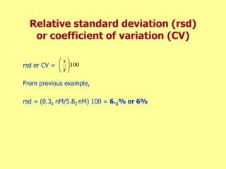
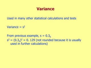
Basic of statistics
Mohammed suhaib
Statistics for Quantitative Analysis
• Statistics: Set of mathematical tools used to describe
and make judgments about data
• Type of statistics we will talk about in this class has
important assumption associated with it:
Experimental variation in the population from which samples
are drawn has a normal (Gaussian, bell-shaped) distribution.
- Parametric vs. non-parametric statistics
Normal distribution
• Infinite members of group:
population
• Characterize population by taking
samples
• The larger the number of samples,
the closer the distribution becomes to
normal
• Equation of normal distribution:
2
2
2
/
)
(
2
1 





 x
e
y
Normal distribution
• Estimate of mean value
of population = 
• Estimate of mean value
of samples =
Mean =
x
n
x
x i
i


Normal distribution
• Degree of scatter (measure of
central tendency) of population is
quantified by calculating the
standard deviation
• Std. dev. of population = 
• Std. dev. of sample = s
• Characterize sample by calculating
1
)
( 2




n
x
x
s
i
i
s
x 
Standard deviation and the
normal distribution
• Standard deviation
defines the shape of the
normal distribution
(particularly width)
• Larger std. dev. means
more scatter about the
mean, worse precision.
• Smaller std. dev. means
less scatter about the
mean, better precision.
Standard deviation and the
normal distribution
• There is a well-defined relationship
between the std. dev. of a population
and the normal distribution of the
population:
•  ± 1 encompasses 68.3 % of
measurements
•  ± 2 encompasses 95.5% of
measurements
•  ± 3 encompasses 99.7% of
measurements
• (May also consider these percentages
of area under the curve)
Example of mean and standard
deviation calculation
Consider Cu data: 5.23, 5.79, 6.21, 5.88, 6.02 nM
= 5.826 nM  5.82 nM
s = 0.368 nM  0.36 nM
Answer: 5.82 ± 0.36 nM or 5.8 ± 0.4 nM
Learn how to use the statistical functions on your
calculator. Do this example by longhand calculation
once, and also by calculator to verify that you’ll get
exactly the same answer. Then use your calculator for
all future calculations.
x
Relative standard deviation (rsd)
or coefficient of variation (CV)
rsd or CV =
From previous example,
rsd = (0.36 nM/5.82 nM) 100 = 6.1% or 6%
100






x
s
Standard error
• Tells us that standard deviation of set of samples should
decrease if we take more measurements
• Standard error =
• Take twice as many measurements, s decreases by
• Take 4x as many measurements, s decreases by
• There are several quantitative ways to determine the sample
size required to achieve a desired precision for various statistical
applications. Can consult statistics textbooks for further
information; e.g. J.H. Zar, Biostatistical Analysis
n
s
sx 
4
.
1
2 
2
4 
Variance
Used in many other statistical calculations and tests
Variance = s2
From previous example, s = 0.36
s2 = (0.36)2 = 0. 129 (not rounded because it is usually
used in further calculations)
Average deviation
• Another way to express
degree of scatter or
uncertainty in data. Not as
statistically meaningful as
standard deviation, but
useful for small samples.
Using previous data:
n
x
x
d i
i
 

)
(
5
8
.
5
02
.
6
8
.
5
88
.
5
8
.
5
21
.
6
8
.
5
79
.
5
8
.
5
23
.
5 2
2
2
2
2 









d
nM
or
d 2
.
0
2
.
0
25
.
0 5


nM
or
nM
Answer 2
.
0
8
.
5
2
.
0
8
.
5
: 5
2 

Relative average deviation (RAD)
Using previous data,
RAD = (0. 25/5.82) 100 = 4.2 or 4%
RAD = (0. 25/5.82) 1000 = 42 ppt
 4.2 x 101 or 4 x 101 ppt (0/00)
)
,
(
1000
)
(
100
ppt
thousand
per
parts
as
x
d
RAD
percentage
as
x
d
RAD


















Some useful statistical tests
• To characterize or make judgments about data
• Tests that use the Student’s t distribution
– Confidence intervals
– Comparing a measured result with a “known”
value
– Comparing replicate measurements (comparison
of means of two sets of data)

presentation_statistics_1448025870_153985.ppt

  • 1.
  • 2.
    Statistics for QuantitativeAnalysis • Statistics: Set of mathematical tools used to describe and make judgments about data • Type of statistics we will talk about in this class has important assumption associated with it: Experimental variation in the population from which samples are drawn has a normal (Gaussian, bell-shaped) distribution. - Parametric vs. non-parametric statistics
  • 3.
    Normal distribution • Infinitemembers of group: population • Characterize population by taking samples • The larger the number of samples, the closer the distribution becomes to normal • Equation of normal distribution: 2 2 2 / ) ( 2 1        x e y
  • 4.
    Normal distribution • Estimateof mean value of population =  • Estimate of mean value of samples = Mean = x n x x i i  
  • 5.
    Normal distribution • Degreeof scatter (measure of central tendency) of population is quantified by calculating the standard deviation • Std. dev. of population =  • Std. dev. of sample = s • Characterize sample by calculating 1 ) ( 2     n x x s i i s x 
  • 6.
    Standard deviation andthe normal distribution • Standard deviation defines the shape of the normal distribution (particularly width) • Larger std. dev. means more scatter about the mean, worse precision. • Smaller std. dev. means less scatter about the mean, better precision.
  • 7.
    Standard deviation andthe normal distribution • There is a well-defined relationship between the std. dev. of a population and the normal distribution of the population: •  ± 1 encompasses 68.3 % of measurements •  ± 2 encompasses 95.5% of measurements •  ± 3 encompasses 99.7% of measurements • (May also consider these percentages of area under the curve)
  • 8.
    Example of meanand standard deviation calculation Consider Cu data: 5.23, 5.79, 6.21, 5.88, 6.02 nM = 5.826 nM  5.82 nM s = 0.368 nM  0.36 nM Answer: 5.82 ± 0.36 nM or 5.8 ± 0.4 nM Learn how to use the statistical functions on your calculator. Do this example by longhand calculation once, and also by calculator to verify that you’ll get exactly the same answer. Then use your calculator for all future calculations. x
  • 9.
    Relative standard deviation(rsd) or coefficient of variation (CV) rsd or CV = From previous example, rsd = (0.36 nM/5.82 nM) 100 = 6.1% or 6% 100       x s
  • 10.
    Standard error • Tellsus that standard deviation of set of samples should decrease if we take more measurements • Standard error = • Take twice as many measurements, s decreases by • Take 4x as many measurements, s decreases by • There are several quantitative ways to determine the sample size required to achieve a desired precision for various statistical applications. Can consult statistics textbooks for further information; e.g. J.H. Zar, Biostatistical Analysis n s sx  4 . 1 2  2 4 
  • 11.
    Variance Used in manyother statistical calculations and tests Variance = s2 From previous example, s = 0.36 s2 = (0.36)2 = 0. 129 (not rounded because it is usually used in further calculations)
  • 12.
    Average deviation • Anotherway to express degree of scatter or uncertainty in data. Not as statistically meaningful as standard deviation, but useful for small samples. Using previous data: n x x d i i    ) ( 5 8 . 5 02 . 6 8 . 5 88 . 5 8 . 5 21 . 6 8 . 5 79 . 5 8 . 5 23 . 5 2 2 2 2 2           d nM or d 2 . 0 2 . 0 25 . 0 5   nM or nM Answer 2 . 0 8 . 5 2 . 0 8 . 5 : 5 2  
  • 13.
    Relative average deviation(RAD) Using previous data, RAD = (0. 25/5.82) 100 = 4.2 or 4% RAD = (0. 25/5.82) 1000 = 42 ppt  4.2 x 101 or 4 x 101 ppt (0/00) ) , ( 1000 ) ( 100 ppt thousand per parts as x d RAD percentage as x d RAD                  
  • 14.
    Some useful statisticaltests • To characterize or make judgments about data • Tests that use the Student’s t distribution – Confidence intervals – Comparing a measured result with a “known” value – Comparing replicate measurements (comparison of means of two sets of data)