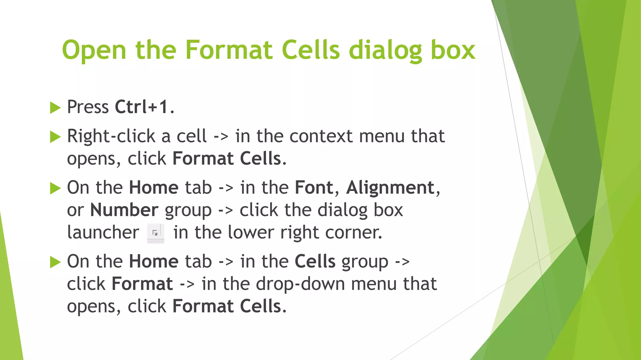
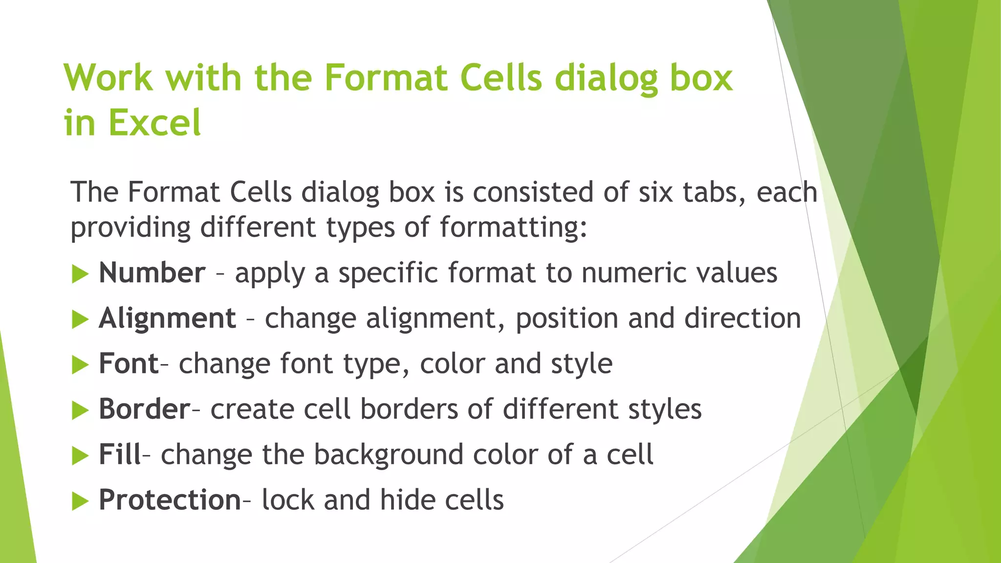
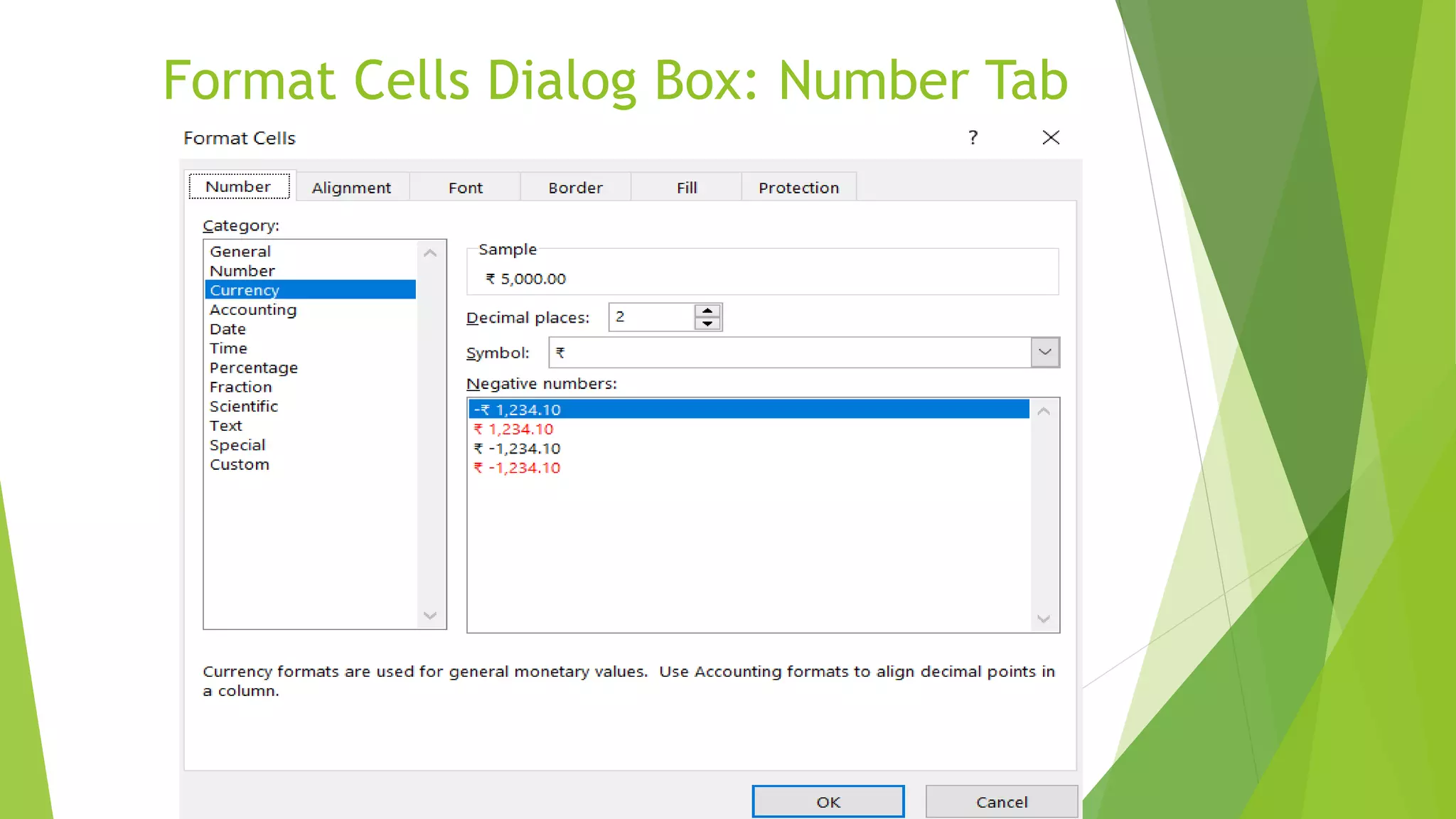
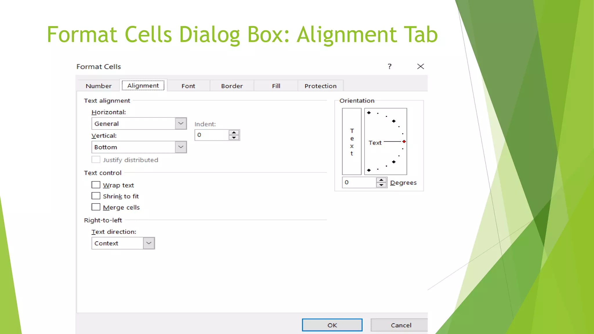
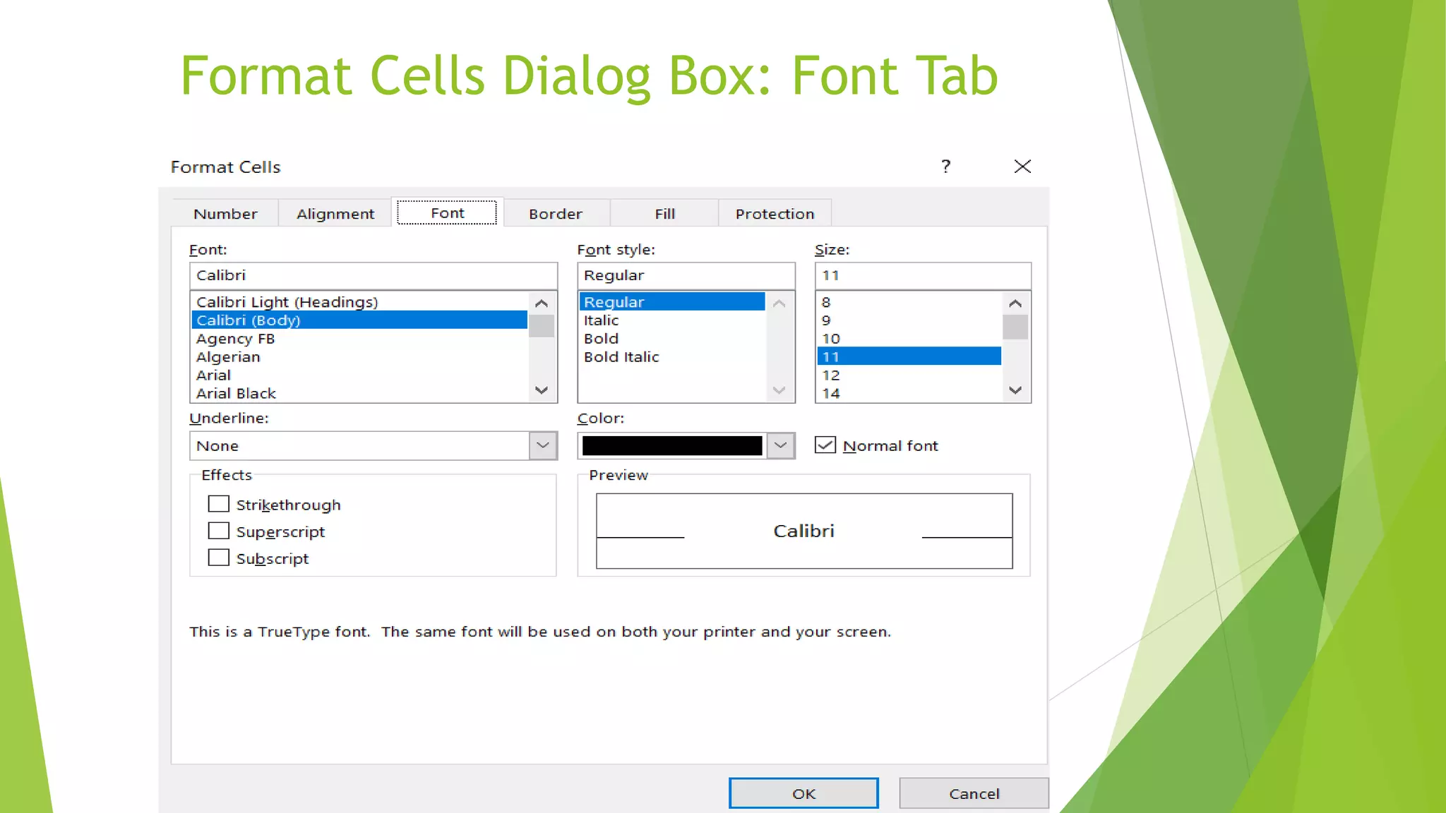
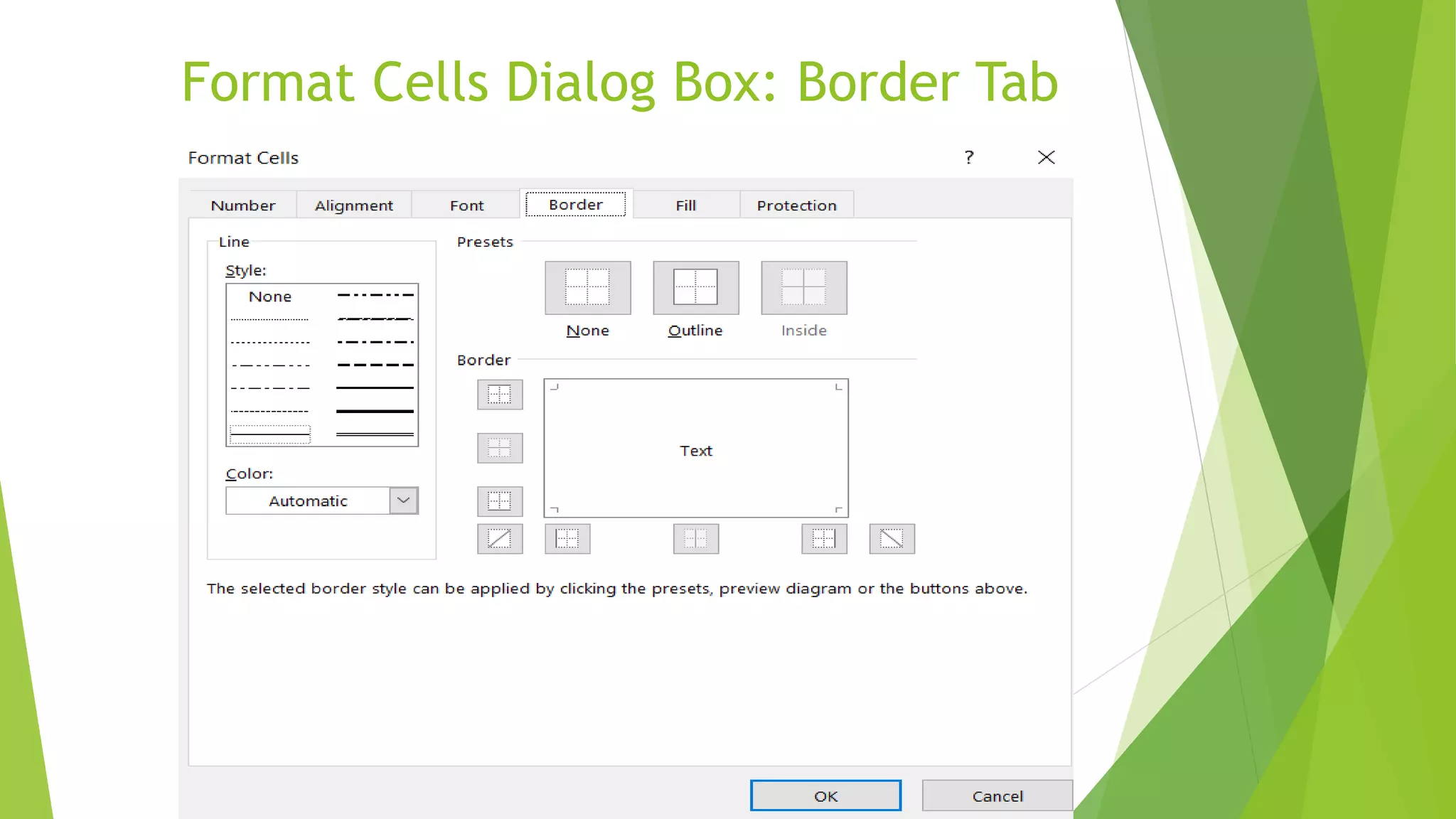
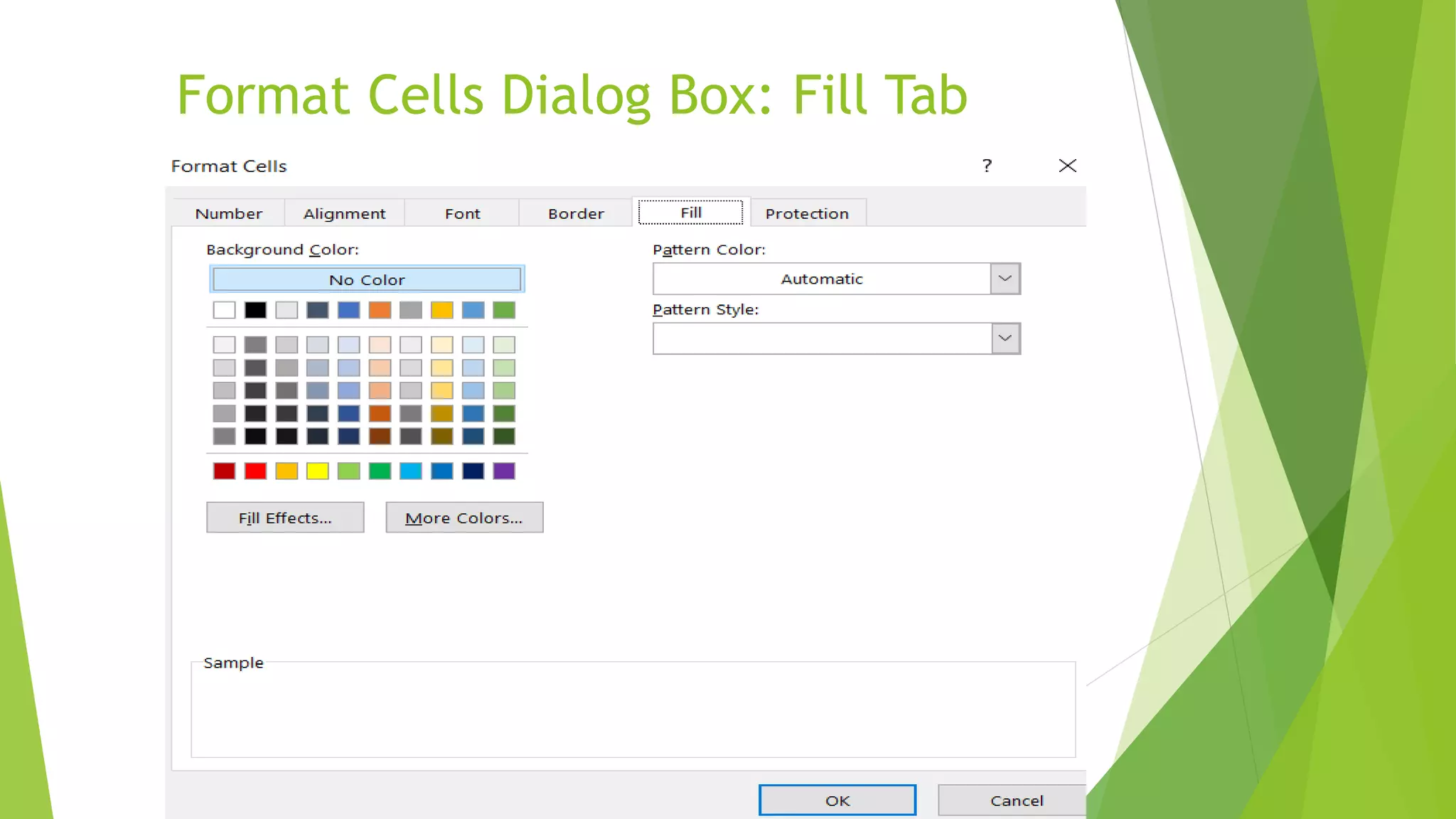
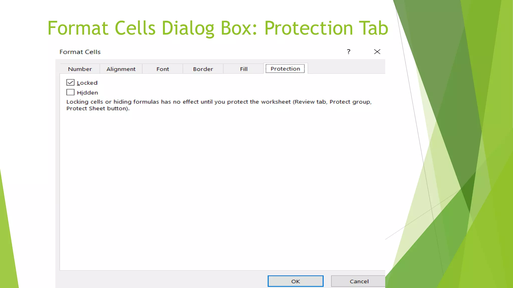
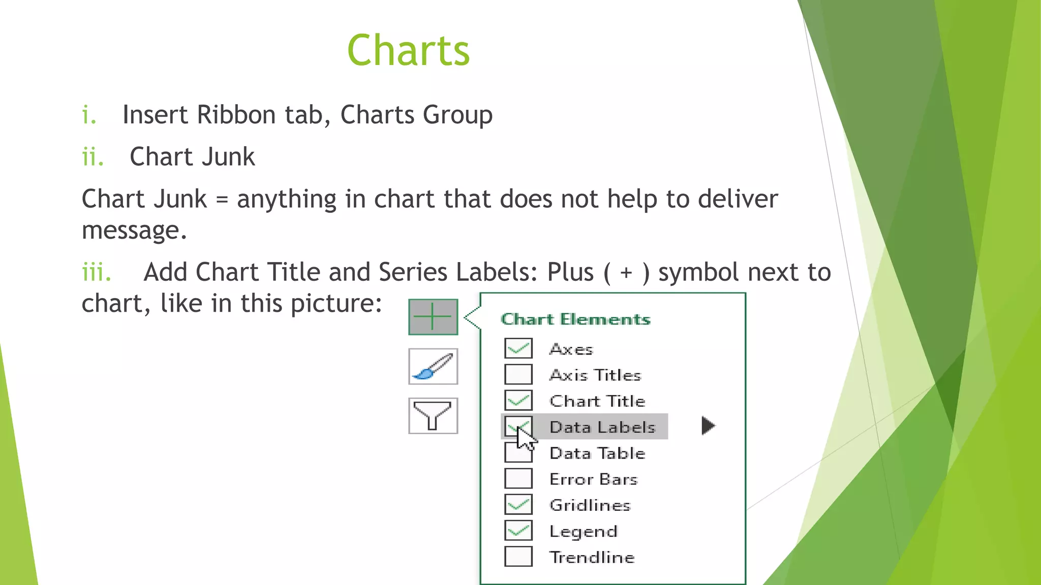
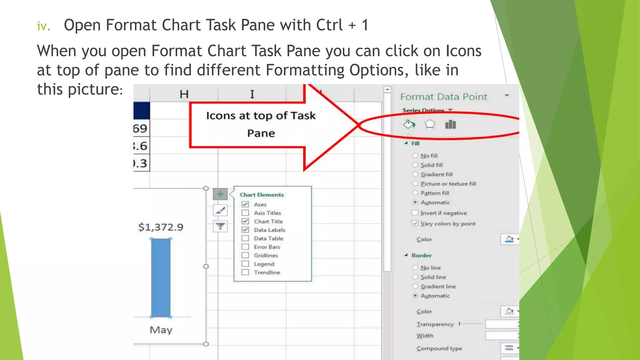
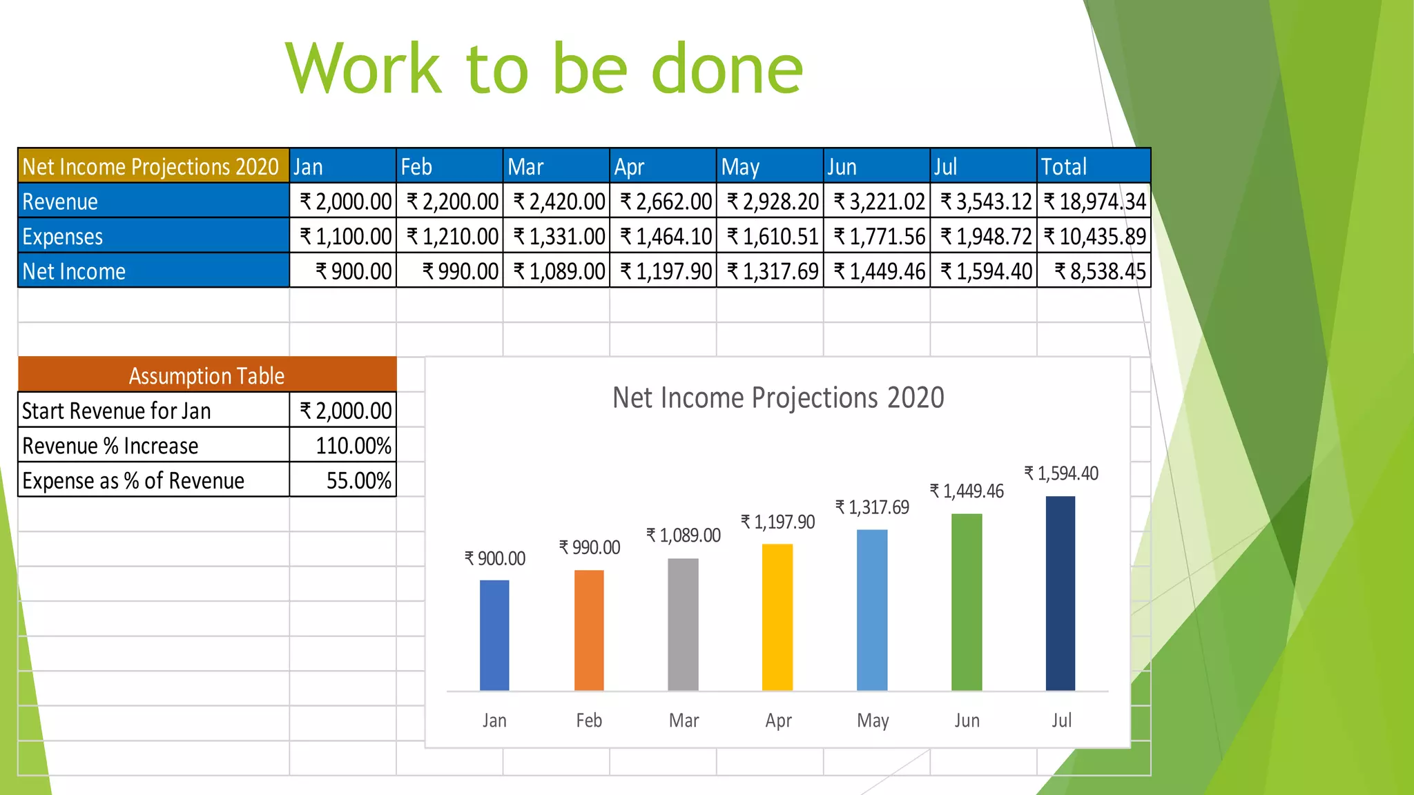
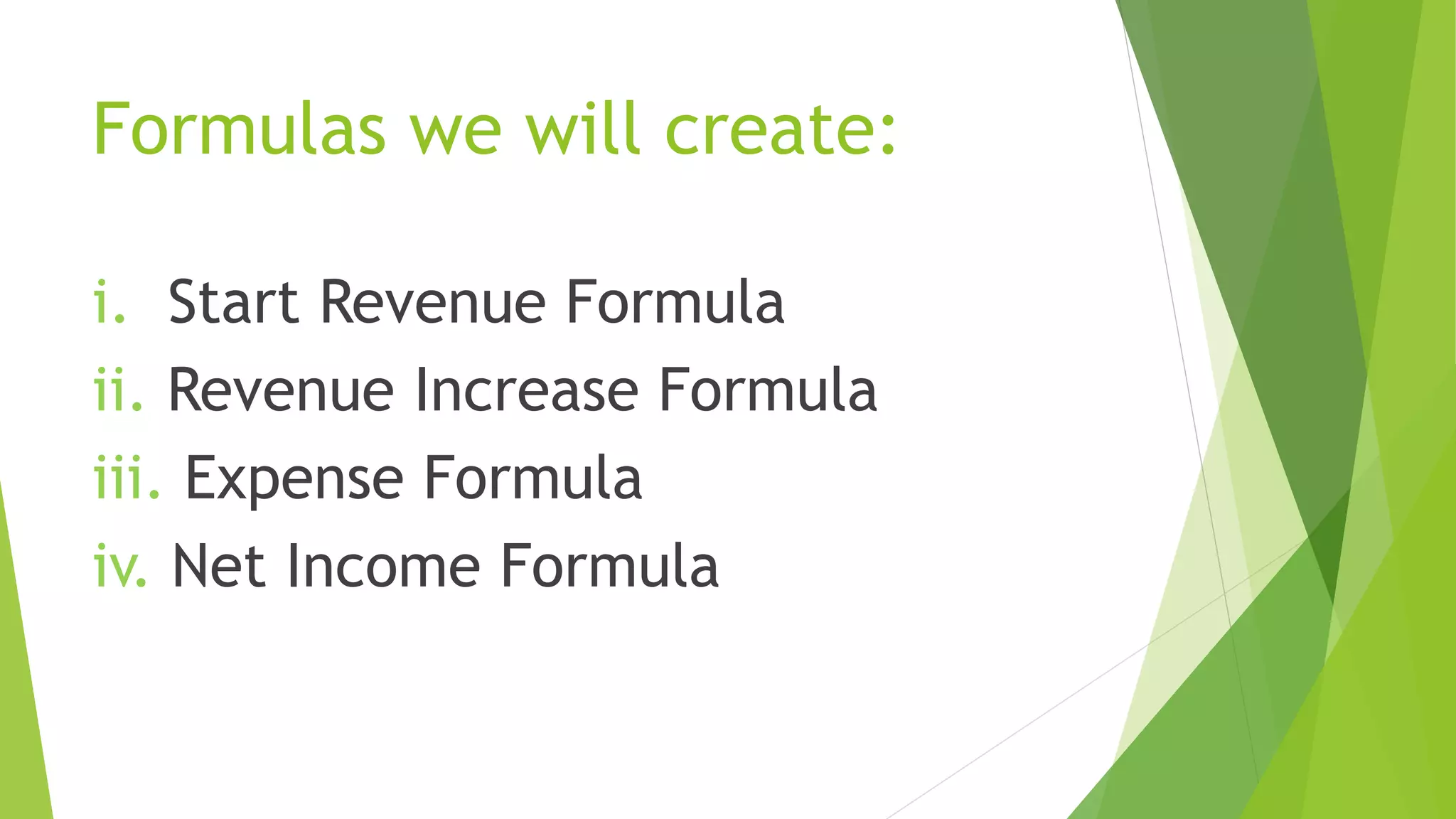
Presentation on MS Excel
Niyati Nangia
Topics to be covered:
Format Cells Dialog Box
Charts
Excel’s Golden Rule
Create Net Income Projections
Table
Open the Format Cells dialog box
 Press Ctrl+1.
 Right-click a cell -> in the context menu that
opens, click Format Cells.
 On the Home tab -> in the Font, Alignment,
or Number group -> click the dialog box
launcher in the lower right corner.
 On the Home tab -> in the Cells group ->
click Format -> in the drop-down menu that
opens, click Format Cells.
Work with the Format Cells dialog box
in Excel
The Format Cells dialog box is consisted of six tabs, each
providing different types of formatting:
 Number – apply a specific format to numeric values
 Alignment – change alignment, position and direction
 Font– change font type, color and style
 Border– create cell borders of different styles
 Fill– change the background color of a cell
 Protection– lock and hide cells
Format Cells Dialog Box: Number Tab
Format Cells Dialog Box: Alignment Tab
Format Cells Dialog Box: Font Tab
Format Cells Dialog Box: Border Tab
Format Cells Dialog Box: Fill Tab
Format Cells Dialog Box: Protection Tab
Charts
i. Insert Ribbon tab, Charts Group
ii. Chart Junk
Chart Junk = anything in chart that does not help to deliver
message.
iii. Add Chart Title and Series Labels: Plus ( + ) symbol next to
chart, like in this picture:
iv. Open Format Chart Task Pane with Ctrl + 1
When you open Format Chart Task Pane you can click on Icons
at top of pane to find different Formatting Options, like in
this picture:
 You can link the Chart Title to a cell:
1. Click on Chart Label and make sure it shows a
solid line (not a dashed line)
2. Click in Formula Bar
3. Type Equal sign
4. Click on cell in worksheet that has label
5. Hit Enter
Excel’s Golden Rule:
i. If a formula input can change, put it into a cell and
refer to it in the formula with a cell reference.
ii. If a formula input will not change, you can type it
into a formula (like 12 months in a year or 7 days in a
week).
iii. Always label your formula inputs so that the formula
input can be clearly understood by any user of the
spreadsheet solution; by doing this we properly
document the spreadsheet solution.
Work to be done
Net Income Projections 2020 Jan Feb Mar Apr May Jun Jul Total
Revenue ₹ 2,000.00 ₹ 2,200.00 ₹ 2,420.00 ₹ 2,662.00 ₹ 2,928.20 ₹ 3,221.02 ₹ 3,543.12 ₹ 18,974.34
Expenses ₹ 1,100.00 ₹ 1,210.00 ₹ 1,331.00 ₹ 1,464.10 ₹ 1,610.51 ₹ 1,771.56 ₹ 1,948.72 ₹ 10,435.89
Net Income ₹ 900.00 ₹ 990.00 ₹ 1,089.00 ₹ 1,197.90 ₹ 1,317.69 ₹ 1,449.46 ₹ 1,594.40 ₹ 8,538.45
Start Revenue for Jan ₹ 2,000.00
Revenue % Increase 110.00%
Expense as % of Revenue 55.00%
Assumption Table
₹ 900.00
₹ 990.00
₹ 1,089.00
₹ 1,197.90
₹ 1,317.69
₹ 1,449.46
₹ 1,594.40
Jan Feb Mar Apr May Jun Jul
Net Income Projections 2020
Formulas we will create:
i. Start Revenue Formula
ii. Revenue Increase Formula
iii. Expense Formula
iv. Net Income Formula

Presentation on MS Excel-4.pptx

  • 1.
    Presentation on MSExcel Niyati Nangia
  • 2.
    Topics to becovered: Format Cells Dialog Box Charts Excel’s Golden Rule Create Net Income Projections Table
  • 3.
    Open the FormatCells dialog box  Press Ctrl+1.  Right-click a cell -> in the context menu that opens, click Format Cells.  On the Home tab -> in the Font, Alignment, or Number group -> click the dialog box launcher in the lower right corner.  On the Home tab -> in the Cells group -> click Format -> in the drop-down menu that opens, click Format Cells.
  • 4.
    Work with theFormat Cells dialog box in Excel The Format Cells dialog box is consisted of six tabs, each providing different types of formatting:  Number – apply a specific format to numeric values  Alignment – change alignment, position and direction  Font– change font type, color and style  Border– create cell borders of different styles  Fill– change the background color of a cell  Protection– lock and hide cells
  • 5.
    Format Cells DialogBox: Number Tab
  • 6.
    Format Cells DialogBox: Alignment Tab
  • 7.
    Format Cells DialogBox: Font Tab
  • 8.
    Format Cells DialogBox: Border Tab
  • 9.
    Format Cells DialogBox: Fill Tab
  • 10.
    Format Cells DialogBox: Protection Tab
  • 11.
    Charts i. Insert Ribbontab, Charts Group ii. Chart Junk Chart Junk = anything in chart that does not help to deliver message. iii. Add Chart Title and Series Labels: Plus ( + ) symbol next to chart, like in this picture:
  • 12.
    iv. Open FormatChart Task Pane with Ctrl + 1 When you open Format Chart Task Pane you can click on Icons at top of pane to find different Formatting Options, like in this picture:
  • 13.
     You canlink the Chart Title to a cell: 1. Click on Chart Label and make sure it shows a solid line (not a dashed line) 2. Click in Formula Bar 3. Type Equal sign 4. Click on cell in worksheet that has label 5. Hit Enter
  • 14.
    Excel’s Golden Rule: i.If a formula input can change, put it into a cell and refer to it in the formula with a cell reference. ii. If a formula input will not change, you can type it into a formula (like 12 months in a year or 7 days in a week). iii. Always label your formula inputs so that the formula input can be clearly understood by any user of the spreadsheet solution; by doing this we properly document the spreadsheet solution.
  • 15.
    Work to bedone Net Income Projections 2020 Jan Feb Mar Apr May Jun Jul Total Revenue ₹ 2,000.00 ₹ 2,200.00 ₹ 2,420.00 ₹ 2,662.00 ₹ 2,928.20 ₹ 3,221.02 ₹ 3,543.12 ₹ 18,974.34 Expenses ₹ 1,100.00 ₹ 1,210.00 ₹ 1,331.00 ₹ 1,464.10 ₹ 1,610.51 ₹ 1,771.56 ₹ 1,948.72 ₹ 10,435.89 Net Income ₹ 900.00 ₹ 990.00 ₹ 1,089.00 ₹ 1,197.90 ₹ 1,317.69 ₹ 1,449.46 ₹ 1,594.40 ₹ 8,538.45 Start Revenue for Jan ₹ 2,000.00 Revenue % Increase 110.00% Expense as % of Revenue 55.00% Assumption Table ₹ 900.00 ₹ 990.00 ₹ 1,089.00 ₹ 1,197.90 ₹ 1,317.69 ₹ 1,449.46 ₹ 1,594.40 Jan Feb Mar Apr May Jun Jul Net Income Projections 2020
  • 16.
    Formulas we willcreate: i. Start Revenue Formula ii. Revenue Increase Formula iii. Expense Formula iv. Net Income Formula