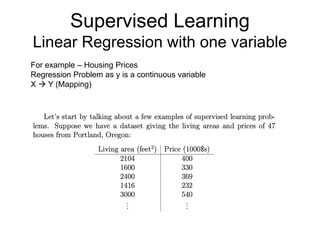
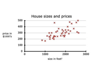
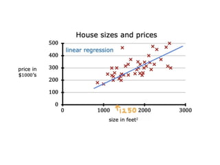
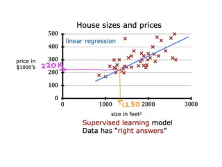
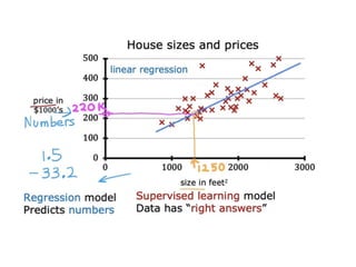
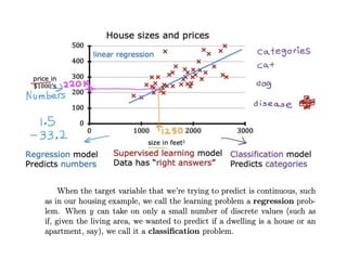
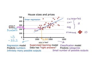
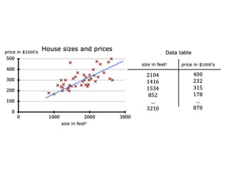
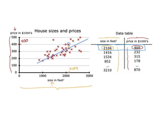
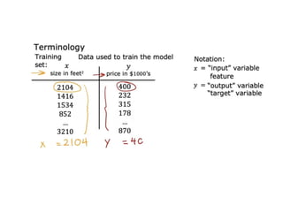
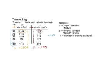
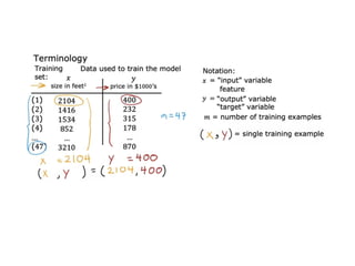
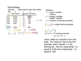
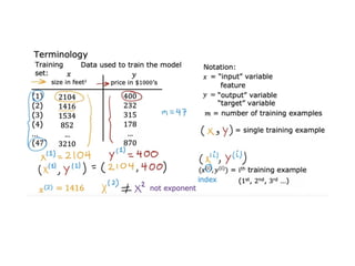
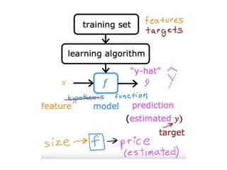
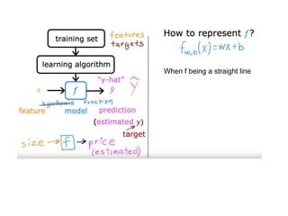
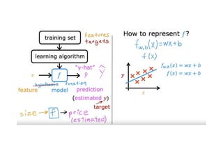
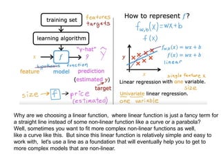
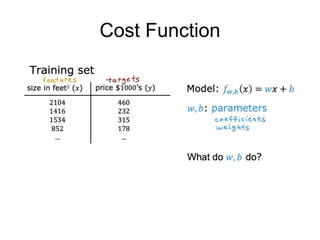
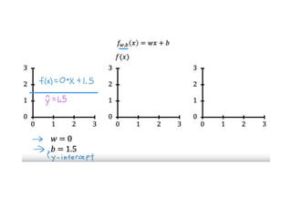
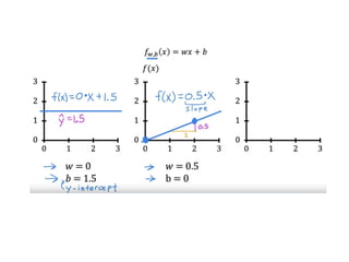
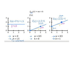
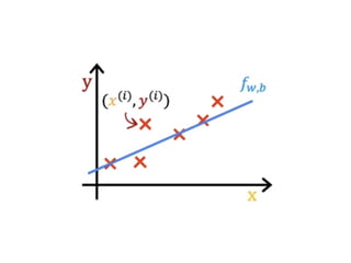
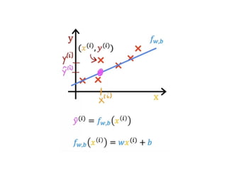
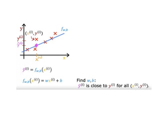
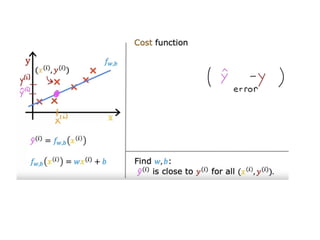
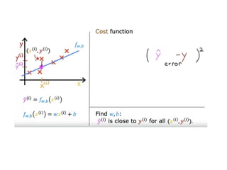
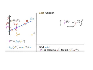
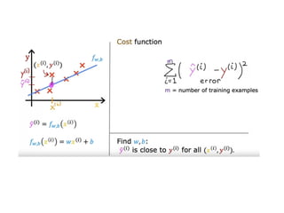
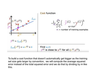
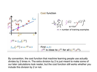
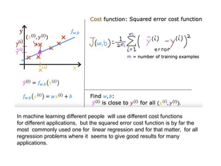
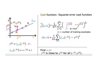
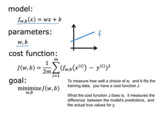
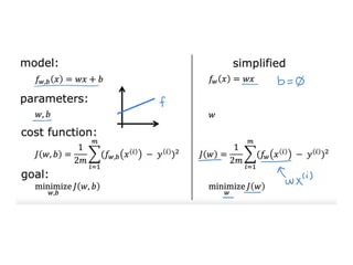
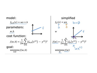
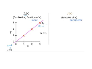
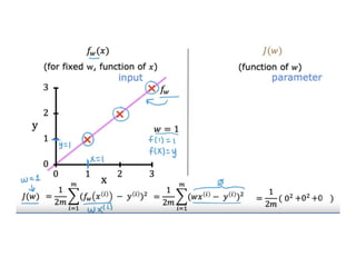
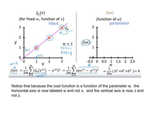
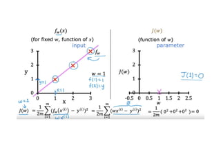
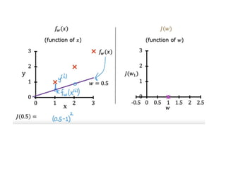
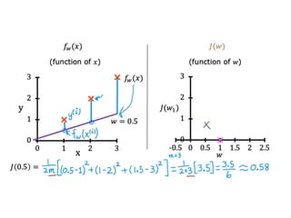
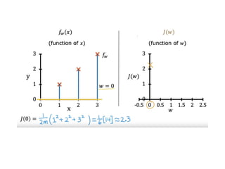
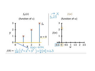
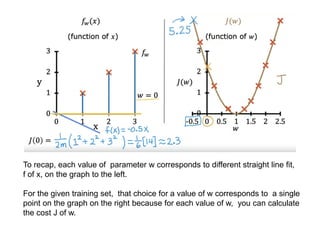
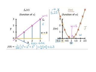
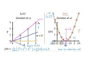
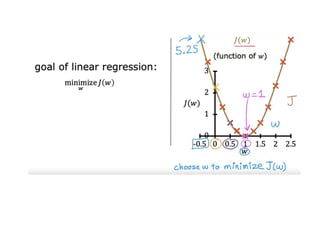
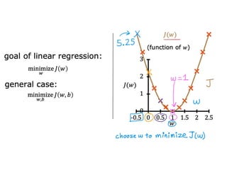
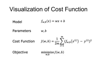
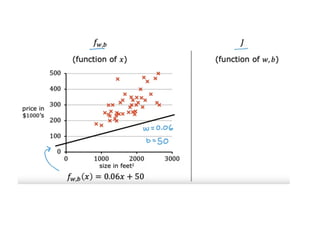
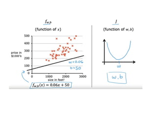
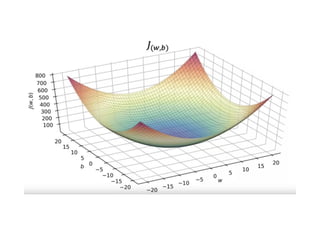
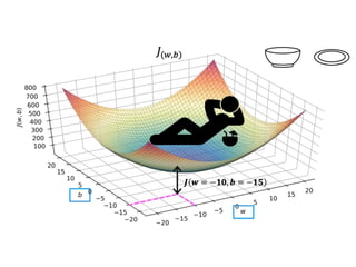
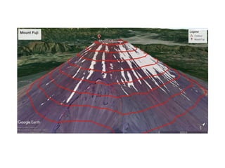
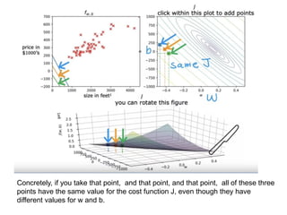
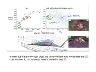
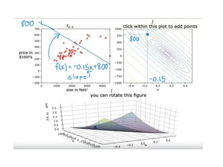
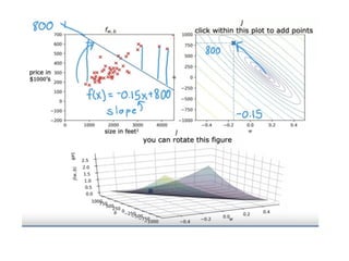
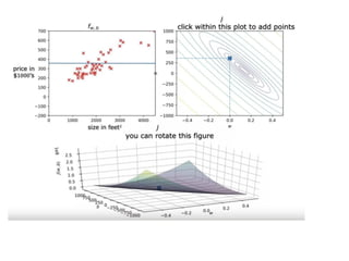
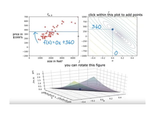
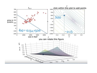
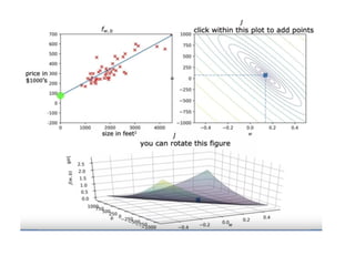
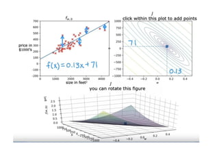
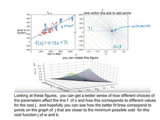
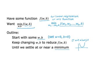
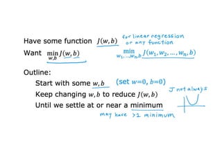
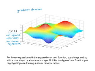
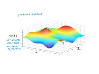
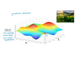
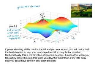
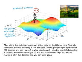
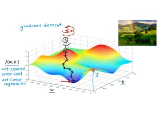
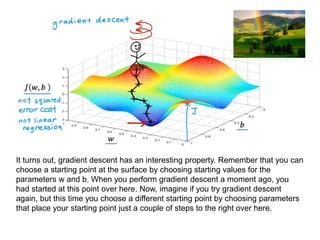
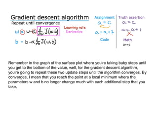
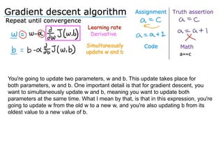
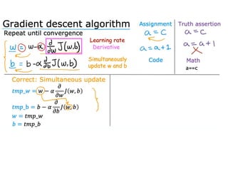
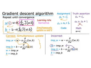
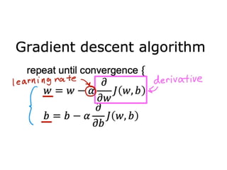
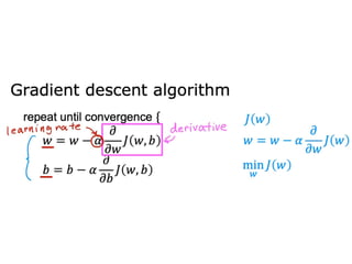
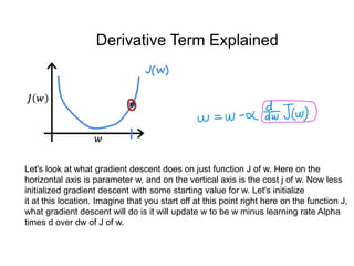
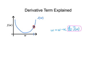
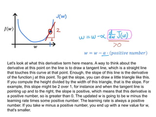
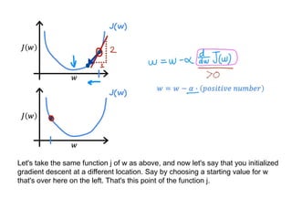
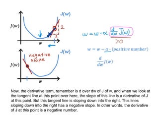
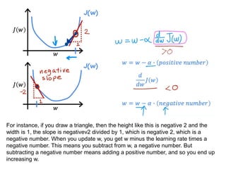
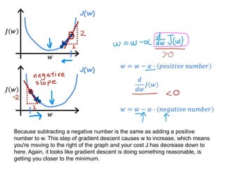
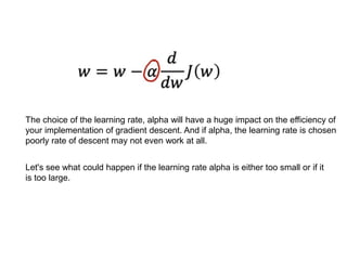
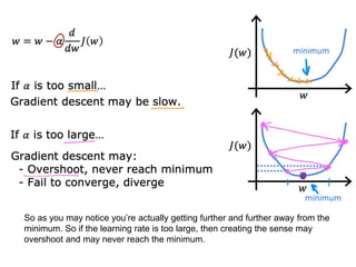
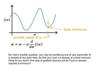
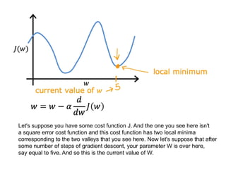
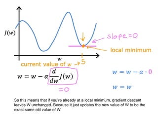
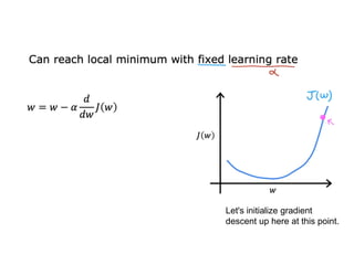
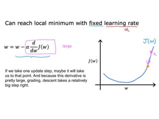
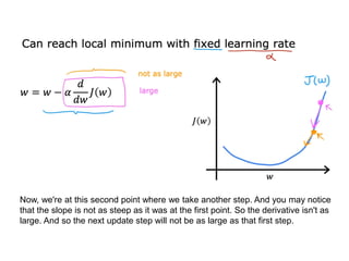
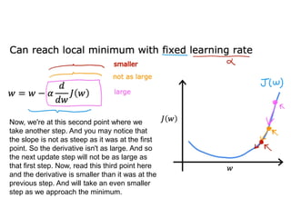
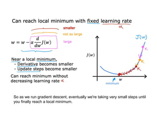
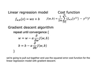
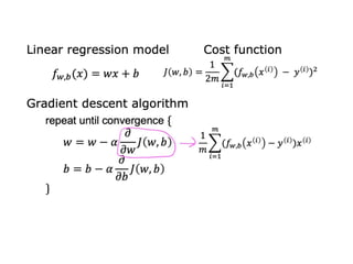
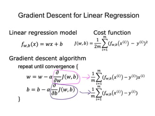
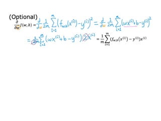
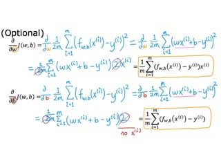
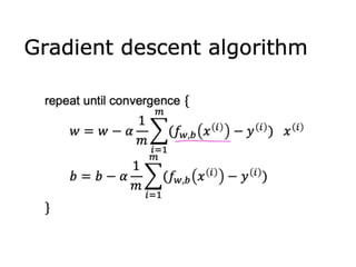
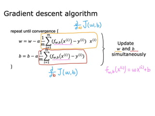
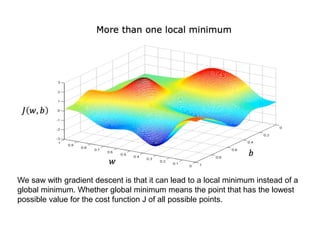
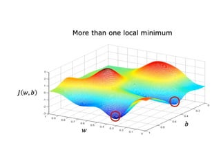
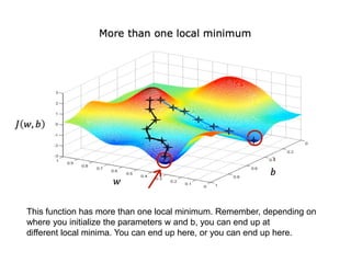
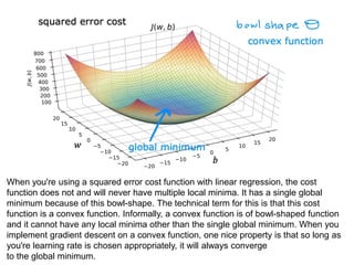
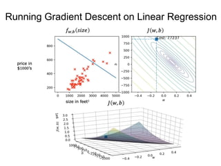
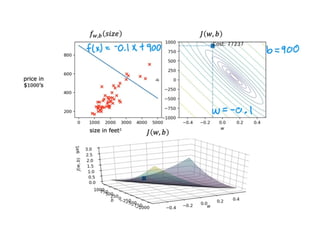
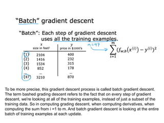
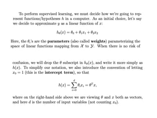
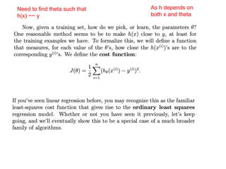
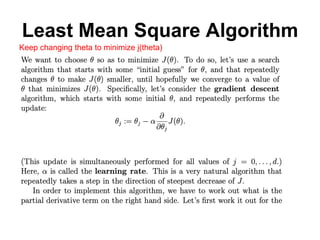
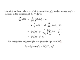
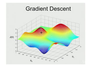
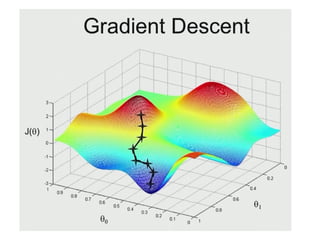
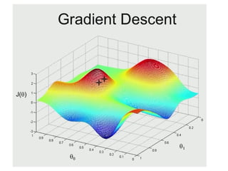
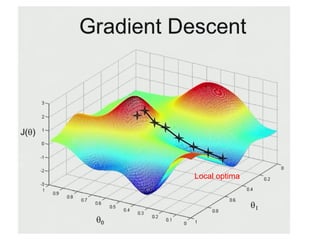
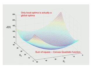
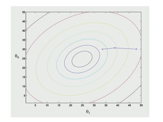
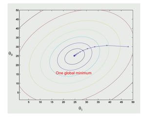
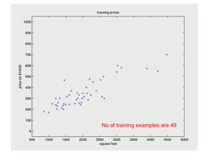
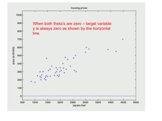
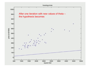
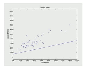
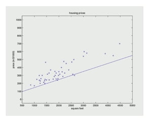
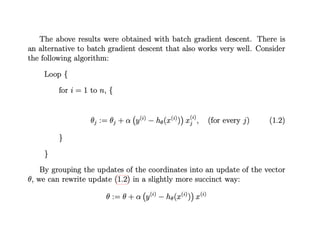
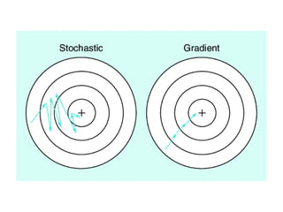
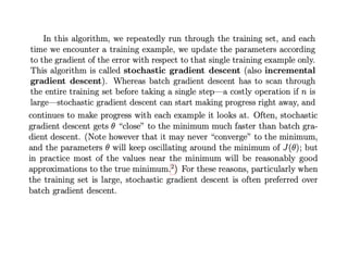
SlideShare a Scribd company logo
1 of 171
Download to read offline
Supervised Learning
Linear Regression with one variable
For example – Housing Prices
Regression Problem as y is a continuous variable
X → Y (Mapping)
i here, refers to a specific row in the
table. For instance, here is the first
example, when i equals 1 in the
training set, and so x superscript 1 is
equal to 2104 and y superscript 1 is
equal to 400
When f being a straight line
Why are we choosing a linear function, where linear function is just a fancy term for
a straight line instead of some non-linear function like a curve or a parabola?
Well, sometimes you want to fit more complex non-linear functions as well,
like a curve like this. But since this linear function is relatively simple and easy to
work with, let's use a line as a foundation that will eventually help you to get to
more complex models that are non-linear.
Cost Function
To build a cost function that doesn't automatically get bigger as the training
set size gets larger by convention, we will compute the average squared
error instead of the total squared error and we do that by dividing by m like
this.
By convention, the cost function that machine learning people use actually
divides by 2 times m. The extra division by 2 is just meant to make some of
our later calculations look neater, but the cost function still works whether you
include this division by 2 or not.
In machine learning different people will use different cost functions
for different applications, but the squared error cost function is by far the
most commonly used one for linear regression and for that matter, for all
regression problems where it seems to give good results for many
applications.
To measure how well a choice of w, and b fits the
training data, you have a cost function J.
What the cost function J does is, it measures the
difference between the model's predictions, and
the actual true values for y.
Notice that because the cost function is a function of the parameter w, the
horizontal axis is now labeled w and not x, and the vertical axis is now J and
not y.
To recap, each value of parameter w corresponds to different straight line fit,
f of x, on the graph to the left.
For the given training set, that choice for a value of w corresponds to a single
point on the graph on the right because for each value of w, you can calculate
the cost J of w.
Visualization of Cost Function
Concretely, if you take that point, and that point, and that point, all of these three
points have the same value for the cost function J, even though they have
different values for w and b.
It turns out that the contour plots are a convenient way to visualize the 3D
cost function J, but in a way, there's plotted in just 2D.
Looking at these figures, you can get a better sense of how different choices of
the parameters affect the line f of x and how this corresponds to different values
for the cost j, and hopefully you can see how the better fit lines correspond to
points on the graph of j that are closer to the minimum possible cost for this
cost function j of w and b.
We can write in code for automatically finding the
values of parameters w and b they give you the best-
fit line. That minimizes the
cost function j.
There is an algorithm for doing this called gradient
descent. This algorithm is one of the most important
algorithms in machine learning.
Gradient descent and variations on gradient descent
are used to train not just linear regression but some
of the biggest and most complex models in all of AI.
Gradient Descent Algorithm
Gradient descent will set you up with one of the most
important building blocks in machine learning.
Gradient descent is an algorithm that you can use to
try to minimize any function.
Gradient Descent Algorithm
For linear regression with the squared error cost function, you always end up
with a bow shape or a hammock shape. But this is a type of cost function you
might get if you're training a neural network model.
if you're standing at this point in the hill and you look around, you will notice that
the best direction to take your next step downhill is roughly that direction.
Mathematically, this is the direction of steepest descent. It means that when you
take a tiny baby little step, this takes you downhill faster than a tiny little baby
step you could have taken in any other direction.
After taking this first step, you're now at this point on the hill over here. Now let's
repeat the process. Standing at this new point, you're going to again spin around
360 degrees and ask yourself, in what direction will I take the next little baby step
in order to move downhill? If you do that and take another step, you end up
moving a bit in that direction and you can keep going.
It turns out, gradient descent has an interesting property. Remember that you can
choose a starting point at the surface by choosing starting values for the
parameters w and b. When you perform gradient descent a moment ago, you
had started at this point over here. Now, imagine if you try gradient descent
again, but this time you choose a different starting point by choosing parameters
that place your starting point just a couple of steps to the right over here.
If you then repeat the gradient descent process, which means you look around,
take a little step in the direction of steepest ascent so you end up here. Then you
again look around, take another step, and so on. If you were to run gradient
descent this second time, starting just a couple steps in the right of where we did it
the first time, then you end up in a totally different valley. This different minimum
over here on the right.
The bottoms of both the first and the second valleys are
called local minima. Because if you start going down the first valley, gradient
descent won't lead you to the second valley, and the same is true if you started
going down the second valley, you stay in that second minimum and not find your
way into the first local minimum. This is an interesting property of the gradient
descent algorithm
In this equation, Alpha is also called the learning rate. The learning rate is usually
a small positive number between 0 and 1 and it might be say, 0.01. What Alpha
does is, it basically controls how big of a step you take downhill. If Alpha is very
large, then that corresponds to a very aggressive gradient descent procedure
where you're trying to take huge steps downhill. If Alpha is very small, then you'd
be taking small baby steps downhill.
Remember in the graph of the surface plot where you're taking baby steps until
you get to the bottom of the value, well, for the gradient descent algorithm,
you're going to repeat these two update steps until the algorithm converges. By
converges, I mean that you reach the point at a local minimum where the
parameters w and b no longer change much with each additional step that you
take.
You're going to update two parameters, w and b. This update takes place for
both parameters, w and b. One important detail is that for gradient descent, you
want to simultaneously update w and b, meaning you want to update both
parameters at the same time. What I mean by that, is that in this expression, you're
going to update w from the old w to a new w, and you're also updating b from its
oldest value to a new value of b.
Derivative Term Explained
Let's look at what gradient descent does on just function J of w. Here on the
horizontal axis is parameter w, and on the vertical axis is the cost j of w. Now less
initialized gradient descent with some starting value for w. Let's initialize
it at this location. Imagine that you start off at this point right here on the function J,
what gradient descent will do is it will update w to be w minus learning rate Alpha
times d over dw of J of w.
Derivative Term Explained
Let's look at what this derivative term here means. A way to think about the
derivative at this point on the line is to draw a tangent line, which is a straight line
that touches this curve at that point. Enough, the slope of this line is the derivative
of the function j at this point. To get the slope, you can draw a little triangle like this.
If you compute the height divided by the width of this triangle, that is the slope. For
example, this slope might be 2 over 1, for instance and when the tangent line is
pointing up and to the right, the slope is positive, which means that this derivative is
a positive number, so is greater than 0. The updated w is going to be w minus the
learning rate times some positive number. The learning rate is always a positive
number. If you take w minus a positive number, you end up with a new value for w,
that's smaller.
On the graph, you’re moving to the left, you're decreasing the value of w. You
may notice that this is the right thing to do if your goal is to decrease the cost J,
because when we move towards the left on this curve, the cost j decreases, and
you're getting closer to the minimum for J, which is over here. So far, gradient
descent, seems to be doing the right thing.
Let's take the same function j of w as above, and now let's say that you initialized
gradient descent at a different location. Say by choosing a starting value for w
that's over here on the left. That's this point of the function j.
Now, the derivative term, remember is d over dw of J of w, and when we look at
the tangent line at this point over here, the slope of this line is a derivative of J
at this point. But this tangent line is sloping down into the right. This lines
sloping down into the right has a negative slope. In other words, the derivative
of J at this point is a negative number.
For instance, if you draw a triangle, then the height like this is negative 2 and the
width is 1, the slope is negativev2 divided by 1, which is negative 2, which is a
negative number. When you update w, you get w minus the learning rate times a
negative number. This means you subtract from w, a negative number. But
subtracting a negative number means adding a positive number, and so you end up
increasing w.
Because subtracting a negative number is the same as adding a positive
number to w. This step of gradient descent causes w to increase, which means
you're moving to the right of the graph and your cost J has decrease down to
here. Again, it looks like gradient descent is doing something reasonable, is
getting you closer to the minimum.
The choice of the learning rate, alpha will have a huge impact on the efficiency of
your implementation of gradient descent. And if alpha, the learning rate is chosen
poorly rate of descent may not even work at all.
Let's see what could happen if the learning rate alpha is either too small or if it
is too large.
For the case where the learning rate is too small. Here's a graph where the horizontal
axis is W and the vertical axis is the cost J. And here's the graph of the function J of
W. Let's start grading descent at this point here, if the learning rate is too small. Then
what happens is that you multiply your derivative term by some really, really small
number. So you're going to be multiplying by number alpha. That's really small, like
0.0000001. And so you end up taking a very small baby step like that.
To summarize if the learning rate is too small, then gradient descents will work,
but it will be slow. It will take a very long time because it’s going to take these tiny
tiny baby steps. And it's going to need a lot of steps before it gets anywhere close to
the minimum.
What happens if the learning rate is too large? Here's another graph of the cost
function. And let's say we start grating descent with W at this value here. So it's
actually already pretty close to the minimum.
But if the learning rate is too large then you update W very giant step to be all the
way over here. And that's this point here on the function J. So you move from this
point on the left, all the way to this point on the right. And now the cost has
actually gotten worse. It has increased because it started out at this value here
and after one step, it actually increased to this value here.
Now the derivative at this new point says to decrease W but when the learning rate
is too big. Then you may take a huge step going from here all the way out here. So
now you've gotten to this point here and again, if the learning rate is too big. Then
you take another huge step with an acceleration and way overshoot the minimum
again.
So as you may notice you’re actually getting further and further away from the
minimum. So if the learning rate is too large, then creating the sense may
overshoot and may never reach the minimum.
So, here's another question, you may be wondering one of your parameter W
is already at this point here. So that your cost J is already at a local minimum.
What do you think? One step of gradient descent will do if you've already
reached a minimum?
Let's suppose you have some cost function J. And the one you see here isn't
a square error cost function and this cost function has two local minima
corresponding to the two valleys that you see here. Now let's suppose that after
some number of steps of gradient descent, your parameter W is over here,
say equal to five. And so this is the current value of W.
So this means that if you’re already at a local minimum, gradient descent
leaves W unchanged. Because it just updates the new value of W to be the
exact same old value of W.
Let's initialize gradient
descent up here at this point.
If we take one update step, maybe it will take
us to that point. And because this derivative is
pretty large, grading, descent takes a relatively
big step right.
Now, we're at this second point where we take another step. And you may notice
that the slope is not as steep as it was at the first point. So the derivative isn't as
large. And so the next update step will not be as large as that first step.
Now, we're at this second point where we
take another step. And you may notice that
the slope is not as steep as it was at the first
point. So the derivative isn't as large. And so
the next update step will not be as large as
that first step. Now, read this third point here
and the derivative is smaller than it was at the
previous step. And will take an even smaller
step as we approach the minimum.
So as we run gradient descent, eventually we're taking very small steps until
you finally reach a local minimum.
we're going to pull out together and use the squared error cost function for the
linear regression model with gradient descent.
Gradient Descent for Linear Regression
We saw with gradient descent is that it can lead to a local minimum instead of a
global minimum. Whether global minimum means the point that has the lowest
possible value for the cost function J of all possible points.
This function has more than one local minimum. Remember, depending on
where you initialize the parameters w and b, you can end up at
different local minima. You can end up here, or you can end up here.
When you're using a squared error cost function with linear regression, the cost
function does not and will never have multiple local minima. It has a single global
minimum because of this bowl-shape. The technical term for this is that this cost
function is a convex function. Informally, a convex function is of bowl-shaped function
and it cannot have any local minima other than the single global minimum. When you
implement gradient descent on a convex function, one nice property is that so long as
you're learning rate is chosen appropriately, it will always converge
to the global minimum.
Running Gradient Descent on Linear Regression
For instance, if your friend’s house size is 1250 square feet, you can now read off the
value and predict that maybe they could get, $250,000 for the house.
To be more precise, this gradient descent process is called batch gradient descent.
The term bashed grading descent refers to the fact that on every step of gradient
descent, we're looking at all of the training examples, instead of just a subset of the
training data. So in computing grading descent, when computing derivatives, when
computing the sum from i =1 to m. And batch gradient descent is looking at the entire
batch of training examples at each update.
Optional Slides
Need to find theta such that
h(x) ~~ y
As h depends on
both x and theta
Least Mean Square Algorithm
Keep changing theta to minimize j(theta)
Linear Regression
Stochastic Gradient Descent
Stochastic gradient
descent is an
optimization algorithm
often used in machine
learning applications to
find the model
parameters that
correspond to the best
fit between predicted
and actual outputs.
Local optima
Only local optima is actually a
global optima
Sum of square – Convex Quadratic function
The ellipses shown above are the contours of a quadratic function. Also
shown is the trajectory taken by gradient descent, which was initialized at
(48,30). The x’s in the figure (joined by straight lines) mark the successive
values of θ that gradient descent went through.
One global minimum
No of training examples are 49
When both theta’s are zero – target variable
y is always zero as shown by the horizontal
line.
After one iteration with new values of theta –
the hypothesis becomes
Presentation about the Linear Regression.pdf

More Related Content

Similar to Presentation about the Linear Regression.pdf

Essay On Linear Function
Essay On Linear FunctionEssay On Linear Function
Essay On Linear Function
Angie Lee
 
Artifact 3 clemson
Artifact 3 clemsonArtifact 3 clemson
Artifact 3 clemson
clemsonj11
 
Slope and Equations of Lines
Slope and Equations of LinesSlope and Equations of Lines
Slope and Equations of Lines
powel2ra
 
Gauss jordan
Gauss jordanGauss jordan
Gauss jordan
uis
 
Antiderivatives And Slope Fields
Antiderivatives And Slope FieldsAntiderivatives And Slope Fields
Antiderivatives And Slope Fields
seltzermath
 
Inverse trig functions
Inverse trig functionsInverse trig functions
Inverse trig functions
Jessica Garcia
 

Similar to Presentation about the Linear Regression.pdf (20)

Essay On Linear Function
Essay On Linear FunctionEssay On Linear Function
Essay On Linear Function
 
Gradient Decent in Linear Regression.pptx
Gradient Decent in Linear Regression.pptxGradient Decent in Linear Regression.pptx
Gradient Decent in Linear Regression.pptx
 
Calculus I basic concepts
Calculus I basic conceptsCalculus I basic concepts
Calculus I basic concepts
 
Application of derivatives
Application of derivatives Application of derivatives
Application of derivatives
 
3D Math Primer: CocoaConf Chicago
3D Math Primer: CocoaConf Chicago3D Math Primer: CocoaConf Chicago
3D Math Primer: CocoaConf Chicago
 
Physics 1.3 scalars and vectors
Physics 1.3 scalars and vectorsPhysics 1.3 scalars and vectors
Physics 1.3 scalars and vectors
 
Artifact 3 clemson
Artifact 3 clemsonArtifact 3 clemson
Artifact 3 clemson
 
Slope and Equations of Lines
Slope and Equations of LinesSlope and Equations of Lines
Slope and Equations of Lines
 
Gauss jordan
Gauss jordanGauss jordan
Gauss jordan
 
Antiderivatives And Slope Fields
Antiderivatives And Slope FieldsAntiderivatives And Slope Fields
Antiderivatives And Slope Fields
 
Derivación e integración de funcione variables
Derivación e integración de funcione variablesDerivación e integración de funcione variables
Derivación e integración de funcione variables
 
Lec12
Lec12Lec12
Lec12
 
Lec12
Lec12Lec12
Lec12
 
Ann a Algorithms notes
Ann a Algorithms notesAnn a Algorithms notes
Ann a Algorithms notes
 
Detail Study of the concept of Regression model.pptx
Detail Study of the concept of  Regression model.pptxDetail Study of the concept of  Regression model.pptx
Detail Study of the concept of Regression model.pptx
 
Inverse trig functions
Inverse trig functionsInverse trig functions
Inverse trig functions
 
PRML Chapter 12
PRML Chapter 12PRML Chapter 12
PRML Chapter 12
 
Lecture 5 - Gradient Descent, a lecture in subject module Statistical & Machi...
Lecture 5 - Gradient Descent, a lecture in subject module Statistical & Machi...Lecture 5 - Gradient Descent, a lecture in subject module Statistical & Machi...
Lecture 5 - Gradient Descent, a lecture in subject module Statistical & Machi...
 
nonlinear programming
nonlinear programmingnonlinear programming
nonlinear programming
 
1.5 all notes
1.5 all notes1.5 all notes
1.5 all notes
 

Recently uploaded

一比一原版(Monash毕业证书)莫纳什大学毕业证成绩单如何办理
一比一原版(Monash毕业证书)莫纳什大学毕业证成绩单如何办理一比一原版(Monash毕业证书)莫纳什大学毕业证成绩单如何办理
一比一原版(Monash毕业证书)莫纳什大学毕业证成绩单如何办理
pyhepag
 
1:1原版定制伦敦政治经济学院毕业证(LSE毕业证)成绩单学位证书留信学历认证
1:1原版定制伦敦政治经济学院毕业证(LSE毕业证)成绩单学位证书留信学历认证1:1原版定制伦敦政治经济学院毕业证(LSE毕业证)成绩单学位证书留信学历认证
1:1原版定制伦敦政治经济学院毕业证(LSE毕业证)成绩单学位证书留信学历认证
dq9vz1isj
 
Audience Researchndfhcvnfgvgbhujhgfv.pptx
Audience Researchndfhcvnfgvgbhujhgfv.pptxAudience Researchndfhcvnfgvgbhujhgfv.pptx
Audience Researchndfhcvnfgvgbhujhgfv.pptx
Stephen266013
 
Toko Jual Viagra Asli Di Salatiga 081229400522 Obat Kuat Viagra
Toko Jual Viagra Asli Di Salatiga 081229400522 Obat Kuat ViagraToko Jual Viagra Asli Di Salatiga 081229400522 Obat Kuat Viagra
Toko Jual Viagra Asli Di Salatiga 081229400522 Obat Kuat Viagra
adet6151
 
如何办理哥伦比亚大学毕业证(Columbia毕业证)成绩单原版一比一
如何办理哥伦比亚大学毕业证(Columbia毕业证)成绩单原版一比一如何办理哥伦比亚大学毕业证(Columbia毕业证)成绩单原版一比一
如何办理哥伦比亚大学毕业证(Columbia毕业证)成绩单原版一比一
fztigerwe
 
Exploratory Data Analysis - Dilip S.pptx
Exploratory Data Analysis - Dilip S.pptxExploratory Data Analysis - Dilip S.pptx
Exploratory Data Analysis - Dilip S.pptx
DilipVasan
 
edited gordis ebook sixth edition david d.pdf
edited gordis ebook sixth edition david d.pdfedited gordis ebook sixth edition david d.pdf
edited gordis ebook sixth edition david d.pdf
great91
 
Fuzzy Sets decision making under information of uncertainty
Fuzzy Sets decision making under information of uncertaintyFuzzy Sets decision making under information of uncertainty
Fuzzy Sets decision making under information of uncertainty
RafigAliyev2
 
如何办理澳洲悉尼大学毕业证(USYD毕业证书)学位证书成绩单原版一比一
如何办理澳洲悉尼大学毕业证(USYD毕业证书)学位证书成绩单原版一比一如何办理澳洲悉尼大学毕业证(USYD毕业证书)学位证书成绩单原版一比一
如何办理澳洲悉尼大学毕业证(USYD毕业证书)学位证书成绩单原版一比一
w7jl3eyno
 
如何办理新加坡国立大学毕业证(NUS毕业证)学位证成绩单原版一比一
如何办理新加坡国立大学毕业证(NUS毕业证)学位证成绩单原版一比一如何办理新加坡国立大学毕业证(NUS毕业证)学位证成绩单原版一比一
如何办理新加坡国立大学毕业证(NUS毕业证)学位证成绩单原版一比一
hwhqz6r1y
 

Recently uploaded (20)

一比一原版(Monash毕业证书)莫纳什大学毕业证成绩单如何办理
一比一原版(Monash毕业证书)莫纳什大学毕业证成绩单如何办理一比一原版(Monash毕业证书)莫纳什大学毕业证成绩单如何办理
一比一原版(Monash毕业证书)莫纳什大学毕业证成绩单如何办理
 
社内勉強会資料  Mamba - A new era or ephemeral
社内勉強会資料   Mamba - A new era or ephemeral社内勉強会資料   Mamba - A new era or ephemeral
社内勉強会資料  Mamba - A new era or ephemeral
 
1:1原版定制伦敦政治经济学院毕业证(LSE毕业证)成绩单学位证书留信学历认证
1:1原版定制伦敦政治经济学院毕业证(LSE毕业证)成绩单学位证书留信学历认证1:1原版定制伦敦政治经济学院毕业证(LSE毕业证)成绩单学位证书留信学历认证
1:1原版定制伦敦政治经济学院毕业证(LSE毕业证)成绩单学位证书留信学历认证
 
Aggregations - The Elasticsearch "GROUP BY"
Aggregations - The Elasticsearch "GROUP BY"Aggregations - The Elasticsearch "GROUP BY"
Aggregations - The Elasticsearch "GROUP BY"
 
ℂall Girls Kashmiri Gate ℂall Now Chhaya ☎ 9899900591 WhatsApp Number 24/7
ℂall Girls Kashmiri Gate ℂall Now Chhaya ☎ 9899900591 WhatsApp  Number 24/7ℂall Girls Kashmiri Gate ℂall Now Chhaya ☎ 9899900591 WhatsApp  Number 24/7
ℂall Girls Kashmiri Gate ℂall Now Chhaya ☎ 9899900591 WhatsApp Number 24/7
 
Audience Researchndfhcvnfgvgbhujhgfv.pptx
Audience Researchndfhcvnfgvgbhujhgfv.pptxAudience Researchndfhcvnfgvgbhujhgfv.pptx
Audience Researchndfhcvnfgvgbhujhgfv.pptx
 
Toko Jual Viagra Asli Di Salatiga 081229400522 Obat Kuat Viagra
Toko Jual Viagra Asli Di Salatiga 081229400522 Obat Kuat ViagraToko Jual Viagra Asli Di Salatiga 081229400522 Obat Kuat Viagra
Toko Jual Viagra Asli Di Salatiga 081229400522 Obat Kuat Viagra
 
如何办理哥伦比亚大学毕业证(Columbia毕业证)成绩单原版一比一
如何办理哥伦比亚大学毕业证(Columbia毕业证)成绩单原版一比一如何办理哥伦比亚大学毕业证(Columbia毕业证)成绩单原版一比一
如何办理哥伦比亚大学毕业证(Columbia毕业证)成绩单原版一比一
 
Exploratory Data Analysis - Dilip S.pptx
Exploratory Data Analysis - Dilip S.pptxExploratory Data Analysis - Dilip S.pptx
Exploratory Data Analysis - Dilip S.pptx
 
How I opened a fake bank account and didn't go to prison
How I opened a fake bank account and didn't go to prisonHow I opened a fake bank account and didn't go to prison
How I opened a fake bank account and didn't go to prison
 
Easy and simple project file on mp online
Easy and simple project file on mp onlineEasy and simple project file on mp online
Easy and simple project file on mp online
 
The Significance of Transliteration Enhancing
The Significance of Transliteration EnhancingThe Significance of Transliteration Enhancing
The Significance of Transliteration Enhancing
 
edited gordis ebook sixth edition david d.pdf
edited gordis ebook sixth edition david d.pdfedited gordis ebook sixth edition david d.pdf
edited gordis ebook sixth edition david d.pdf
 
Fuzzy Sets decision making under information of uncertainty
Fuzzy Sets decision making under information of uncertaintyFuzzy Sets decision making under information of uncertainty
Fuzzy Sets decision making under information of uncertainty
 
2024 Q1 Tableau User Group Leader Quarterly Call
2024 Q1 Tableau User Group Leader Quarterly Call2024 Q1 Tableau User Group Leader Quarterly Call
2024 Q1 Tableau User Group Leader Quarterly Call
 
Formulas dax para power bI de microsoft.pdf
Formulas dax para power bI de microsoft.pdfFormulas dax para power bI de microsoft.pdf
Formulas dax para power bI de microsoft.pdf
 
Data Visualization Exploring and Explaining with Data 1st Edition by Camm sol...
Data Visualization Exploring and Explaining with Data 1st Edition by Camm sol...Data Visualization Exploring and Explaining with Data 1st Edition by Camm sol...
Data Visualization Exploring and Explaining with Data 1st Edition by Camm sol...
 
如何办理澳洲悉尼大学毕业证(USYD毕业证书)学位证书成绩单原版一比一
如何办理澳洲悉尼大学毕业证(USYD毕业证书)学位证书成绩单原版一比一如何办理澳洲悉尼大学毕业证(USYD毕业证书)学位证书成绩单原版一比一
如何办理澳洲悉尼大学毕业证(USYD毕业证书)学位证书成绩单原版一比一
 
Genuine love spell caster )! ,+27834335081) Ex lover back permanently in At...
Genuine love spell caster )! ,+27834335081)   Ex lover back permanently in At...Genuine love spell caster )! ,+27834335081)   Ex lover back permanently in At...
Genuine love spell caster )! ,+27834335081) Ex lover back permanently in At...
 
如何办理新加坡国立大学毕业证(NUS毕业证)学位证成绩单原版一比一
如何办理新加坡国立大学毕业证(NUS毕业证)学位证成绩单原版一比一如何办理新加坡国立大学毕业证(NUS毕业证)学位证成绩单原版一比一
如何办理新加坡国立大学毕业证(NUS毕业证)学位证成绩单原版一比一
 

Presentation about the Linear Regression.pdf

  • 1.
  • 2. Supervised Learning Linear Regression with one variable For example – Housing Prices Regression Problem as y is a continuous variable X → Y (Mapping)
  • 3.
  • 4.
  • 5.
  • 6.
  • 7.
  • 8.
  • 9.
  • 10.
  • 11.
  • 12.
  • 13.
  • 14. i here, refers to a specific row in the table. For instance, here is the first example, when i equals 1 in the training set, and so x superscript 1 is equal to 2104 and y superscript 1 is equal to 400
  • 15.
  • 16.
  • 17.
  • 18. When f being a straight line
  • 19.
  • 20. Why are we choosing a linear function, where linear function is just a fancy term for a straight line instead of some non-linear function like a curve or a parabola? Well, sometimes you want to fit more complex non-linear functions as well, like a curve like this. But since this linear function is relatively simple and easy to work with, let's use a line as a foundation that will eventually help you to get to more complex models that are non-linear.
  • 21.
  • 22.
  • 24.
  • 25.
  • 26.
  • 27.
  • 28.
  • 29.
  • 30.
  • 31.
  • 32.
  • 33.
  • 34. To build a cost function that doesn't automatically get bigger as the training set size gets larger by convention, we will compute the average squared error instead of the total squared error and we do that by dividing by m like this.
  • 35. By convention, the cost function that machine learning people use actually divides by 2 times m. The extra division by 2 is just meant to make some of our later calculations look neater, but the cost function still works whether you include this division by 2 or not.
  • 36. In machine learning different people will use different cost functions for different applications, but the squared error cost function is by far the most commonly used one for linear regression and for that matter, for all regression problems where it seems to give good results for many applications.
  • 37.
  • 38. To measure how well a choice of w, and b fits the training data, you have a cost function J. What the cost function J does is, it measures the difference between the model's predictions, and the actual true values for y.
  • 39.
  • 40.
  • 41.
  • 42.
  • 43.
  • 44. Notice that because the cost function is a function of the parameter w, the horizontal axis is now labeled w and not x, and the vertical axis is now J and not y.
  • 45.
  • 46.
  • 47.
  • 48.
  • 49.
  • 50. To recap, each value of parameter w corresponds to different straight line fit, f of x, on the graph to the left. For the given training set, that choice for a value of w corresponds to a single point on the graph on the right because for each value of w, you can calculate the cost J of w.
  • 51.
  • 52.
  • 53.
  • 54.
  • 56.
  • 57.
  • 58.
  • 59.
  • 60.
  • 61.
  • 62.
  • 63.
  • 64.
  • 65. Concretely, if you take that point, and that point, and that point, all of these three points have the same value for the cost function J, even though they have different values for w and b.
  • 66. It turns out that the contour plots are a convenient way to visualize the 3D cost function J, but in a way, there's plotted in just 2D.
  • 67.
  • 68.
  • 69.
  • 70.
  • 71.
  • 72.
  • 73.
  • 74. Looking at these figures, you can get a better sense of how different choices of the parameters affect the line f of x and how this corresponds to different values for the cost j, and hopefully you can see how the better fit lines correspond to points on the graph of j that are closer to the minimum possible cost for this cost function j of w and b.
  • 75. We can write in code for automatically finding the values of parameters w and b they give you the best- fit line. That minimizes the cost function j. There is an algorithm for doing this called gradient descent. This algorithm is one of the most important algorithms in machine learning. Gradient descent and variations on gradient descent are used to train not just linear regression but some of the biggest and most complex models in all of AI. Gradient Descent Algorithm
  • 76. Gradient descent will set you up with one of the most important building blocks in machine learning. Gradient descent is an algorithm that you can use to try to minimize any function. Gradient Descent Algorithm
  • 77.
  • 78.
  • 79. For linear regression with the squared error cost function, you always end up with a bow shape or a hammock shape. But this is a type of cost function you might get if you're training a neural network model.
  • 80.
  • 81.
  • 82. if you're standing at this point in the hill and you look around, you will notice that the best direction to take your next step downhill is roughly that direction. Mathematically, this is the direction of steepest descent. It means that when you take a tiny baby little step, this takes you downhill faster than a tiny little baby step you could have taken in any other direction.
  • 83. After taking this first step, you're now at this point on the hill over here. Now let's repeat the process. Standing at this new point, you're going to again spin around 360 degrees and ask yourself, in what direction will I take the next little baby step in order to move downhill? If you do that and take another step, you end up moving a bit in that direction and you can keep going.
  • 84.
  • 85. It turns out, gradient descent has an interesting property. Remember that you can choose a starting point at the surface by choosing starting values for the parameters w and b. When you perform gradient descent a moment ago, you had started at this point over here. Now, imagine if you try gradient descent again, but this time you choose a different starting point by choosing parameters that place your starting point just a couple of steps to the right over here.
  • 86. If you then repeat the gradient descent process, which means you look around, take a little step in the direction of steepest ascent so you end up here. Then you again look around, take another step, and so on. If you were to run gradient descent this second time, starting just a couple steps in the right of where we did it the first time, then you end up in a totally different valley. This different minimum over here on the right.
  • 87. The bottoms of both the first and the second valleys are called local minima. Because if you start going down the first valley, gradient descent won't lead you to the second valley, and the same is true if you started going down the second valley, you stay in that second minimum and not find your way into the first local minimum. This is an interesting property of the gradient descent algorithm
  • 88.
  • 89. In this equation, Alpha is also called the learning rate. The learning rate is usually a small positive number between 0 and 1 and it might be say, 0.01. What Alpha does is, it basically controls how big of a step you take downhill. If Alpha is very large, then that corresponds to a very aggressive gradient descent procedure where you're trying to take huge steps downhill. If Alpha is very small, then you'd be taking small baby steps downhill.
  • 90. Remember in the graph of the surface plot where you're taking baby steps until you get to the bottom of the value, well, for the gradient descent algorithm, you're going to repeat these two update steps until the algorithm converges. By converges, I mean that you reach the point at a local minimum where the parameters w and b no longer change much with each additional step that you take.
  • 91. You're going to update two parameters, w and b. This update takes place for both parameters, w and b. One important detail is that for gradient descent, you want to simultaneously update w and b, meaning you want to update both parameters at the same time. What I mean by that, is that in this expression, you're going to update w from the old w to a new w, and you're also updating b from its oldest value to a new value of b.
  • 92.
  • 93.
  • 94.
  • 95.
  • 96.
  • 97. Derivative Term Explained Let's look at what gradient descent does on just function J of w. Here on the horizontal axis is parameter w, and on the vertical axis is the cost j of w. Now less initialized gradient descent with some starting value for w. Let's initialize it at this location. Imagine that you start off at this point right here on the function J, what gradient descent will do is it will update w to be w minus learning rate Alpha times d over dw of J of w.
  • 99. Let's look at what this derivative term here means. A way to think about the derivative at this point on the line is to draw a tangent line, which is a straight line that touches this curve at that point. Enough, the slope of this line is the derivative of the function j at this point. To get the slope, you can draw a little triangle like this. If you compute the height divided by the width of this triangle, that is the slope. For example, this slope might be 2 over 1, for instance and when the tangent line is pointing up and to the right, the slope is positive, which means that this derivative is a positive number, so is greater than 0. The updated w is going to be w minus the learning rate times some positive number. The learning rate is always a positive number. If you take w minus a positive number, you end up with a new value for w, that's smaller.
  • 100. On the graph, you’re moving to the left, you're decreasing the value of w. You may notice that this is the right thing to do if your goal is to decrease the cost J, because when we move towards the left on this curve, the cost j decreases, and you're getting closer to the minimum for J, which is over here. So far, gradient descent, seems to be doing the right thing.
  • 101. Let's take the same function j of w as above, and now let's say that you initialized gradient descent at a different location. Say by choosing a starting value for w that's over here on the left. That's this point of the function j.
  • 102. Now, the derivative term, remember is d over dw of J of w, and when we look at the tangent line at this point over here, the slope of this line is a derivative of J at this point. But this tangent line is sloping down into the right. This lines sloping down into the right has a negative slope. In other words, the derivative of J at this point is a negative number.
  • 103. For instance, if you draw a triangle, then the height like this is negative 2 and the width is 1, the slope is negativev2 divided by 1, which is negative 2, which is a negative number. When you update w, you get w minus the learning rate times a negative number. This means you subtract from w, a negative number. But subtracting a negative number means adding a positive number, and so you end up increasing w.
  • 104. Because subtracting a negative number is the same as adding a positive number to w. This step of gradient descent causes w to increase, which means you're moving to the right of the graph and your cost J has decrease down to here. Again, it looks like gradient descent is doing something reasonable, is getting you closer to the minimum.
  • 105.
  • 106. The choice of the learning rate, alpha will have a huge impact on the efficiency of your implementation of gradient descent. And if alpha, the learning rate is chosen poorly rate of descent may not even work at all. Let's see what could happen if the learning rate alpha is either too small or if it is too large.
  • 107. For the case where the learning rate is too small. Here's a graph where the horizontal axis is W and the vertical axis is the cost J. And here's the graph of the function J of W. Let's start grading descent at this point here, if the learning rate is too small. Then what happens is that you multiply your derivative term by some really, really small number. So you're going to be multiplying by number alpha. That's really small, like 0.0000001. And so you end up taking a very small baby step like that. To summarize if the learning rate is too small, then gradient descents will work, but it will be slow. It will take a very long time because it’s going to take these tiny tiny baby steps. And it's going to need a lot of steps before it gets anywhere close to the minimum.
  • 108. What happens if the learning rate is too large? Here's another graph of the cost function. And let's say we start grating descent with W at this value here. So it's actually already pretty close to the minimum.
  • 109. But if the learning rate is too large then you update W very giant step to be all the way over here. And that's this point here on the function J. So you move from this point on the left, all the way to this point on the right. And now the cost has actually gotten worse. It has increased because it started out at this value here and after one step, it actually increased to this value here.
  • 110. Now the derivative at this new point says to decrease W but when the learning rate is too big. Then you may take a huge step going from here all the way out here. So now you've gotten to this point here and again, if the learning rate is too big. Then you take another huge step with an acceleration and way overshoot the minimum again.
  • 111. So as you may notice you’re actually getting further and further away from the minimum. So if the learning rate is too large, then creating the sense may overshoot and may never reach the minimum.
  • 112. So, here's another question, you may be wondering one of your parameter W is already at this point here. So that your cost J is already at a local minimum. What do you think? One step of gradient descent will do if you've already reached a minimum?
  • 113. Let's suppose you have some cost function J. And the one you see here isn't a square error cost function and this cost function has two local minima corresponding to the two valleys that you see here. Now let's suppose that after some number of steps of gradient descent, your parameter W is over here, say equal to five. And so this is the current value of W.
  • 114. So this means that if you’re already at a local minimum, gradient descent leaves W unchanged. Because it just updates the new value of W to be the exact same old value of W.
  • 115. Let's initialize gradient descent up here at this point.
  • 116. If we take one update step, maybe it will take us to that point. And because this derivative is pretty large, grading, descent takes a relatively big step right.
  • 117. Now, we're at this second point where we take another step. And you may notice that the slope is not as steep as it was at the first point. So the derivative isn't as large. And so the next update step will not be as large as that first step.
  • 118. Now, we're at this second point where we take another step. And you may notice that the slope is not as steep as it was at the first point. So the derivative isn't as large. And so the next update step will not be as large as that first step. Now, read this third point here and the derivative is smaller than it was at the previous step. And will take an even smaller step as we approach the minimum.
  • 119. So as we run gradient descent, eventually we're taking very small steps until you finally reach a local minimum.
  • 120.
  • 121. we're going to pull out together and use the squared error cost function for the linear regression model with gradient descent.
  • 122.
  • 123. Gradient Descent for Linear Regression
  • 124.
  • 125.
  • 126.
  • 127.
  • 128. We saw with gradient descent is that it can lead to a local minimum instead of a global minimum. Whether global minimum means the point that has the lowest possible value for the cost function J of all possible points.
  • 129.
  • 130. This function has more than one local minimum. Remember, depending on where you initialize the parameters w and b, you can end up at different local minima. You can end up here, or you can end up here.
  • 131. When you're using a squared error cost function with linear regression, the cost function does not and will never have multiple local minima. It has a single global minimum because of this bowl-shape. The technical term for this is that this cost function is a convex function. Informally, a convex function is of bowl-shaped function and it cannot have any local minima other than the single global minimum. When you implement gradient descent on a convex function, one nice property is that so long as you're learning rate is chosen appropriately, it will always converge to the global minimum.
  • 132.
  • 133. Running Gradient Descent on Linear Regression
  • 134.
  • 135.
  • 136.
  • 137.
  • 138. For instance, if your friend’s house size is 1250 square feet, you can now read off the value and predict that maybe they could get, $250,000 for the house.
  • 139. To be more precise, this gradient descent process is called batch gradient descent. The term bashed grading descent refers to the fact that on every step of gradient descent, we're looking at all of the training examples, instead of just a subset of the training data. So in computing grading descent, when computing derivatives, when computing the sum from i =1 to m. And batch gradient descent is looking at the entire batch of training examples at each update.
  • 141.
  • 142. Need to find theta such that h(x) ~~ y As h depends on both x and theta
  • 143. Least Mean Square Algorithm Keep changing theta to minimize j(theta)
  • 144.
  • 145. Linear Regression Stochastic Gradient Descent Stochastic gradient descent is an optimization algorithm often used in machine learning applications to find the model parameters that correspond to the best fit between predicted and actual outputs.
  • 146.
  • 147.
  • 148.
  • 150.
  • 151.
  • 152. Only local optima is actually a global optima Sum of square – Convex Quadratic function
  • 153.
  • 154.
  • 155. The ellipses shown above are the contours of a quadratic function. Also shown is the trajectory taken by gradient descent, which was initialized at (48,30). The x’s in the figure (joined by straight lines) mark the successive values of θ that gradient descent went through.
  • 156.
  • 157.
  • 159.
  • 160. No of training examples are 49
  • 161. When both theta’s are zero – target variable y is always zero as shown by the horizontal line.
  • 162. After one iteration with new values of theta – the hypothesis becomes