1. Visualizing Demographics, Culture, and the Ebola
Epidemic in West Africa
Aran Z. Burke1,3, Erin L. Johnson1,3, Ensheng Dong2, Amanda Bowe2,3, Alex Suchar2,3, and Michelle M. Wiest2,3
Abstract
The current outbreak of the Zaire Ebolavirus in West Africa is the largest on
record and has reached tens of thousands of cases. Some places have
been hit much harder than others, partially due to demographic factors such
as religion, burial practices, access to healthcare, etc. A statistical model
that could predict which places would be hit hardest by taking these factors
into account could play a role in allocating resources in future outbreaks and
reducing case counts. In order to build such a model it is best to first actually
visualize how different parts of an affected area are connected, both
physically and demographically. Using data compiled from Demographic and
Health Surveys, the UN Office for the Coordination of Humanitarian Affairs
(OCHA), and the Humanitarian Data Exchange we were able to cluster
demographically similar areas of West Africa and visualize these clusters on
a map. Along with this we created maps that included demographic
information overlaid onto outbreak data to examine the relationship between
case counts and variables such as road connectivity, Ebola treatment units,
etc. These visualizations have allowed us to select the most appropriate
statistical model and will help with interpretation of the model results.
Materials and Methods
The majority of time in this project was spent preparing data. The cumulative
case counts were available on a local basis from the UN Office for the
Coordination of Humanitarian Affairs (OCHA), by county or prefecture, from the
start of the outbreak to roughly the current time (the data was updated every
couple months). Using this information we created several algorithms to comb
through the data and make a dataset showing the daily number of new cases.
An example of one of these algorithms is below. Due to the flood of cases and
changes in how cases were qualified there are many gaps and irregularities in
the data. The different algorithms have differences in the severity and location
of these irregularities but they all give a good summary of what was happening
over most of the outbreak.
𝑥𝑡 =
𝑁𝐴 𝑐𝑡 = 𝑁𝐴
𝑐𝑡 − 𝑐𝑡−𝑘 𝑐𝑡 ≠ 𝑁𝐴, 𝑐𝑡 ≥ 𝑐𝑡−𝑘
0 𝑐𝑡 ≠ 𝑁𝐴, 𝑐𝑡 < 𝑐𝑡−𝑘
Where: 𝑥𝑡 new cases at time t. 𝑐𝑡 cumulative cases at time t. t-k first time prior
to t when 𝑐𝑡−𝑘 ≥ 0
We also used information from Demographic and Health Surveys (DHS) to
identify ethnic group concentrations, access and use of healthcare, and
religious proportions at a much more localized level. 1057 data points were
available for this data as opposed to only 63 locales for the outbreak data. With
this data we were able to look at how cultural variables visually coincided with
the outbreaks.
Clustering Techniques
Discussion
Results
Conclusion
Visualization will play a strong role throughout the lifetime of and spatiotemporal
modeling project. It is vital at the beginning of the process to decide which
variables are even worth pursuing and is used at the end to interpret model
results. In this case we were able to say ethnicity will play a very minimal role as
a predictor as it is difficult to cluster and doesn’t have any clear correlations with
outbreak data or healthcare use.
Acknowledgements
• Grant support for this research was provided by the National Science Foundation (DEB1521049) and the Center for Modeling
Complex Interactions sponsored by the National Institutes of Health (P20 GM104420).
• Sources:
1. The Demographic and Health Surveys Program. (2013). Standard DHS Survey. Available from
http://www.dhsprogram.com/data/available-datasets.cfm
2. OCHA ROWCA. (2015). Sub-national time series data on Ebola cases and deaths in Guinea, Liberia, Sierra Leone, Nigeria,
Senegal and Mali since March 2014. Available from https://data.hdx.rwlabs.org/dataset/rowca-ebola-cases
3. World Health Organization. (2015). Ebola Situation Reports. Available from http://apps.who.int/ebola/ebola-situation-reports
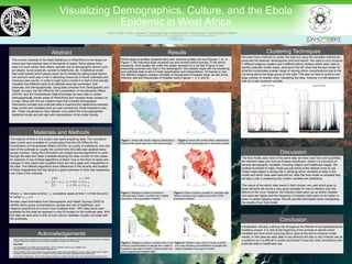
We used many methods to cluster the data but using the complete method we
produced the cleanest dendrograms (pictured below). We used a cut to produce
7 different religious clusters and 9 different ethnic clusters which were used to
identify culturally similar areas, pictured to the left. Note that the last cluster for
ethnicity incorporates a wider range of varying ethnic concentrations due to the
cut being above the large group on the right. This was cut here to avoid a very
large number of clusters when visualizing the data, however it is still apparent
that not a well clustered variable.
1. Department of Mathematics, 2. Department of Statistical Science, 3. Center for Modeling Complex Interactions
*aranb@uidaho.edu
**mwiest@uidaho.edu
Figure 1: Areas with similar religious distributions.
Points of the same type are in the same cluster
Figure 2: Areas with similar ethnic distributions.
Points of the same type are in the same cluster
Figure 3: Religious clusters overlaid on
outbreak data. Darker counties had a higher
proportion of the population infected
Figure 4: Ethnic clusters overlaid on outbreak data.
Darker counties had a higher proportion of the
population infected
Figure 4: Religious clusters overlaid onto a map
showing concentrations of people who visited a
hospital in the past 6 months. Darker areas had
more proportional hospital visits.
Figure 6: Infection rates (size of circle) overlaid
onto map showing concentrations of people who
visited hospitals in the past 6 months.
The final model uses most of the same data we have used here and quantifies
the infection rates over time as Poisson distribution, where λ is a function of
several demographic variables, including religion and healthcare usage. We
created hundreds of maps; these are just some of the clearest ones to use.
These maps played a strong role in deciding which variables to keep in the
model and which ones were best left out. After the final model is complete they
will play a role in explaining why certain variables are predictors.
The nature of the ethnic data meant it didn’t cluster very well which goes to
show ethnicity will not be a very good correlate for risk of infection over the
lifetime of the virus. However, the infection rates seem go up where hospital
visit rates are higher and the frequency of hospital visits seem to be higher or
lower in certain religious areas. We will use this information when interpreting
the results of our final model.
Cut
Cut
While religious profiles clustered fairly well, ethnicity profiles did not (Figures 7, 8). In
Figure 7, the individual sites clustered low and formed distinct groups. In the ethnic
clustering, most locales fell under the cluster denoted by a red star (Figure 2) and
branching occurred very high in the dendrogram. We created maps with the clustering
and outbreak data to aid in model specification and interpretation. Of interest is how
the different religious clusters correlate to frequencies of hospital visits, as well at the
infection rate and frequencies of hospital visits (Figures 1, 3, 4, and 6).
0 - 0.46
0.47 - 1.91
1.92 – 4.20
4.21 – 10.01
10.02 – 18.31
18.32 – 37.80
37.81 – 61.55
0 - 0.46
0.47 - 1.91
1.92 – 4.20
4.21 – 10.01
10.02 – 18.31
18.32 – 37.80
37.81 – 61.55
0 - 0.46
0.47 - 1.91
1.92 – 4.20
4.21 – 10.01
10.02 – 18.31
18.32 – 37.80
37.81 – 61.55
Infection
Rates per
10,000
Infection
Rates per
10,000
Infection
Rates per
10,000