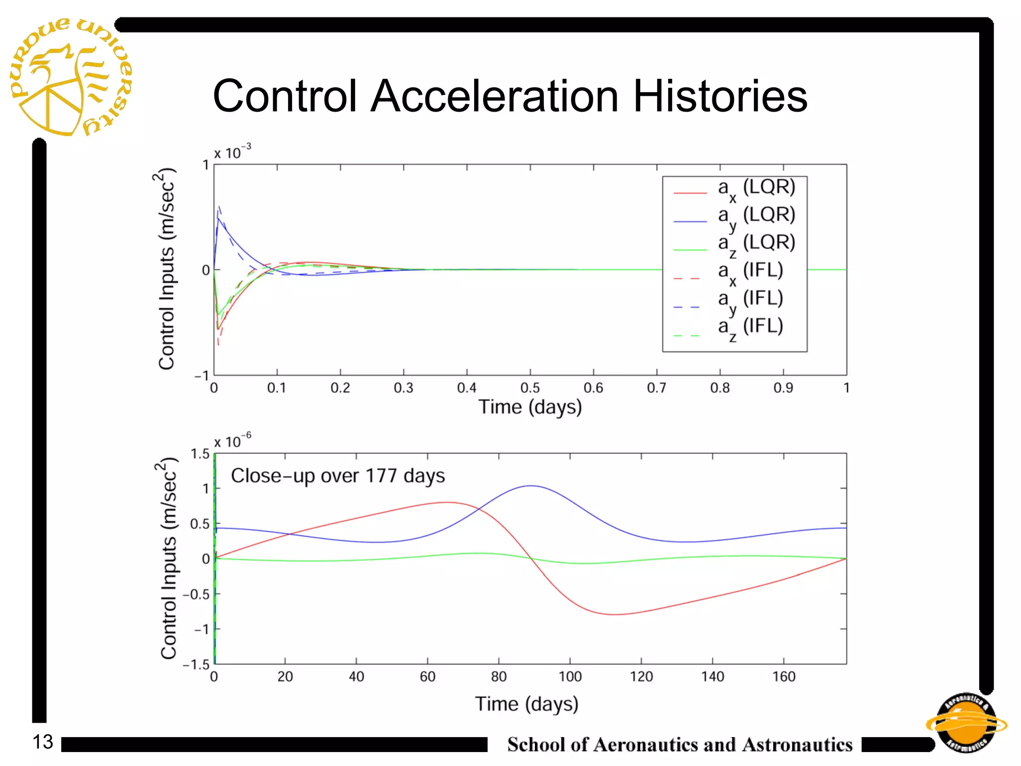
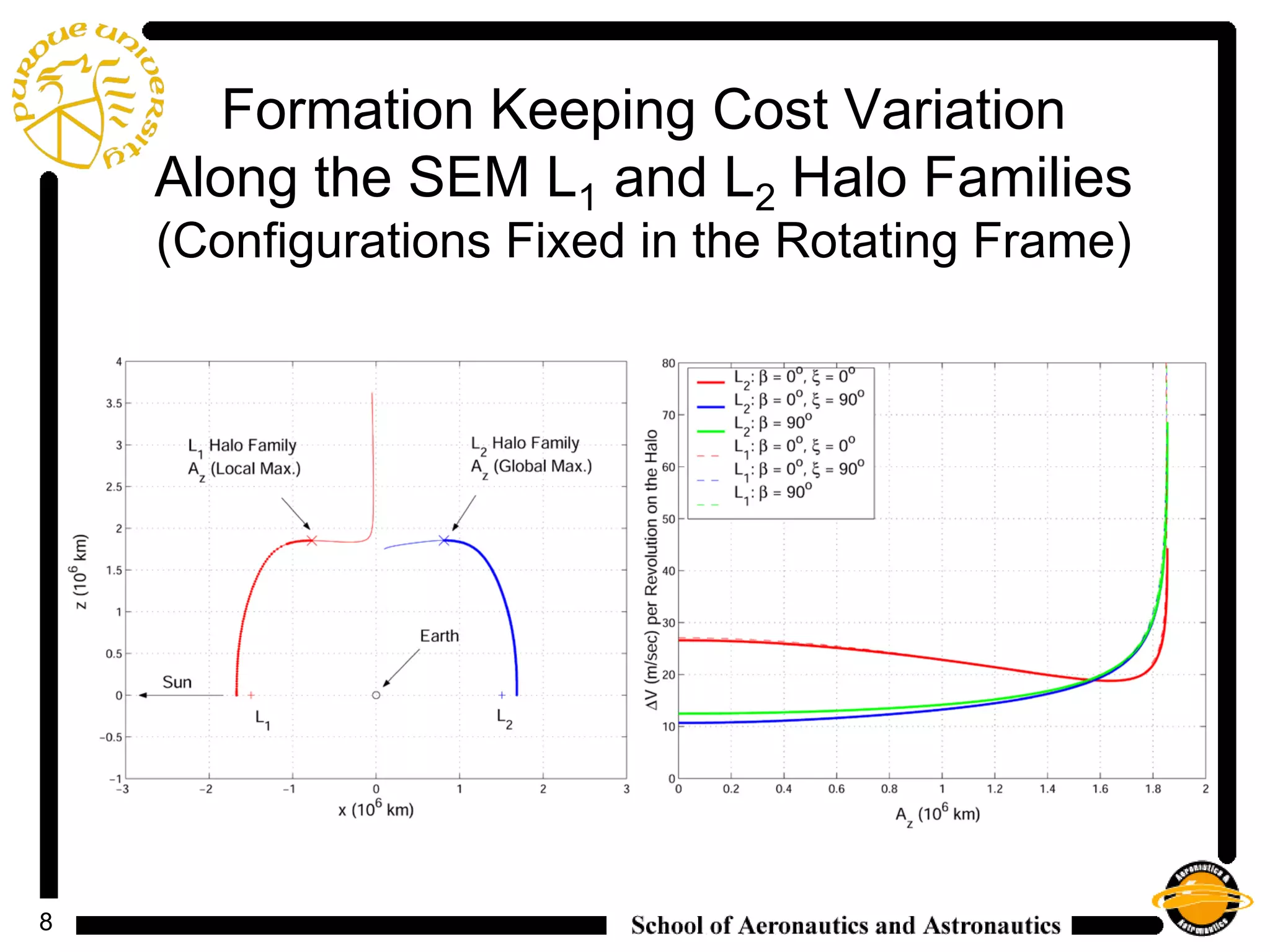
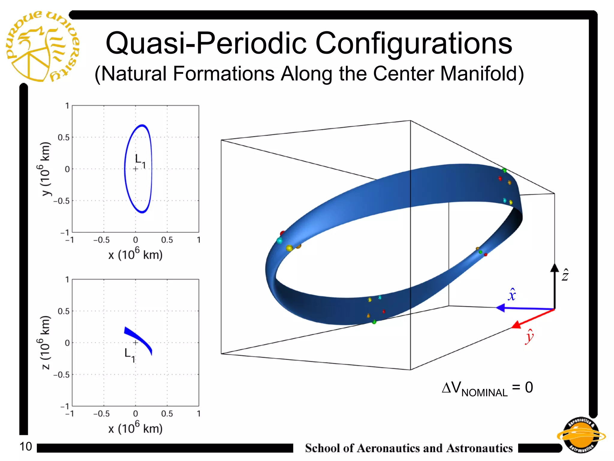
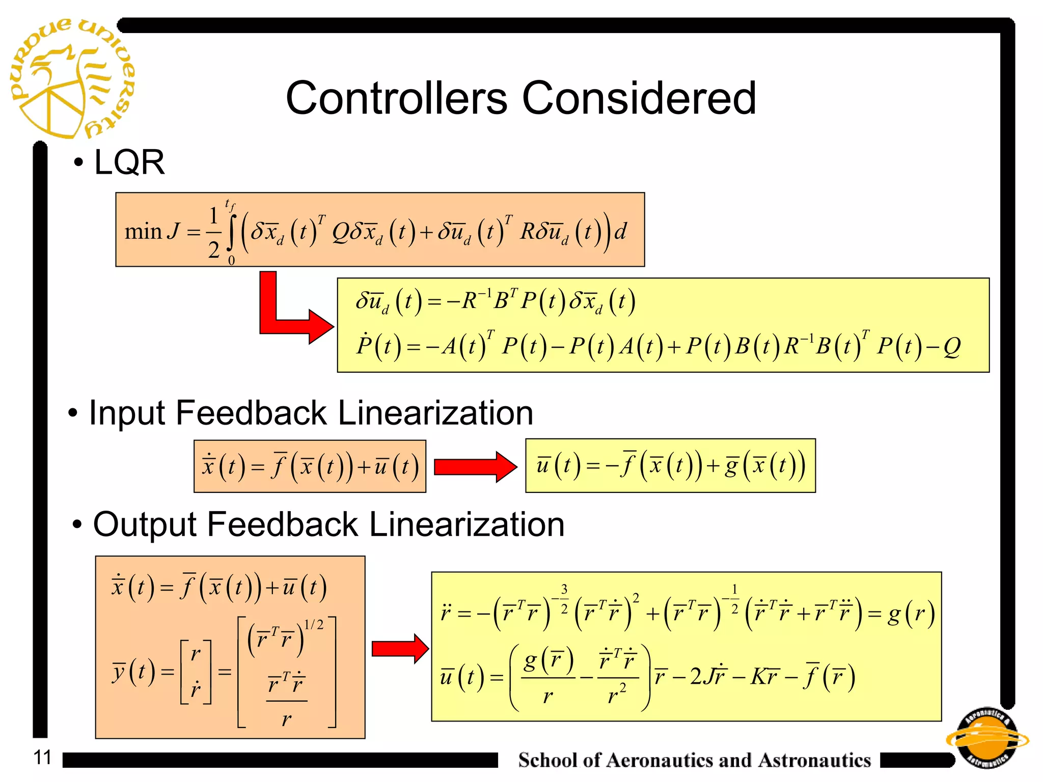
1) The document discusses control strategies for maintaining spacecraft formations near libration points using linear quadratic regulator (LQR) and input feedback linearization (IFL) controllers. 2) It analyzes the costs and control histories for formations with different configurations fixed in the rotating frame, finding that natural formations have very low nominal costs and that LQR and IFL controllers effectively stabilize formations above this nominal cost. 3) While control accelerations required are extremely low, complexity increases when transferring the results to an ephemeris model that includes additional sources of error and uncertainty.

1. 1
CONTROL STRATEGIES FOR FORMATION FLIGHT
IN THE VICINITY OF THE LIBRATION POINTS
K.C. Howell and B.G. Marchand
Purdue University

2. 2
Previous Work on Formation Flight
• Multi-S/C Formations in the 2BP
– Small Relative Separation (10 m – 1 km)
• Model Relative Dynamics via the C-W Equations
• Formation Control
– LQR for Time Invariant Systems
– Feedback Linearization
– Lyapunov Based and Adaptive Control
• Multi-S/C Formations in the 3BP
– Consider Wider Separation Range
• Nonlinear model with complex reference motions
– Periodic, Quasi-Periodic, Stable/Unstable Manifolds
• Formation Control via simplified LQR techniques
and “Gain Scheduling”-type methods.

3. 3
Deputy S/C
( ), ,d d dx y z
ˆx
ˆy
2-S/C Formation Model
in the Sun-Earth-Moon System
ˆX
ˆ ˆ,Z z
B
1cr
2crcr
ˆxθ
ˆy
Chief S/C
( ), ,c c cx y z
ˆdr rρ=
ˆr
ξ
β

4. 4
Dynamical Model
( ) ( ) ( ) ( ) ( )
( ) ( ) ( ) ( ) ( ) ( ) ( )
2
2
c c c c c
d c d c d d d
r t f r t Jr t Kr t u t
r t f r t r t f r t Jr t Kr t u t
= + + +  
= + − + + +      
 
 
Nonlinear EOMs:
( ) ( )
( ) ( ) ( ) ( )( )
( ) ( )
( ) ( )
( ) ( )( )
0 0
, 2
d d d d
d d
c dd d d d
Ir t r t r t r t
u t u t
r t r t J Ir t r t r t r t
    − −  
+ −      Ω− −       
 

 
 
   
Linear System:
( )A t B ( )du tδ( )dx tδ( )dx tδ 

5. 5
Reference Motions
• Fixed Relative Distance and Orientation
– Chief-Deputy Line Fixed Relative to the Rotating Frame
– Chief-Deputy Line Fixed Relative to the Inertial Frame
• Fixed Relative Distance, No Orientation Constraints
• Natural Formations (Center Manifold)
– Deputy evolves along a quasi-periodic 2-D Torus that
envelops the chief spacecraft’s halo orbit (bounded motion)
( ) ( )and 0d dr t c r t= =
( )
( )
( )
0 0
0 0
0
cos sin
cos sin
d d d
d d d
d d
x t x t y t
y t y t x t
z t z
= +
= −
=

6. 6
Nominal Formation Keeping Cost
(Configurations Fixed in the Rotating Frame)
Az = 0.2×106 km
Az = 1.2×106 km
Az = 0.7×106 km
5000 kmρ =

7. 7
Max./Min. Cost Formations
(Configurations Fixed in the Rotating Frame)
ˆx
Deputy S/C
Deputy S/C
Deputy S/C
Deputy S/C
Chief S/C
ˆy
ˆz
Minimum Cost Formations
ˆz
ˆy
ˆx
Deputy S/C
Deputy S/CChief S/C
Maximum Cost Formation

8. 8
Formation Keeping Cost Variation
Along the SEM L1 and L2 Halo Families
(Configurations Fixed in the Rotating Frame)

9. 9
Nominal Formation Keeping Cost
(Configurations Fixed in the Rotating Frame)
Az = 0.2×106 km
Az = 1.2×106 km
Az = 0.7×106 km

10. 10
Quasi-Periodic Configurations
(Natural Formations Along the Center Manifold)
ˆx
ˆy
ˆz
∆VNOMINAL = 0

11. 11
Controllers Considered
( ) ( ) ( ) ( )( )0
1
min
2
ft
T T
d d d dJ x t Q x t u t R u t d tδ δ δ δ+∫
• LQR
( ) ( )( ) ( )x t f x t u t= + ( ) ( )( ) ( )( )u t f x t g x t=− +
• Input Feedback Linearization
( ) ( )( ) ( )
( )
( )
1/2T
T
x t f x t u t
r r
r
y t
r rr
r
= +
 
  
= =   
   
 


( ) ( ) ( ) ( ) ( )
( )
( )
( )
3 1
2
2 2
2
2
T T T T T
T
r r r r r r r r r r r g r
g r r r
u t r Jr Kr f r
r r
− −
=− + + =
 
= − − − − 
 
   
 

• Output Feedback Linearization
( ) ( ) ( )
( ) ( ) ( ) ( ) ( ) ( ) ( ) ( ) ( )
1
1
T
d d
T T
u t R B P t x t
P t A t P t P t A t P t B t R B t P t Q
δ δ−
−
= −
=− − + −

12. 12
Dynamic Response to Injection Error
5000 km, 90 , 0ρ ξ β= = = 
LQR Controller IFL Controller
( ) [ ]0 7 km 5 km 3.5 km 1 mps 1 mps 1 mps
T
xδ =− −

13. 13
Control Acceleration Histories

14. 14
Conclusions
• Natural vs. Forced Formations
– The nominal formation keeping costs in the CR3BP are very
low, even for relatively large non-naturally occurring formations.
• Above the nominal cost, standard LQR and FL
approaches work well in this problem.
– Both LQR & FL yield essentially the same control histories but
FL method is computationally simpler to implement.
• The required control accelerations are extremely low.
However, this may change once other sources of error
and uncertainty are introduced.
– Low Thrust Delivery
– Continuous vs. Discrete Control
• Complexity increases once these results are transferred
into the ephemeris model.