sjdndn

1. © 2009 South-Western, a part of Cengage Learning, all rights reserved
C H A P T E R
Firms in Competitive Markets
Firms in Competitive Markets
Microeonomics
P R I N C I P L E S O F
P R I N C I P L E S O F
N. Gregory
N. Gregory
Mankiw
Mankiw
Premium PowerPoint Slides
by Ron Cronovich
14

2. In this chapter,
In this chapter,
look for the answers to these questions:
look for the answers to these questions:
 What is a perfectly competitive market?
 What is marginal revenue? How is it related to total
and average revenue?
 How does a competitive firm determine the quantity
that maximizes profits?
 When might a competitive firm shut down in the
short run? Exit the market in the long run?
 What does the market supply curve look like in the
short run? In the long run?
2

3. FIRMS IN COMPETITIVE MARKETS 3
Introduction: A Scenario
 Three years after graduating, you run your own
business.
 You must decide how much to produce, what price
to charge, how many workers to hire, etc.
 What factors should affect these decisions?
 Your costs (studied in previous chapter)
 How much competition you face
 We begin by studying the behavior of firms in
perfectly competitive markets.

4. FIRMS IN COMPETITIVE MARKETS 4
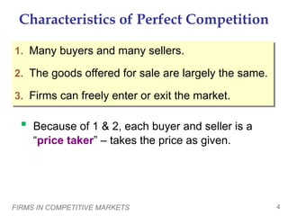
Characteristics of Perfect Competition
1. Many buyers and many sellers.
2. The goods offered for sale are largely the same.
3. Firms can freely enter or exit the market.
 Because of 1 & 2, each buyer and seller is a
“price taker” – takes the price as given.

5. FIRMS IN COMPETITIVE MARKETS 5
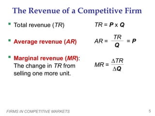
The Revenue of a Competitive Firm
 Total revenue (TR)
 Average revenue (AR)
 Marginal revenue (MR):
The change in TR from
selling one more unit.
∆TR
∆Q
MR =
TR = P x Q
TR
Q
AR = = P

6. A C T I V E L E A R N I N G
A C T I V E L E A R N I N G 1
1
Calculating
Calculating TR
TR,
, AR
AR,
, MR
MR
6
Fill in the empty spaces of the table.
50
10
5
40
10
4
10
3
10
2
10
10
1
n/a
10
0
TR
P
Q MR
AR
10

7. A C T I V E L E A R N I N G
A C T I V E L E A R N I N G 1
1
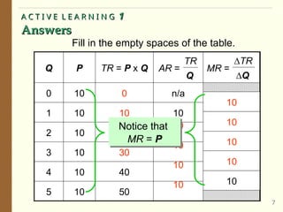
Answers
Answers
7
Fill in the empty spaces of the table.
50
10
5
40
10
4
10
3
10
10
10
10
10
2
10
10
1
n/a
30
20
10
0
10
0
TR = P x Q
P
Q
∆TR
∆Q
MR =
TR
Q
AR =
10
10
10
10
10
Notice that
MR = P

8. FIRMS IN COMPETITIVE MARKETS 8
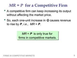
MR = P for a Competitive Firm
 A competitive firm can keep increasing its output
without affecting the market price.
 So, each one-unit increase in Q causes revenue
to rise by P, i.e., MR = P.
MR = P is only true for
firms in competitive markets.

9. FIRMS IN COMPETITIVE MARKETS 9
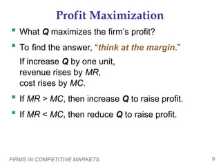
Profit Maximization
 What Q maximizes the firm’s profit?
 To find the answer, “think at the margin.”
If increase Q by one unit,
revenue rises by MR,
cost rises by MC.
 If MR > MC, then increase Q to raise profit.
 If MR < MC, then reduce Q to raise profit.

10. FIRMS IN COMPETITIVE MARKETS 10
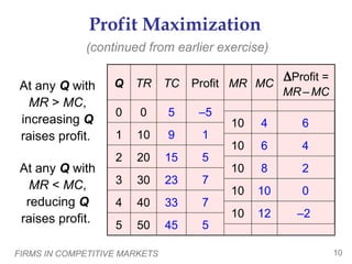
Profit Maximization
50
5
40
4
30
3
20
2
10
1
45
33
23
15
9
5
0
0
Profit =
MR – MC
MC
MR
Profit
TC
TR
Q
At any Q with
MR > MC,
increasing Q
raises profit.
5
7
7
5
1
–5
10
10
10
10
–2
0
2
4
6
12
10
8
6
4
10
(continued from earlier exercise)
At any Q with
MR < MC,
reducing Q
raises profit.

11. FIRMS IN COMPETITIVE MARKETS 11
P1 MR
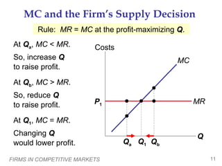
MC and the Firm’s Supply Decision
At Qa, MC < MR.
So, increase Q
to raise profit.
At Qb, MC > MR.
So, reduce Q
to raise profit.
At Q1, MC = MR.
Changing Q
would lower profit.
Q
Costs
MC
Q1
Qa Qb
Rule: MR = MC at the profit-maximizing Q.

12. FIRMS IN COMPETITIVE MARKETS 12
P1 MR
P2 MR2
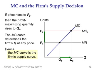
MC and the Firm’s Supply Decision
If price rises to P2,
then the profit-
maximizing quantity
rises to Q2.
The MC curve
determines the
firm’s Q at any price.
Hence,
Q
Costs
MC
Q1 Q2
the MC curve is the
firm’s supply curve.

13. FIRMS IN COMPETITIVE MARKETS 13
Shutdown vs. Exit
 Shutdown:
A short-run decision not to produce anything
because of market conditions.
 Exit:
A long-run decision to leave the market.
 A key difference:
 If shut down in SR, must still pay FC.
 If exit in LR, zero costs.

14. FIRMS IN COMPETITIVE MARKETS 14
A Firm’s Short-run Decision to Shut Down
 Cost of shutting down: revenue loss = TR
 Benefit of shutting down: cost savings = VC
(firm must still pay FC)
 So, shut down if TR < VC
 Divide both sides by Q: TR/Q < VC/Q
 So, firm’s decision rule is:
Shut down if P < AVC

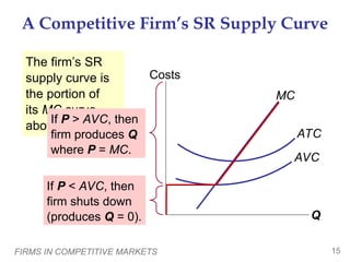
15. FIRMS IN COMPETITIVE MARKETS 15
The firm’s SR
supply curve is
the portion of
its MC curve
above AVC.
Q
Costs
A Competitive Firm’s SR Supply Curve
MC
ATC
AVC
If P > AVC, then
firm produces Q
where P = MC.
If P < AVC, then
firm shuts down
(produces Q = 0).

16. FIRMS IN COMPETITIVE MARKETS 16
The Irrelevance of Sunk Costs
 Sunk cost: a cost that has already been
committed and cannot be recovered
 Sunk costs should be irrelevant to decisions;
you must pay them regardless of your choice.
 FC is a sunk cost: The firm must pay its fixed
costs whether it produces or shuts down.
 So, FC should not matter in the decision to shut
down.

17. FIRMS IN COMPETITIVE MARKETS 17
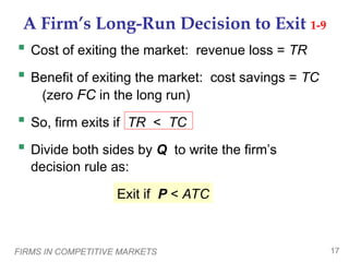
A Firm’s Long-Run Decision to Exit 1-9
 Cost of exiting the market: revenue loss = TR
 Benefit of exiting the market: cost savings = TC
(zero FC in the long run)
 So, firm exits if TR < TC
 Divide both sides by Q to write the firm’s
decision rule as:
Exit if P < ATC

18. FIRMS IN COMPETITIVE MARKETS 18
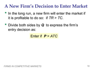
A New Firm’s Decision to Enter Market
 In the long run, a new firm will enter the market if
it is profitable to do so: if TR > TC.
 Divide both sides by Q to express the firm’s
entry decision as:
Enter if P > ATC

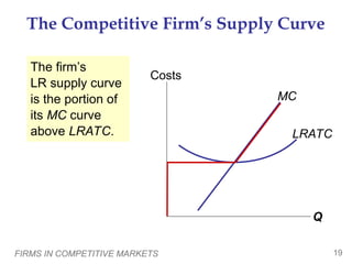
19. FIRMS IN COMPETITIVE MARKETS 19
The firm’s
LR supply curve
is the portion of
its MC curve
above LRATC.
Q
Costs
The Competitive Firm’s Supply Curve
MC
LRATC

20. A C T I V E L E A R N I N G
A C T I V E L E A R N I N G 2
2
Identifying a firm’s profit
Identifying a firm’s profit
20
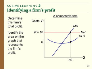
Determine
this firm’s
total profit.
Identify the
area on the
graph that
represents
the firm’s
profit.
Q
Costs, P
MC
ATC
P = 10 MR
50
6
A competitive firm

21. A C T I V E L E A R N I N G
A C T I V E L E A R N I N G 2
2
Answers
Answers
21
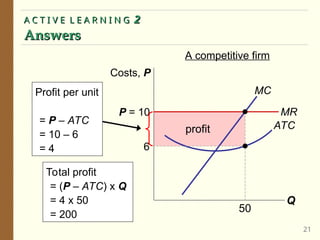
profit
Q
Costs, P
MC
ATC
P = 10 MR
50
6
A competitive firm
Profit per unit
= P – ATC
= 10 – 6
= 4
Total profit
= (P – ATC) x Q
= 4 x 50
= 200

22. A C T I V E L E A R N I N G
A C T I V E L E A R N I N G 3
3
Identifying a firm’s loss
Identifying a firm’s loss
22
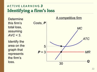
Determine
this firm’s
total loss,
assuming
AVC < 3.
Identify the
area on the
graph that
represents
the firm’s
loss. Q
Costs, P
MC
ATC
A competitive firm
5
P = 3 MR
30

23. A C T I V E L E A R N I N G
A C T I V E L E A R N I N G 3
3
Answers
Answers
23
loss
MR
P = 3
Q
Costs, P
MC
ATC
A competitive firm
loss per unit = 2
Total loss
= (ATC – P) x Q
= 2 x 30
= 60
5
30

24. FIRMS IN COMPETITIVE MARKETS 24
Market Supply: Assumptions
1) All existing firms and potential entrants have
identical costs.
2) Each firm’s costs do not change as other firms
enter or exit the market.
3) The number of firms in the market is
 fixed in the short run
(due to fixed costs)
 variable in the long run
(due to free entry and exit)

25. FIRMS IN COMPETITIVE MARKETS 25
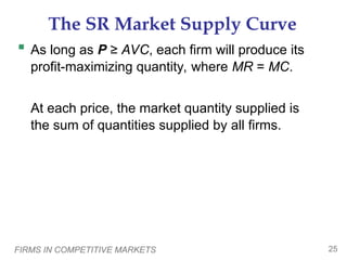
The SR Market Supply Curve
 As long as P ≥ AVC, each firm will produce its
profit-maximizing quantity, where MR = MC.
At each price, the market quantity supplied is
the sum of quantities supplied by all firms.

26. FIRMS IN COMPETITIVE MARKETS 26
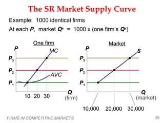
The SR Market Supply Curve
MC
P2
Market
Q
P
(market)
One firm
Q
P
(firm)
S
P3
Example: 1000 identical firms
At each P, market Qs
= 1000 x (one firm’s Qs
)
AVC
P2
P3
30
P1
20
10
P1
30,000
10,000 20,000

27. FIRMS IN COMPETITIVE MARKETS 27
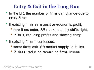
Entry & Exit in the Long Run
 In the LR, the number of firms can change due to
entry & exit.
 If existing firms earn positive economic profit,
 new firms enter, SR market supply shifts right.
 P falls, reducing profits and slowing entry.
 If existing firms incur losses,
 some firms exit, SR market supply shifts left.
 P rises, reducing remaining firms’ losses.

28. FIRMS IN COMPETITIVE MARKETS 28
The Zero-Profit Condition
 Long-run equilibrium:
The process of entry or exit is complete –
remaining firms earn zero economic profit.
 Zero economic profit occurs when P = ATC.
 Since firms produce where P = MR = MC,
the zero-profit condition is P = MC = ATC.
 Since, that MC intersects ATC at minimum ATC.
 Hence, in the long run, P = minimum ATC.

29. FIRMS IN COMPETITIVE MARKETS 29
Why Do Firms Stay in Business if Profit = 0?
 Economic profit is revenue minus all costs –
including implicit costs, like the opportunity cost
of the owner’s time and money.
 In the zero-profit equilibrium,
 firms earn enough revenue to cover these costs
 accounting profit is positive

30. FIRMS IN COMPETITIVE MARKETS 30
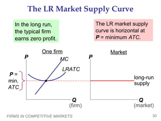
The LR Market Supply Curve
MC
Market
Q
P
(market)
One firm
Q
P
(firm)
In the long run,
the typical firm
earns zero profit.
LRATC
long-run
supply
P =
min.
ATC
The LR market supply
curve is horizontal at
P = minimum ATC.

31. FIRMS IN COMPETITIVE MARKETS 31
S1
Profit
D1
P1
long-run
supply
D2
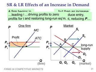
SR & LR Effects of an Increase in Demand
MC
ATC
P1
Market
Q
P
(market)
One firm
Q
P
(firm)
P2
P2
Q1 Q2
S2
Q3
A firm begins in
long-run eq’m…
…but then an increase
in demand raises P,…
…leading to SR
profits for the firm.
Over time, profits induce entry,
shifting S to the right, reducing P…
…driving profits to zero
and restoring long-run eq’m.
A
B
C

32. FIRMS IN COMPETITIVE MARKETS 32
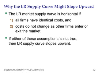
Why the LR Supply Curve Might Slope Upward
 The LR market supply curve is horizontal if
1) all firms have identical costs, and
2) costs do not change as other firms enter or
exit the market.
 If either of these assumptions is not true,
then LR supply curve slopes upward.

33. FIRMS IN COMPETITIVE MARKETS 33
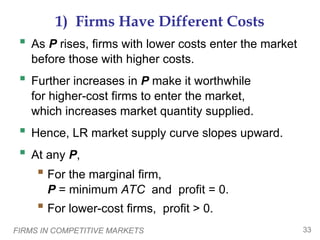
1) Firms Have Different Costs
 As P rises, firms with lower costs enter the market
before those with higher costs.
 Further increases in P make it worthwhile
for higher-cost firms to enter the market,
which increases market quantity supplied.
 Hence, LR market supply curve slopes upward.
 At any P,
 For the marginal firm,
P = minimum ATC and profit = 0.
 For lower-cost firms, profit > 0.

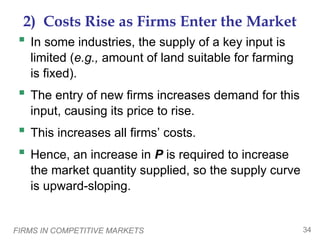
34. FIRMS IN COMPETITIVE MARKETS 34
2) Costs Rise as Firms Enter the Market
 In some industries, the supply of a key input is
limited (e.g., amount of land suitable for farming
is fixed).
 The entry of new firms increases demand for this
input, causing its price to rise.
 This increases all firms’ costs.
 Hence, an increase in P is required to increase
the market quantity supplied, so the supply curve
is upward-sloping.

35. FIRMS IN COMPETITIVE MARKETS 35
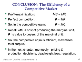
CONCLUSION: The Efficiency of a
Competitive Market
 Profit-maximization: MC = MR
 Perfect competition: P = MR
 So, in the competitive eq’m: P = MC
 Recall, MC is cost of producing the marginal unit.
P is value to buyers of the marginal unit.
 So, the competitive eq’m is efficient, maximizes
total surplus.
 In the next chapter, monopoly: pricing &
production decisions, deadweight loss, regulation.

36. CHAPTER SUMMARY
CHAPTER SUMMARY
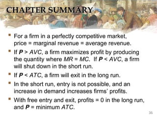
 For a firm in a perfectly competitive market,
price = marginal revenue = average revenue.
 If P > AVC, a firm maximizes profit by producing
the quantity where MR = MC. If P < AVC, a firm
will shut down in the short run.
 If P < ATC, a firm will exit in the long run.
 In the short run, entry is not possible, and an
increase in demand increases firms’ profits.
 With free entry and exit, profits = 0 in the long run,
and P = minimum ATC.
36