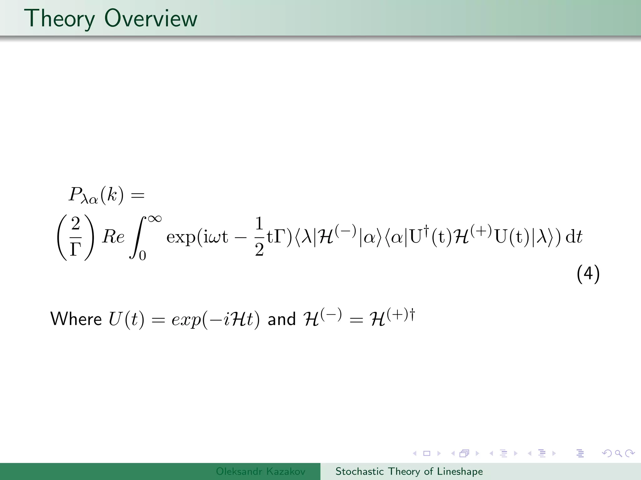
The document describes an algorithm for simulating stochastic lineshapes using a multidimensional array approach. It involves:
1. Generating a 6D array to represent the Liouville matrix and casting it into a 2D array.
2. Inverting the 2D array and casting it back to 6D.
3. Using indexing methods to reference elements between the 2D and 6D arrays and perform summations to calculate lineshapes.
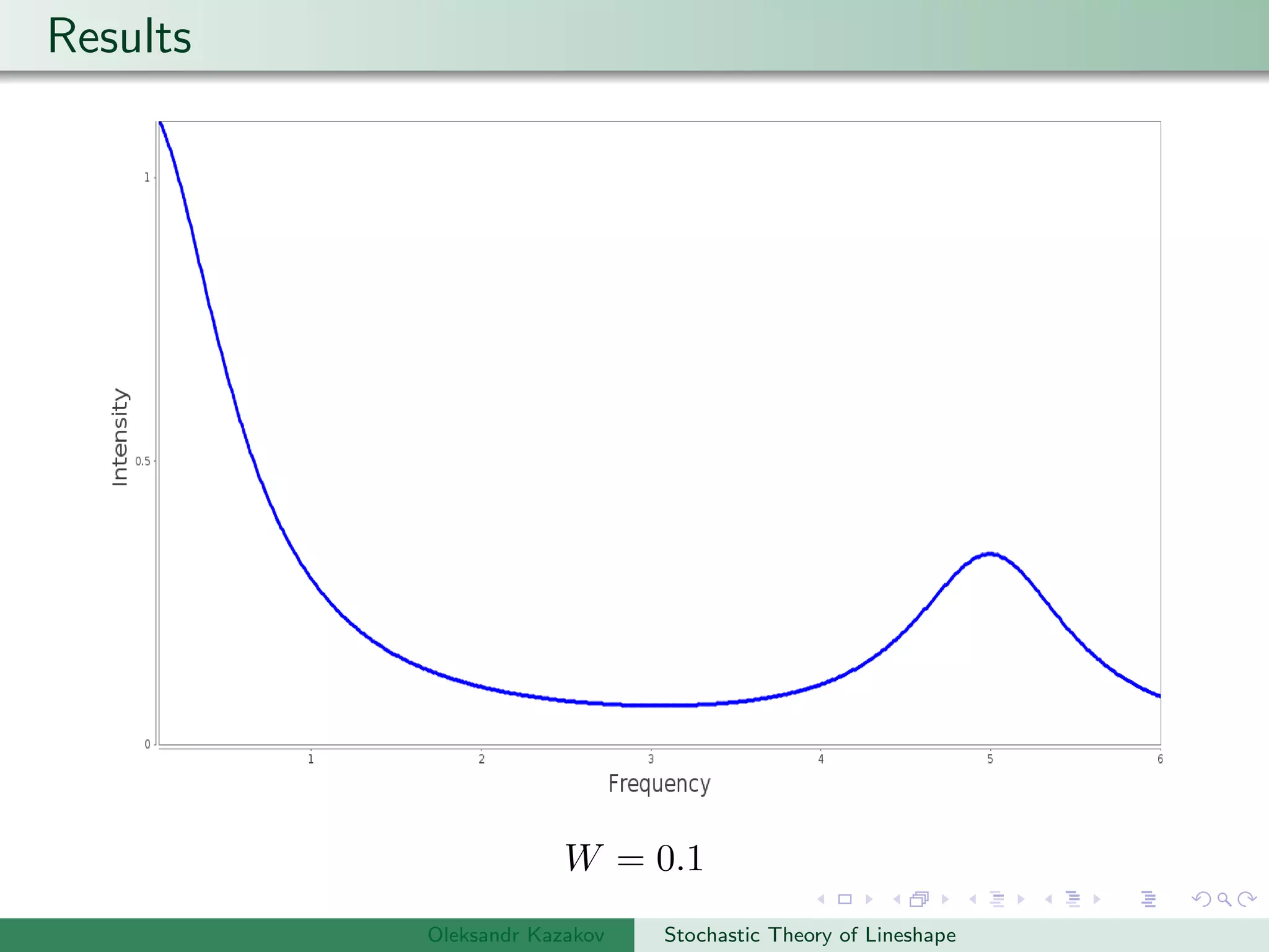
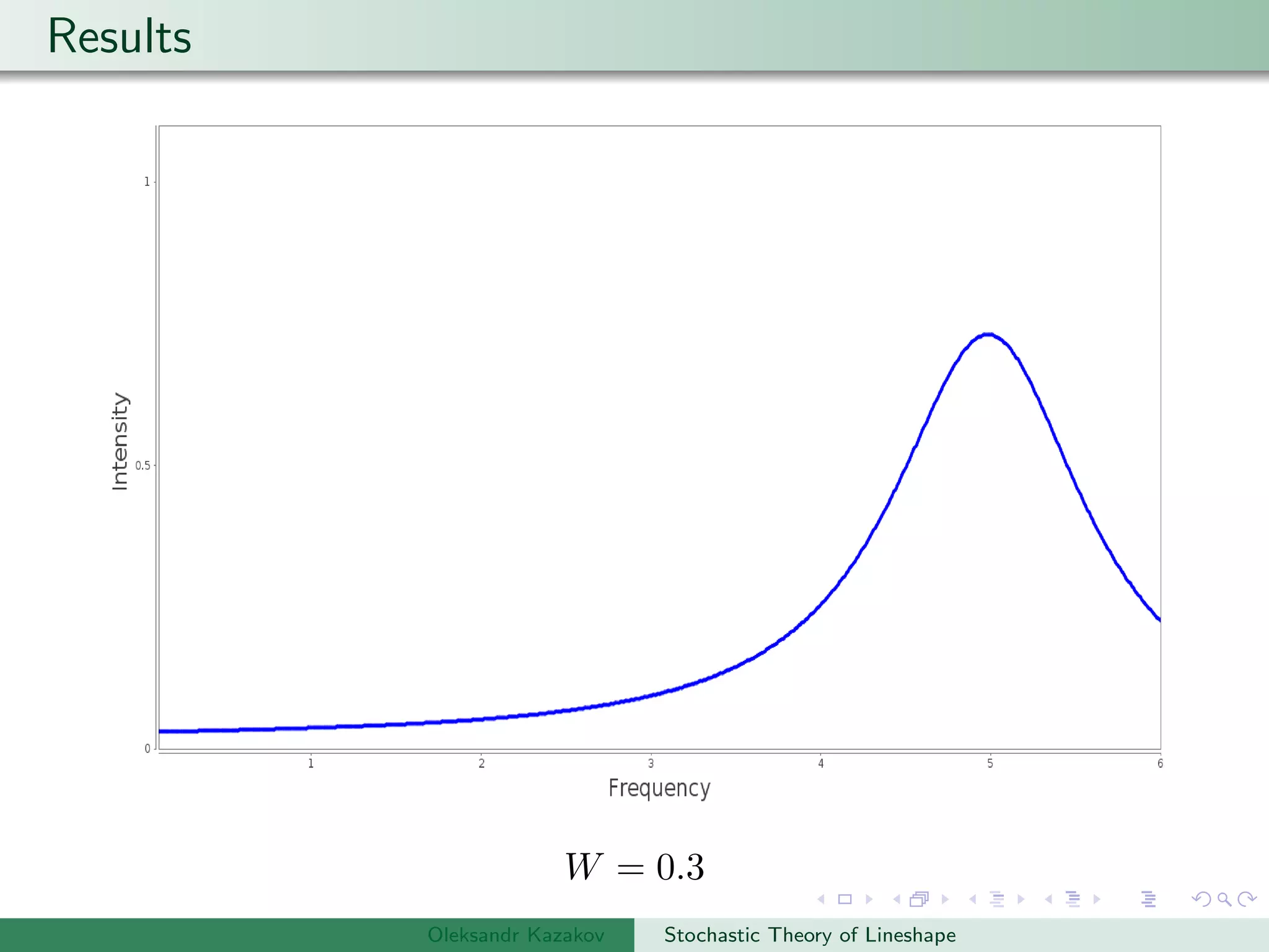
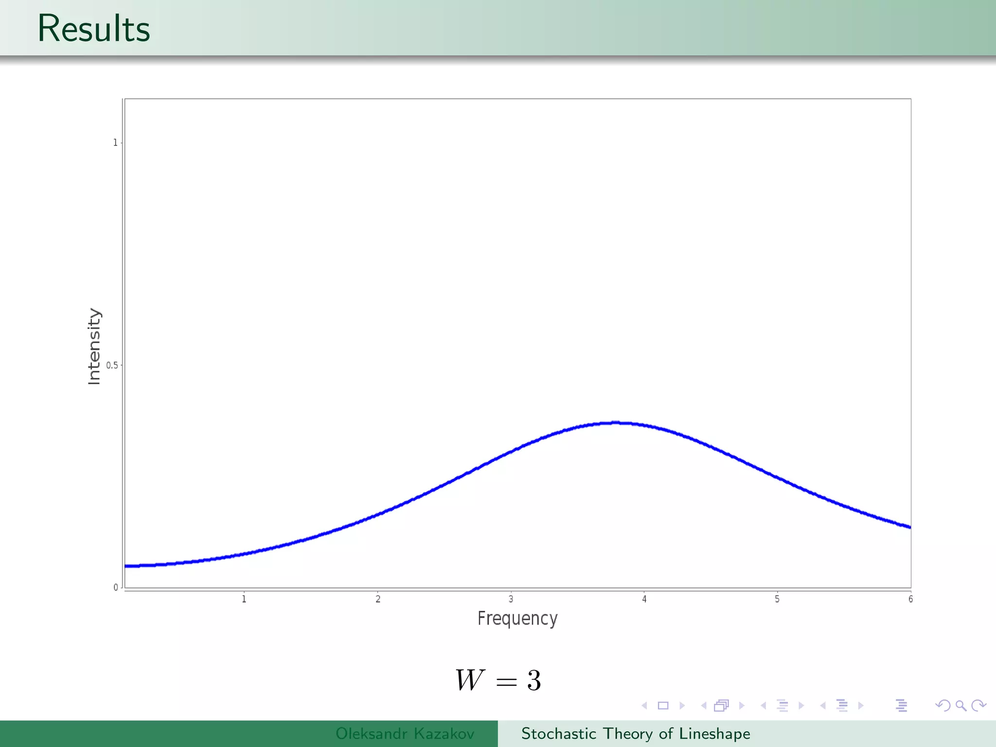
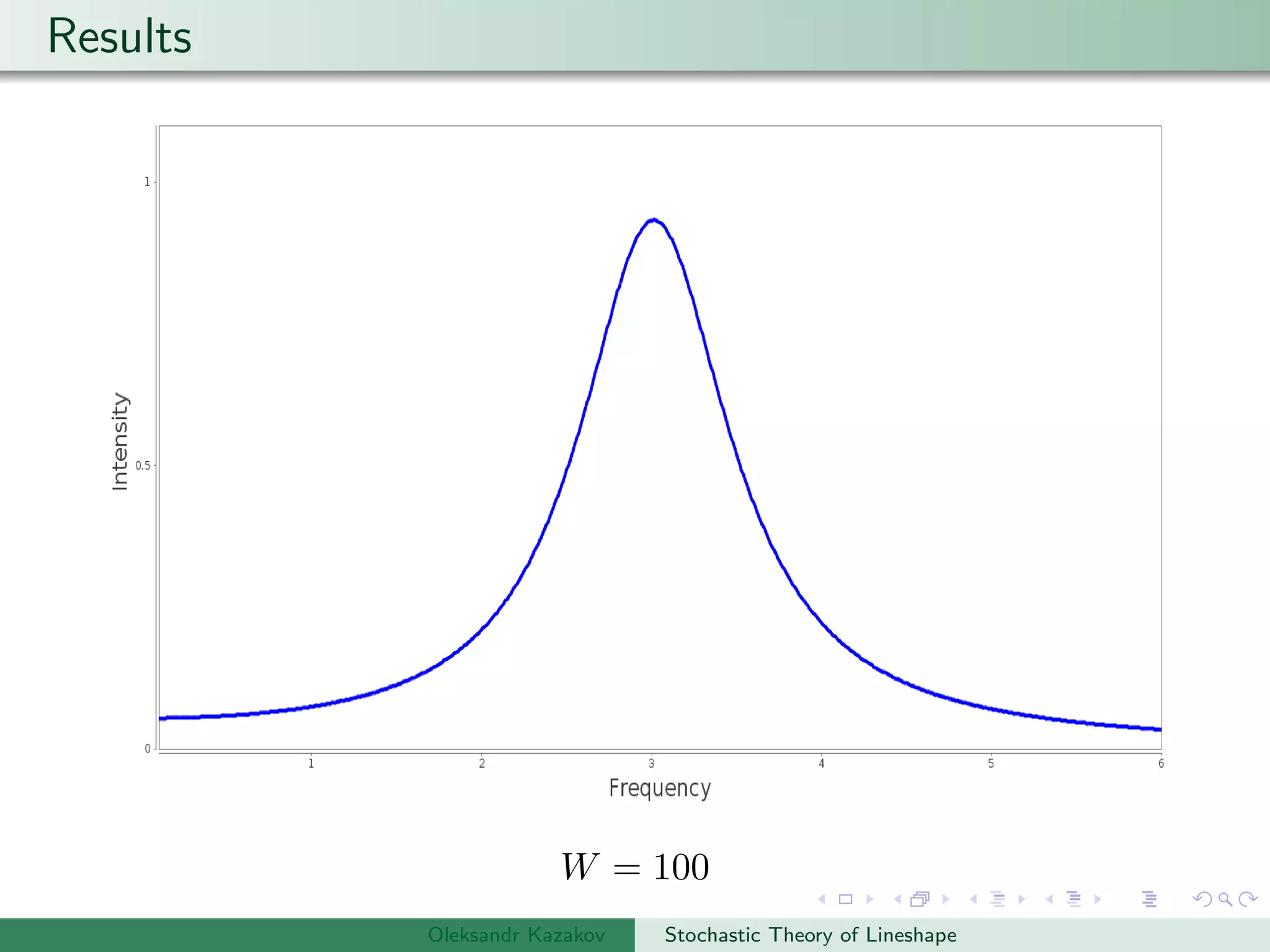
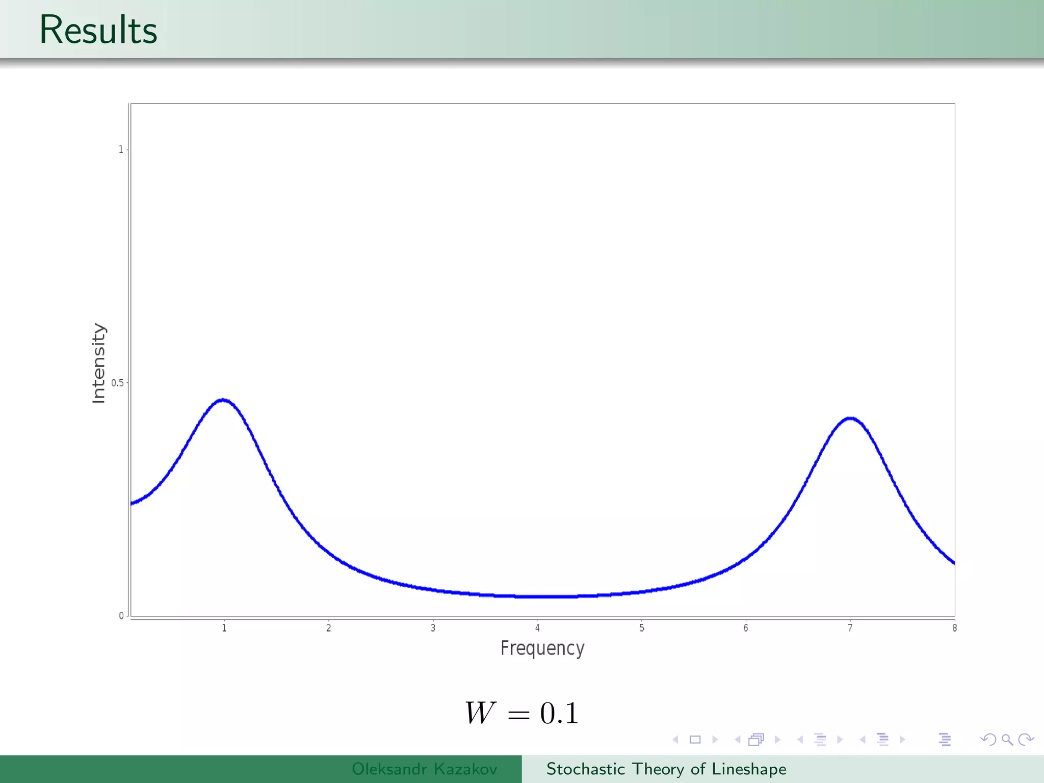
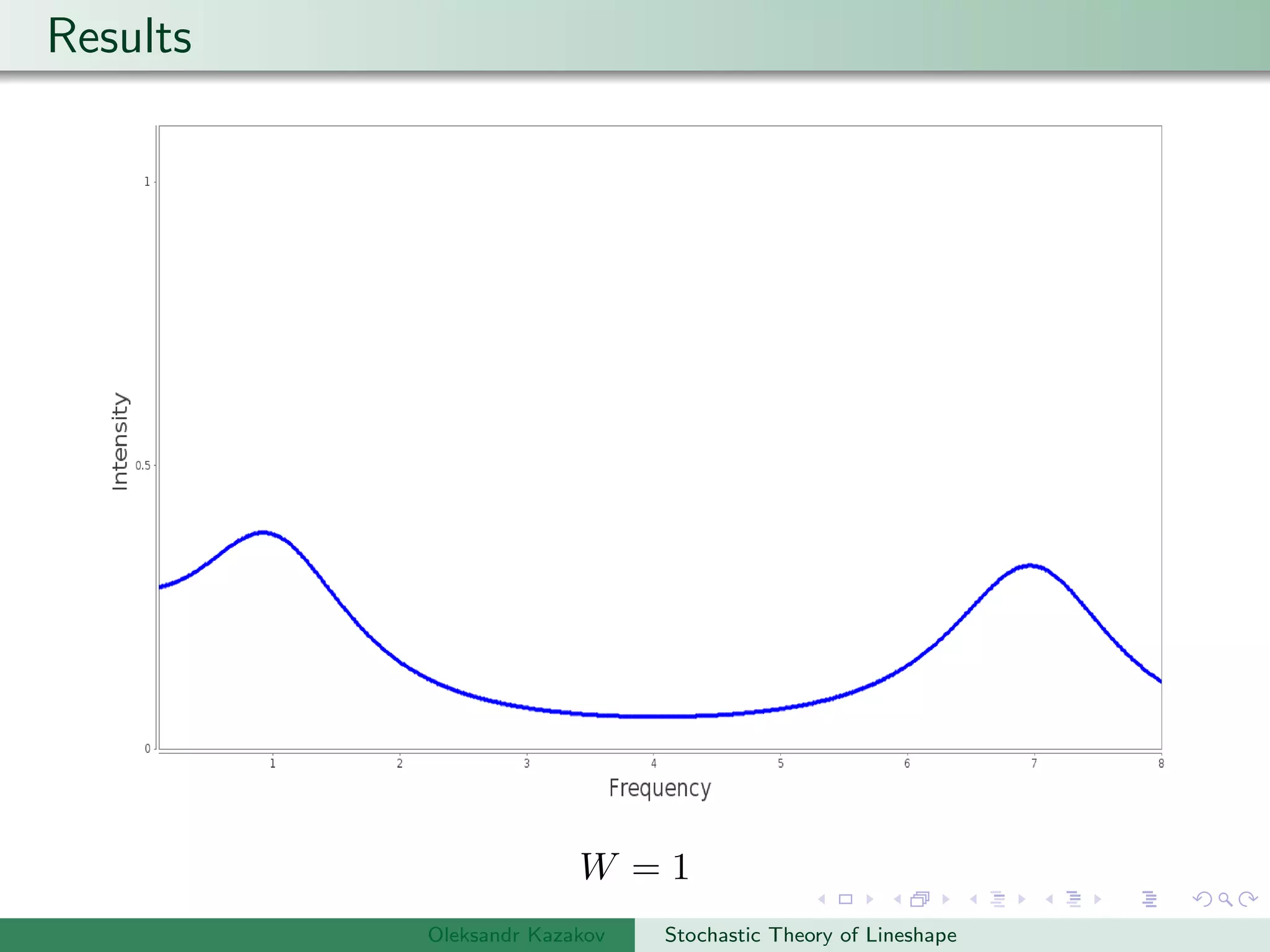
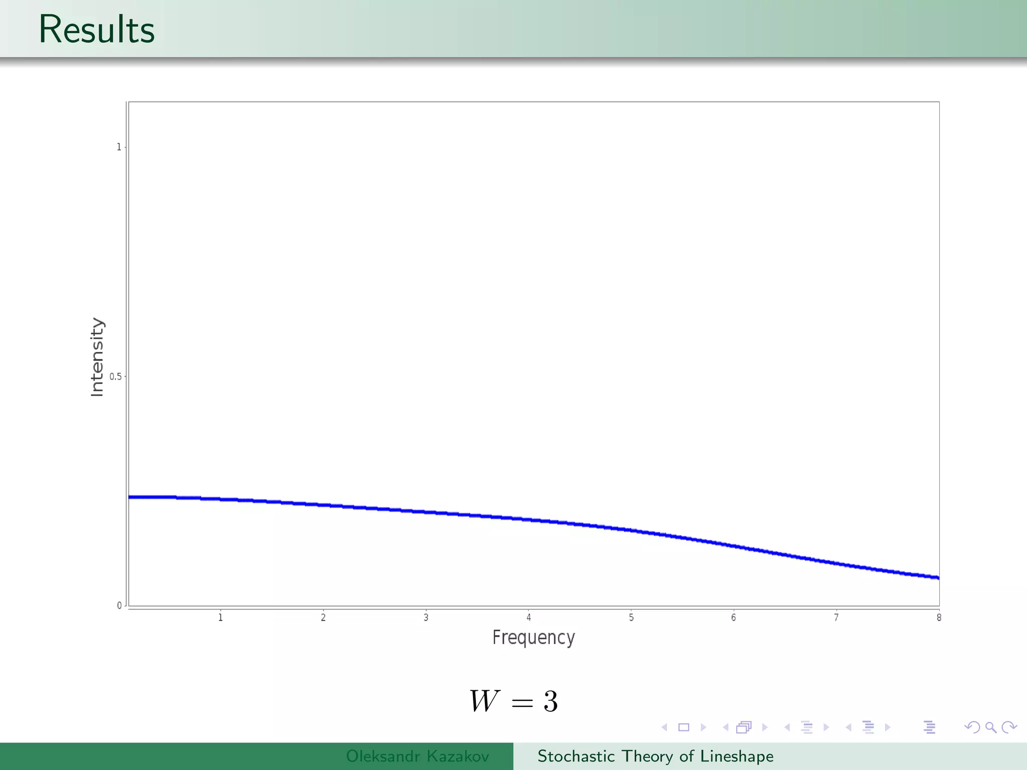
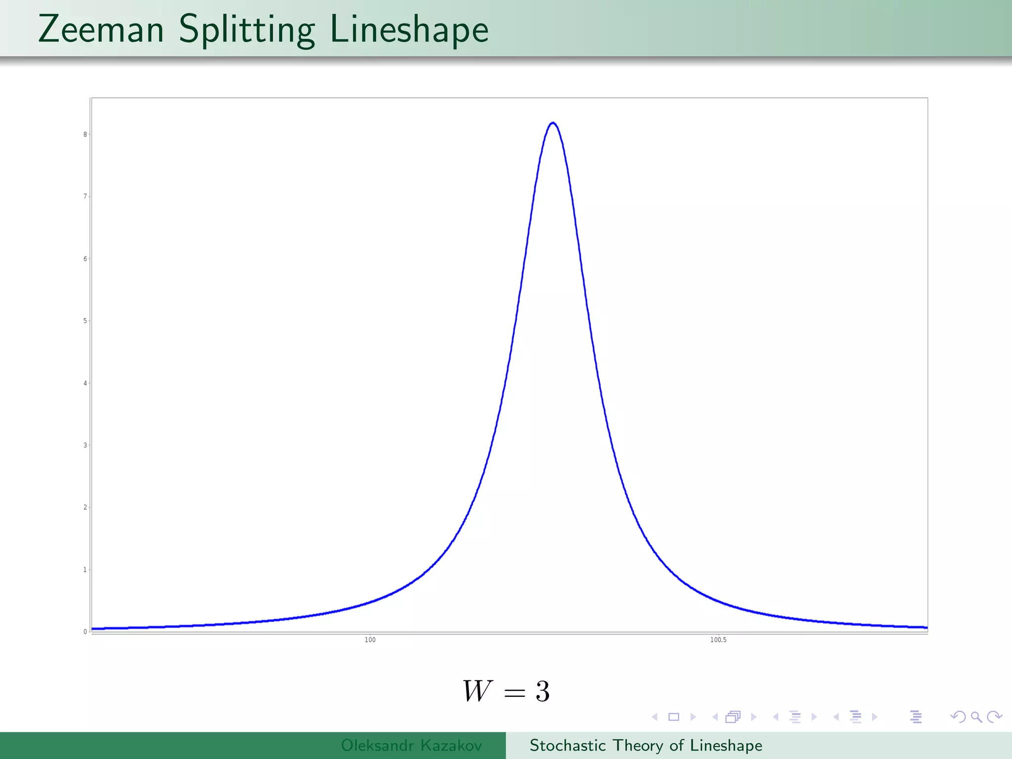
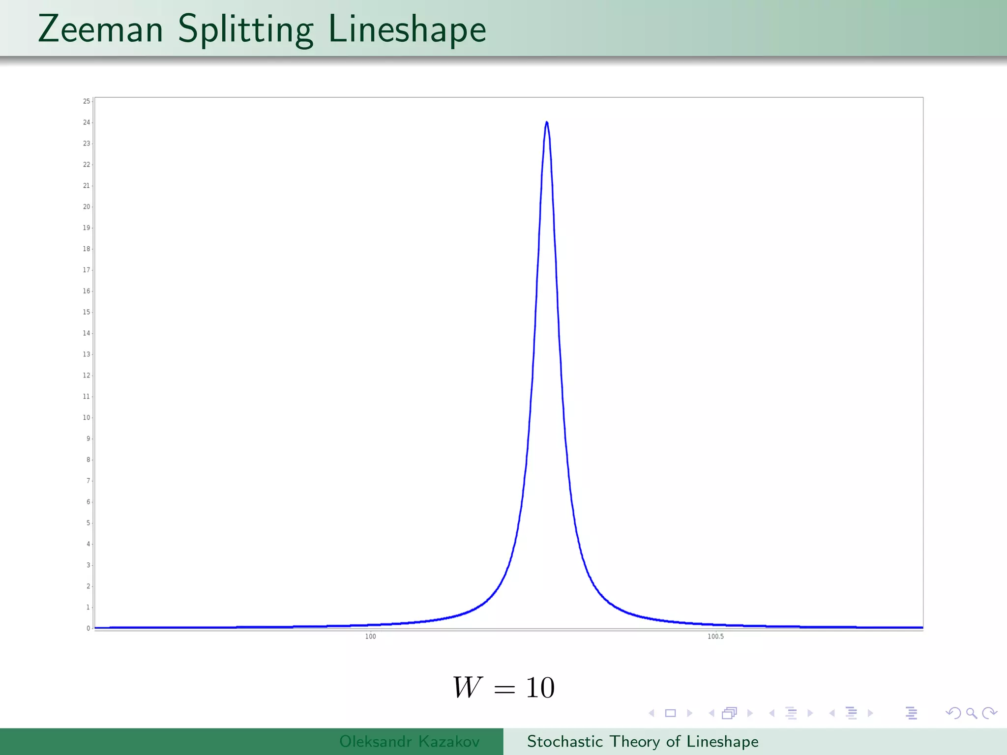
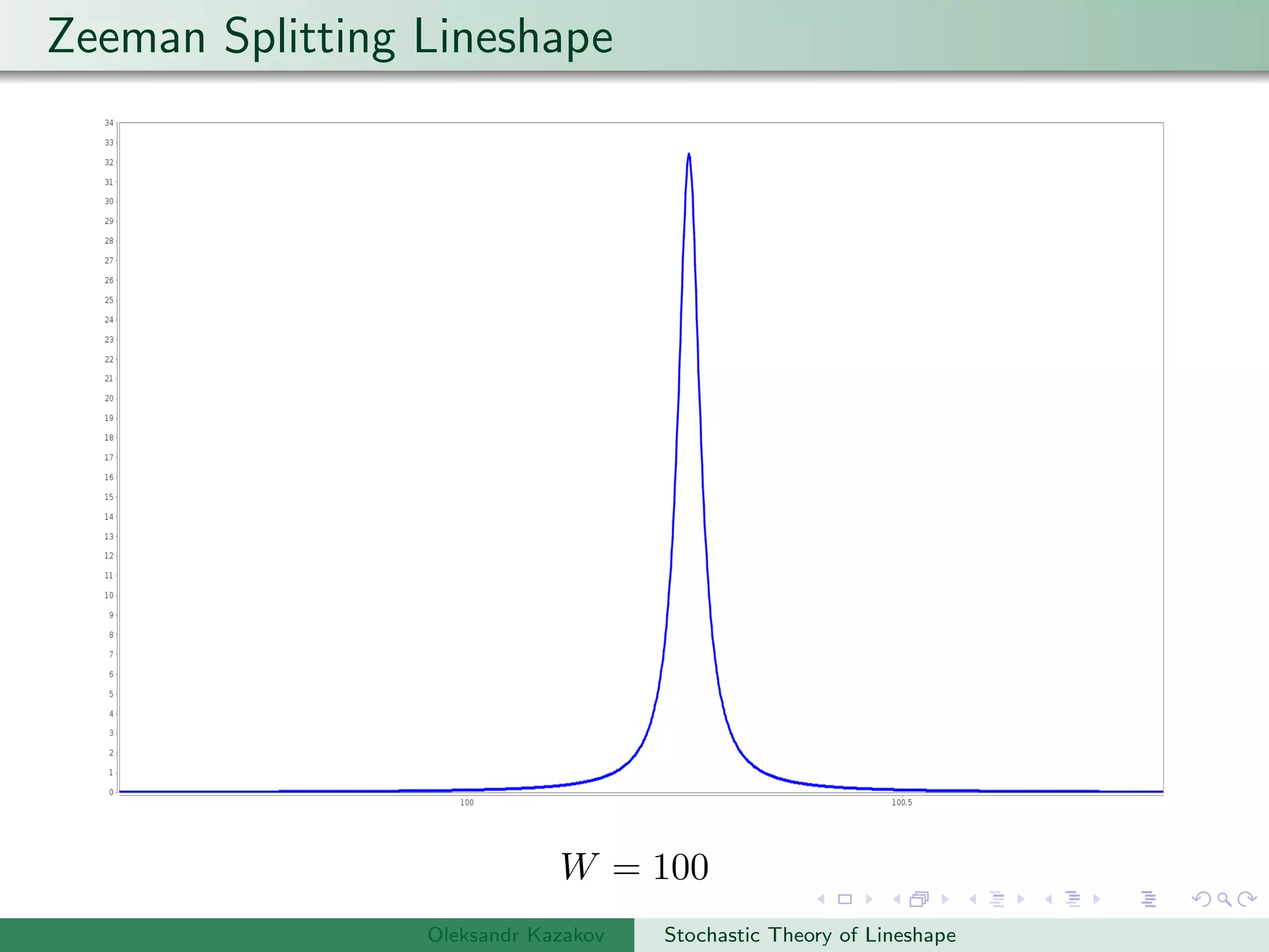
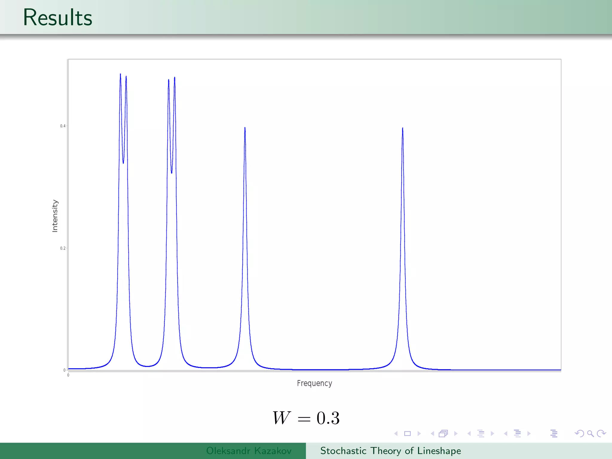
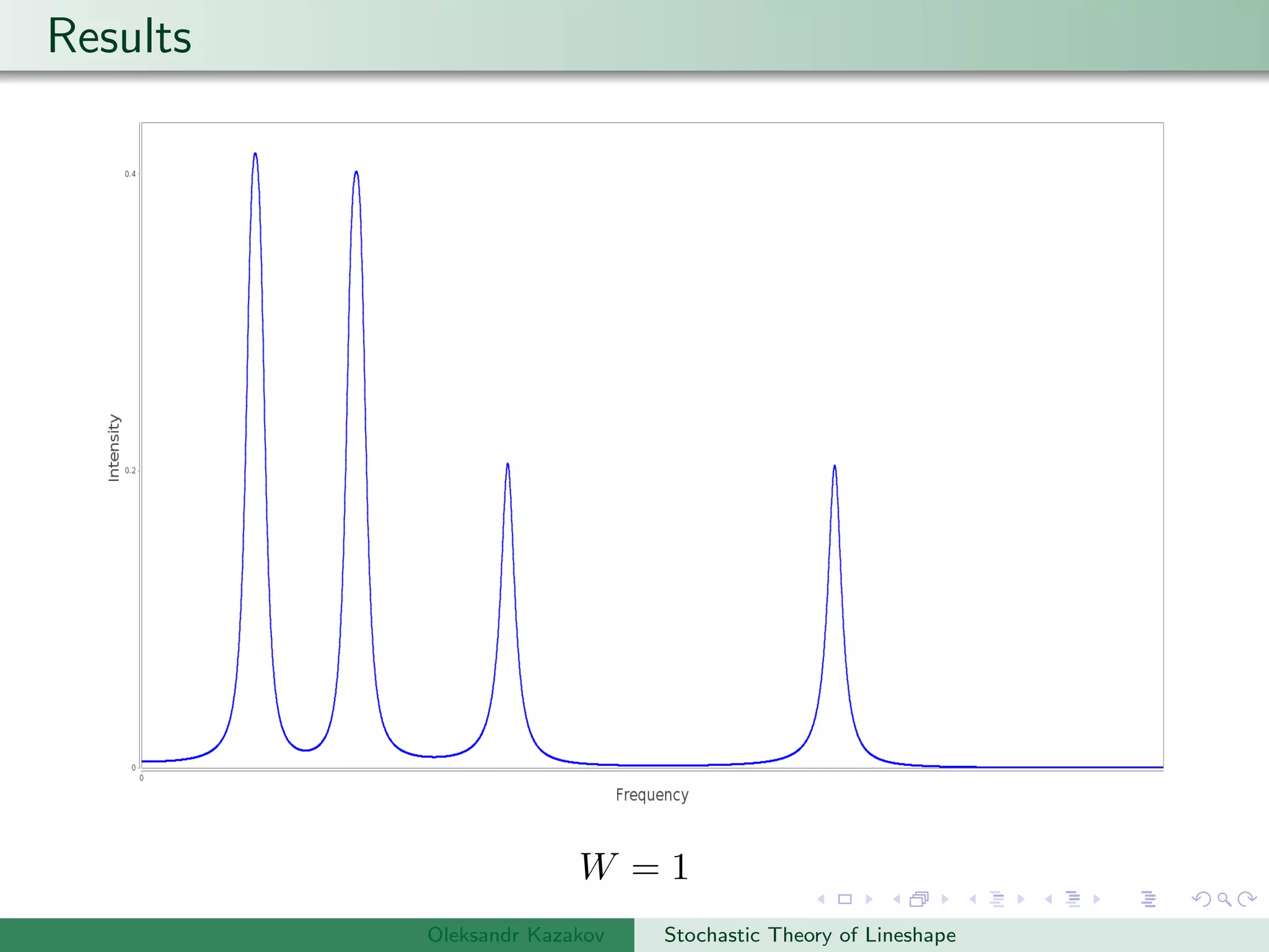
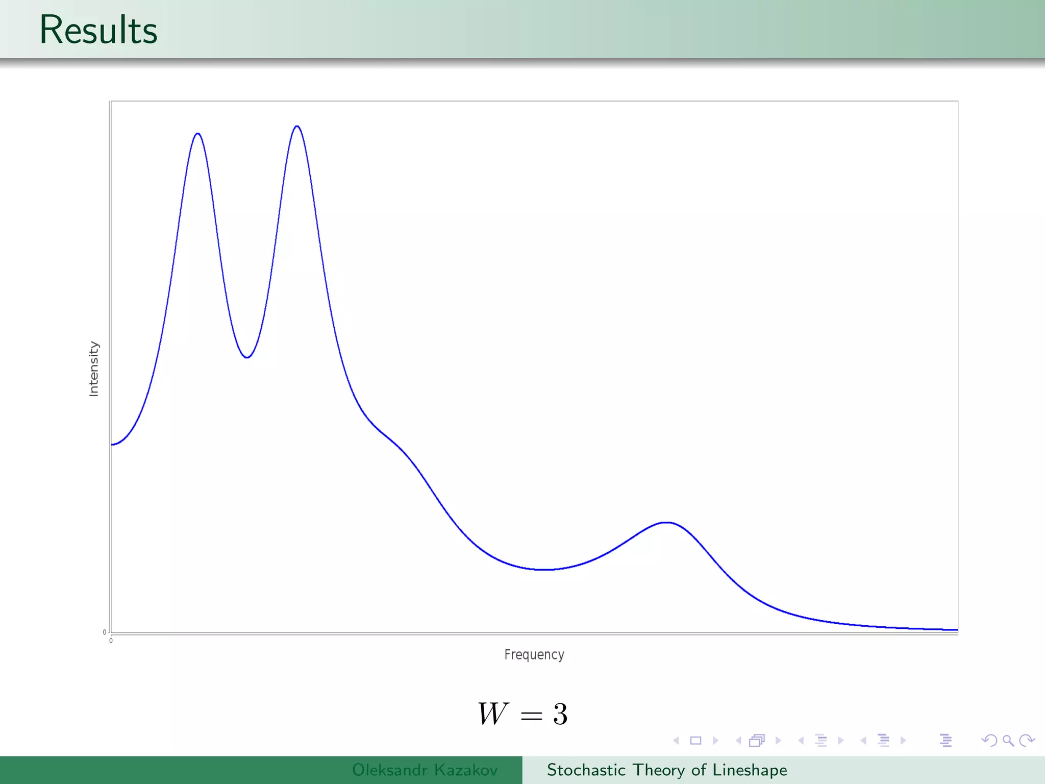
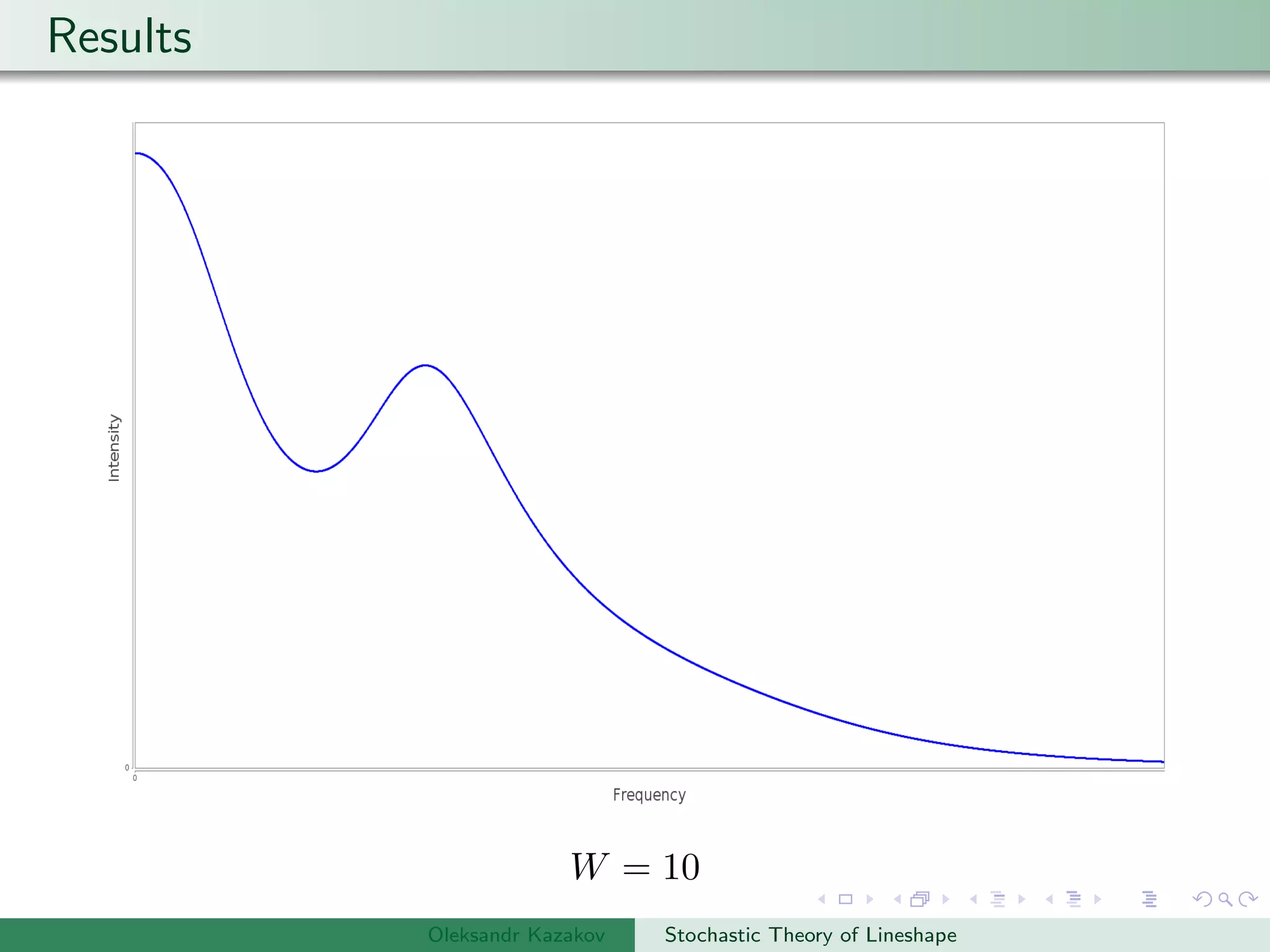
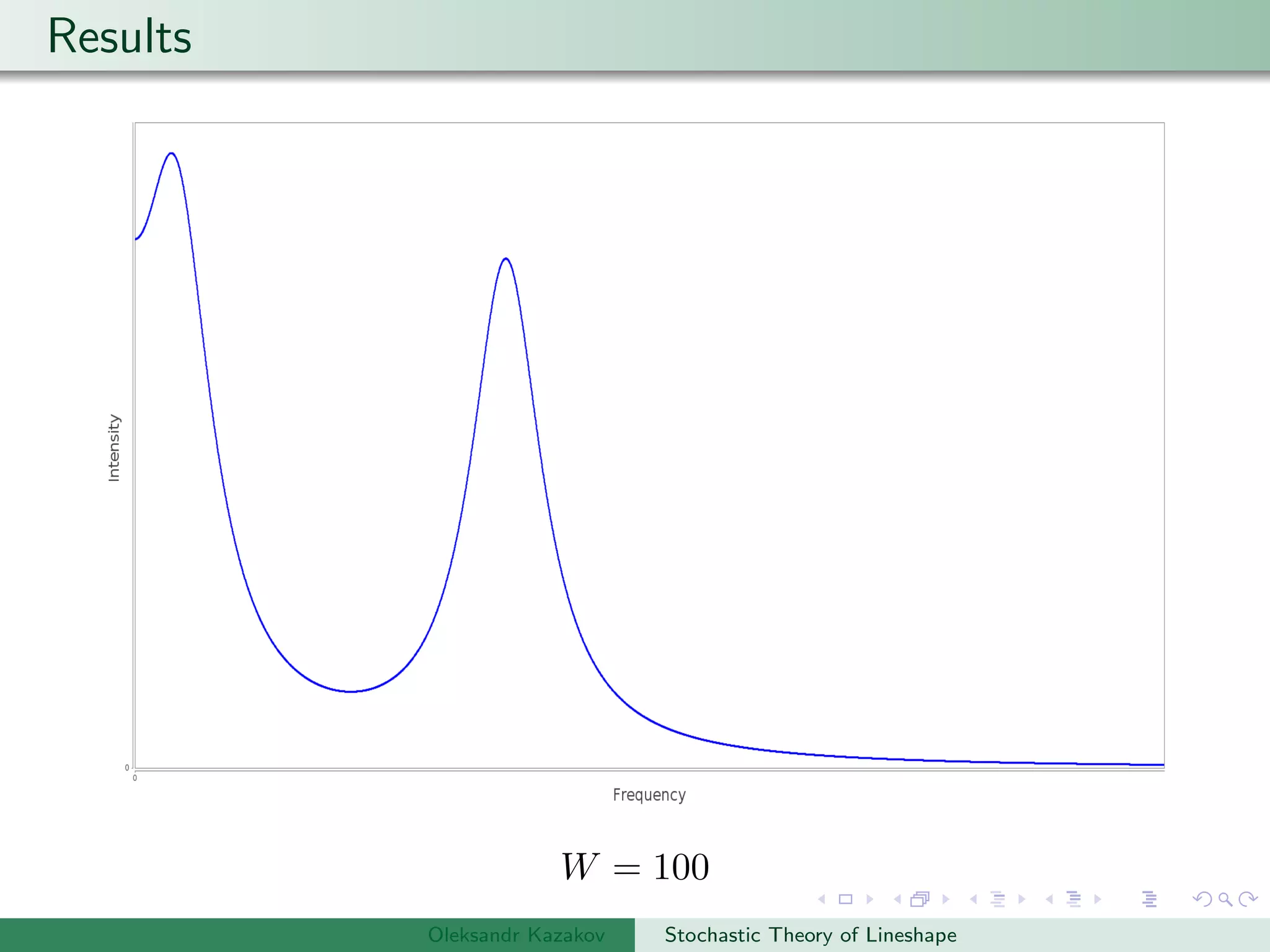
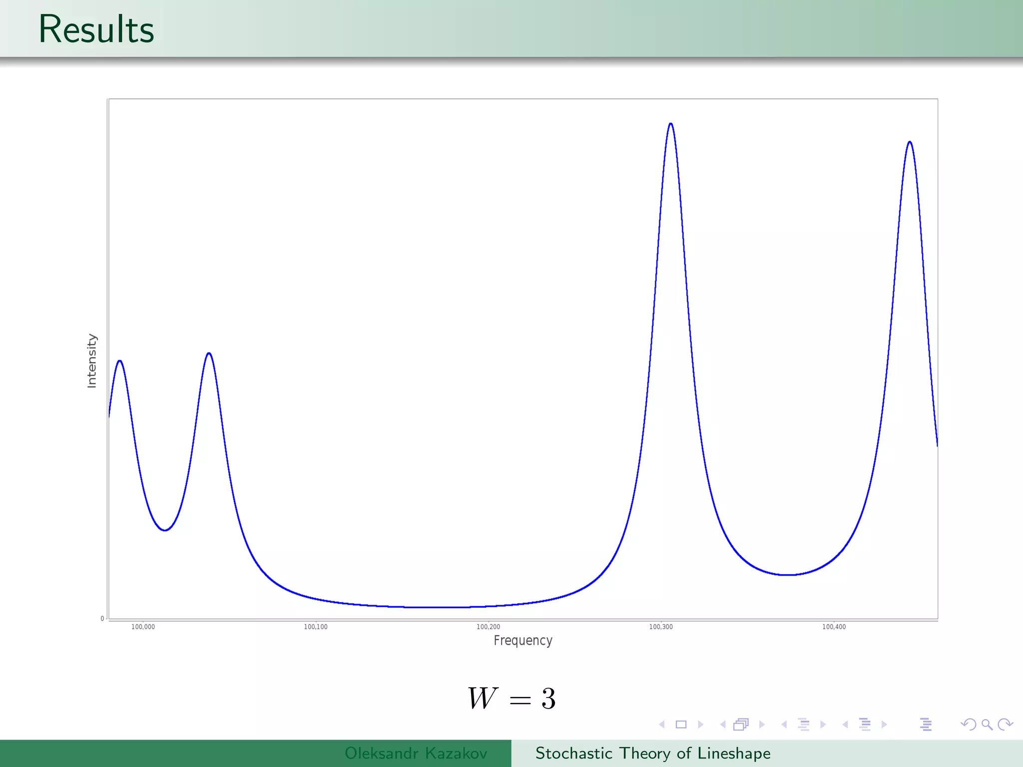
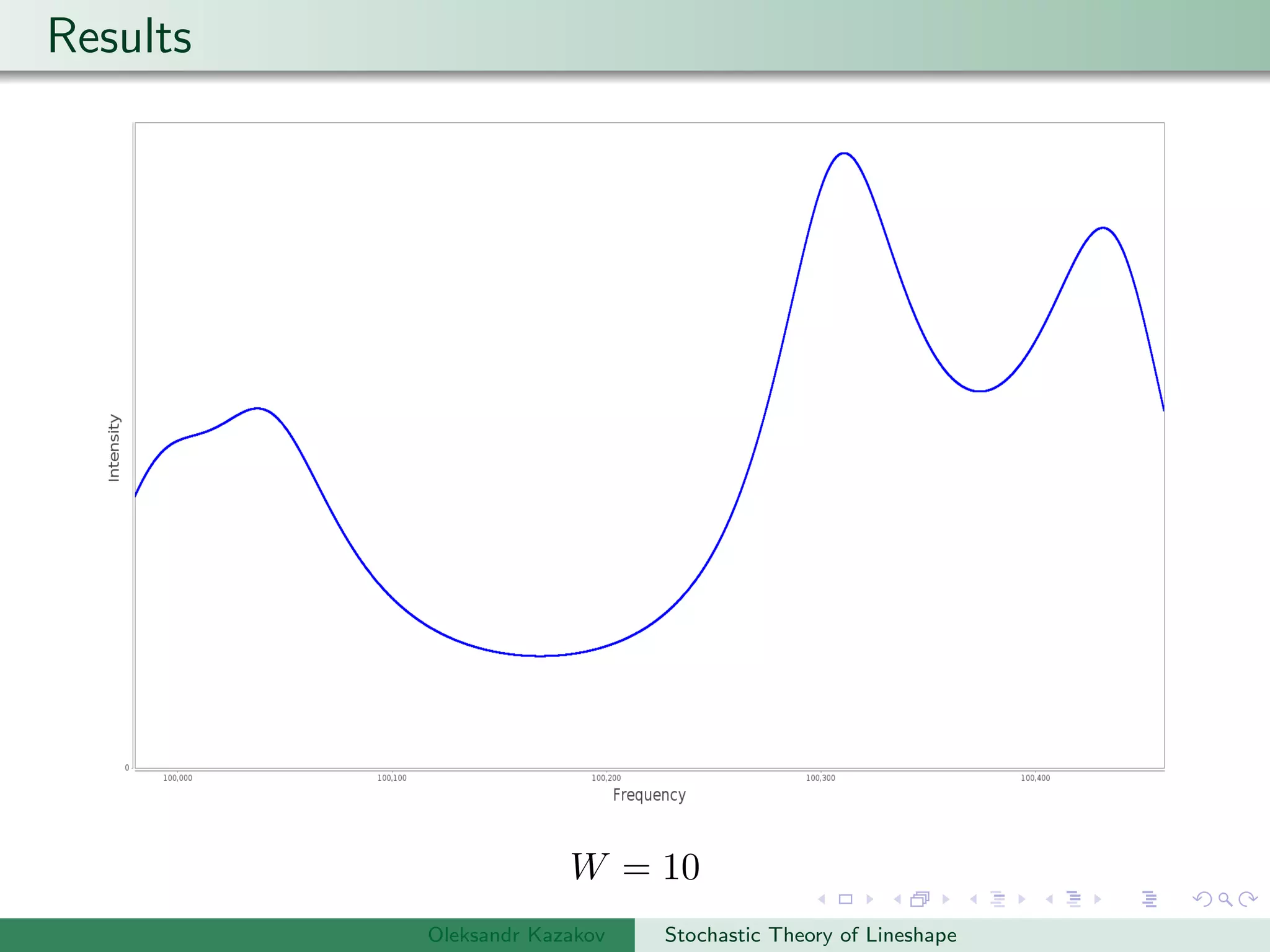
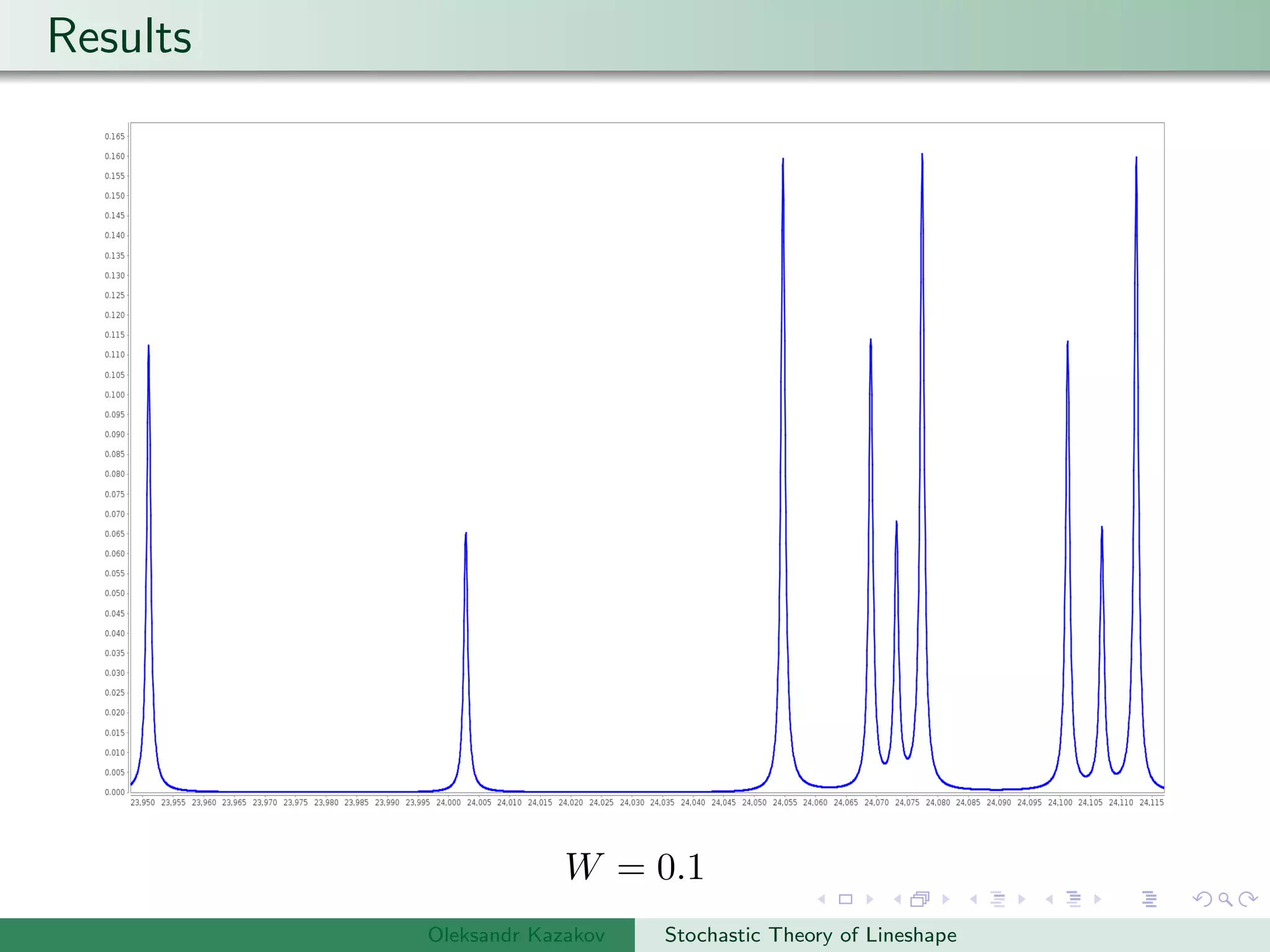
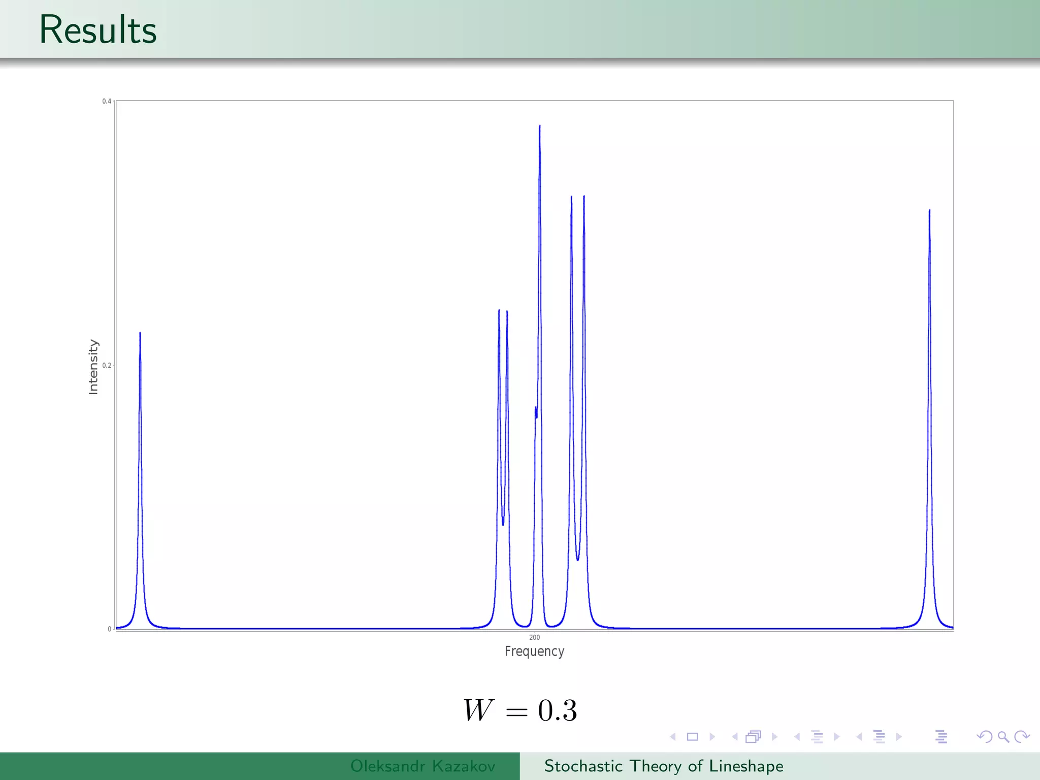
Examples are provided of NMR lineshapes simulated for a spin-1/2 nucleus with different jump rates of a fluctuating magnetic field along the x, y, and z axes.


![Theory Overview
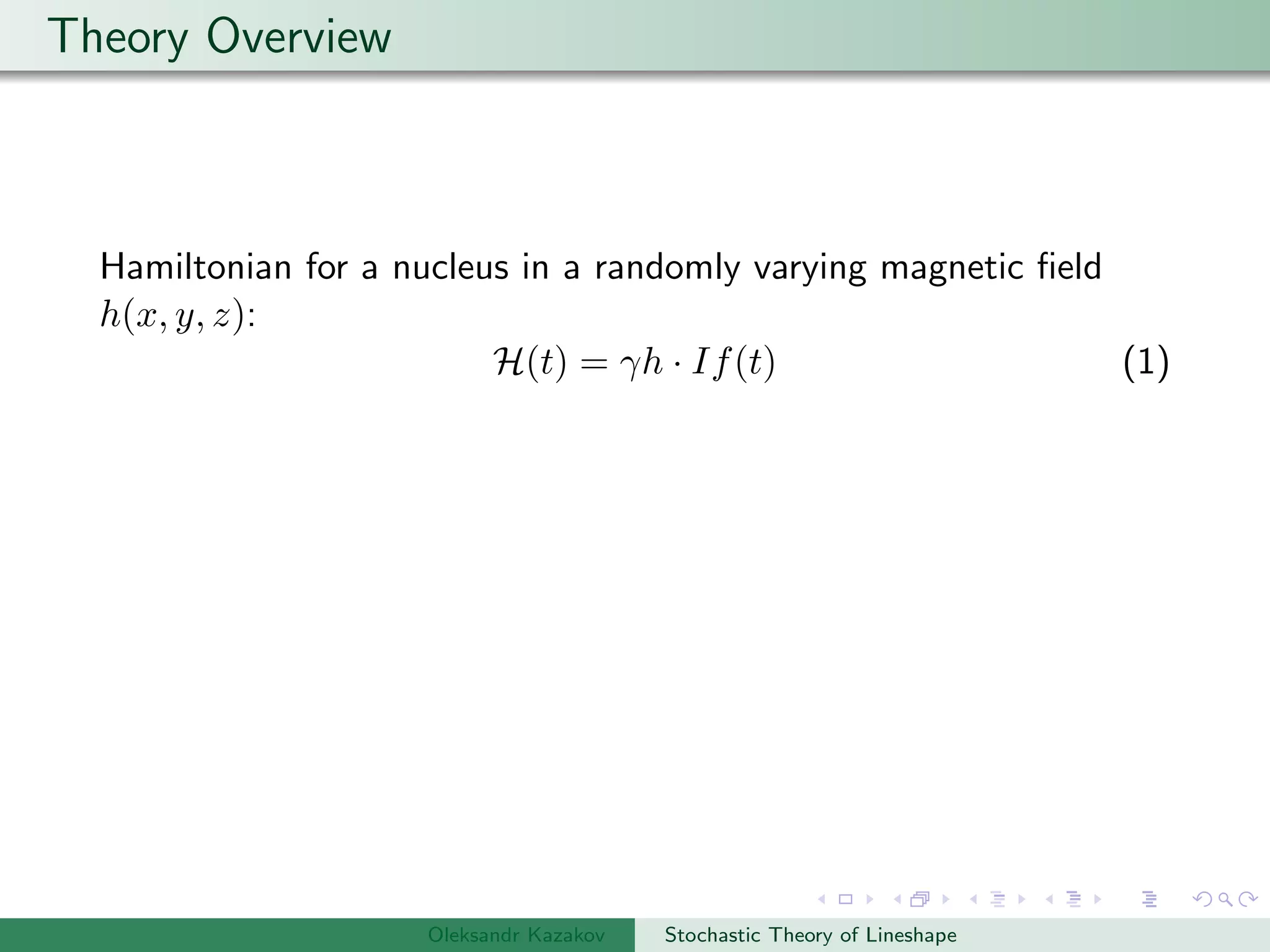
Hamiltonian for a nucleus in a randomly varying magnetic field
h(x, y, z):
H(t) = γh · If(t) (1)
What will happen if we add a fixed magnetic field H0 along
positive x?
H(t) = γH0Iz + γh · If(t) (2)
[H(t), H(t) ] = 0
Oleksandr Kazakov Stochastic Theory of Lineshape](https://image.slidesharecdn.com/bb054024-4d2c-4a62-af38-712fa66765fa-160215160655/75/Oral-Exam-Slides-7-2048.jpg)


![Theory Overview
For easier implementation we can also rewritte as:
P(s) =
2
Γ(2I0 + 1)
H(−)
δm1m0 H(+)
δm0m1
[sδabδm1m1
δm0m0
− (a|W|b)δm0m0
δm1m1
− i(a|F|a)δab[ I0m0|Vj|I0m0 δm0m0
− I1m1|Vj|I1m1 δm1m1
]−1
(9)
Oleksandr Kazakov Stochastic Theory of Lineshape](https://image.slidesharecdn.com/bb054024-4d2c-4a62-af38-712fa66765fa-160215160655/75/Oral-Exam-Slides-14-2048.jpg)
![Problem
Algorithm to generate arrays values and perform where index i and
j for Ai,j are composed of 3 subindices A(m0,m1,a),(m0,m1,b) in a
simplest case having only nuclear spin.
Ai,j = A(m0S,m1S,m0I ,m1I ,a),(m0S,m1S,m0I ,m1I ,b) =
[sδabδm1m1
δm0m0
− (a|W|b)δm0m0
δm1m1
− i(a|F|a)δab[ I0m0|Vj|I0m0 δm0m0
− I1m1|Vj|I1m1 δm1m1
]−1
(10)
It is possible to do assignment of Liouville Matrix by hand up to
size 8 × 8 but what if its size expands to 256 × 256 or
1 · 106 × 1 · 106?
Oleksandr Kazakov Stochastic Theory of Lineshape](https://image.slidesharecdn.com/bb054024-4d2c-4a62-af38-712fa66765fa-160215160655/75/Oral-Exam-Slides-15-2048.jpg)


![Algorithm Development in Stages
Generate 6-D array: A[a][b][m0][m1][m0][m1]
Oleksandr Kazakov Stochastic Theory of Lineshape](https://image.slidesharecdn.com/bb054024-4d2c-4a62-af38-712fa66765fa-160215160655/75/Oral-Exam-Slides-19-2048.jpg)
![Algorithm Development in Stages
Generate 6-D array: A[a][b][m0][m1][m0][m1]
Cast 6-D array into 2-D: A[a][b][m0][m1][m0][m1] → A [i][j]
Oleksandr Kazakov Stochastic Theory of Lineshape](https://image.slidesharecdn.com/bb054024-4d2c-4a62-af38-712fa66765fa-160215160655/75/Oral-Exam-Slides-20-2048.jpg)
![Algorithm Development in Stages
Generate 6-D array: A[a][b][m0][m1][m0][m1]
Cast 6-D array into 2-D: A[a][b][m0][m1][m0][m1] → A [i][j]
Perform 2-D array inversion: A [i][j] = A [i][j]−1
Oleksandr Kazakov Stochastic Theory of Lineshape](https://image.slidesharecdn.com/bb054024-4d2c-4a62-af38-712fa66765fa-160215160655/75/Oral-Exam-Slides-21-2048.jpg)
![Algorithm Development in Stages
Generate 6-D array: A[a][b][m0][m1][m0][m1]
Cast 6-D array into 2-D: A[a][b][m0][m1][m0][m1] → A [i][j]
Perform 2-D array inversion: A [i][j] = A [i][j]−1
Cast 2-D array back into 6-D array:
A [i][j] → A[a][b][m0][m1][m0][m1]
Oleksandr Kazakov Stochastic Theory of Lineshape](https://image.slidesharecdn.com/bb054024-4d2c-4a62-af38-712fa66765fa-160215160655/75/Oral-Exam-Slides-22-2048.jpg)
![Algorithm Development in Stages
Generate 6-D array: A[a][b][m0][m1][m0][m1]
Cast 6-D array into 2-D: A[a][b][m0][m1][m0][m1] → A [i][j]
Perform 2-D array inversion: A [i][j] = A [i][j]−1
Cast 2-D array back into 6-D array:
A [i][j] → A[a][b][m0][m1][m0][m1]
Go back to the equation 6 and do the summation.
Oleksandr Kazakov Stochastic Theory of Lineshape](https://image.slidesharecdn.com/bb054024-4d2c-4a62-af38-712fa66765fa-160215160655/75/Oral-Exam-Slides-23-2048.jpg)
![Algorithm Development in Stages
Generate 6-D array: A[a][b][m0][m1][m0][m1]
Cast 6-D array into 2-D: A[a][b][m0][m1][m0][m1] → A [i][j]
Perform 2-D array inversion: A [i][j] = A [i][j]−1
Cast 2-D array back into 6-D array:
A [i][j] → A[a][b][m0][m1][m0][m1]
Go back to the equation 6 and do the summation.
Plot the results.
Oleksandr Kazakov Stochastic Theory of Lineshape](https://image.slidesharecdn.com/bb054024-4d2c-4a62-af38-712fa66765fa-160215160655/75/Oral-Exam-Slides-24-2048.jpg)
![Encoding Table Example
A simple example of encription of 6 different combinations between
3 indecies that are used to cast back 6-D array from
2-D(A[a][:][m0][m1][:][:] → A [i][:]).
a, m0, m1 Output Count
1, 1/2, 1/2 → 000 1
1, −1/2, 1/2 → 010 2
1, 1/2, −1/2 → 001 3
2, 1/2, 1/2 → 100 4
2, 1/2, 1/2 → 101 5
2, −1/2, −1/2 → 111 6
Oleksandr Kazakov Stochastic Theory of Lineshape](https://image.slidesharecdn.com/bb054024-4d2c-4a62-af38-712fa66765fa-160215160655/75/Oral-Exam-Slides-25-2048.jpg)
![Code Sample
Java Method to store reference for the elements of 6-D array after
converting into 2-D array. Elements being converted and saved
into string format.
public static String[] genind(int m_0,int m_1, int a1 ){
int x=1;
String Y[] = new String[max];
for(int k=0;k<m_0;k++){
for(int l=0;l<m_1;l++){
for(int a=0;a<a1;a++){
Y[x-1]=String.format("%03d",a+10*k+100*l);
x++;
}
}
}
return Y;
} Oleksandr Kazakov Stochastic Theory of Lineshape](https://image.slidesharecdn.com/bb054024-4d2c-4a62-af38-712fa66765fa-160215160655/75/Oral-Exam-Slides-26-2048.jpg)
![Code Sample
Casting 6-D array into 2-D:
for(int k=0; k<m_0;k++){
for(int l=0; l<m_1; l++){
for(int m=0; m<m_01; m++){
for(int n=0;n<m_11; n++){
for(int a=0; a<a1; a++){
for(int b=0; b<b1;b++){
tr[index(k,l,a,Y)][index(m,n,b,Y)]=matrix[a][b][k][l][m][n];
}
}
}
}
}
}
return tr;
}
Oleksandr Kazakov Stochastic Theory of Lineshape](https://image.slidesharecdn.com/bb054024-4d2c-4a62-af38-712fa66765fa-160215160655/75/Oral-Exam-Slides-27-2048.jpg)
![Code Sample
Converting from 2-D array back to 6-D array:
public static Object[][][][][][] matrixturn(Complex
tr[][], String Y[]){
for(int k=0; k<max;k++){
for(int l=0; l<max; l++){
hn[a1indback(k,Y)][b1indback(l,Y)][m0indback(k,Y)]...
[m1indback(k,Y)][m01indback(l,Y)][m11indback(l,Y)]=tr[k][l];
}
}
return hamatrixnew;
}
Oleksandr Kazakov Stochastic Theory of Lineshape](https://image.slidesharecdn.com/bb054024-4d2c-4a62-af38-712fa66765fa-160215160655/75/Oral-Exam-Slides-28-2048.jpg)
![Code Sample
Method for the extraction of element reference in 2-D array to that
in 6-D:
public static int m0indexback( int k, String Y[]){
int m0=0;
int f=Integer.parseInt(Y[k]);
m0=(int) Math.floor((f/100));
return m0;
}
public static int m1indexback( int k,String Y[]){
int m1=0;
int ff=Integer.parseInt(Y[k]);
m1=(int) Math.floor((ff-Math.floor(ff/100)*100)/10);
return m1;
}
Oleksandr Kazakov Stochastic Theory of Lineshape](https://image.slidesharecdn.com/bb054024-4d2c-4a62-af38-712fa66765fa-160215160655/75/Oral-Exam-Slides-29-2048.jpg)
![Code Sample
Method for the extraction of element reference in 2-D array to that
in 6-D to perform summation:
public static int a1indexback(int k,String Y[]){
int fff=Integer.parseInt(Y[k]);
int a1=0;
a1= (int) (Math.floor(fff-Math.floor(fff/100)*100)-...
Math.floor((fff-Math.floor(fff/100)*100)/10)*10);
return a1;
}
Oleksandr Kazakov Stochastic Theory of Lineshape](https://image.slidesharecdn.com/bb054024-4d2c-4a62-af38-712fa66765fa-160215160655/75/Oral-Exam-Slides-30-2048.jpg)


±2(g) = −
1
2
βe(gxx − gyy) A
[2](P)
±2(g) = 0
F
[2](P)
±1(g) = 0 A
[2](P)
±1(g) = 0
F
[2](P)
0(g) = −
2
3
βe(gzz −
1
2
(gxx + gyy) A
[2](P)
0(g) = −
2
3
SzHz
F
[0](P)
0(g) =
1
√
3
(gxx + gyy + gzz A
[0](P)
0(g) =
1
√
3
)
Oleksandr Kazakov Stochastic Theory of Lineshape](https://image.slidesharecdn.com/bb054024-4d2c-4a62-af38-712fa66765fa-160215160655/75/Oral-Exam-Slides-57-2048.jpg)

m(g) = (Dl
m,2(ΩL→P ) + Dl
m,−2(ΩL→P ))∗F
[2](P)
2(g) + (Dl
m,0(ΩL→P ))∗F
[2](P)
0(g)
F tensor components should satisfy identity:
(F
[l]
q )∗ = (−1)2+qF
[l]
−q
Oleksandr Kazakov Stochastic Theory of Lineshape](https://image.slidesharecdn.com/bb054024-4d2c-4a62-af38-712fa66765fa-160215160655/75/Oral-Exam-Slides-58-2048.jpg)
![Coordinate Frames Transformation(Explicit)
F
[2],(L)
1(g) = −(F
[2],(L)
−1(g) )∗
= −e−iα
([sin(β)cos(β)cos(2γ) − isin(β)sin(2γ)]F
2(P)
2(g) −
3
2
sin(β)cos(β)F
2(P)
0(g) )
F
[2],(L)
0(g) =
3
2
sin2
(β)cos(2γ)F
2(P)
2(g) +
1
2
(3cos2
(β) − 1)F
2(P)
0(g)
F
[2],(L)
2(g) = (F
[2],(L)
−2(g) )∗
= ei2α
([
1 + cos2(β)
2
cos(2γ) + icos(β)sin(2γ)]F
2(P)
2(g) +
3
8
sin2
(β)F
2(P)
0(g) )
Oleksandr Kazakov Stochastic Theory of Lineshape](https://image.slidesharecdn.com/bb054024-4d2c-4a62-af38-712fa66765fa-160215160655/75/Oral-Exam-Slides-59-2048.jpg)
![Zeeman Splitting
Now we all set to construct Hamiltonian where all quantities are
evaluated in the lab frame:
Hzm = A
[2]
0 F
[2]
0 + A
[0]
0 F
[0]
0
Oleksandr Kazakov Stochastic Theory of Lineshape](https://image.slidesharecdn.com/bb054024-4d2c-4a62-af38-712fa66765fa-160215160655/75/Oral-Exam-Slides-60-2048.jpg)


±2(hf) = −
1
2
βe(Axx − Ayy) A
[2](P)
±2(hf) = −
1
2
S±I±
F
[2](P)
±1(hf) = 0 A
[2](P)
±1(hf) = ±
1
2
(S±Iz + SzI±)
F
[2](P)
0(hf) = −
2
3
βe(Azz −
1
2
(Axx + Ayy)) A
[2](P)
0(hf) = −
2
3
SzIz −
1
4
(S+I− + S−I+)
F
[0](P)
0(hf) =
1
√
3
(Axx + Ayy + Azz) A
[0](P)
0(hf) =
1
√
3
SzIz −
1
4
(S+I− + S−I+)
Oleksandr Kazakov Stochastic Theory of Lineshape](https://image.slidesharecdn.com/bb054024-4d2c-4a62-af38-712fa66765fa-160215160655/75/Oral-Exam-Slides-69-2048.jpg)
![In the same manner as Zeeman Hamiltonian we can rewritte:
Hhf = A
[2]
0 F
[2]
0 + A
[0]
0 F
[0]
0 + A
[2]
1 (F
[2]
1 )∗
+ A
[2]
−1F
[2]
1
so generalizing:
Hres = Hzm + Hhf
Oleksandr Kazakov Stochastic Theory of Lineshape](https://image.slidesharecdn.com/bb054024-4d2c-4a62-af38-712fa66765fa-160215160655/75/Oral-Exam-Slides-70-2048.jpg)


![11.[1 7]fuzzy join prime semi l-ideals](https://cdn.slidesharecdn.com/ss_thumbnails/11-1-7fuzzyjoinprimesemil-ideals-120512235333-phpapp02-thumbnail.jpg?width=640&height=640&fit=bounds)


