Download free for 30 days
Sign in
Upload
Language (EN)
Support
Business
Mobile
Social Media
Marketing
Technology
Art & Photos
Career
Design
Education
Presentations & Public Speaking
Government & Nonprofit
Healthcare
Internet
Law
Leadership & Management
Automotive
Engineering
Software
Recruiting & HR
Retail
Sales
Services
Science
Small Business & Entrepreneurship
Food
Environment
Economy & Finance
Data & Analytics
Investor Relations
Sports
Spiritual
News & Politics
Travel
Self Improvement
Real Estate
Entertainment & Humor
Health & Medicine
Devices & Hardware
Lifestyle
Change Language
Language
English
Español
Português
Français
Deutsche
Cancel
Save
EN
Uploaded by
ssuserbad8d3
4 views
Oracle Operational Timing Data for performance tuning
Oracle AWR Data
Technology
◦
Read more
0
Save
Share
Embed
Embed presentation
Download
Download to read offline
1
/ 21
2
/ 21
3
/ 21
4
/ 21
5
/ 21
6
/ 21
7
/ 21
8
/ 21
9
/ 21
10
/ 21
11
/ 21
12
/ 21
13
/ 21
14
/ 21
15
/ 21
16
/ 21
17
/ 21
18
/ 21
19
/ 21
20
/ 21
21
/ 21
More Related Content
PDF
553: Oracle Database Performance: Are Database Users Telling Me The Truth?
by
Alfredo Krieg
PDF
Oracle database performance are database users telling me the truth
by
Alfredo Krieg
PDF
Oracle database performance diagnostics - before your begin
by
Hemant K Chitale
PDF
Yapp methodology anjo-kolk
by
Toon Koppelaars
DOC
Early watch report
by
cecileekove
PDF
Crating a Robust Performance Strategy
by
Guatemala User Group
PDF
Knowledge is Power: Visualizing JIRA's Performance Data
by
Atlassian
PDF
How to find what is making your Oracle database slow
by
SolarWinds
553: Oracle Database Performance: Are Database Users Telling Me The Truth?
by
Alfredo Krieg
Oracle database performance are database users telling me the truth
by
Alfredo Krieg
Oracle database performance diagnostics - before your begin
by
Hemant K Chitale
Yapp methodology anjo-kolk
by
Toon Koppelaars
Early watch report
by
cecileekove
Crating a Robust Performance Strategy
by
Guatemala User Group
Knowledge is Power: Visualizing JIRA's Performance Data
by
Atlassian
How to find what is making your Oracle database slow
by
SolarWinds
Similar to Oracle Operational Timing Data for performance tuning
PPTX
Training - What is Performance ?
by
Betclic Everest Group Tech Team
PDF
What are you waiting for
by
Jason Strate
PDF
“Performance” - Dallas Oracle Users Group 2019-01-29 presentation
by
Cary Millsap
PDF
DB Time, Average Active Sessions, and ASH Math - Oracle performance fundamentals
by
John Beresniewicz
PPTX
Oracle database performance tuning
by
Yogiji Creations
PDF
Donatone_Grid Performance(2)11111111.pdg
by
cookie1969
PDF
Database & Technology 1 _ Craig Shallahamer _ Unit of work time based perform...
by
InSync2011
PDF
pdf-download-db-time-based-oracle-performance-tuning-theory-and.pdf
by
cookie1969
PPTX
Master tuning
by
Thomas Kejser
PDF
10 tips-for-optimizing-sql-server-performance-white-paper-22127
by
Kaizenlogcom
PDF
Awr + 12c performance tuning
by
AiougVizagChapter
PPTX
Metric Abuse: Frequently Misused Metrics in Oracle
by
Steve Karam
PDF
Database & Technology 1 _ Craig Shallahamer _ SQL Elapsed Time Analhysis.pdf
by
InSync2011
PDF
Calculating SQL Runtime Using Raw ASH Data.pdf
by
Yuan Yao
PDF
AWR & ASH Analysis
by
aioughydchapter
PDF
Presentation maximizing database performance performance tuning with db time
by
xKinAnx
PPTX
Operation Analytics and Investigating Metric Spike - Report.pptx
by
Arnab Bhattacharya
PDF
Oracle database performance tuning
by
Abishek V S
PPTX
Performance Forensics - Understanding Application Performance
by
Alois Reitbauer
PPT
Les 14 perf_db
by
Femi Adeyemi
Training - What is Performance ?
by
Betclic Everest Group Tech Team
What are you waiting for
by
Jason Strate
“Performance” - Dallas Oracle Users Group 2019-01-29 presentation
by
Cary Millsap
DB Time, Average Active Sessions, and ASH Math - Oracle performance fundamentals
by
John Beresniewicz
Oracle database performance tuning
by
Yogiji Creations
Donatone_Grid Performance(2)11111111.pdg
by
cookie1969
Database & Technology 1 _ Craig Shallahamer _ Unit of work time based perform...
by
InSync2011
pdf-download-db-time-based-oracle-performance-tuning-theory-and.pdf
by
cookie1969
Master tuning
by
Thomas Kejser
10 tips-for-optimizing-sql-server-performance-white-paper-22127
by
Kaizenlogcom
Awr + 12c performance tuning
by
AiougVizagChapter
Metric Abuse: Frequently Misused Metrics in Oracle
by
Steve Karam
Database & Technology 1 _ Craig Shallahamer _ SQL Elapsed Time Analhysis.pdf
by
InSync2011
Calculating SQL Runtime Using Raw ASH Data.pdf
by
Yuan Yao
AWR & ASH Analysis
by
aioughydchapter
Presentation maximizing database performance performance tuning with db time
by
xKinAnx
Operation Analytics and Investigating Metric Spike - Report.pptx
by
Arnab Bhattacharya
Oracle database performance tuning
by
Abishek V S
Performance Forensics - Understanding Application Performance
by
Alois Reitbauer
Les 14 perf_db
by
Femi Adeyemi
Recently uploaded
PDF
Transcript: Escape from the Forbidden Zone: Smuggling green and inclusive tec...
by
BookNet Canada
PDF
Constraint Collapse and Fidelity Decay in Scaled Language Models
by
Semantic Fidelity Lab | A. Jacobs
PDF
NTG -Company Profile_Software_Vendor_Company_in_MENA
by
Mustafa Kuğu
PDF
HOW TO OVERCOME THE THREATS OF ARTIFICIAL INTELLIGENCE AGAINST HUMANITY.pdf
by
Faga1939
PDF
February 2026 Patch Tuesday hosted by Chris Goettl and Todd Schell
by
Ivanti
PPTX
Tech Trends 2026: AI Agents, Quantum Computing, Robotics & Cybersecurity
by
ridwansassman
PDF
Explaining specific examples of purpose-specific BOM
by
akipii ogaoga
PDF
Session 1/5: Enhancing Automation with Screenplay & Business Rules
by
suhanisingh58689
PPTX
CTO Strategy OS 2026: The Tech, AI & Cloud Playbook Boards Want
by
ridwansassman
PDF
Chapter 5 Security Mechanisms iin computer security.pdf
by
Getnet Tigabie Askale -(GM)
PDF
Effortless Distributed Systems with Aspire.pdf
by
Particular Software
PDF
Automated Governance for FME Flow: Smarter Admin at Scale
by
Safe Software
PDF
TrustArc Webinar - From Trends to Action: Fitting AI Governance into Privacy Ops
by
TrustArc
PDF
GDG Cloud Southlake #49: Pradeep R Kumar: Implications of Agentic AI for Iden...
by
James Anderson
PDF
20260212 Security-JAWS activity results for 2025 and activity goals for 2026
by
Typhon 666
PPTX
Do You Control the AI, or Does the AI Control You?
by
medhateltoukhy
PDF
GenerationAI_Paris_2025_Architecting_Intelligence.pdf
by
apidays
PDF
apidays Paris 2025 | Zero Trust By Design
by
apidays
PDF
How does MES(Manufacturing Execution System) work?
by
akipii ogaoga
PDF
Oracle Cloud Infrastructure 2025 Architect Professional (1Z0-1127-25) Master ...
by
ExamCert App
Transcript: Escape from the Forbidden Zone: Smuggling green and inclusive tec...
by
BookNet Canada
Constraint Collapse and Fidelity Decay in Scaled Language Models
by
Semantic Fidelity Lab | A. Jacobs
NTG -Company Profile_Software_Vendor_Company_in_MENA
by
Mustafa Kuğu
HOW TO OVERCOME THE THREATS OF ARTIFICIAL INTELLIGENCE AGAINST HUMANITY.pdf
by
Faga1939
February 2026 Patch Tuesday hosted by Chris Goettl and Todd Schell
by
Ivanti
Tech Trends 2026: AI Agents, Quantum Computing, Robotics & Cybersecurity
by
ridwansassman
Explaining specific examples of purpose-specific BOM
by
akipii ogaoga
Session 1/5: Enhancing Automation with Screenplay & Business Rules
by
suhanisingh58689
CTO Strategy OS 2026: The Tech, AI & Cloud Playbook Boards Want
by
ridwansassman
Chapter 5 Security Mechanisms iin computer security.pdf
by
Getnet Tigabie Askale -(GM)
Effortless Distributed Systems with Aspire.pdf
by
Particular Software
Automated Governance for FME Flow: Smarter Admin at Scale
by
Safe Software
TrustArc Webinar - From Trends to Action: Fitting AI Governance into Privacy Ops
by
TrustArc
GDG Cloud Southlake #49: Pradeep R Kumar: Implications of Agentic AI for Iden...
by
James Anderson
20260212 Security-JAWS activity results for 2025 and activity goals for 2026
by
Typhon 666
Do You Control the AI, or Does the AI Control You?
by
medhateltoukhy
GenerationAI_Paris_2025_Architecting_Intelligence.pdf
by
apidays
apidays Paris 2025 | Zero Trust By Design
by
apidays
How does MES(Manufacturing Execution System) work?
by
akipii ogaoga
Oracle Cloud Infrastructure 2025 Architect Professional (1Z0-1127-25) Master ...
by
ExamCert App
Oracle Operational Timing Data for performance tuning
1.
Copyright © 2003
by Hotsos Enterprises, Ltd. All rights reserved. 1 Oracle Operational Timing Data Cary Millsap Hotsos Enterprises, Ltd. Introduction In 1992, Oracle Corporation published release 7.0.12 of the Oracle database kernel. This was the first release of the database that made public a new feature that many people call the Oracle wait interface. Only since the year 2000 has this wait interface begun to gather real momentum among database administrators in the mass market. Even today, fully eleven years after its introduction, Oracle’s operational timing data is severely underutilized even by many of the individuals who led the way to our use of the wait interface. This paper lays the groundwork for correcting the problem. Important Advances I’ll introduce the subject of Oracle operational timing data by describing what I believe to be the three most important advances that I’ve witnessed in the part of my career devoted to working with Oracle products. Curiously, while these advances are certainly new to most professionals who work with Oracle products, none of these advances is really “new.” Each is used extensively by optimization analysts in non-Oracle fields. User Action Focus The first important advance in Oracle optimization technology follows from a simple mathematical observation: You can’t extrapolate detail from an aggregate.
2.
Copyright © 2003
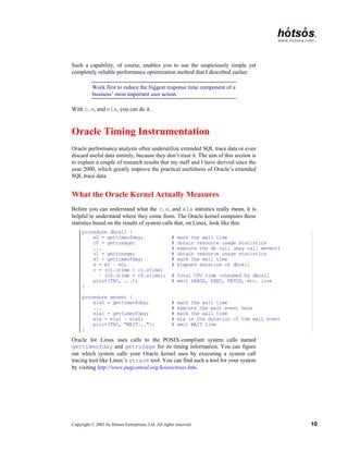
by Hotsos Enterprises, Ltd. All rights reserved. 2 Here’s a puzzle to demonstrate my point. Imagine that I told you that a collection of 1,000 rocks contains 999 grey rocks and one special rock that’s painted bright red. The collection weighs 1,000 pounds. Now, answer the following question, “How much does the red rock weigh?” If your answer is, “I know that the red rock weighs 1 pound,” then you’ve simply told a lie. You don’t know that; with the information you’ve been given, you can’t. If your answer is, “I assume that the red rock weighs 1 pound,” then you’re asking for big trouble. Such an assumption puts you at grave risk of forming conclusions that are stunningly incorrect. The correct answer is that the red rock can weigh virtually any amount between zero and 1,000 pounds. The only thing limiting the low end of the weight is the definition of how many atoms must be present in order for a thing to be called a rock. Once we define how small a rock can be, then we’ve defined the high end of our answer. It is 1,000 pounds minus the weight of 999 of the smallest possible rocks. The red rock can weigh literally anything between those two values. Answering with any more precision is wrong unless you happen to be very lucky. But being very lucky at games like this is a skill that can be neither learned nor taught, nor repeated with acceptable reliability. This is one reason why Oracle analysts find it so frustrating to diagnose performance problems armed only with system-wide StatsPack output. Two analysts looking at exactly the same StatsPack output can “see” two completely different things, neither of which is completely provable or completely disprovable by the StatsPack output. It’s not StatsPack’s fault. It’s a problem that is inherent in any performance analysis that uses system-wide data as its starting point (V$SYSSTAT, V$SYSTEM_EVENT, and so on). The best illustration I’ve run across in a long time is the now-classic case of an Oracle system whose red rock was a payroll processing problem. The officers of the company described a performance problem with Oracle Payroll that was hurting their business. The database administrators of the company described a performance problem with latches: cache buffers chains latches to be specific. Both arguments were compelling. The business truly was suffering from a problem with payroll being too slow. You could see it, because checks weren’t coming out of the system fast enough. The “system” truly was suffering from latch contention problems. You could see it, because queries of V$SYSTEM_EVENT clearly showed that the system was spending a lot of time waiting for the event called latch free. The company’s database and system administration staff had invested three frustrating months trying to fix the “latch free problem,” but the company had found no relief for the payroll performance problem. The reason was simple: payroll wasn’t spending time waiting for latches. How did we find out? We acquired operational timing data for one payroll program. The whole database (running payroll and other applications too) was in fact spending a lot of time waiting for cache buffers chains latches, but—in fact—of the slow payroll
3.
Copyright © 2003
by Hotsos Enterprises, Ltd. All rights reserved. 3 program’s total 1,985.40-second execution time, only 23.69 seconds were consumed waiting on latches. The ironic thing is that even if the company had completely eradicated waits for latch free from the face of their system, they would have made only a 1.2% performance improvement in the response time of their payroll program. How could this happen? The non-payroll workload had serious enough latch free problems that it influenced the system-wide average. But it was a grave error to assume that the payroll program’s problem was the same as the system- wide average problem. The error cost the company three months of wasted time and frustration and who knows how much labor and equipment upgrade cost. By contrast, diagnosing the real payroll performance problem consumed only about ten minutes of diagnosis time once the company saw the correct data. My colleagues and I encounter this type of problem repeatedly. The solution is for you (the performance analyst) to focus entirely upon the user actions that need optimizing. The business can tell you what the most important user actions are. The system cannot. Once you have identified the user actions that require optimization, then your first job is to collect operational data exactly for that user action: no more, and no less. Response Time Focus For a couple of decades now, Oracle performance analysts have labored under the assumption that there’s really no objective way to measure Oracle response times. In the perceived absence of objective response time measurements, analysts have settled for the next-best thing: event counts. And of course from event counts come ratios. And from ratios come all sorts of arguments about what “tuning” actions are important, and what ones are not. However, users don’t care about event counts and ratios and arguments; they care about response time.1 No matter how much complexity you build atop any timing-free event-count data, you are fundamentally doomed by the following inescapable truth. My second important advance is the following observation: You can’t tell how long something took by counting how many times it happened. Users care only about response times. If you’re measuring only event counts, then you’re not measuring anything the users care about. Here’s another quiz for 1 Thanks to Anjo Kolk for giving us the now-famous YAPP Method [Kolk et al. (1999)], which served many in our industry as the first hope that measuring Oracle response times objectively was even possible.
4.
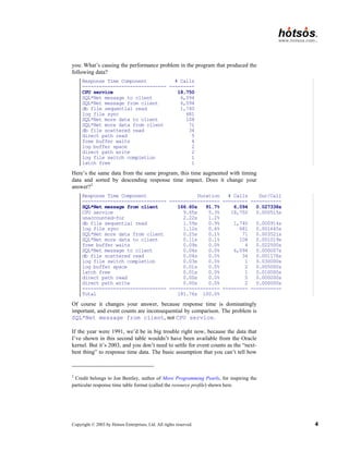
Copyright © 2003
by Hotsos Enterprises, Ltd. All rights reserved. 4 you: What’s causing the performance problem in the program that produced the following data? Response Time Component # Calls ------------------------------ --------- CPU service 18,750 SQL*Net message to client 6,094 SQL*Net message from client 6,094 db file sequential read 1,740 log file sync 681 SQL*Net more data to client 108 SQL*Net more data from client 71 db file scattered read 34 direct path read 5 free buffer waits 4 log buffer space 2 direct path write 2 log file switch completion 1 latch free 1 Here’s the same data from the same program, this time augmented with timing data and sorted by descending response time impact. Does it change your answer?2 Response Time Component Duration # Calls Dur/Call ------------------------------ ------------------ --------- ----------- SQL*Net message from client 166.60s 91.7% 6,094 0.027338s CPU service 9.65s 5.3% 18,750 0.000515s unaccounted-for 2.22s 1.2% db file sequential read 1.59s 0.9% 1,740 0.000914s log file sync 1.12s 0.6% 681 0.001645s SQL*Net more data from client 0.25s 0.1% 71 0.003521s SQL*Net more data to client 0.11s 0.1% 108 0.001019s free buffer waits 0.09s 0.0% 4 0.022500s SQL*Net message to client 0.04s 0.0% 6,094 0.000007s db file scattered read 0.04s 0.0% 34 0.001176s log file switch completion 0.03s 0.0% 1 0.030000s log buffer space 0.01s 0.0% 2 0.005000s latch free 0.01s 0.0% 1 0.010000s direct path read 0.00s 0.0% 5 0.000000s direct path write 0.00s 0.0% 2 0.000000s ------------------------------ ------------------ --------- ----------- Total 181.76s 100.0% Of course it changes your answer, because response time is dominatingly important, and event counts are inconsequential by comparison. The problem is SQL*Net message from client, not CPU service. If the year were 1991, we’d be in big trouble right now, because the data that I’ve shown in this second table wouldn’t have been available from the Oracle kernel. But it’s 2003, and you don’t need to settle for event counts as the “next- best thing” to response time data. The basic assumption that you can’t tell how 2 Credit belongs to Jon Bentley, author of More Programming Pearls, for inspiring the particular response time table format (called the resource profile) shown here.
5.
Copyright © 2003
by Hotsos Enterprises, Ltd. All rights reserved. 5 long the Oracle kernel takes to do things is simply incorrect, and it has been since 1992—since Oracle Release 7.0.12. Amdahl’s Law The final “great advance” in Oracle performance optimization that I’ll mention is an observation made thirty-six years ago by Gene Amdahl, in 1967. To paraphrase the statement that became known as Amdahl’s Law: Performance improvement is proportional to how much a program uses the thing you improved. Amdahl’s Law is why you should view response time components in descending response time order. In the example from the previous section, it’s why you don’t work on the CPU service “problem” before figuring out the SQL*Net message from client problem. If you were to reduce CPU consumption by 50%, you’d improve response time by only about 2%. But if you could reduce the response time attributable to SQL*Net message from client by the same 50%, you’ll reduce total response time by 46%. In this example, each percentage point of reduction in SQL*Net message from client duration produces nearly twenty times the impact of a percentage point of CPU service reduction. Amdahl’s Law is a formalization of optimization common sense. It tells you how to get the biggest bang for the buck for your performance improvement efforts. All Together Now Combining the three advances in Oracle optimization technology into one statement results in the following simple performance method: Work first to reduce the biggest response time component of a business’ most important user action. It sounds easy, right? Yet I can be almost certain that this is not how you optimize your Oracle system back home. It’s not what your consultants do or what your tools do, and this way of “tuning” is nothing like how your books or virtually any of the other papers presented at Oracle seminars and conferences since 1980 tell you to do. So what is the missing link? The missing link is that unless you know how to extract and interpret response time measurements from your Oracle system, you can’t implement this simple optimization method. Explaining how to extract and interpret response time measurements from your Oracle system is the point of this paper.
6.
Copyright © 2003
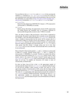
by Hotsos Enterprises, Ltd. All rights reserved. 6 Quick Tour of Extended SQL Trace Data When you hear about the “important feature first published in Oracle 7.0.12,” you probably think of the so-called wait interface. And when you hear the term wait interface, you’re probably conditioned to think of V$SESSION_WAIT, V$SESSION_EVENT, and V$SYSTEM_EVENT. However, I’m not going to go there in this paper. Instead, I’ll begin my discussion of Oracle operational timing data by offering a brief introduction to Oracle’s extended SQL trace facility. Oracle’s extended SQL trace facility is a much easier educational vehicle for describing the kernel’s operational timing data. And, for reasons I’ll describe later, the extended SQL trace facility is in many ways a more practical tool than the V$ fixed views anyway. Activating Extended SQL Trace There are many ways to activate extended SQL trace. The easiest and most reliable is to insert a few lines of SQL into your source code, as follows: alter session set timed_statistics=true alter session set max_dump_file_size=unlimited alter session set tracefile_identifier='POX20031031a' alter session set events '10046 trace name context forever, level 8' /* code to be traced goes here */ alter session set events '10046 trace name context off' In this example, I’ve activated Oracle’s extended SQL trace facility at level 8, which will cause the Oracle kernel to emit detailed timing data for both database calls and the so-called wait events motivated by those database calls. It is also possible to activate extended SQL tracing for programs to which you do not have the ability to insert SQL commands into the program source code. For example, Oracle’s SYS.DBMS_SUPPORT.START_TRACE_IN_SES- SION procedure gives you this capability. Activating extended SQL trace from a session other than the one being traced introduces complications into the data collection process, but these complications can be detected and corrected [Millsap (2003)]. Finding the Trace File Finding your trace file is trivial if you were able to insert the ALTER SESSION SET TRACEFILE_IDENTIFIER directive into your source code. In the example shown here, I’ve used the string POX20031031a as an identifier to help identify my trace file. The code I’ve conjured up refers perhaps to the first “POX” report traced on 31 October 2003. On my OFA-compliant Linux system,
7.
Copyright © 2003
by Hotsos Enterprises, Ltd. All rights reserved. 7 this directive would result in a trace file named something like $ORACLE_BASE/admin/test9/udump/ora_2136_POX20031031a.trc.3 If you’re unable to use the TRACEFILE_IDENTIFIER trick (for example, because you’re using a release of Oracle prior to 8.1.7, or because you’re activating trace from a third-party session), then you can generally identify your trace file by searching the appropriate trace file directory (the value of USER_DUMP_DEST for most trace files) for files with appropriate mtime values. You can identify the right trace file with certainty by confirming that the pid value recorded inside your trace file matches the value of V$PROCESS.SPID for the session you were tracing (instead of a pid value, you’ll find a thread_id value on Oracle for Microsoft Windows ports). Trace File Walk-Through The attribute that makes extended SQL trace data so educationally significant is that a trace file contains a complete chronological history of how a database session spent its time. It is extremely difficult to do this with V$ data, but completely natural with trace data. Extended SQL trace data contain many interesting elements, but the ones of most interest for the purpose of this paper are lines of the forms: PARSE #54:c=20000,e=11526,p=0,cr=2,cu=0,mis=1,r=0,dep=1,og=0,tim=1017039304725071 EXEC #1:c=10000,e=12137,p=0,cr=22,cu=0,mis=0,r=1,dep=0,og=4,tim=1017039275981174 FETCH #3:c=10000,e=306,p=0,cr=3,cu=0,mis=0,r=1,dep=2,og=4,tim=1017039275973158 WAIT #1: nam='SQL*Net message to client' ela= 40 p1=1650815232 p2=1 p3=0 WAIT #1: nam='SQL*Net message from client' ela= 1709 p1=1650815232 p2=1 p3=0 WAIT #34: nam='db file sequential read' ela= 14118 p1=52 p2=2755 p3=1 WAIT #44: nam='latch free' ela= 1327989 p1=-1721538020 p2=87 p3=13 Although I’ve shown several examples, the lines shown here actually take on two forms: database calls, which begin with tokens like PARSE, EXEC, and FETCH; and so-called wait events, which begin with the token WAIT. Note that all database call lines take on the same format, just with different numbers plugged into the fields; and that all wait event lines take on another consistent format, just with different values for each line’s string and numeric fields. I won’t distract you with definitions for all the fields here. The most important ones for you to understand for the purposes of this paper are: #n n is the id of the cursor upon which the database call or wait event is acting. c The approximate total CPU capacity (user-mode plus kernel-mode) consumed by the database call. 3 Thanks to Julian Dyke for bringing the new (8.1.7) TRACEFILE_IDENTIFIER parameter to my attention.
8.
Copyright © 2003
by Hotsos Enterprises, Ltd. All rights reserved. 8 e The approximate wall clock time that elapsed during the database call. nam The name assigned by an Oracle kernel developer to a sequence of instructions (often including a system call) in the Oracle kernel. ela The approximate wall clock time that elapsed during the wait event. You can read about all the other fields by downloading Oracle MetaLink note 39817.1. Wait events represented in an Oracle trace file fall into two categories: • Wait events that were executed within database calls, and • Wait events that were executed between database calls. You can distinguish between the two types by the value of the nam field. Commonly occurring wait events that occur between database calls include the following: SQL*Net message from client SQL*Net message to client single-task message pipe get rdbms ipc message pmon timer smon timer Most other wait events are executed within database calls. It is important to distinguish properly between the two types of wait events because failing to do so leads to incorrect time accounting. For a single database call, the call’s total wall time (e value) approximately equals the sum of the call’s CPU service time (c value) plus the sum of all the wall time attributable to wait events executed by that database call (the sum of the relevant ela values). Or, formally, you can write: db call e c ela ≈ + ∑ . The Oracle kernel emits information for an action when the action completes. Therefore, the wait events for a given cursor action appear in the trace data stream in advance of the database call that executed the wait events. For example, if a fetch call were to issue two OS read calls, you would see something like the following in the trace file: WAIT #4: nam='db file sequential read' ela= 13060 p1=1 p2=53903 p3=1 WAIT #4: nam='db file sequential read' ela= 6978 p1=1 p2=4726 p3=1
9.
Copyright © 2003
by Hotsos Enterprises, Ltd. All rights reserved. 9 FETCH #4:c=0,e=21340,p=2,cr=3,cu=0,mis=0,r=0,dep=1,og=4,tim=1033064137953092 These two wait events were executed within the fetch shown on the third line. Notice the presence here of the relationship that I mentioned a moment ago: { } db call 21340 0 13060, 6978 20038. e c ela ≈ + ≈ + = ∑ ∑ . However, for wait events executed between db calls, the wait event duration does not roll up into an elapsed duration for any database call. For example: PARSE #9:c=0,e=0,p=0,cr=0,cu=0,mis=1,r=0,dep=0,og=4,tim=1716466757 WAIT #9: nam='SQL*Net message to client' ela= 0 p1=1413697536 p2=1 p3=0 WAIT #9: nam='SQL*Net message from client' ela= 3 p1=1413697536 p2=1 p3=0 ... PARSE #9:c=0,e=0,p=0,cr=0,cu=0,mis=0,r=0,dep=0,og=4,tim=1716466760 As you can see, the e=0 value for the second parse call does not contain the ela=0 and ela=3 values for the two wait events that precede it. I’ve described the relationship among the c, e, and ela statistics related to a single database call. It’s a slightly more complicated matter to derive the relationship among c, e, and ela for an entire trace file, but the result becomes intuitive after examining a few trace files. The following relationship relates the total response time (called R in the following relation) represented by a trace file to the c, e, and ela statistics within a trace file: 0 between calls 0 within between calls calls 0 . dep dep dep R e ela c ela ela c ela = = = = + ≈ + + = + ∑ ∑ ∑ ∑ ∑ ∑ ∑ One complication that I will not detail here is the importance of the dep=0 constraint on the sum of the c statistic values. Suffice it to say that this prevents double-counting, because c values at non-zero recursive depths are rolled up into the statistics for their recursive parents. The value in understanding the two mathematical relationships that I’ve shown here is that, with them, you can construct a perfect resource profile—a table listing response time components in descending order of importance like the one shown above in “Response Time Focus”—from an extended SQL trace file.
10.
Copyright © 2003
by Hotsos Enterprises, Ltd. All rights reserved. 10 Such a capability, of course, enables you to use the suspiciously simple yet completely reliable performance optimization method that I described earlier: Work first to reduce the biggest response time component of a business’ most important user action. With c, e, and ela, you can do it. Oracle Timing Instrumentation Oracle performance analysts often underutilize extended SQL trace data or even discard useful data entirely, because they don’t trust it. The aim of this section is to explain a couple of research results that my staff and I have derived since the year 2000, which greatly improve the practical usefulness of Oracle’s extended SQL trace data. What the Oracle Kernel Actually Measures Before you can understand what the c, e, and ela statistics really mean, it is helpful to understand where they come from. The Oracle kernel computes these statistics based on the results of system calls that, on Linux, look like this: procedure dbcall { e0 = gettimeofday; # mark the wall time c0 = getrusage; # obtain resource usage statistics ... # execute the db call (may call wevent) c1 = getrusage; # obtain resource usage statistics e1 = gettimeofday; # mark the wall time e = e1 – e0; # elapsed duration of dbcall c = (c1.utime + c1.stime) – (c0.utime + c0.stime); # total CPU time consumed by dbcall print(TRC, ...); # emit PARSE, EXEC, FETCH, etc. line } procedure wevent { ela0 = gettimeofday; # mark the wall time ... # execute the wait event here ela1 = gettimeofday; # mark the wall time ela = ela1 – ela0; # ela is the duration of the wait event print(TRC, "WAIT..."); # emit WAIT line } Oracle for Linux uses calls to the POSIX-compliant system calls named gettimeofday and getrusage for its timing information. You can figure out which system calls your Oracle kernel uses by executing a system call tracing tool like Linux’s strace tool. You can find such a tool for your system by visiting http://www.pugcentral.org/howto/truss.htm.
11.
Copyright © 2003
by Hotsos Enterprises, Ltd. All rights reserved. 11 You can find out what gettimeofday and getrusage do by executing the standard man command (e.g., man gettimeofday) on any Unix system. If your operating system lacks good system call documentation, then you can find the information you need online at http://www.unix-systems.org/single_unix_- specification. Conceptually, gettimeofday and getrusage are simple: gettimeofday Return the time elapsed since 00:00:00 UTC, January 1, 1970, expressed in microseconds (1/1,000,000th of a second). getrusage Return, among other things, the approximate amount of CPU capacity that the calling process has consumed since its invocation, expressed in microseconds (but generally accurate to only 1/100th of a second). Now, one thing to realize is that just because a unit of time is expressed in microseconds, this doesn’t mean that the time is accurate to one microsecond. For example, a call to the Microsoft Windows gettimeofday function will return a number of microseconds, but the answer will be accurate only to a centisecond (1/100th of a second). On the same hardware, a call to the Linux gettimeofday function will return an answer accurate to a microsecond. However, unless you recompile your Linux kernel with _SC_CLK_TCK set to a value greater than 100, (which I strongly advise you not to do), then getrusage even on Linux will return microsecond data that is accurate only to one centisecond. Prior to Oracle9i, Oracle kernels printed c, e, and ela statistics in centiseconds (1/100th of a second). Oracle9i kernels print c, e, and ela statistics in microseconds (1/1,000,000th of a second). Therefore on systems that deliver better-than-centisecond resolution for gettimeofday, Oracle version 7 and 8 kernels round to the nearest 0.01 second. Version 9 kernels print the full gettimeofday and getrusage result in microseconds, even if the last four digits are all zero. To simplify our discussion, let’s speak in terms of microseconds, as Oracle9i does. So what we know from all this is that e is the approximate number of microseconds that elapses between gettimeofday calls that bracket the guts of a db call (for example, a parse, execute, or fetch). The value of c is the approximate number of microseconds of CPU service that the Oracle kernel consumed between the getrusage calls that bracket the guts of the db call. The value of c is a particularly weak approximation, because the resolution of getrusage is limited to 10,000 microseconds. And finally the value of ela is the approximate number of microseconds that elapses between the gettimeofday calls that bracket the guts of an instrumented OS call made by the Oracle kernel.
12.
Copyright © 2003
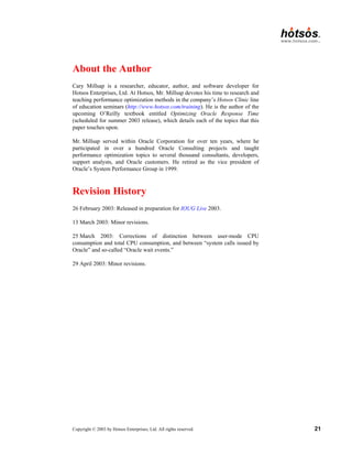
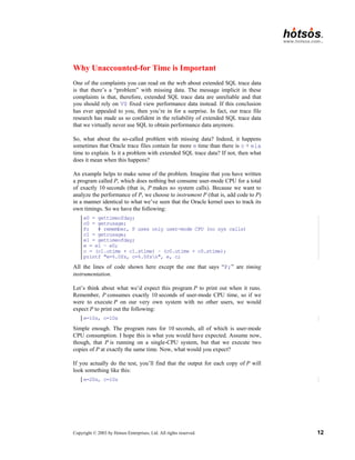
by Hotsos Enterprises, Ltd. All rights reserved. 12 Why Unaccounted-for Time is Important One of the complaints you can read on the web about extended SQL trace data is that there’s a “problem” with missing data. The message implicit in these complaints is that, therefore, extended SQL trace data are unreliable and that you should rely on V$ fixed view performance data instead. If this conclusion has ever appealed to you, then you’re in for a surprise. In fact, our trace file research has made us so confident in the reliability of extended SQL trace data that we virtually never use SQL to obtain performance data anymore. So, what about the so-called problem with missing data? Indeed, it happens sometimes that Oracle trace files contain far more e time than there is c + ela time to explain. Is it a problem with extended SQL trace data? If not, then what does it mean when this happens? An example helps to make sense of the problem. Imagine that you have written a program called P, which does nothing but consume user-mode CPU for a total of exactly 10 seconds (that is, P makes no system calls). Because we want to analyze the performance of P, we choose to instrument P (that is, add code to P) in a manner identical to what we’ve seen that the Oracle kernel uses to track its own timings. So we have the following: e0 = gettimeofday; c0 = getrusage; P; # remember, P uses only user-mode CPU (no sys calls) c1 = getrusage; e1 = gettimeofday; e = e1 – e0; c = (c1.utime + c1.stime) – (c0.utime + c0.stime); printf "e=%.0fs, c=%.0fsn", e, c; All the lines of code shown here except the one that says “P;” are timing instrumentation. Let’s think about what we’d expect this program P to print out when it runs. Remember, P consumes exactly 10 seconds of user-mode CPU time, so if we were to execute P on our very own system with no other users, we would expect P to print out the following: e=10s, c=10s Simple enough. The program runs for 10 seconds, all of which is user-mode CPU consumption. I hope this is what you would have expected. Assume now, though, that P is running on a single-CPU system, but that we execute two copies of P at exactly the same time. Now, what would you expect? If you actually do the test, you’ll find that the output for each copy of P will look something like this: e=20s, c=10s
13.
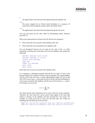
Copyright © 2003
by Hotsos Enterprises, Ltd. All rights reserved. 13 We now have a “problem with missing time.” Where did the other 10 seconds go? If we weren’t intimately familiar with P, then we would probably guess that the 10 seconds of time that was not user-mode CPU consumption was probably consumed by system calls. But we wrote P ourselves, and we know that P makes no system calls whatsoever. So what is wrong with our instrumentation? How could we have improved our instrumentation so that we wouldn’t have a missing time problem? The answer is that we’ve really done nothing wrong. Here’s what happened. Two copies of P running concurrently each requested 10 seconds’ worth of user-mode CPU. The operating system on our computer tried to oblige both requests, but there’s only a limited amount of CPU capacity to go around (one CPU’s worth, to be exact). The operating system dutifully time-sliced CPU requests in 0.01-second increments (if _SC_CLK_TCK=100), and it simply took 20 seconds of elapsed time for the CPU to supply 10 seconds’ worth of capacity to each of the two copies of P (plus perhaps an additional few microseconds for the operating system to do its scheduling work, plus the time consumed by gettimeofday and getrusage calls). The missing time that each copy of P couldn’t account for is simply time that the program spent not executing. Literally, it was time spent outside of the user running and kernel running states in the process state transition diagram shown in Figure 1. 1 user running 3 ready to run 4 asleep sys call, interrupt schedule process wakeup context switch permissible sleep interrupt return return interrupt 2 kernel running preempt Figure 1. An operating system process state diagram [Bach (1986) 31].
14.
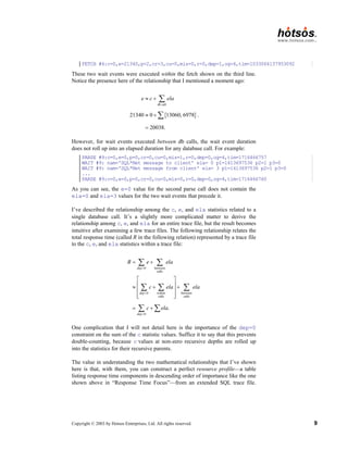
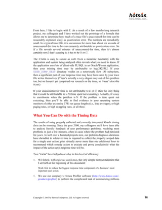
Copyright © 2003
by Hotsos Enterprises, Ltd. All rights reserved. 14 This is one possible source of missing Oracle time data. But there are others as well. For example, every timing measurement obtained from a digital clock can contain up to one clock resolution unit’s worth of error, called quantization error. You might have seen such small discrepancies in trace data timings before and thought of them as “rounding error.” Figure 2 shows two examples of quantization error: time em = 1 1512 1513 1514 1515 1516 1517 1518 1519 ea = 0.25 e'a = 0.9375 e'm = 0 Figure 2. Quantization error [Millsap (2003)]. In the top case, the actual duration of some software event was ea = 0.25, one quarter of a clock tick. However, the event happened to cross a clock tick, so the beginning and ending gettimeofday values differed by one. The result: the measured duration of the event was em = 1 clock tick. Total quantization error in this case is E = em – ea = 1 – 0.25 = 0.75 clock ticks, which is a whopping 300% of the actual event duration. In the bottom case, the actual event duration was e′a = 0.9375, but we can’t know this by measuring with the digital clock shown here. We can only know that the gettimeofday values obtained immediately before and immediately after the event were the same, so the measured duration was e′m = 0 clock ticks. Total quantization error in this case is E′ = e′m – e′a = 0 – 0.9375 = −0.9375 clock ticks. Again, as a percentage of the actual event duration, this error is enormous: it’s −100% of e′a. However, when summing over large numbers of measurements, total quantization error tends to sum to zero. It is of course possible that the stars could line up in an unlucky way, and that a thousand straight quantization errors could all aggregate in one direction or another, but the chances are remote, and the exact probability of such events is in fact easy to compute.
15.
Copyright © 2003
by Hotsos Enterprises, Ltd. All rights reserved. 15 So now I have described two sources of “missing” or “unaccounted-for” trace file time. A third source is un-instrumented segments of Oracle kernel code. There are certain operations within the Oracle kernel that Oracle kernel developers simply don’t instrument in the way shown in the procedure wevent pseudocode shown above. One example is the write system call that the Oracle kernel uses to write trace data to the trace file. Another example is that Oracle doesn’t instrument the kernel’s system timer calls either (it would be silly to put gettimeofday calls around every gettimeofday call!). This special case of systematic instrumentation error is called measurement intrusion error. The error introduced by factors like these is usually small. There are other cases, such as the one described in bug number 2425312 at Oracle MetaLink, that can rack up hours’ worth of unaccounted-for time. The solution to this one is an Oracle kernel patch. Isn’t it catastrophic news for the trace file enthusiast that there are several categories of error in the response time equation for a trace file? Essentially, this means that for a whole trace file’s response time, we have the following single equation in several unknowns: 0 dep R c ela M E N U S = = + + + + + + ∑ ∑ . In this equation, M denotes the measurement intrusion error, E is total quantization error, N denotes the time spent not executing, U is the time consumed by un-instrumented system calls, and S is a category I haven’t discussed in this document: the effect of double-counted CPU time [Millsap (2003)]. How can we possibly isolate the values of M, E, N, U, and S when we have only one equation defining their relationship? Mathematically it sounds bad, but it really isn’t. First, the practical need to isolate M, E, N, U, and S is actually rare. You won’t even want to solve the puzzle unless “unaccounted-for” is one of the top (50% or more) consumers of your user action’s total response time, and this probably won’t happen to you very often. However, without being able to isolate M, E, N, U, and S in this case, the simple method I described in the first section of this paper would be unreliable for certain performance problem types. The good news is that there is a repeatable method you can use to isolate M, E, N, U, and S. First, it is generally safe to ignore the effects of M and S. The total effects of measurement intrusion error account for only a few microseconds of time consumption per timed event (whether database call or wait event). Consequently, its effect is nearly always negligible. Experience at hotsos.com with several hundreds of trace files indicates that the verdict on S (CPU double- counting, explained in [Millsap (2003)] is identical: nearly always negligible. This reduces our five-variable equation to an equation in three variables.
16.
Copyright © 2003
by Hotsos Enterprises, Ltd. All rights reserved. 16 From here, I like to begin with E. As a result of a few months-long research project, my colleagues and I have worked out the prototype of a formula that allows me to determine how much of a trace file’s unaccounted-for time can be reasonably explained away as quantization error. The numbers are remarkably small. In a typical trace file, it is uncommon for more than about ten seconds of unaccounted-for time to be even remotely attributable to quantization error. So if a file reveals several minutes of unaccounted-for time, then it’s almost certainly not E that’s causing it; it has to be N or U. The U term is easy to isolate as well. Even a moderate familiarity with the application and system being analyzed often reveals what you need to know. If the application uses lots of client-side PL/SQL in an Oracle*Forms application, then your missing time may be attributable to bug 2425312. If your USER_DUMP_DEST directory resides on a notoriously slow I/O subsystem, then a significant part of your response time may have been eaten by your trace file writes themselves. (There’s actually a very elegant way out of this problem too, but we haven’t yet completed our research on the issue, so I won’t describe it yet.) If your unaccounted-for time is not attributable to E or U, then the only thing that it could be attributable to is N (time spent not executing). Actually, it’s easy to corroborate when the problem is N. If the problem is time spent not executing, then you’ll be able to find evidence in your operating system monitors of either excessive CPU run queue lengths (i.e., load averages), or high paging rates, or high swapping rates, or all three. What You Can Do with the Timing Data The results of using properly collected and correctly interpreted Oracle timing data can be stunning. Since the year 2000, my colleagues and I have been able to analyze literally hundreds of user performance problems, resolving most problems in just a few minutes, often in cases where the problem had persisted for years. In well over a hundred projects now, our problem diagnosis durations have dwindled to whatever time is required to collect the properly scoped data for a single user action, plus virtually never more than one additional hour to recommend which remedy action to execute and prove conclusively what the impact of the action upon response time will be. Two “tricks” have helped us evolve to this level of efficiency: 1. We follow, with rigorous conviction, the very simple method statement that I set forth at the beginning of this document: Work first to reduce the biggest response time component of a business’ most important user action. 1. We use our company’s Hotsos Profiler software (http://www.hotsos.com/- products/profiler) to perform the complicated task of summarizing millions
17.
Copyright © 2003
by Hotsos Enterprises, Ltd. All rights reserved. 17 of lines of trace data. In some cases, Oracle’s tkprof and trace file analyzer tools will work just fine. In many cases we’ve experienced, the Hotsos Profiler has saved several hours of tedious manual labor per project. In our field work, this method has proven extraordinarily efficient and reliable enough to warrant the claim that performance problems simply cannot hide from this method. In hundreds of problems solved since 2000, our successes have included efficient resolution in dozens of different problem types, including: • Slow user actions whose problem root causes were system-wide inefficiencies, and slow user actions whose performance problem root causes could never have been determined from system-wide data analysis (like the Oracle Payroll problem described in the text). • All sorts of query inefficiencies including SQL statements that accidentally prevented the use of good access paths, missing or redundant indexes, and data density issues. • Application design or implementation mistakes such as client code that issues more parse calls than necessary, fails to share SQL through bind variable use, or that fails to use efficient array processing features. • Serialization issues such as contention for locks, latches, or memory buffers, whose root causes range typically from poor transaction design to inefficient SQL or application code design. • Network configuration mistakes such as inefficient SQL*Net protocol selection, faulty network segments, and inefficient topology design. • CPU and memory capacity shortages resulting in swapping, paging, or just excessive context switching. • Disk I/O issues such as poorly sized cache allocations, I/O subsystem design inefficiencies, and imbalanced I/O loads Tracing versus Polling I mentioned earlier that I like trace data because it presents a simple interface to the complete history of where a user action’s response time has gone. To acquire the same historical record from Oracle’s V$ fixed views would require polling. The extended SQL trace mechanism is an event-based tracing tool which emits data only when an interesting system state change occurs. With fixed view data, there’s no event-based means of accessing the data; you simply have to poll for it. There’s a big problem with polling; well, actually, there are two big problems.
18.
Copyright © 2003
by Hotsos Enterprises, Ltd. All rights reserved. 18 1. First, if you poll too infrequently, you miss important state changes. For example, if you poll every second for event completions in V$SESSION_EVENT, you’ll never even notice at least 99% of events that consume 0.01 seconds or less. How would you like a data collection mechanism that guaranteed that you miss detecting 99% or more of the disk I/O events your user action motivates? 2. Second, if you poll too frequently, you waste the same system resources that you need more of to make your application run faster. For example, if you poll 100 times per second for event completions in V$SESSION_EVENT, you’ll burn so much CPU that your application monitoring tool will become the most expensive application on the system. As much as you’d like to sample your V$ data 100 times or more per second, you simply can’t—at least not with SQL. Try it. See how many times you can select data from V$SESSION_EVENT in a tight loop within one second. You’ll be lucky if you can grab the data more than 50 times a second for any system with at least a few dozen Oracle sessions connected. If you’re going to poll with sufficient frequency, you simply have to go with code that attaches itself directly to the Oracle system global area (SGA). It’s of course possible to do this: Precise, Quest, and even Oracle all do it. It’s of course more difficult than accessing the data through SQL. Because we’ve had such spectacular success with extended SQL trace data, my company has not yet found the motivation to make the investment into polling directly from the Oracle SGA. Why I Use Extended SQL Trace Data Instead of Oracle’s V$ Fixed Views One thing that the V$ fixed views are extraordinarily good at is providing snapshots of either system-wide or session-wide activity. You should regard any system-wide data as highly suspect, for reasons illustrated in the earlier section describing the importance of user action focus. However, analyzing the difference between successive snapshots of the appropriate union of V$SESSTAT and V$SESSION_EVENT can give useful results for many situations [Millsap (2003)]. Tom Kyte, Jonathan Lewis, and Steve Adams all use similar techniques to determine “what happened” between snapshots. However, it is difficult to create a very sharp-edged software tool using snapshots of V$ data. I invested nearly half of the year 2000 into reproducing the results we can acquire from extended SQL trace data, using only Oracle V$ data. The problems are complicated to explain (the current draft of some of the explanations already consumes several pages in my book project manuscript), but here is a taste:
19.
Copyright © 2003
by Hotsos Enterprises, Ltd. All rights reserved. 19 • The worst problem is that there are just too many data sources. It’s not just V$SESSTAT and V$SESSION_EVENT. What if you find out from those sources that your performance problem is latch contention? Oops, you wish you had polled and stored data from V$LATCH as well. What if you find a buffer busy waits problem? Oops, you wish you had polled and stored data from V$WAITSTAT. The final list contains dozens of data sources, which creates a virtually impossible problem if you’re trying to collect all the performance data you needed without asking a user to run a painful user action a second time—while you “collect more data.” With trace data you simply don’t have to worry about the problem, because all the relevant details about what the user action waited on are right there in the trace file. • There’s no notion of e (db call elapsed time) in the Oracle fixed views. Consequently, you can’t tell whether there’s unaccounted-for time or not. Remember the argument that trace data is inferior to V$ data because of the “missing time problem?” Well, the V$ data suffers from the same missing time problem, only it’s worse: you can’t even tell that there is missing time, which precludes any possibility of using the useful N, E, U analysis technique that I described previously. • Data obtained from Oracle shared memory is not read consistent, even if you use SQL upon the V$ views. This causes problems that are fare more interesting and exciting than a guy my age should have to cope with. • The value of the statistic called CPU time used by this session is unreliable. This makes it more difficult to figure out the value of c (user- mode CPU consumption) for a session. • The information in V$SESSION_WAIT.SECONDS_IN_WAIT is not granular enough to be useful. Because the Oracle kernel updates this column only roughly every three seconds, it is virtually impossible to determine when an in-process event began (unless you poll with sufficient frequency, directly from the SGA). • Oracle event counts and timers are susceptible to overflow. It takes smart, port-aware code to figure out what to do when a newly obtained event count is a smaller value than an earlier one. • There is no way to determine the recursive relationships among cursor actions by looking at V$ data. This makes it intensely difficult to attribute response time consumption to the appropriate places in your application source code that demand attention. Imagine that you have found that the source of your performance problem is the SQL statement “BEGIN f(6); END;”… I have spent hours trudging through DBA_SOURCE and other dictionary tables trying to track down all the relationships among SQL statements in an application. It’s possible to automate the process by correctly parsing an Oracle trace file (this is one of the best time-saving features of the Hotsos Profiler).
20.
Copyright © 2003
by Hotsos Enterprises, Ltd. All rights reserved. 20 • The transient nature of Oracle sessions increases the difficulty too. If your session ends before the second snapshot can be obtained, then the only way you can collect the data you need is to begin the problem user action again. Why don’t I use V$ data anymore? Because it’s a mess. It’s far less efficient than the alternative. If I can get my hands on the right extended SQL trace data, I can solve a performance problem so much more quickly than if I have to fight through all the doubt introduced by V$ complexities like the ones I’ve described here. And I almost always can get my hands on the right extended SQL trace data, because on projects we work on, we require it with rigorous conviction. The method enabled by collecting properly scoped extended SQL trace data really is that good. References Bach, M. 1986. The Design of the Unix Operating System. Prentice-Hall. Bentley, J. 1988. More Programming Pearls: Confessions of a Coder. Addison- Wesley. Kolk, A.; Yamaguchi, S.; Viscusi, J. 1999. Yet Another Performance Profiling Method (or YAPP Method). Oracle Corp. Millsap, C. 2003. Optimizing Oracle Response Time. O’Reilly. Estimated publication date July 2003. Acknowledgments I’d like to thank all the standard folks for their contribution to the body of work I’m adding to: Anjo Kolk for introducing me to so many of the concepts contained in this paper and for being there any time I’ve needed; Mogens Nørgaard and Virag Saksena for forcing me to see the value of response time optimization; Juan Loaiza for instrumenting the Oracle kernel with timing data in the first place; Gaja Krishna Vaidyanatha and Kirti Deshpande for breaking into the book market with the news; Jeff Holt for creating the Hotsos Profiler and teaching me virtually everything I know in this my incarnation as a scientist; Gary Goodman and the Hotsos customers he has found, for helping me feed my family while I have the time of my life teaching and doing research; and my beautiful wife and children—Mindy, Alex, and Nik—for their patience, devotion, and sense of what’s really important.
21.
Copyright © 2003
by Hotsos Enterprises, Ltd. All rights reserved. 21 About the Author Cary Millsap is a researcher, educator, author, and software developer for Hotsos Enterprises, Ltd. At Hotsos, Mr. Millsap devotes his time to research and teaching performance optimization methods in the company’s Hotsos Clinic line of education seminars (http://www.hotsos.com/training). He is the author of the upcoming O’Reilly textbook entitled Optimizing Oracle Response Time (scheduled for summer 2003 release), which details each of the topics that this paper touches upon. Mr. Millsap served within Oracle Corporation for over ten years, where he participated in over a hundred Oracle Consulting projects and taught performance optimization topics to several thousand consultants, developers, support analysts, and Oracle customers. He retired as the vice president of Oracle’s System Performance Group in 1999. Revision History 26 February 2003: Released in preparation for IOUG Live 2003. 13 March 2003: Minor revisions. 25 March 2003: Corrections of distinction between user-mode CPU consumption and total CPU consumption, and between “system calls issued by Oracle” and so-called “Oracle wait events.” 29 April 2003: Minor revisions.
Download

![Copyright © 2003 by Hotsos Enterprises, Ltd. All rights reserved. 3
program’s total 1,985.40-second execution time, only 23.69 seconds were
consumed waiting on latches. The ironic thing is that even if the company had
completely eradicated waits for latch free from the face of their system,
they would have made only a 1.2% performance improvement in the response
time of their payroll program.
How could this happen? The non-payroll workload had serious enough latch
free problems that it influenced the system-wide average. But it was a grave
error to assume that the payroll program’s problem was the same as the system-
wide average problem. The error cost the company three months of wasted time
and frustration and who knows how much labor and equipment upgrade cost.
By contrast, diagnosing the real payroll performance problem consumed only
about ten minutes of diagnosis time once the company saw the correct data.
My colleagues and I encounter this type of problem repeatedly. The solution is
for you (the performance analyst) to focus entirely upon the user actions that
need optimizing. The business can tell you what the most important user actions
are. The system cannot. Once you have identified the user actions that require
optimization, then your first job is to collect operational data exactly for that
user action: no more, and no less.
Response Time Focus
For a couple of decades now, Oracle performance analysts have labored under
the assumption that there’s really no objective way to measure Oracle response
times. In the perceived absence of objective response time measurements,
analysts have settled for the next-best thing: event counts. And of course from
event counts come ratios. And from ratios come all sorts of arguments about
what “tuning” actions are important, and what ones are not.
However, users don’t care about event counts and ratios and arguments; they
care about response time.1
No matter how much complexity you build atop any
timing-free event-count data, you are fundamentally doomed by the following
inescapable truth. My second important advance is the following observation:
You can’t tell how long something took by counting how
many times it happened.
Users care only about response times. If you’re measuring only event counts,
then you’re not measuring anything the users care about. Here’s another quiz for
1
Thanks to Anjo Kolk for giving us the now-famous YAPP Method [Kolk et al. (1999)],
which served many in our industry as the first hope that measuring Oracle response times
objectively was even possible.](https://image.slidesharecdn.com/oracleoperationaltimingdata-251115015111-4f357c79/85/Oracle-Operational-Timing-Data-for-performance-tuning-3-320.jpg)
![Copyright © 2003 by Hotsos Enterprises, Ltd. All rights reserved. 6
Quick Tour of Extended SQL Trace Data
When you hear about the “important feature first published in Oracle 7.0.12,”
you probably think of the so-called wait interface. And when you hear the term
wait interface, you’re probably conditioned to think of V$SESSION_WAIT,
V$SESSION_EVENT, and V$SYSTEM_EVENT. However, I’m not going to go
there in this paper. Instead, I’ll begin my discussion of Oracle operational
timing data by offering a brief introduction to Oracle’s extended SQL trace
facility. Oracle’s extended SQL trace facility is a much easier educational
vehicle for describing the kernel’s operational timing data. And, for reasons I’ll
describe later, the extended SQL trace facility is in many ways a more practical
tool than the V$ fixed views anyway.
Activating Extended SQL Trace
There are many ways to activate extended SQL trace. The easiest and most
reliable is to insert a few lines of SQL into your source code, as follows:
alter session set timed_statistics=true
alter session set max_dump_file_size=unlimited
alter session set tracefile_identifier='POX20031031a'
alter session set events '10046 trace name context forever, level 8'
/* code to be traced goes here */
alter session set events '10046 trace name context off'
In this example, I’ve activated Oracle’s extended SQL trace facility at level 8,
which will cause the Oracle kernel to emit detailed timing data for both database
calls and the so-called wait events motivated by those database calls.
It is also possible to activate extended SQL tracing for programs to which you
do not have the ability to insert SQL commands into the program source code.
For example, Oracle’s SYS.DBMS_SUPPORT.START_TRACE_IN_SES-
SION procedure gives you this capability. Activating extended SQL trace from
a session other than the one being traced introduces complications into the data
collection process, but these complications can be detected and corrected
[Millsap (2003)].
Finding the Trace File
Finding your trace file is trivial if you were able to insert the ALTER SESSION
SET TRACEFILE_IDENTIFIER directive into your source code. In the
example shown here, I’ve used the string POX20031031a as an identifier to
help identify my trace file. The code I’ve conjured up refers perhaps to the first
“POX” report traced on 31 October 2003. On my OFA-compliant Linux system,](https://image.slidesharecdn.com/oracleoperationaltimingdata-251115015111-4f357c79/85/Oracle-Operational-Timing-Data-for-performance-tuning-6-320.jpg)
![Copyright © 2003 by Hotsos Enterprises, Ltd. All rights reserved. 13
We now have a “problem with missing time.” Where did the other 10 seconds
go? If we weren’t intimately familiar with P, then we would probably guess that
the 10 seconds of time that was not user-mode CPU consumption was probably
consumed by system calls. But we wrote P ourselves, and we know that
P makes no system calls whatsoever. So what is wrong with our
instrumentation? How could we have improved our instrumentation so that we
wouldn’t have a missing time problem?
The answer is that we’ve really done nothing wrong. Here’s what happened.
Two copies of P running concurrently each requested 10 seconds’ worth of
user-mode CPU. The operating system on our computer tried to oblige both
requests, but there’s only a limited amount of CPU capacity to go around (one
CPU’s worth, to be exact). The operating system dutifully time-sliced CPU
requests in 0.01-second increments (if _SC_CLK_TCK=100), and it simply
took 20 seconds of elapsed time for the CPU to supply 10 seconds’ worth of
capacity to each of the two copies of P (plus perhaps an additional few
microseconds for the operating system to do its scheduling work, plus the time
consumed by gettimeofday and getrusage calls).
The missing time that each copy of P couldn’t account for is simply time that
the program spent not executing. Literally, it was time spent outside of the user
running and kernel running states in the process state transition diagram shown
in Figure 1.
1
user
running
3
ready to
run
4
asleep
sys call,
interrupt
schedule
process
wakeup
context
switch
permissible
sleep
interrupt
return
return
interrupt 2
kernel
running
preempt
Figure 1. An operating system process state diagram [Bach
(1986) 31].](https://image.slidesharecdn.com/oracleoperationaltimingdata-251115015111-4f357c79/85/Oracle-Operational-Timing-Data-for-performance-tuning-13-320.jpg)
![Copyright © 2003 by Hotsos Enterprises, Ltd. All rights reserved. 14
This is one possible source of missing Oracle time data. But there are others as
well. For example, every timing measurement obtained from a digital clock can
contain up to one clock resolution unit’s worth of error, called quantization
error. You might have seen such small discrepancies in trace data timings
before and thought of them as “rounding error.” Figure 2 shows two examples
of quantization error:
time
em = 1
1512
1513
1514
1515
1516
1517
1518
1519
ea
= 0.25
e'a
= 0.9375
e'm
= 0
Figure 2. Quantization error [Millsap (2003)].
In the top case, the actual duration of some software event was ea = 0.25, one
quarter of a clock tick. However, the event happened to cross a clock tick, so the
beginning and ending gettimeofday values differed by one. The result: the
measured duration of the event was em = 1 clock tick. Total quantization error in
this case is E = em – ea = 1 – 0.25 = 0.75 clock ticks, which is a whopping 300%
of the actual event duration.
In the bottom case, the actual event duration was e′a = 0.9375, but we can’t
know this by measuring with the digital clock shown here. We can only know
that the gettimeofday values obtained immediately before and immediately
after the event were the same, so the measured duration was e′m = 0 clock ticks.
Total quantization error in this case is E′ = e′m – e′a = 0 – 0.9375 =
−0.9375 clock ticks. Again, as a percentage of the actual event duration, this
error is enormous: it’s −100% of e′a.
However, when summing over large numbers of measurements, total
quantization error tends to sum to zero. It is of course possible that the stars
could line up in an unlucky way, and that a thousand straight quantization errors
could all aggregate in one direction or another, but the chances are remote, and
the exact probability of such events is in fact easy to compute.](https://image.slidesharecdn.com/oracleoperationaltimingdata-251115015111-4f357c79/85/Oracle-Operational-Timing-Data-for-performance-tuning-14-320.jpg)
![Copyright © 2003 by Hotsos Enterprises, Ltd. All rights reserved. 15
So now I have described two sources of “missing” or “unaccounted-for” trace
file time. A third source is un-instrumented segments of Oracle kernel code.
There are certain operations within the Oracle kernel that Oracle kernel
developers simply don’t instrument in the way shown in the procedure
wevent pseudocode shown above. One example is the write system call that
the Oracle kernel uses to write trace data to the trace file. Another example is
that Oracle doesn’t instrument the kernel’s system timer calls either (it would be
silly to put gettimeofday calls around every gettimeofday call!). This
special case of systematic instrumentation error is called measurement intrusion
error. The error introduced by factors like these is usually small. There are other
cases, such as the one described in bug number 2425312 at Oracle MetaLink,
that can rack up hours’ worth of unaccounted-for time. The solution to this one
is an Oracle kernel patch.
Isn’t it catastrophic news for the trace file enthusiast that there are several
categories of error in the response time equation for a trace file? Essentially, this
means that for a whole trace file’s response time, we have the following single
equation in several unknowns:
0
dep
R c ela M E N U S
=
= + + + + + +
∑ ∑ .
In this equation, M denotes the measurement intrusion error, E is total
quantization error, N denotes the time spent not executing, U is the time
consumed by un-instrumented system calls, and S is a category I haven’t
discussed in this document: the effect of double-counted CPU time [Millsap
(2003)]. How can we possibly isolate the values of M, E, N, U, and S when we
have only one equation defining their relationship?
Mathematically it sounds bad, but it really isn’t. First, the practical need to
isolate M, E, N, U, and S is actually rare. You won’t even want to solve the
puzzle unless “unaccounted-for” is one of the top (50% or more) consumers of
your user action’s total response time, and this probably won’t happen to you
very often. However, without being able to isolate M, E, N, U, and S in this
case, the simple method I described in the first section of this paper would be
unreliable for certain performance problem types. The good news is that there is
a repeatable method you can use to isolate M, E, N, U, and S.
First, it is generally safe to ignore the effects of M and S. The total effects of
measurement intrusion error account for only a few microseconds of time
consumption per timed event (whether database call or wait event).
Consequently, its effect is nearly always negligible. Experience at hotsos.com
with several hundreds of trace files indicates that the verdict on S (CPU double-
counting, explained in [Millsap (2003)] is identical: nearly always negligible.
This reduces our five-variable equation to an equation in three variables.](https://image.slidesharecdn.com/oracleoperationaltimingdata-251115015111-4f357c79/85/Oracle-Operational-Timing-Data-for-performance-tuning-15-320.jpg)
![Copyright © 2003 by Hotsos Enterprises, Ltd. All rights reserved. 18
1. First, if you poll too infrequently, you miss important state changes. For
example, if you poll every second for event completions in
V$SESSION_EVENT, you’ll never even notice at least 99% of events that
consume 0.01 seconds or less. How would you like a data collection
mechanism that guaranteed that you miss detecting 99% or more of the disk
I/O events your user action motivates?
2. Second, if you poll too frequently, you waste the same system resources
that you need more of to make your application run faster. For example, if
you poll 100 times per second for event completions in
V$SESSION_EVENT, you’ll burn so much CPU that your application
monitoring tool will become the most expensive application on the system.
As much as you’d like to sample your V$ data 100 times or more per second,
you simply can’t—at least not with SQL. Try it. See how many times you can
select data from V$SESSION_EVENT in a tight loop within one second. You’ll
be lucky if you can grab the data more than 50 times a second for any system
with at least a few dozen Oracle sessions connected.
If you’re going to poll with sufficient frequency, you simply have to go with
code that attaches itself directly to the Oracle system global area (SGA). It’s of
course possible to do this: Precise, Quest, and even Oracle all do it. It’s of
course more difficult than accessing the data through SQL. Because we’ve had
such spectacular success with extended SQL trace data, my company has not yet
found the motivation to make the investment into polling directly from the
Oracle SGA.
Why I Use Extended SQL Trace Data Instead of
Oracle’s V$ Fixed Views
One thing that the V$ fixed views are extraordinarily good at is providing
snapshots of either system-wide or session-wide activity. You should regard any
system-wide data as highly suspect, for reasons illustrated in the earlier section
describing the importance of user action focus. However, analyzing the
difference between successive snapshots of the appropriate union of
V$SESSTAT and V$SESSION_EVENT can give useful results for many
situations [Millsap (2003)]. Tom Kyte, Jonathan Lewis, and Steve Adams all
use similar techniques to determine “what happened” between snapshots.
However, it is difficult to create a very sharp-edged software tool using
snapshots of V$ data. I invested nearly half of the year 2000 into reproducing
the results we can acquire from extended SQL trace data, using only Oracle V$
data. The problems are complicated to explain (the current draft of some of the
explanations already consumes several pages in my book project manuscript),
but here is a taste:](https://image.slidesharecdn.com/oracleoperationaltimingdata-251115015111-4f357c79/85/Oracle-Operational-Timing-Data-for-performance-tuning-18-320.jpg)