This document contains sample problems and solutions from Chapter 1 of a textbook on mechanical engineering design. Problem 1-1 through 1-4 are for student research. The remaining problems provide examples of calculating stresses, forces, displacements, and other mechanical properties using various equations. The problems demonstrate applying concepts like resolving forces, calculating moments of inertia, and determining figures of merit to optimize designs.

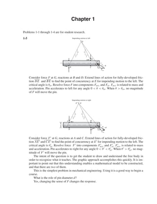
1. Chapter 1
Problems 1-1 through 1-4 are for student research.
1-5
D
B
G
F
Facc
A
Impending motion to left
E
1 1
f f
cr
C
Fcr
Consider force F at G, reactions at B and D. Extend lines of action for fully-developed fric-tion
DE and BE to find the point of concurrency at E for impending motion to the left. The
critical angle is θcr. Resolve force F into components Facc and Fcr. Facc is related to mass and
acceleration. Pin accelerates to left for any angle 0 θ θcr. When θ θcr, no magnitude
of F will move the pin.
D
B
G
F
Facc
A
E E
1 1
f f
C
d
Impending motion to right
Fcr
cr
Consider force F at G, reactions at A and C. Extend lines of action for fully-developed fric-tion
AE and CE to find the point of concurrency at E for impending motion to the left. The
cr. Resolve force F into components F
critical angle is θ
acc and F
cr. F
acc is related to mass
and acceleration. Pin accelerates to right for any angle 0 θ
θ
cr. When θ
θ
cr, no mag-nitude
of F will move the pin.
The intent of the question is to get the student to draw and understand the free body in
order to recognize what it teaches. The graphic approach accomplishes this quickly. It is im-portant
to point out that this understanding enables a mathematical model to be constructed,
and that there are two of them.
This is the simplest problem in mechanical engineering. Using it is a good way to begin a
course.
What is the role of pin diameter d?
Yes, changing the sense of F changes the response.

2. 2 Solutions Manual • Instructor’s Solution Manual to Accompany Mechanical Engineering Design
1-6
(a)
Fy = −F − f N cos θ + N sin θ = 0 (1)
Fx = f N sin θ + N cos θ − T
r
= 0
F = N(sin θ − f cos θ) Ans.
T = Nr( f sin θ + cos θ)
Combining
T = Fr
1 + f tan θ
tan θ − f
= KFr Ans. (2)
x
y
F
fN
N
T
r
(b) If T →∞detent self-locking tan θ − f = 0 ∴ θcr = tan−1 f Ans.
(Friction is fully developed.)
Check: If F = 10 lbf, f = 0.20, θ = 45◦, r = 2 in
N = 10
−0.20 cos 45◦ + sin 45◦
= 17.68 lbf
T
r
= 17.28(0.20 sin 45◦ + cos 45◦) = 15 lbf
f N = 0.20(17.28) = 3.54 lbf
θcr = tan−1 f = tan−1(0.20) = 11.31◦
11.31° θ 90°
1-7
(a) F = F0 + k(0) = F0
T1 = F0r Ans.
(b) When teeth are about to clear
F = F0 + kx2
From Prob. 1-6
T2 = Fr
f tan θ + 1
tan θ − f
T2 = r
(F0 + kx2)( f tan θ + 1)
tan θ − f
Ans.
1-8
Given, F = 10 + 2.5x lbf, r = 2 in, h = 0.2 in, θ = 60◦, f = 0.25, xi = 0, xf = 0.2
Fi = 10 lbf; Ff = 10 + 2.5(0.2) = 10.5 lbf Ans.

3. Chapter 1 3
From Eq. (1) of Prob. 1-6
N = F
− f cos θ + sin θ
Ni = 10
−0.25 cos 60◦ + sin 60◦
= 13.49 lbf Ans.
Nf = 10.5
10
13.49 = 14.17 lbf Ans.
From Eq. (2) of Prob. 1-6
K = 1 + f tan θ
tan θ − f
= 1 + 0.25 tan 60◦
tan 60◦ − 0.25
= 0.967 Ans.
Ti = 0.967(10)(2) = 19.33 lbf · in
Tf = 0.967(10.5)(2) = 20.31 lbf · in
1-9
(a) Point vehicles
Q = cars
hour
= v
x
= 42.1v − v2
0.324
Seek stationary point maximum
dQ
dv
= 0 = 42.1 − 2v
0.324
∴ v* = 21.05 mph
Q* = 42.1(21.05) − 21.052
0.324
= 1367.6 cars/h Ans.
(b)
Q = v
x + l
=
0.324
v(42.1) − v2
+ l
v
−1
Maximize Q with l = 10/5280 mi
v Q
22.18 1221.431
22.19 1221.433
22.20 1221.435 ←
22.21 1221.435
22.22 1221.434
% loss of throughput
1368 − 1221
1221
= 12% Ans.
x l2
l2
v
x
v

4. 4 Solutions Manual • Instructor’s Solution Manual to Accompany Mechanical Engineering Design
(c) % increase in speed
22.2 − 21.05
21.05
= 5.5%
Modest change in optimal speed Ans.
1-10 This and the following problem may be the student’s first experience with a figure of merit.
• Formulate fom to reflect larger figure of merit for larger merit.
• Use a maximization optimization algorithm. When one gets into computer implementa-tion
and answers are not known, minimizing instead of maximizing is the largest error
one can make.
FV = F1 sin θ − W = 0
FH = −F1 cos θ − F2 = 0
From which
F1 = W/sin θ
F2 = −W cos θ/sin θ
fom =−S=−¢γ (volume)
.=
−¢γ(l1A1 + l2A2)
A1 = F1
S
= W
S sin θ
, l2 = l1
cos θ
A2 =
F2
S
= W cos θ
S sin θ
fom = −¢γ
l2
cos θ
W
S sin θ
+ l2W cos θ
S sin θ
=
−¢γ Wl2
S
1 + cos2 θ
cos θ sin θ
Set leading constant to unity
◦ fom
0 −∞
20 −5.86
30 −4.04
40 −3.22
45 −3.00
50 −2.87
54.736 −2.828
60 −2.886
θ
θ* = 54.736◦ Ans.
fom* = −2.828
Alternative:
d
dθ
1 + cos2 θ
cos θ sin θ
= 0
And solve resulting tran-scendental
for θ*.
Check second derivative to see if a maximum, minimum, or point of inflection has been
found. Or, evaluate fom on either side of θ*.

5. Chapter 1 5
1-11
(a) x1 + x2 = X1 + e1 + X2 + e2
error = e = (x1 + x2) − (X1 + X2)
= e1 + e2 Ans.
(b) x1 − x2 = X1 + e1 − (X2 + e2)
e = (x1 − x2) − (X1 − X2) = e1 − e2 Ans.
(c) x1x2 = (X1 + e1)(X2 + e2)
e = x1x2 − X1X2 = X1e2 + X2e1 + e1e2
.=
X1e2 + X2e1 = X1X2
e1
X1
+ e2
X2
Ans.
(d)
x1
x2
= X1 + e1
X2 + e2
= X1
X2
1 + e1/X1
1 + e2/X2
1 + e2
X2
−1
.=
1 − e2
X2
and
1 + e1
X1
1 − e2
X2
.=
1 + e1
X1
− e2
X2
e = x1
x2
− X1
X2
.=
X1
X2
e1
X1
− e2
X2
Ans.
1-12
(a) x1 =
√
5 = 2.236 067 977 5
X1 = 2.23 3-correct digits
x2 =
√
6 = 2.449 487 742 78
X2 = 2.44 3-correct digits
x1 + x2 =
√
5 +
√
6 = 4.685 557 720 28
e1 = x1 − X1 =
√
5 − 2.23 = 0.006 067 977 5
e2 = x2 − X2 =
√
6 − 2.44 = 0.009 489 742 78
e = e1 + e2 =
√
5 − 2.23 +
√
6 − 2.44 = 0.015 557 720 28
Sum = x1 + x2 = X1 + X2 + e
= 2.23 + 2.44 + 0.015 557 720 28
= 4.685 557 720 28 (Checks) Ans.
(b) X1 = 2.24, X2 = 2.45
e1 =
√
5 − 2.24 = −0.003 932 022 50
e2 =
√
6 − 2.45 = −0.000 510 257 22
e = e1 + e2 = −0.004 442 279 72
Sum = X1 + X2 + e
= 2.24 + 2.45 + (−0.004 442 279 72)
= 4.685 557 720 28 Ans.

6. 6 Solutions Manual • Instructor’s Solution Manual to Accompany Mechanical Engineering Design
1-13
(a) σ = 20(6.89) = 137.8 MPa
(b) F = 350(4.45) = 1558 N = 1.558 kN
(c) M = 1200 lbf · in (0.113) = 135.6 N · m
(d) A = 2.4(645) = 1548 mm2
(e) I = 17.4 in4 (2.54)4 = 724.2 cm4
(f ) A = 3.6(1.610)2 = 9.332 km2
(g) E = 21(1000)(6.89) = 144.69(103) MPa = 144.7 GPa
(h) v = 45 mi/h (1.61) = 72.45 km/h
(i) V = 60 in3 (2.54)3 = 983.2 cm3 = 0.983 liter
1-14
(a) l = 1.5/0.305 = 4.918 ft = 59.02 in
(b) σ = 600/6.89 = 86.96 kpsi
(c) p = 160/6.89 = 23.22 psi
(d) Z = 1.84(105)/(25.4)3 = 11.23 in3
(e) w = 38.1/175 = 0.218 lbf/in
(f) δ = 0.05/25.4 = 0.00197 in
(g) v = 6.12/0.0051 = 1200 ft/min
(h) = 0.0021 in/in
(i) V =30/(0.254)3 = 1831 in3
1-15
(a) σ = 200
15.3
= 13.1MPa
(b) σ = 42(103)
6(10−2)2
= 70(106) N/m2 = 70 MPa
(c) y = 1200(800)3(10−3)3
3(207)(6.4)(109)(10−2)4
= 1.546(10−2) m = 15.5 mm
(d) θ = 1100(250)(10−3)
79.3(π/32)(25)4(109)(10−3)4
= 9.043(10−2) rad = 5.18◦
1-16
(a) σ = 600
20(6)
= 5 MPa
(b) I = 1
12
8(24)3 = 9216mm4
(c) I = π
64
324(10−1)4 = 5.147 cm4
(d) τ = 16(16)
π(253)(10−3)3
= 5.215(106) N/m2 = 5.215 MPa

7. Chapter 1 7
1-17
(a) τ = 120(103)
(π/4)(202)
= 382 MPa
(b) σ = 32(800)(800)(10−3)
π(32)3(10−3)3
= 198.9(106) N/m2 = 198.9MPa
(c) Z = π
32(36)
(364 − 264) = 3334 mm3
(d) k = (1.6)4 (79.3)(10−3)4(109)
8(19.2)3(32)(10−3)3
= 286.8 N/m