Introductory Mathematics for Earth Scientists

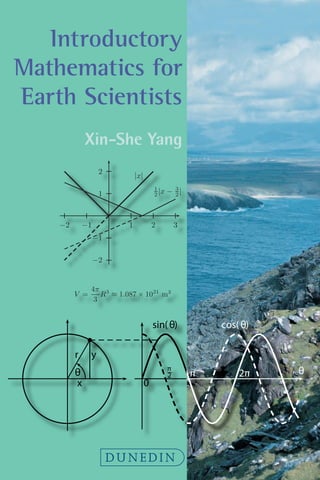
1. Introductory
Mathematics for
Earth Scientists
Xin-She Yang
DUNEDIN
0 1 2
0
10
x
Figure 1.3: The graph of the function y = f(x) = 4πx3
/3.
1.1.2 Quadratic Functions
A function is a quantity (say y) which varies with another independent
quantity x in a deterministic way. For example, the volume of a sphere
with a radius x is simply
y =
4π
3
x3
, (1.2)
which is an example of a cubic function. For any given value of x, there
is a unique corresponding value of y. By varying x smoothly, we can
vary y in such a manner so that the point (x, y) will trace out a curve
on the x−y plane (see Fig. 1.3). Thus, x is called independent variable,
and y is called the dependent variable or function. Sometimes, in order
to emphasize the relationship, we often use f(x) to express a general
function, showing that it is a function of x. This can also be written
as y = f(x).
Example 1.2: The average density of the Earth can be calculated by
ρ =
M�
V
,
where M� ≈ 5.979×1024
kg is the mass of the Earth, and V is the volume
of the Earth. Since the radius of the Earth is about R = 6.378 × 103
km
= 6.378 × 106
m, the volume is
V =
4π
3
R3
≈ 1.087 × 1021
m3
,
so the mean density is approximately
ρ =
5.979 × 1024
1.087 × 1021
≈ 5.502 × 103
kg/m3
= 5.502g/cm3
.
6 (by Yang X.-S.) 1. Preliminary Mathematics I
1 2 3
−1
−2
1
2
−1
−2
|x|
1
2 |x − 3
2 |
Figure 1.5: Graphs of modulus functions.
Two examples of modulus functions f(x) = |x| and f(x) = 1
2
|x− 3
2
|
are shown as solid lines in Fig. 1.5. The dashed lines corresponds to x
and 1
2 (x − 3
2 ) (without the modulus operator), respectively.
Example 1.3: The escape velocity of a satellite can be calculated as
follows: The kinetic energy of a moving object is
Ek =
1
2
mv2
,
where m is the mass of the object, and v is its velocity. The potential
energy due to the Earth’s gravitational force is
V = −
GMEm
r
,
where ME is the mass of the Earth, r is the radius of the Earth, and G is
the universal gravitational constant.
The total energy must be zero if the object is just able to escape the
Earth. We have
1 2 GMEm
y
x
θ
r
θ
sin(θ) cos( θ)
0
π
2 π 2π
y
x
θ
r
θ
sin(θ) cos( θ)
0
π
2 π 2π

2. Introductory Mathematics for Earth Scientists

3. By the same author and published by Dunedin Academic Press:
Mathematical Modelling for Earth Sciences (2008)
ISBN: 9781903765920

4. INTRODUCTORY
MATHEMATICS FOR
EARTH SCIENTISTS
Xin-She Yang
Department of Engineering, University of Cambridge
DUNEDIN

5. Published by
Dunedin Academic Press ltd
Hudson House
8 Albany Street
Edinburgh EH1 3QB
Scotland
www.dunedinacademicpress.co.uk
ISBN 978-1-906716-0-04
© 2009 Xin-She Yang
The right of Xin-She Yang to be identified as the author of this work has been asserted
by him in accordance with sections 77 and 78 of the Copyright, Designs and Patents
Act 1988.
All rights reserved.
No part of this publication may be reproduced or transmitted in any form or by any
means or stored in any retrieval system of any nature without prior written permission,
except for fair dealing under the Copyright, Designs and Patents Act 1988 or in
accordance with the terms of a licence issued by the Copyright Licensing Society in
respect of photocopying or reprographic reproduction. Full acknowledgment as to
author, publisher and source must be given. Application for permission for any other
use of copyright material should be made in writing to the publisher.
British Library Cataloguing in Publication data
A catalogue record for this book is available from the British Library
While all reasonable attempts have been made to ensure the accuracy of information
contained in this publication it is intended for prudent and careful professional and
student use and no liability will be accepted by the author or publishers for any loss,
damage or injury caused by any errors or omissions herein. This disclaimer does not
effect any statutory rights.
Printed in the United Kingdom by Cpod, Trowbridge, Wiltshire
Printed on paper from sustainable resources
© Bob Deacon 2007
Apart from any fair dealing for the purposes of research
or private study, or criticism or review, as permitted
under the Copyright, Designs and Patents Act, 1988, this
publication may be reproduced, stored or transmitted
in any form, or by any means, only with the prior
permission in writing of the publishers, or in the case of
reprographic reproduction, in accordance with the terms
of licences issued by the Copyright Licensing Agency.
Enquiries concerning reproduction outside those terms
should be sent to the publishers.
SAGE Publications Ltd
1 Oliver’s Yard
55 City Road
London EC1Y 1SP
SAGE Publications Inc.
2455 Teller Road
Thousand Oaks, California 91320
SAGE Publications India Pvt Ltd
Mathura Road, New Delhi 110 044
India
SAGE Publications Asia-Pacific Pte Ltd
33 Pekin Street #02-01
Far East Square
Singapore 048763
British Library Cataloguing in Publication data
A catalogue record for this book is available
from the British Library
ISBN 978-1-4129-0762-0 (pbk)
Library of Congress Control Number: 2006931639
Typeset by C&M Digitals (P) Ltd., Chennai, India
Printed on paper from sustainable resources
Printed and bound in Great Britain by Cpod, Trowbridge, Wiltshire
ISBN 978-1-4129-0761-3 (hbk)
First published 2007
Reprinted 2009
B 1/I 1 Mohan Cooperative Industrial Area

6. Contents
Preface v
1 Preliminary Mathematics I 1
1.1 Functions . . . . . . . . . . . . . . . . . . . . . . . . . . 2
1.1.1 Real Numbers . . . . . . . . . . . . . . . . . . . . 2
1.1.2 Functions . . . . . . . . . . . . . . . . . . . . . . 3
1.2 Equations . . . . . . . . . . . . . . . . . . . . . . . . . . 10
1.3 Index Notation . . . . . . . . . . . . . . . . . . . . . . . 13
1.3.1 Notations of Indices . . . . . . . . . . . . . . . . 13
1.3.2 Graphs of Functions . . . . . . . . . . . . . . . . 16
1.4 Applications . . . . . . . . . . . . . . . . . . . . . . . . . 16
1.4.1 Greenhouse Effect . . . . . . . . . . . . . . . . . 17
1.4.2 Glacier Flow . . . . . . . . . . . . . . . . . . . . 18
1.4.3 Airy Isostasy . . . . . . . . . . . . . . . . . . . . 19
1.4.4 Size of an Impact Crater . . . . . . . . . . . . . . 20
2 Preliminary Mathematics II 21
2.1 Polynomials . . . . . . . . . . . . . . . . . . . . . . . . . 21
2.2 Roots . . . . . . . . . . . . . . . . . . . . . . . . . . . . 22
2.3 Descartes’ Theorem . . . . . . . . . . . . . . . . . . . . 25
2.4 Applications . . . . . . . . . . . . . . . . . . . . . . . . . 27
2.4.1 Stokes’ Flow . . . . . . . . . . . . . . . . . . . . 27
2.4.2 Velocity of a Raindrop . . . . . . . . . . . . . . . 29
3 Binomial Theorem and Sequences 31
3.1 The Binomial Theorem . . . . . . . . . . . . . . . . . . 31
3.1.1 Factorials . . . . . . . . . . . . . . . . . . . . . . 32
3.1.2 Binomial Theorem and Pascal’s Triangle . . . . . 33
3.2 Sequences . . . . . . . . . . . . . . . . . . . . . . . . . . 34
3.2.1 Fibonacci Sequence . . . . . . . . . . . . . . . . . 36
3.2.2 Sum of a Series . . . . . . . . . . . . . . . . . . . 38
3.2.3 Infinite Series . . . . . . . . . . . . . . . . . . . . 41
3.3 Exponentials and Logarithms . . . . . . . . . . . . . . . 42
3.4 Applications . . . . . . . . . . . . . . . . . . . . . . . . . 44
i
v
ix

7. vi Contents
ii CONTENTS
3.4.1 Carbon Dioxide . . . . . . . . . . . . . . . . . . . 44
3.4.2 Folds . . . . . . . . . . . . . . . . . . . . . . . . . 45
3.4.3 Gutenberg-Richter Law . . . . . . . . . . . . . . 45
3.4.4 Distribution of Near-Earth Objects . . . . . . . . 47
4 Trigonometry and Spherical Trigonometry 49
4.1 Plane Trigonometry . . . . . . . . . . . . . . . . . . . . 49
4.1.1 Trigonometrical Functions . . . . . . . . . . . . . 49
4.1.2 Sine Rule . . . . . . . . . . . . . . . . . . . . . . 57
4.1.3 Cosine Rule . . . . . . . . . . . . . . . . . . . . . 58
4.2 Spherical Trigonometry . . . . . . . . . . . . . . . . . . 59
4.3 Applications . . . . . . . . . . . . . . . . . . . . . . . . . 61
4.3.1 Travel-Time Curves of Seismic Waves . . . . . . 61
4.3.2 Great-Circle Distance . . . . . . . . . . . . . . . 63
4.3.3 Bubbles and Surface Tension . . . . . . . . . . . 64
5 Complex Numbers 67
5.1 Complex Numbers . . . . . . . . . . . . . . . . . . . . . 67
5.1.1 Imaginary Numbers . . . . . . . . . . . . . . . . 67
5.1.2 Polar Form . . . . . . . . . . . . . . . . . . . . . 70
5.2 Hyperbolic Functions . . . . . . . . . . . . . . . . . . . . 72
5.2.1 Hyperbolic Sine and Cosine . . . . . . . . . . . . 72
5.2.2 Hyperbolic Identities . . . . . . . . . . . . . . . . 73
5.2.3 Inverse Hyperbolic Functions . . . . . . . . . . . 74
5.3 Water Waves . . . . . . . . . . . . . . . . . . . . . . . . 75
6 Differentiation 77
6.1 Gradient . . . . . . . . . . . . . . . . . . . . . . . . . . . 77
6.2 Differentiation Rules . . . . . . . . . . . . . . . . . . . . 82
6.3 Partial Derivatives . . . . . . . . . . . . . . . . . . . . . 85
6.4 Maxima or Minima . . . . . . . . . . . . . . . . . . . . . 87
6.5 Series Expansions . . . . . . . . . . . . . . . . . . . . . . 89
6.6 Applications . . . . . . . . . . . . . . . . . . . . . . . . . 91
6.6.1 Free-Air Gravity . . . . . . . . . . . . . . . . . . 91
6.6.2 Mantle Convection . . . . . . . . . . . . . . . . . 92
7 Integration 95
7.1 Integration . . . . . . . . . . . . . . . . . . . . . . . . . 95
7.2 Integration by Parts . . . . . . . . . . . . . . . . . . . . 100
7.3 Integration by Substitution . . . . . . . . . . . . . . . . 103
7.4 Bouguer Gravity . . . . . . . . . . . . . . . . . . . . . . 105

8. Contents vii
CONTENTS iii
8 Fourier Transforms 107
8.1 Fourier Series . . . . . . . . . . . . . . . . . . . . . . . . 107
8.2 Fourier Transforms . . . . . . . . . . . . . . . . . . . . . 111
8.3 DFT and FFT . . . . . . . . . . . . . . . . . . . . . . . 112
8.4 Milankovitch Cycles . . . . . . . . . . . . . . . . . . . . 114
9 Vectors 117
9.1 Vector Algebra . . . . . . . . . . . . . . . . . . . . . . . 117
9.1.1 Vectors . . . . . . . . . . . . . . . . . . . . . . . 117
9.1.2 Product of Vectors . . . . . . . . . . . . . . . . . 122
9.2 Gradient and Laplace Operators . . . . . . . . . . . . . 126
9.3 Applications . . . . . . . . . . . . . . . . . . . . . . . . . 129
9.3.1 Mohr-Coulomb Criterion . . . . . . . . . . . . . 129
9.3.2 Thrust Faults . . . . . . . . . . . . . . . . . . . . 131
9.3.3 Electrical Method in Prospecting . . . . . . . . . 132
10 Matrix Algebra 135
10.1 Matrices . . . . . . . . . . . . . . . . . . . . . . . . . . . 135
10.2 Transformation and Inverse . . . . . . . . . . . . . . . . 138
10.3 Eigenvalues and Eigenvectors . . . . . . . . . . . . . . . 144
10.4 Harmonic Motion . . . . . . . . . . . . . . . . . . . . . . 147
11 Ordinary Differential Equations 149
11.1 Differential Equations . . . . . . . . . . . . . . . . . . . 149
11.2 First-Order Equations . . . . . . . . . . . . . . . . . . . 150
11.3 Second-Order Equations . . . . . . . . . . . . . . . . . . 156
11.4 Higher-Order ODEs . . . . . . . . . . . . . . . . . . . . 161
11.5 Applications . . . . . . . . . . . . . . . . . . . . . . . . . 163
11.5.1 Climate Changes . . . . . . . . . . . . . . . . . . 163
11.5.2 Flexural Deflection of Lithosphere . . . . . . . . 165
11.5.3 Glacial Isostatic Adjustment . . . . . . . . . . . 168
12 Partial Differential Equations 171
12.1 Introduction . . . . . . . . . . . . . . . . . . . . . . . . . 171
12.2 Classic Equations . . . . . . . . . . . . . . . . . . . . . . 172
12.3 Heat Conduction . . . . . . . . . . . . . . . . . . . . . . 173
12.4 Cooling of the Lithosphere . . . . . . . . . . . . . . . . . 176
13 Geostatistics 179
13.1 Random Variables . . . . . . . . . . . . . . . . . . . . . 179
13.1.1 Probability . . . . . . . . . . . . . . . . . . . . . 179
13.1.2 Mean and Variance . . . . . . . . . . . . . . . . . 181
13.2 Sample Mean and Variance . . . . . . . . . . . . . . . . 183
13.3 Propagation of Errors . . . . . . . . . . . . . . . . . . . 184
13.4 Linear Regression . . . . . . . . . . . . . . . . . . . . . . 188
13.5 Correlation Coefficient . . . . . . . . . . . . . . . . . . . 191

9. viii Contents
iv CONTENTS
13.6 Brownian Motion . . . . . . . . . . . . . . . . . . . . . . 192
14 Numerical Methods 195
14.1 Finding the roots . . . . . . . . . . . . . . . . . . . . . . 195
14.2 Newton-Raphson Method . . . . . . . . . . . . . . . . . 196
14.3 Numerical Integration . . . . . . . . . . . . . . . . . . . 198
14.4 Numerical Solutions of ODEs . . . . . . . . . . . . . . . 201
14.4.1 Euler Scheme . . . . . . . . . . . . . . . . . . . . 202
14.4.2 Runge-Kutta Method . . . . . . . . . . . . . . . 203
Bibliography 207
A Glossary 211
B Mathematical Formulae 217
Epilogue 221
Index 223

10. Preface v
Preface
Any quantitative analysis in earth sciences requires mathematical anal-
ysis to a certain degree, and many mathematical methods are essential
to the modelling and analysis of the geological, geophysical and environ-
mental processes widely studied in earth sciences. In response to such
needs in modern earth sciences, the author wrote a book on Mathemat-
ical Modelling for Earth Sciences published by Dunedin Academic in
2008 with the intention of filling the gaps between mathematical mod-
elling and its practical applications in earth sciences. The responses of
enthusiastic readers and professional reviews of the book in scientific
journals such as Geoscientist and Journal of Sedimentary Research are
very encouraging and positive. We realised that Mathematical Mod-
elling for Earth Sciences is most suitable for the third and final year
undergraduates with more mathematical training, graduates and re-
searchers. As we understand from various surveys and interactions
with earth scientists, the mathematical training of new undergraduates
often begins at the secondary school or GCSE level. This may pose
substantial challenge in teaching a wide range of mathematical skills
along with the specialised subjects in earth sciences. This present book
is an attempt to bridge the gaps between secondary mathematics and
mathematical skills at university level.
This introductory book strives to provide a comprehensive intro-
duction to the fundamental mathematics that all earth scientists need.
The book is self-contained and provides an essential toolkit of basic
mathematics for earth scientists assuming no more than a standard
secondary school level as its starting point.
The topics of earth sciences are vast and multidisciplinary, and con-
sequently the mathematical tools required by students are diverse and
complex. Thus, we have to strike a fine balance between coverage and
detail. Topics have been selected to provide a concise but comprehen-
sive introductory coverage of all the major and popular mathematical
methods. The book offers a ‘theorem-free’ approach with an emphasis
on practicality. With more than a hundred step-by-step worked ex-
amples and dozens of well-selected illustrative case studies, the book is
specially suitable for non-mathematicians and geoscientists. The topics
include binomial theorem, index notations, polynomials, sequences and
series, trigonometry, spherical trigonometry, complex numbers, vectors
and matrices, ordinary differential equations, partial differential equa-
tions, Fourier transforms, numerical methods and geostatistics.
Mathematics is an exact science; however, the ability and skills to
be able to do estimations are also crucially important in many appli-
cations in earth sciences. Many processes in earth sciences are coupled
together and it is difficult, even impossible in most cases, to get the
exact solutions or answers to a problem of interest. In this case, some
ix

11. vi Preface
estimations using simple formulae, rather than complex mathematics,
often provide more insight to the underlying mechanism and processes.
To get the right magnitudes or orders of some quantities by simple es-
timation is an art that needs development by practice. For example,
we know the tectonic plate drifts at a speed of about a few centimetres
per year, this can be obtained by using the age difference and distances
among the Hawaii Islands. The magnitude is a few centimetres per
year, not millimetres per year or kilometres per year. If we want a
higher accuracy, we have to use complex partial differential equations,
the actual geometry of the plate, the detailed knowledge of the Earth’s
interior, the mantle convection mechanism, and many other inputs. We
also have to make sure that we have the right mathematical models and
the appropriate solution techniques both analytically and numerically.
In the end, we may produce seemingly more accurate solutions. How-
ever, we may still not believe the results as there are so many factors
by which they can be affected. In this case, a simple estimate is very
useful and provides a good basis to build more complex or realistic
models. In this book, we will provide dozens of examples to guide
you in using basic mathematics to actually model important processes
and evaluate the right orders or magnitudes of solutions. The case
studies include the Airy isostasy, the flexural deflection of a tectonic
plate, greenhouse effect, Brownian motion, sedimentation and Stokes’
flow, free-air and Bouguer gravity, heat conduction, the cooling of the
lithosphere, earthquakes and many others.
Introductory Mathematics for Earth Scientists introduces a wide
range of fundamental and yet widely-used mathematical methods. It
is designed for use by undergraduates, though postgraduate students
will also find it a helpful reference and aide-memoire.
In writing the book, I sent more than 100 questionnaires to many
university professors, lecturers and students at various universities in-
cluding Oxford, Cambridge, MIT, Imperial, Princeton, Caltech, Col-
orado, Cornell, Leeds, and Newcastle (Australia). Their valuable com-
ments to my questionnaires concerning the essential mathematical skills
of earth scientists, selection of mathematical topics, and their relevance
to applications have been incorporated in the book. In addition, I have
received a variety of help from my colleagues and students. Special
thanks to my students at Cambridge University: Joanne Perry, Edward
Flower, Alisdair McClymont, Omar Kadhim, Mi Liu, Maxine Jordan,
Priyanka De Souza, Michelle Stewart, Shu Yang, Young Z. L. Yang,
and Qi Zhang.
Last but not least, I thank my wife and son for their help.
Xin-She Yang
Cambridge 2009
x PREFACE

12. Chapter 1
Preliminary
Mathematics I
The basic requirement for this book is a good understanding of sec-
ondary mathematics, about the GCSE1
level mathematics. All the fun-
damental mathematics will be gradually introduced in a self-contained
style with plenty of worked examples to aid the understanding of es-
sential concepts.
We are concerned mainly with the introduction to important math-
ematical techniques; however, we have to deal with physical quantities
with units. We will mainly use SI units throughout this book. For ex-
ample, we use kg/m3
for density, metrer (m) for length, seconds (s) for
time, m/s for velocity, m/s2
for acceleration, Pascals (Pa) for pressure
and stress, Pascal-seconds (Pa s) for viscosity, and Kelvin (K) or de-
gree Celsius (◦
C) for temperature. The unit of geological time is often
expressed in terms of million years (Ma), and occasionally, years (yr
or a). As for the latter, yr becomes a popular usage, though a was a
formal usage. Therefore, we will use yr for simplicity.
The applications of mathematics in earth sciences are as diverse as
the subject itself. For a particular problem, we often have to use many
different mathematical techniques, and more often their combinations,
to obtain a good solution to the problem of interest. For example,
in order to obtain the deflection of the lithosphere under a given load
as discussed in later chapters, we have to use almost all the impor-
tant techniques introduced in this book, including basic mathematics,
trigonometry, complex numbers, and differential equations.
On the other hand, a good mathematical technique can be applied
to a wide range of problems. For example, simple manipulations of
1General Certificate of Secondary Education, achieved usually at age 16 in the
UK by a vast majority of students in any subject before proceeding to A level
studies and/or undergraduate studies.
1

13. 2 Chapter 1. Preliminary Mathematics I
0 1 2 3 4
−1
−2
−3
r
A
r
B
Figure 1.1: Real numbers and their representations (as points
or locations) on the number line.
index forms and basic algebraic equations can be applied in studying
the greenhouse effect, glacier flow, isostasy and the estimation of the
size of an impacting crater, as will be demonstrated later in this chapter.
1.1 Functions
1.1.1 Real Numbers
From basic mathematics, we know that whole numbers such as −5, 0
and 2 are integers, while the positive integers such as 1, 2, 3, ... are often
called natural numbers. The ratio of any two non-zero integers p and
q in general is a fraction p/q where q 6= 0. For example, 1
2 , −4
3 and 22
7
are fractions. If p < q, the fraction is called a proper fraction. All the
integers and fractions make up the rational numbers.
Numbers such as
√
2 and π are called irrational numbers because
they cannot be expressed in terms of a fraction. Rational numbers and
irrational numbers together make up the real numbers. In mathematics,
all the real numbers are often denoted by <, and any real number
corresponds to a unique point or location in the number line (see Fig.
1.1). For example, 3/2 corresponds to point A and −
√
2 corresponds
to point B.
In a plane, any point can be located by a pair of two real numbers
(x, y), which are called Cartesian coordinates (see Fig. 1.2). For ease of
reference to a location or different part on the plane, we conventionally
divide the coordinate system into four quadrants. From the first quad-
rant with (x > 0, y > 0) in an anti-clockwise manner, we consecutively
call them the second, third and fourth quadrants as shown in Fig. 1.2.
Such representation makes it straightforward to calculate the distance
d, often called Cartesian distance, between any two points A(xi, yi) and
B(xj, yj). The distance is the line segment AB, which can be obtained
by the Pythagoras’s theorem for the right-angled triangle ABC. We
have
d =
q
(xi − xj)2 + (yi − yj)2 ≥ 0. (1.1)

14. 1.1 Functions 3
1 2
−1
−2
1
−1
s
A(1.25, 1.7)
s
B(−2, 0.5)
C
x
y
x
y
First quadrant
(x> 0, y> 0)
Second quadrant
(x< 0, y> 0)
Third quadrant
(x< 0, y< 0)
Fourth quadrant
(x> 0, y< 0)
Figure 1.2: Cartesian coordinates and the four quadrants.
Example 1.1: For example, the point A(1.25, 1.7) lies in the first
quadrant, while point B(−2, 0.5) lies in the second quadrant. The distance
between A and B is the length along the straight line connecting A and
B, and we have
d =
p
[1.25 − (−2)]2 + (1.7 − 0.5)2 =
√
12.0025 ≈ 3.4645,
which should have the same unit as the coordinates themselves. Here the
sign ‘≈’ means ‘is approximately equal to’.
1.1.2 Functions
A function is a quantity (say y) which varies with another independent
quantity x in a deterministic way.
For example, the permeability of a porous material is closely related
to its grain size by a quadratic function
K = CD2
, (1.2)
which is the Hazen’s empirical relationship between permeability and
grain size D. In generally, the larger the grain size, the larger the pores
or voids, and thus the higher the permeability. Let D ≈ D10 be Hazen’s
effective size or diameter (in cm). Then, C ≈ 100 if K is in the unit of
cm2
, while C ≈ 0.01 if K has a unit of m2
. For example, for very fine
sand and fine sand, D ≈ 0.0625 to 0.5 mm (or 1/16 to 1/2 mm). Using
D = 0.1 mm = 0.01 cm, we have
K ≈ 0.01 × (0.01)2
= 10−6
m2
. (1.3)
Furthermore, the volume y of a sphere with a radius x is simply
y =
4π
3
x3
, (1.4)

15. 4 Chapter 1. Preliminary Mathematics I
0 1 2
0
10
20
x
y
Figure 1.3: The graph of the function y = f(x) = 4πx3
/3.
which is an example of a cubic function. For any given value of x, there
is a unique corresponding value of y. By varying x smoothly, we can
vary y in such a manner that the point (x, y) will trace out a curve
on the x − y plane (see Fig. 1.3). Thus, x is called the independent
variable, and y is called the dependent variable or function. Sometimes,
in order to emphasize the relationship, we use f(x) to express a general
function, showing that it is a function of x. This can also be written
as y = f(x).
Example 1.2: The average density of the Earth can be calculated by
ρ = M /V, where M ≈ 5.979 × 1024
kg is the mass of the Earth, and
V is the volume of the Earth. Since the radius of the Earth is about
R = 6.378 × 103
km = 6.378 × 106
m, the volume is
V =
4π
3
R3
≈ 1.087 × 1021
m3
,
so the mean density is approximately
ρ =
5.979 × 1024
1.087 × 1021
≈ 5.502 × 103
kg/m3
= 5.502 g/cm3
.
This is much higher than the density (typically 2.6 g/cm3
) of rocks near
the Earth’s surface, which implies that the density of the Earth’s interior
should be much higher, hence may be a very dense core.
For any real number x, there is a corresponding unique value y =
f(x) = 4πx3
/3, and although the negative volume is meaningless phys-
ically, it is valid mathematically. This relationship is a one-to-one map-
ping from x to y. In mathematics, when we say x is a real number, we
often write x ∈ <. Here < means the set of all real numbers, and ∈
stands for ‘is a member of’ or ‘belongs to’. Thus, x ∈ < is equivalent to
saying that x is a real number or a member of the set of real numbers.
The domain of a function is the set of numbers x for which the
function f(x) is defined validly. If a function is defined over a range
a ≤ x ≤ b, we say its domain is [a, b] which is called a closed interval.

16. 1.1 Functions 5
s
(0, c)
s
P(x, y)
gradient k
intercept
x
y
s
(x2, y2)
s
(x1, y1)
Figure 1.4: The equation y = kx + c and a line through two
points.
If a and b are not included, we have a < x < b which is denoted as
(a, b), and we call this interval an open interval. If b is included while
a is not, we have a < x ≤ b, and we often write this half-open and
half-closed interval as (a, b]. Thus, the domain of function f(x) = x2
is
the set of all real numbers < which is also written
−∞ < x < +∞. (1.5)
Here ∞ denotes infinity. The values that a function can take for a
given domain is called the range of the function. Thus, the range of
y = f(x) = x2
is 0 ≤ y < ∞ or [0, ∞).
Sometimes, it is more convenient to write a function in a concise
mathematical language, and we write
f : x 7→
1
2
x2
− 15, x ∈ <, (1.6)
which is called a mapping. This means that f(x) is a function of x and
this function will turn any real number x (input) in the domain into
another number (output) 1
2 x2
− 15.
The simplest general function is probably the linear function
y = kx + c, (1.7)
where k and c are real constants. For any given values of k and c, this
will usually lead to a straight line if we plot values y versus x on a
Cartesian coordinate system. In this case, k is the gradient of the line
and c is the intercept (see Fig. 1.4).
For any two different points A(x1, y1) and B(x2, y2), we can always
draw a straight line. Its gradient can be calculated by
k =
y2 − y1
x2 − x1
, (x1 6= x2). (1.8)
For any point P(x, y), the equation for the straight line becomes
y − y1
x − x1
= k =
y2 − y1
x2 − x1
. (1.9)

17. 6 Chapter 1. Preliminary Mathematics I
p
z
h
Figure 1.5: Pressure variations along the wall of a dam.
This is
y = y1 +
(y2 − y1)
(x2 − x1)
(x − x1) =
(y2 − y1)
(x2 − x1)
x + [y1 −
(y2 − y1)
(x2 − x1)
x1], (1.10)
which gives the intercept
c = y1 −
(y2 − y1)
(x2 − x1)
x1. (1.11)
In a special case y1 = y2 while x1 6= x2, we have k = 0. The line
becomes horizontal, and the equation simply becomes y = y1 which
does not depend on x as x does not appear in the equation.
In another special case, x1 = x2, k is very large or approaching
infinity, which we write as k → ∞. It becomes a vertical line. Any
small change in x will lead to an infinite change in y. For example,
if we have x1 = x2 = 2, we have a vertical line through x = 2, and
we simply write the equation as x = 2, and y does not appear in the
equation in this case.
Example 1.3: The water pressure p in a dam varies with depth z
p(z) = ρgz,
where ρ is the density of water, and g is the acceleration due to gravity.
The linear increase of pressure requires the dam thickness to increase with
depth so as to balance the pressure by shear strength of the dam (see Fig.
1.5). As the pressure is a linear function of z, the average pressure p̄ can
be calculated by
p̄ =
p(0) + p(h)
2
=
0 + ρgh
2
=
ρgh
2
.
A special function is the modulus function |x| which is defined by
|x| =
x if x ≥ 0,
−x if x 0.
(1.12)

18. 1.1 Functions 7
1 2 3
−1
−2
1
2
−1
−2
|x|
1
2 |x − 3
2 |
Figure 1.6: Graphs of modulus functions.
That is to say, |x| is always non-negative. For example, |5| = 5 and
| − 5| = 5.
The modulus function has the following properties
|a × b| = |a| × |b|, a, b ∈ , (1.13)
which means that |a2
| = |a|2
= a2
≥ 0 for any a ∈ . Similarly, for
any real numbers a and b 6= 0, we have
|
a
b
| =
|a|
|b|
. (1.14)
But for addition in general, we have |a + b| 6= |a| + |b|. In fact, there is
an equality in this case: |a + b| ≤ |a| + |b|, and we will discuss this in
detail in the vector analysis in later chapters.
Two examples of modulus functions f(x) = |x| and f(x) = 1
2 |x− 3
2 |
are shown as solid lines in Fig. 1.6. The dashed lines correspond to x
and 1
2 (x − 3
2 ) (without the modulus operator), respectively.
As an example, we now try to calculate the time taken for an object
to fall freely from a height of h to the ground. If we assume the object
is released with a zero velocity at h, we know from the basic physics
that the distance h it travels is
h =
1
2
gt2
, (1.15)
where t is the time taken, and g = 9.8 m/s2
is the acceleration due to
gravity. Now we have
t =
s
2h
g
. (1.16)
The velocity just before it hits the ground is v = gt or
v =
p
2gh. (1.17)

19. 8 Chapter 1. Preliminary Mathematics I
For example, the time taken for an object to fall from h = 20 m to
the ground is about t =
p
2 × 20/9.8 ≈ 2 seconds. The velocity it
approaches the ground is v ≈
√
2 × 9.8 × 20 ≈ 19.8 m/s.
Example 1.4: The escape velocity of a satellite can be calculated as
follows: The kinetic energy of a moving object is
Ek =
1
2
mv2
,
where m is the mass of the satelite, and v is its velocity. The potential
energy due to the Earth’s gravitational force is
V = −
GMEm
r
,
where ME is the mass of the Earth, r is the radius of the Earth, and G is
the universal gravitational constant.
The total energy must be zero if the object is just able to escape the
Earth. We have
Ek + V =
1
2
mv2
−
GMEm
r
= 0.
This means that
v =
r
2GME
r
.
Since the gravity g on the Earth surface is
g =
GMe
r2
,
we have
v =
p
2gr.
Using the values of g = 9.8 m/s2
, and r = 6370 km= 6.4 × 106
m, we
have
v =
p
2 × 9.8 × 6.4 × 106 ≈ 11170 m/s = 11.17 km/s.
Interestingly, the escape velocity is independent of the mass of the object.
Quadratic functions are widely used in many applications. In gen-
eral, a quadratic function y = f(x) can be written as
f(x) = ax2
+ bx + c, (1.18)
where the coefficients a, b and c are real numbers. Here we can assume
a 6= 0. If a = 0, it reduces to the case of linear functions that we have

20. 1.1 Functions 9
1 2
−1
1
2
−1
a 0
s
s
x
y
y=x2
−x−1
1
−1
1
2
−1
a 0
)
x
y
y=−2x2
−x+ 2
Figure 1.7: Graphs of quadratic functions.
discussed earlier. Two examples of quadratic functions are shown in
Fig. 1.7 where both a 0 and a 0 are shown, respectively.
Depending on the combination of the values of a, b, and c, the curve
may cross the x-axis twice, once (just touch), and not at all. The points
at which the curve crosses the x-axis are the roots of
f(x) = ax2
+ bx + c = 0. (1.19)
As we can assume a 6= 0, we have
x2
+
b
a
x +
c
a
= 0. (1.20)
Of course, we can use factorisation to find the solution in many cases.
For example, we can factorise x2
− 5x + 6 = 0 as
x2
− 5x + 6 = (x − 2)(x − 3) = 0, (1.21)
and the solution is thus either (x−2) = 0 or (x−3) = 0. That is x = 2
or x = 3. However, sometimes it is difficult (or even impossible) to
factorise even seemingly simple expressions such as x2
− x − 1. In this
case, it might be better to address the quadratic equation in a generic
manner using the so-called complete-square method.
Completing the square of the expression can be used to solve this
equation, and we have
x2
+
b
a
x +
c
a
= (x +
b
2a
)2
−
b2
4a2
+
c
a
= (x +
b
2a
)2
−
(b2
− 4ac)
4a2
= 0, (1.22)
which leads to
(x +
b
2a
)2
=
(b2
− 4ac)
4a2
. (1.23)

21. 10 Chapter 1. Preliminary Mathematics I
Taking the square root of the above equation, we have either
x +
b
2a
= +
r
b2 − 4ac
4a2
, or x +
b
2a
= −
r
b2 − 4ac
4a2
. (1.24)
Using
√
4a2 = +2a or −2a, we have
x = −
b
2a
±
√
b2 − 4ac
2a
=
−b ±
√
b2 − 4ac
2a
. (1.25)
In some books, the expression b2
− 4ac is often denoted by ∆. That is
∆ = b2
−4ac. If ∆ = b2
−4ac 0, there is no solution which corresponds
to the case where the curve does not cross the x-axis at all. In the
special case of b2
− 4ac = 0, we have a single solution x = −b/(2a),
which corresponds to the case where the curve just touches the x-axis.
In general, if b2
− 4ac 0, we have two distinct real roots. Let us look
at an example.
Example 1.5: For the quadratic function f(x) = x2
− x − 1, we have
a = 1, b = −1 and c = −1. Since
∆ = b2
− 4ac = (−1)2
− 4 × 1 × (−1) = 5 0,
it has two different real roots. We have
x1,2 =
−(−1) ±
√
∆
2
=
1 ±
√
5
2
.
So the two roots are (1−
√
5)/2 and (1+
√
5)/2 which are marked as solid
circles on the graph in Fig. 1.7.
Of course, many expressions involve higher-order terms such as x5
−
2x3
− 4x2
+ 1. In this case, we are dealing with polynomials which use
the notation of indices and manipulations of equations extensively.
1.2 Equations
When we discussed the quadratic function f(x) earlier, we have to find
where it crosses the x-axis. In this case, we have to solve the quadratic
equation ax2
+ bx + c = 0. In general, an equation is a mathematical
statement that is written in terms of symbols and an equal sign ‘=’.
All the terms on the left of ‘=’ are collectively called the left-hand side
(LHS), while those on the right of ‘=’ are called the right-hand side
(RHS). For example, x2
+ 2x − 3 = 0 is a quadratic equation with its
left-hand side being x2
+ 2x − 3 and right-hand side being 0.
An equation has the following properties: 1) any quantity can be
added to, subtracted from or multiplied by both sides of the equation;

22. 1.2 Equations 11
2) A non-zero quantity can divide both sides; and 3) any function
such as power and surds can be applied to both sides equally. After
such manipulations, an equation may be converted into a completely
different equation, though you can obtain the original equation if you
can carefully reverse the above procedure, though special care is needed
in some cases.
The idea of these manipulations is to transform the equation to a
more simple form whose solution can be found easily.
Example 1.6: For example, from equation
x2
+ 2x − 3 = 0, (1.26)
we can add the same term 4 to both sides, and we have
x2
+ 2x − 3 + 4 = 0 + 4, or x2
+ 2x + 1 = 4. (1.27)
Since (x + 1)2
= x2
+ 2x + 1, we get
(x + 1)2
= 4. (1.28)
We can take the square root of both sides, we have
p
(x + 1)2 = x + 1 = ±
√
4 = ±2. (1.29)
Here we have to keep ± as the square root of 4 can be either +2 or −2
(otherwise, we just find one root). Now we subtract +1 from (or add −1
to) both sides, we have
x +1 − 1
| {z }
sum=0
= ±2 − 1, (1.30)
which leads to
x + 0 = ±2 − 1, or x = ±2 − 1. (1.31)
This is equivalent to moving the term +1 on the left to the right and
changing its sign so that it becomes −1. Now we have two solutions
x = +2 − 1 = +1 and x = −2 − 1 = −3.
The same mathematical operations can also be applied to a system
of equations. In order to solve two simultaneous equations for the
unknowns x and y
5x +y = −7
−4x −2y = 2
, (1.32)
we first multiply both sides of the first equation by 2, we have
2 × (5x + y) = 2 × (−7), (1.33)

23. 12 Chapter 1. Preliminary Mathematics I
and we get
10x + 2y = −14. (1.34)
Now we add this equation (thinking of the same quantity on both sides)
to the second equation of the system. We have
10x +2y = −14
−4x −2y = 2
6x +0 = −12.
(1.35)
This means that
6x = −12, or x =
−12
6
= −2. (1.36)
Now substitute this solution x = −2 into one of the equations (say, the
first); we have
5 × (−2) + y = −7, (1.37)
or
−10 + y = −7. (1.38)
This simply leads to
y = −7 + 10 = 3. (1.39)
Now let us look at another example.
Example 1.7: The conversion from Fahrenheit F to Celsius C is given
by
C =
5
9
(F − 32).
Conversely, from Celsius to Fahrenheit, we have
F =
9C
5
+ 32.
So the melting point of ice C = 0◦
C is equivalent to F = 9×0
5 +32 = 32◦
F,
while the boiling point of water C = 100◦
C becomes 9 × 100/5 + 32 =
212◦
F.
We can see that these two temperature scales are very different. How-
ever, there is a single temperature at which these two coincide. Let us
now try to determine this temperature. We have C = F, that is
5
9
(F − 32) =
9C
5
+ 32 =
9F
5
+ 32,
which becomes
(
5
9
−
9
5
)F = 32 +
160
9
,
or
−
56
45
F =
448
9
.
The solution is simply F = C = −40. This means that −40◦
F and −40◦
C
represent the same temperature on both scales.

24. 1.3 Index Notation 13
1.3 Index Notation
Before we proceed to study polynomials, let us first introduce the no-
tations of indices.
1.3.1 Notations of Indices
For higher-order products such as a × a × a × a × a or aaaaa, it might
be more economical to write it as a simpler form a5
. In general, we use
the index form to express the product
an
=
n
z }| {
a × a × ... × a, (1.40)
where a is called the base, and n is called the index or exponent.
Conventionally, we write a × a = aa = a2
, a × a × a = aaa = a3
and so
on and so forth. For example, if n = 100, it is obviously advantageous
to use the index form. A very good feature of index notation is the
multiplication rule
an
× am
=
n
z }| {
a × a × ... × a ×
m
z }| {
a × ... × a =
n+m
z }| {
a × a × ... × a = an+m
.
Thus, the product of factors with the same base can easily be carried
out by adding their indices.
If we interpret a−n
= 1/an
, we then have the division rule
an
÷ am
=
an
am
= an−m
. (1.41)
In the special case when n = m, it requires that a0
= 1 because any
non-zero number divided by itself should be equal to 1.
If we replace a by a × b and use a × b = b × a, we can easily arrive
at the factor rule
(a × b)n
= an
× bn
= an
bn
. (1.42)
Similarly, using am
to replace a in the expression (1.40), it is straight-
forward to verify the following power-on-power rule
(am
)n
= an×m
= anm
. (1.43)
Example 1.8: The acceleration, g, due to gravity at the Earth’s surface
can be calculated using
g =
GM
R2
,
where G = 6.672 × 10−11
m3
kg−1
s−2
is the universal gravitational
constant, and R = 6.378 × 103
km or 6.378 × 106
m is the radius of the

25. 14 Chapter 1. Preliminary Mathematics I
Earth. From the observed standard value of g ≈ 9.80665 m/s2
, we can
estimate the mass of the Earth
M =
gR2
G
=
9.80665 × (6.378 × 106
)2
6.672 × 10−11
≈ 5.979 × 1024
kg.
Here we just mentioned that a is a real number. For any a 0,
things are simple. However, what happens when a 0? For example,
what does (−a)3
mean? It is easy to extend this if we use the factor
rule by using −a = (−1) × a, and we have
(−a)n
= (−1 × a)n
= (−1)n
× an
= (−1)n
an
. (1.44)
This means that (−a)n
= +an
if n is an even integer (including zero),
while (−a)n
= −an
if n is odd.
All these rules are valid when m, n are integers. In fact, m and n
can be fractions or any real numbers. Since a = a1
= a
1
n ×n
= (a1/n
)n
,
the meaning of a1/n
should be
a
1
n = a1/n
= n
√
a. (1.45)
For example, a1/2
=
√
2 and 81/3
= 3
√
8 =
3
√
23 = 2. In case of a
fraction m = p/q where p and q 6= 0 are integers, we have
ap/q
= a
p
q = q
√
ap. (1.46)
This form is often referred to as surds. Similar to integer indices, surds
have the following properties:
n
√
ab = n
√
a ·
n
√
b,
n
q
m
√
a = nm
√
a, n
r
a
b
=
n
√
a
n
√
b
. (1.47)
Example 1.9: For example, we can simplify the expression
a5
(ab2
)3
a2b5
=
a5
a1×3
b2×3
a2b5
=
a5+3
b6
a2b5
=
a8
a2
×
b6
b5
= a8−2
× b6−5
= a6
b.
Similarly, we have
(a2
× b−2
)−3
÷ (
b5
a
) = a2×(−3)
× b−2×(−3)
×
a
b5
= a−6
× b6
×
a
b5
= a−6+1
× b6−5
= a−5
b =
b
a5
.
Let us simplify
p
−(−41/3)6/2 × (−x1/3)12. We have
q
−(−41/3)6/2 × (−x1/3)12 = [−(−1)
6
2 × 4
1
3 × 6
2 × (−1)12
× x
1
3 ×12
]
1
2

26. 1.3 Index Notation 15
1 2
1
2
x
y=x
1 2
1
2
x
y=x2
1 2
1
2
x
y=x3
Figure 1.8: Graphs of nth power functions (n = 1, 2, 3).
= [−1 × (−1)3
× 4 × 1 × x4
]
1
2 = [(−1)3+1
× 4 × x4
]
1
2
= (22
× x4
)
1
2 = 22× 1
2 × x4× 1
2 = 2x2
.
It is worth pointing out that we have a special case when a = 0.
For n 0, we have 0n
= 0. However, n 0, it is meaningless in the
context we have discussed because, say, 0−7
= 1
07 involves division by
zero. What happens when a = 0 and n = 0? It should be 00
= 1
for mathematical consistency (though in many standard books, they
say 00
is also meaningless). Anyway, it is rarely relevant in almost any
real-world applications, therefore, we may as well forget it.
Example 1.10: The primary (or P) longitudinal waves and secondary
(or S) transverse shear seismic waves have velocities, respectively
VP =
s
K + 4
3 G
ρ
=
s
E(1 − ν)
ρ(1 + ν)(1 − 2ν)
, VS =
s
G
ρ
=
s
E
2ρ(1 + ν)
,
where K is the bulk modulus and G is the shear modulus of the crust. E
is Young’s modulus and ν is Poisson’s ratio. ρ is the density. If we take
the typical values of E = 80 GPa = 8 × 1010
Pa, ν = 0.25 and ρ = 2700
kg/m3
, we have
VS =
s
8 × 1010
2 × 2700 × (1 + 0.25)
≈ 3400 m/s,
and VP ≈ 5900 m/s. In the case of a liquid, the shear modulus is virtually
zero (G ≈ 0), the liquid medium cannot support shear waves, so S-waves
cannot penetrate into or pass through fluids. However, both fluids and
solids can support P waves. In fact, the absence of S-waves in the Earth’s
outer core may suggest that it behaves like a liquid.

27. 16 Chapter 1. Preliminary Mathematics I
x
y= 1
x
−4
4
−4
x
y=x−2
−4
4
x
y=x−3
−4
4
−4
Figure 1.9: Graphs of nth power functions (n 0).
1.3.2 Graphs of Functions
For simple power functions, we can plot them easily, and some examples
of positive integer powers of x are shown in Fig. 1.8. For xn
where
n 0, all the functions go through two points (0, 0) and (1, 1). There
is no singularity (infinite value caused by the division of zero). When
n 0, the graphs are split into different regions and singularity often
occurs at some points. For example, functions x−1
, x−2
and x−3
all
have a singularity at x = 0 because f(0) = 0−n
= 1/0n
→ ∞ where
n = 1, 2, 3. In this case, the curves are split into two disconnected
branches shown in Fig. 1.9.
A function f(x) is odd if f(−x) = −f(x). For example, f(x) = x−1
and f(x) = x3
are odd functions. On the other hand, an even function
is a function which satisfies f(−x) = f(x). For example, f(x) = x−2
and f(x) = x2
are both even functions. An odd function is rotationally
symmetric of 180◦
through the centre or origin at (0, 0) because one
branch will overlap on the other branch after being rotated by 180◦
,
while an even function has the reflection symmetry about the y-axis.
However, some functions are neither odd nor even. For example,
f(x) = x2
−x is neither odd nor even because f(−x) = (−x)2
−(−x) =
x2
+ x 6= f(−x) or f(−x) 6= −f(x).
In general, functions can be any form of combinations of all basic
functions such as xn
and sin x. In a special case when a function is the
sum of many terms and each term consists of xn
only, we are dealing
with polynomials, which will be discussed in detail in the next chapter.
1.4 Applications
Before we proceed to introduce more mathematics, let us use a few
examples to demonstrate how to apply the mathematical techniques
we have learned in earth sciences.

28. 1.4 Applications 17
1.4.1 Greenhouse Effect
We now try to carry out an estimation of the Earth’s surface tempera-
ture assuming that the Earth is a spherical black body. The incoming
energy from the Sun on the Earth’s surface is
Ein = (1 − α)πr2
E S, (1.48)
where α is the albedo or the planetary reflectivity to the incoming solar
radiation, and α ≈ 0.3. S, the total solar irradiance on the Earth’s
surface, is about S = 1367 W/m2
. rE is the radius of the Earth. Here
the effective area of receiving sunlight is equivalent to the area of a disc
πr2
E as only one side of the Earth is constantly facing the Sun.
A body at an absolute temperature T will have black-body radiation
and the total energy Eb emitted by the object per unit area per unit
time obeys the Stefan-Boltzmann law
Eb = σT 4
, (1.49)
where σ = 5.67 × 10−8
J/K4
s m2
is the Stefan-Boltzmann constant.
For example, we know a human body has a typical body temperature
of Th = 36.8◦
C or 273 + 36.8 = 309.8 K. An adult in an environment
with a constant room temperature T0 = 20◦
C or 273 + 20 = 297 K will
typically have a skin temperature Ts ≈ (Th + T0)/2 = (36.8 + 20)/2 =
28.4◦
C or 273 + 28.4 = 301.4 K. In addition, an adult can have a total
skin surface area of about A = 1.8 m2
. Therefore, the total energy per
unit time radiated by an average adult is
E = A(σT 4
s − σT 2
0 ) = Aσ(T 4
s − T 4
0 )
= 1.8 × 5.67 × 10−8
× (301.44
− 2974
) ≈ 90 J/s, (1.50)
which is about 90 watts. This is very close to the power of a 100-watt
light bulb.
For the Earth system, the incoming energy must be balanced by
the Earth’s black-body radiation
Eout = AσT 4
E = 4πr2
EσT 4
E, (1.51)
where TE is the surface temperature of the Earth, and A = 4πr2
E
is the total area of the Earth’s surface. Here we have assumed that
outer space has a temperature T0 ≈ 0 K, though we know from the
cosmological background radiation that it has a temperature of about
4 K. However, this has little effect on our estimations.
From Ein = Eout, we have
(1 − α)πr2
ES = 4πr2
EσT 4
E, (1.52)

29. 18 Chapter 1. Preliminary Mathematics I
or
TE =
4
r
(1 − α)S
4σ
. (1.53)
Plugging in the typical values, we have
TE =
4
r
(1 − 0.3) × 1367
4 × 5.67 × 10−8
≈ 255 K, (1.54)
which is about −18◦
C. This is too low compared with the average tem-
perature 9◦
C or 282 K on the Earth’s surface. The difference implies
that the greenhouse effect of the CO2 is in the atmosphere. The green-
house gas warms the surface by about 27◦
C.
You may argue that the difference may also come from the heat
flux from the lithosphere to the Earth surface, and the heat generation
in the crust. That is partly true, but the detailed calculations for the
greenhouse effect are far more complicated, and still form an important
topic of active research.
1.4.2 Glacier Flow
The dominant mechanism for glacier flow is the power-law creep or
viscous flow. The movement depends on factors such as stress, temper-
ature, grain size, impurity and geometry of the flow channel. However,
in the simplest case at constant temperature, the flow rate is governed
by the Glen flow law in terms a power law relationship between strain
rate ˙
and stress τ
˙
= Aτn
, (1.55)
where n ≈ 3 is the stress exponent and A is constant with a typical
mean value of A ≈ 5×10−16
s−1
(kPa)−3
for n = 3. Glacier movement
can be at a very high speed on a geological timescale. For example, it
was observed that the Black Rapids Glacier in Alaska can move at the
speed of about 40 to 60 m/year. Let us see if this is consistent with
the above flow law. We know the stress level τ is about 100 kPa for
the glacier, and we have
˙
= Aτn
≈ 5 × 10−16
× (100)3
≈ 5 × 10−10
s−1
. (1.56)
As the transverse range of the glacier is about w = 3000 m, the above
strain rate is equivalent to the speed
v = w˙
= 3000 × 5 × 10−10
= 1.5 × 10−6
m/s. (1.57)
As there are about a = 365 × 24 × 3600 ≈ 3.15 × 107
seconds in a year,
the above speed v is approximately
v ≈ 1.5 × 10−6
× 3.15 × 107
≈ 47 m/year, (1.58)
which is just in the right range of actual speed of the glacier movement.

30. 1.4 Applications 19
h
r
mantle (ρm)
ρs
H
d
mountain
s
ocean(ρw)
compensation depth
Figure 1.10: Idea of isostasy.
1.4.3 Airy Isostasy
The basic idea of Airy isostasy is essentially the same as the principle
of a floating iceberg. In a mountain area where the height is h, the
root r or the compensation depth of the mountain is related to h. This
means that the crust is thicker in mountain areas.
Since the hydrostatic pressure at a depth h in a fluid of density ρ is
p = ρgh, where g is the acceleration due to gravity, we now consider a
vertical column of a unit area. All pressures below the compensation
depth should be hydrostatic and equal, so we have
ρsgH + ρmgr = ρsg(h + H + d), (1.59)
where H is the thickness of the crust (see Fig. 1.10). Now we have
r =
hρs
ρm − ρs
. (1.60)
Using the typical values of ρs = 2700 kg/m3
, and ρm = 3300 kg/m3
,
we have
r =
2700h
(3300 − 2700)
= 4.5h. (1.61)
This means that a mountain with h = 5000 m would have a root of
4.5 × 5000 = 22500 m or 22.5 km. The surface that separates mantle
from the crust is called Moho, which is almost a reflection or mirror of
the topographical variations.
In the ocean area with the water depth d, the anti-root of the ocean
can also be related to d. The pressures for a vertical column give
ρsgH + ρmgr = ρwgd + ρsg(H − d − s) + ρmg(r + s), (1.62)
which gives
s =
d(ρs − ρw)
ρm − ρs
. (1.63)
Using ρw = 1025 kg/m3
, we have s = (2700−1025)d
(3300−2700) ≈ 2.79d.

31. 20 Chapter 1. Preliminary Mathematics I
1.4.4 Size of an Impact Crater
The detailed calculations of the size of an impact crater involve many
complicated processes; however, we can estimate their approximate size
from the kinetic energy of a meteorite or projectile.
For a small meteorite of a mass m with an impact velocity of v0,
we know its kinetic energy Ek is given by Ek = 1
2 mv2
0. If we assume
the meteorite is a sphere with a diameter of Dm and a density of ρm,
we then have
Ek =
1
2
ρ
πD3
m
6
v2
0 =
πρmD3
mv2
0
12
. (1.64)
Typically, the velocity is in the range of 11 km/s to 70 km/s and ρm can
vary significantly. For a stony meteorite, we can use ρm ≈ 4000 km/m3
.
Therefore, for a meteorite of a diameter of Dm = 20 m travelling at a
speed of v0 = 15 km/s=15000 m/s, its kinetic energy is
Ek =
3.14 × 4000 × (20)3
× (15000)2
12
≈ 1.88 × 1015
J.
If this is converted to the unit of Megatons of equivalent TNT using 1
millon tons of dynamite is equivalent to 4.18 × 1015
J, we have Ek ≈
1.88 × 1015
/4.18 × 1015
≈ 0.45 Megatons.
The impact crater of a depth h is created by displacing a volume
V of soils with a density of ρs. So the potential energy associated with
this block of mass is
Ep = ρsV gh, (1.65)
where g ≈ 9.8 m/s2
is the acceleration due to gravity. If we further
assume that the crater is a hemisphere with a diameter of dc and h ≈
dc/2, we have
Ep ≈ ρs ·
πd3
c
12
· g
dc
2
≈
πρsgd4
c
24
, (1.66)
where we have used the volume of a hemisphere is V = 2π
3 a3
= πd3
c/12
with a being its radius. In reality, only a fraction, γ, of the kinetic
energy is used in creating the impact crater and the rest of the energy
becomes heat and the energy of the induced shock waves. So the energy
balance leads to Ep = γEk. For most impact problems, γ = 0.05 to 0.2.
Thus, the size of the impact crater becomes
dc =
24γEk
πρsg
1/4
. (1.67)
If we use γ = 0.05 and ρs = 2700 kg/m3
, then the size of the impact
crater created by a meteorite of Dm = 20 m with Ek = 1.88 × 1015
J can be estimated by dc ≈
25×0.05×1.88×1015
3.14×2700×9.8
1/4
≈ 400 m. If we
follow the same procedure, a meteorite of Dm = 100 m with the same
impact velocity will have kinetic energy of about 56 Megatons, which
will create a crater of the size dc ≈ 1.4 km.

32. Chapter 2
Preliminary
Mathematics II
When we discussed quadratic equations in the previous chapter, we
were in fact dealing with a special case of polynomials. Polynomials
and their roots or solutions are very important and have applications
in many areas in earth sciences. At the end of this chapter, we will
use simple examples such as Stokes’ flow and raindrop dynamics as our
case studies.
2.1 Polynomials
The functions we have discussed so far are a special case of polynomi-
als. In particular, a quadratic function ax2
+ bx + c is a special case of
a polynomial. In general, a polynomial p(x) is an explicit expression,
often written as a sum or linear combination, which consists of multi-
ples of non-negative integer powers of x. In general, we often write a
polynomial in the descending order (in terms of the power xn
)
p(x) = anxn
+ an−1xn−1
+ ... + a1x + a0, (n ≥ 0), (2.1)
where ai(i = 0, 1, ..., n) are known constants. The coefficient an is often
called the leading coefficient, and the highest power n of x is called the
degree of the polynomial. Each partial expression such as anxn
and
an−1xn−1
is called a term. The term a0 is called the constant term.
Obviously, the simplest polynomial is a constant (degree 0).
When adding (or subtracting) two polynomials, we have to add (or
subtract) the corresponding terms (with the same power n of x), and
the degree of resulting polynomial may have any degree from 0 to the
highest degree of two polynomials. However, when multiplying two
polynomials, the degree of the resulting polynomial is the sum of the
21

33. 22 Chapter 2. Preliminary Mathematics II
degrees of the two polynomials. For example,
(anxn
+ an−1xn−1
+ ... + a0)(bmxm
+ bm−1xm−1
+ ... + b0)
= anbmxn+m
+ ... + a0b0. (2.2)
Example 2.1: For example, the quadratic function 3x2
− 4x + 5 is a
polynomial of degree 2 with a leading coefficient 3. It has three terms.
The expression
−2x5
− 3x4
+ 5x2
+ 1
is a polynomial of the fifth degree with a leading coefficient −2. It has
only four terms as the terms x3
and x do not appear in the expression
(their coefficients are zero).
If we add 2x3
+ 3x2
+ 1 with 2x3
− 3x2
+ 4x − 5, we have
(2x3
+3x2
+1)+(2x3
−3x2
+4x−5)=(2+2)x3
+(3−3)x2
+(0+4)x+(1−5)
= 4x3
+ 0x2
+ 4x − 4 = 4x3
+ 4x − 4,
which is a cubic polynomial. However, if we subtract the second polynomial
from the first, we have
(2x3
+ 3x2
+ 1) − (2x3
− 3x2
+ 4x − 5)
= (2 − 2)x3
+ [3 − (−3)]x2
+ (0 − 4)x + [1 − (−5)]
= 0x3
+ 6x2
− 4x + 6 = 6x2
− 4x + 6,
which is a quadratic.
Similarly, the product of 3x4
− x − 1 and −x5
− x4
+ 2 is a polynomial
of degree 9 because
(3x4
− x − 1)(−x5
− x4
+ 2)=−3x9
− 3x8
+ 7x4
+ x6
+ 2x5
− 2x − 2.
2.2 Roots
A natural question now is how to find the roots of a polynomial? We
know that there exists an explicit formula for finding the roots of a
quadratic. It is also possible for a cubic, and a quartic function (poly-
nomial of degree 4), though quite complicated. In some special cases,
it may be possible to find a factor via factorisation or even by educated
guess; then some of the solutions can be found. However, in general,
factorisation is not possible.
Let us try to solve the following cubic equation
f(x) = x3
− 2x2
+ 3x − 6 = 0,

34. 2.2 Roots 23
2
−2
10
−10
x
f(x)
Figure 2.1: Cubic function f(x) = x3
− 2x2
+ 3x − 6.
which can be factorised as
x3
− 2x2
+ 3x − 6 = (x − 2)(x2
+ 3) = 0.
So the solution should be either
x − 2 = 0,
or
x2
+ 3 = 0.
Therefore, the only real solution is x = 2, and the other condition is
impossible to satisfy for any real number unless in context of complex
numbers, to be discussed later. The graph of f(x) is shown in Fig. 2.1.
Now we introduce a generic method for finding the roots of a general
cubic polynomial
f(x) = ax3
+ bx2
+ cx + d = 0, (2.3)
where a, b, c, d are real numbers, and a 6= 0. We can use a simple change
of variable
z = x +
b
3a
. (2.4)
First, we can write the above equation as
f(x) = ax3
+ 3βx3
+ 3γx + d = 0, (2.5)
where
β =
b
3
, γ =
c
3
. (2.6)
Substituting the new variable z = x + β
a or x = z − β
a , we have
a(z −
β
a
)3
+ 3β(z −
β
a
)2
+ 3γ(z −
β
a
) + d = 0. (2.7)

35. 24 Chapter 2. Preliminary Mathematics II
Using the formula (x + y)3
= x3
+ 3x2
y + 3xy2
+ y3
and expanding the
above equation, after some algebraic manipulations we have
z3
+
3h
a2
z +
g
a3
= 0, (2.8)
where
h = aγ − β2
, g = a2
d − 3aβγ + 2β3
. (2.9)
This essentially transforms the original equation into a reduced or de-
pressed cubic equation. By defining a constant
δ = f(−b/(3a)) = a(−
b
3a
)3
+ b(−
b
3a
)2
+ c(−
b
3a
) + d
=
2b3
27a2
−
bc
3a
+ d =
2β3
− 3aβγ + a2
d
a2
=
g
a2
, (2.10)
and the Cardan’s discriminant ∆ = g2
+ 4h3
, we have
∆ = a2
(a2
d2
− 6aβγd + 4aγ3
+ 4β3
d − 3β2
γ2
) = a4
(δ2
− 2
), (2.11)
or
2
= δ2
−
∆
a4
. (2.12)
In the case of ∆ 0, the reduced cubic equation has one real root.
The real root can be calculated by
z =
3
r
1
2a
(−δ +
p
δ2 − 2) +
3
r
1
2a
(−δ −
p
δ2 − 2), (2.13)
or
x = z −
b
3a
=−
b
3a
+
3
r
1
2a
(−δ +
1
a2
√
∆) +
3
r
1
2a
(−δ −
1
a2
√
∆). (2.14)
If ∆ = 0, it has three real roots. If 6= 0, it gives two equal roots, and
the three roots are
z = ζ, ζ, −2ζ, (2.15)
where ζ is determined by ζ2
= −h/a2
. Thus, the signs of ζ and δ
are important.1
In modern scientific applications, we rarely use these
formulae, as we can easily obtain the solutions using a computer. Here
we just use this case to illustrate how complicated the process can
become even for cubic polynomials.
1For details of derivations, please refer to Nickalls, R. W. D., Mathematical
Gazzette, 77, 354-359 (1993).

36. 2.3 Descartes’ Theorem 25
Example 2.2: Now let us revisit the previous example f(x) = x3
−
2x2
+ 3x − 6 = 0. We have a = 1, b = −2 (or β = −2/3), c = 3 (or
γ = 1), and d = −6. Letting z = x − b
3a = x + 2/3, we have
z3
+
5
3
z −
124
27
= 0.
So
δ =
2β3
− 3aβγ + a2
d
a2
= −
124
27
, h =
5
9
,
and
∆ = a2
(a2
d2
− 6aβγd + 4aγ3
+ 4β3
d − 2β2
γ2
) =
196
9
.
Since ∆ 0, there exists a single real root which is given by
z =
3
s
1
2
(−
−124
27
+
1
12
r
196
9
) +
3
s
1
2
(−
−124
27
+
1
12
r
196
9
)
=
3
r
125
27
+
3
r
−1
27
=
5
3
+
−1
3
=
4
3
,
where we have used (−1)3
= −1. Therefore, the real root becomes x =
z − b
3a = 4
3 − (−2)
3×1 = 2.
For quintic polynomials (degree five) or higher, there is no general
formula according to the Abel-Ruffini theorem published in 1824. This
means that it is not possible to express the solution explicitly in terms
of radicals ( n
√
or surds). In this case, approximate methods and nu-
merical methods are the best alternatives.
2.3 Descartes’ Theorem
Descartes’ rule of signs or theorem can be useful in determining the
possible number of real roots. It states that the number of positive
roots of a polynomial p(x) is equal to the number of sign changes in
the coefficients (excluding zeros) or less than it by a multiple of 2.
Similarly, the number of negative roots is the number of sign changes
in the coefficients of p(−x) or less than it by a multiple of 2.
Let us demonstrate how it works by using an example. For the
polynomial p(x) = x3
−2x2
−25x+50, the coefficients are +1, −2, −25,
and +50. The number of sign changes of its coefficients are 2 (from
+1 to −2, and from −25 to +50). So the number of positive roots are
either 2 or 0 (none). In order to get the number of negative roots, we
first have to change the polynomial p(x) to p(−x)
p(−x) = (−x)3
− 2(−x)2
− 25(−x) + 50 = −x3
− 2x2
+ 25x + 50,

37. 26 Chapter 2. Preliminary Mathematics II
whose coefficients are −1, −2, +25, and +50. So the number of sign
changes of the coefficients is 1 (from −2 to +25), and the number of
negative roots is 1 (it cannot be 1 − 2 = −1). In fact, the factorisation
of p(x) leads to
p(x) = (x − 2)(x + 5)(x − 5) = 0,
whose roots are 2, −5, and +5. Indeed, there are two positive roots
and one negative root.
As another example, let us try the following polynomial
f(x) = x6
− 4x4
+ 3x2
− 12.
The coefficients of x5
, x3
and x are zeros, so we do not count them. The
only valid coefficients are +1, −4, +3 and −12. So the number of sign
changes is 3, and the number of positive roots is either 3 or 3 − 2 = 1.
Furthermore, we have
f(−x)=(−x)6
− 4(−x)4
+3(−x)2
−12=x6
− 4x4
+ 3x2
−12=f(x),
which is an even function. Therefore, the coefficients are the same, and
the number of sign changes is 3. The number of negative roots is either
3 or 1. In fact, the factorisation leads to
f(x) = (x + 2)(x − 2)(x4
+ 3),
which has a positive root +2 and a negative root −2.
Example 2.3: The permeability k of porous materials such as soil
depends on the average grain size D̄ and the void ratio in terms of the
well-known Kozeny-Carman relationship
k = A
D̄2
3
(1 + )
, or
3
(1 + )
=
k
AD̄2
,
where A is a coefficient which depends on the viscosity of the fluid and also
slightly on temperature. The unit of k is m2
, though Darcy ≈ 10−12
m2
is the common unit in earth sciences and engineering. Suppose we know
the values of k, A, and D̄ so that α = d
AD̄2 = 1
2 , we want to calculate the
void ratio . Now we have, after multiplying the equation by 2
23
− − 1 = 0.
Since the signs change once, from Descartes’ rule of signs, we know that
there is at most one real root and in fact exactly one real root. Since
− = − 2 and 0 = 22
− 22
, we have
23
− − 1 = 23
+ 22
+ − 22
− 2 − 1

38. 2.4 Applications 27
= (23
+ 2 + 1) − (22
+ 2 + 1) = ( − 1)(22
+ 2 + 1) = 0.
Therefore, we have either − 1 = 0, or 22
+ 2 + 1 = 0. That is = 1.
Here we can see that the number of positive and negative roots is
just a possible guide, and the actual number has to be determined by
other methods. Readers who are interested in such topics can refer to
more specialised books.
2.4 Applications
2.4.1 Stokes’ Flow
Stokes’ law is very important for modelling geological processes such
as sedimentation and viscous flow. For a sphere of radius r and density
ρs falling in a fluid of density ρf (see Fig. 2.2), the frictional/viscous
resistance or drag is given by Stokes’ law
Fup = 6πµvr, (2.16)
where µ is the dynamic viscosity of the fluid. v is the velocity of the
spherical particle. The driving force Fdown of falling is the difference
between the gravitational force and the buoyant force or buoyancy.
That is the difference between the weight of the sphere and the weight
of the displaced fluid by the sphere (with the same volume). We have
Fdown =
4πρsgr3
3
−
4πρf gr3
3
=
4π(ρs − ρf )gr3
3
, (2.17)
where g is the acceleration due to gravity.
The falling particle will reach a uniform velocity vs, called the ter-
minal velocity or settling velocity, when the drag Fup is balanced by
Fdown, or Fup = Fdown. We have
6πµvsr =
4π(ρs − ρf )gr3
3
, (2.18)
which leads to
vs =
2(ρs − ρf )gr2
9µ
=
(ρs − ρf )gd2
18µ
, (2.19)
where d = 2r is the diameter of the particle.
We know that the typical size of sand particles is about 0.1 mm
=10−4
m. Using the typical values of ρs = 2000 kg/m3
, ρf = 1000
kg/m3
, g = 9.8 m/s2
, and µ = 10−3
Pa s, we have vs ≈ 0.5 × 10−2
m/s = 0.5 cm/s. Any flow velocity higher than vs will result in sand
suspension in water and long-distance transport.

39. 28 Chapter 2. Preliminary Mathematics II
Fdown
Fup
s
vs
Figure 2.2: Settling velocity of a spherical particle.
Stokes’ law is valid for laminar steady flows with very low Reynolds
number Re, which is a dimensionless number, and is usually defined as
Re = ρf vd/µ = vd/ν, where µ is the viscosity or dynamic viscosity,
and ν = µ/ρf is called the kinematic viscosity. Stokes’ law is typically
for a flow with Re 1, and such flow is often called the Stokes flow.
From equation (2.19), we can see that if ρs ρf , then the particle
will move up. When you pour some champagne or sparkling water in a
clean glass, you will notice a lot of bubbles of different sizes moving up
quickly. The size of a bubble will also increase as it moves up; this is
due to the pressure decrease and the nucleation process. Large bubbles
move faster than smaller bubbles. If we consider a small bubble with
negligible change in size, we can estimate the velocity of the bubbles.
The dynamic viscosity and density of champagne are about 1.5 × 10−3
Pa s and 1000 kg/m3
, respectively. For simplicity, we can practically
assume the density of the bubbles is zero. For a bubble with a radius of
r = 0.1 mm or diameter d = 0.2 mm =2 ×10−4
m, its uprising velocity
can be estimated by
vs =
(1000 − 0) × 9.8(2 × 10−4
)2
18 × 1.5 × 10−3
≈ 0.015 m/s = 1.5 cm/s. (2.20)
Similarly, gas bubbles in hot magma or a volcano also rise. The
viscosity of magma varies widely from 102
to 1017
Pa s, depending
on the temperature and composition. For granitic liquid, its typical
viscosity is η = 105
Pa s with a density of ρs = 2700 kg/m3
. A gas
bubble with a diameter d=1 cm=0.01 m, its ascent velocity is
vs=
(2700 − 0) × 9.8 × (0.01)2
18 × 105
≈ 1.5× 10−6
m/s≈ 47 m/year, (2.21)
which means that it will take more than 500 years for a bubble of this
size to rise from 25km deep to the surface.

40. 2.4 Applications 29
2.4.2 Velocity of a Raindrop
Raindrops vary in size from about 0.1 mm to 5.5 mm. Now the fluid is
the air with density ρa = 1.2 kg/m3
, and viscosity µa = 1.8 × 10−5
Pa
s. For a very small cloud drop or raindrop d = 0.15 mm = 1.5 × 10−4
m with a density of ρw = 1000 kg/m3
, we can estimate its terminal
velocity as
v =
(ρw − ρa)gd2
18µa
=
(1000 − 1.2) × 9.8 × (1.5 × 10−4
)2
18 × 1.8 × 10−5
≈ 0.68 m/s,
which is about the same value as observed by experiment. In this
case, the Reynolds number is approximately Re = ρavd
µa
≈ 6.8, which is
bigger than 1. There will be some difference between estimated values
and the real velocity.
However, for larger raindrops, their falling velocities are high, and
Stokes’ law is no longer valid. We have to use a different approach to
calculate the terminal velocity. Stokes’ law should be modified to
Fdrag =
1
2
ρaCdv2
A, (2.22)
where Cd is a dimensionless drag coefficient which depends on the shape
and Reynolds number of the falling particle. For raindrops, it is typ-
ically in the range of 0.4 to 0.8 for small spherical raindrops to large
raindrops. Here A is the perpendicular area, and A = πr2
= πd2
/4 for
a sphere. So the drag force is
Fdrag =
1
2
Cdρav2
·
πd2
4
=
1
8
πCdρav2
d2
. (2.23)
The downward force is given by
Fdown =
4πρwgr3
3
−
4πρagr3
3
=
π(ρw − ρa)gd3
6
, (2.24)
where we have used d = 2r. Now the terminal velocity is determined
by the balance Fdrag = Fdown or
1
8
πCdρav2
d2
=
π(ρw − ρa)gd3
6
, (2.25)
which gives
v =
s
4(ρw − ρa)gd
3Cdρa
. (2.26)
The viscosity does not appear in the expression explicitly; however,
the terminal velocity does depend on viscosity through the implicit
dependence of Cd on Re which includes viscosity. For large raindrops,
the Reynolds numbers are typically in the range of Re = 200 to 1500.

41. 30 Chapter 2. Preliminary Mathematics II
The largest raindrops typically have a diameter of d = 5.5 mm=5.5×
10−3
m, and Cd = 0.5. The terminal velocity is approximately
v∞ =
r
4 × (1000 − 1.2) × 9.8 × d
3 × 0.5 × 1.2
≈
p
2.2 × 104d. (2.27)
Substituting d = 5.5 × 10−3
m, we have vs ≈
√
2.2 × 104 × 5.5 × 10−3
≈ 11 m/s, which is not far from the measured velocity v∞ ≈ 9 to 12
m/s by Beard.2
This speed range is equivalent to 33 km per hour (or
20 mph) to 43 km/h (or 27 mph). Such an impact velocity will provide
enough energy for severe soil erosion.
As we can see, larger raindrops fall faster than smaller ones, so
they will catch up and collide with many smaller raindrops on the
way, and thus larger raindrops will ultimately break by such frequent
bombardment before getting too large. This limits the size of the largest
possible raindrops to about 5.5 mm to 7 mm.
However, for hailstones, their sizes are much larger and thus their
terminal velocities are higher according to (2.27). For example, a hail-
stone of d=1 cm= 0.01 m would typically have a terminal velocity
vs =
√
2.2 × 104 × 0.01 ≈ 15 m/s, or 54 km/h. For d = 5 cm, vs ≈ 33
m/s or 119 km/h. It could cause a lot of damage.
Snowflakes drift down slowly and their terminal velocities can also
be estimated by equation (2.26). The density of snowflakes is typically
5% to 12% of the density of water, or ρs = 50 to 120 kg/m3
depending
on the weather conditions. The size of a snowflake can usually vary
from 1 mm to 3 cm or even larger, though most are a few millimetres
in diameter. Using the values of ρs = 80 kg/m3
, ρa = 1.2 kg/m3
for
air, D = 3 mm = 3 × 10−3
m, and the drag coefficient CD = 1.15 for a
disk, we have
vs =
r
4 × (80 − 1.2) × 9.8 × 4 × 10−3
3 × 1.2 × 1.15
≈ 1.5 m/s, (2.28)
which is about 5.4 km/h.
2Bead, K. V., Terminal velocity and shape of cloud and precipitation drops aloft,
J. Atmos. Sci., 273, 1359-1364 (1076).

42. Chapter 3
Binomial Theorem and
Sequences
After reviewing the fundamentals of the polynomials and index nota-
tions, we are now ready to introduce more important topics in math-
ematics. In the notations of indices, we have tried to simplify certain
expressions such as (a4
b2
)5
/a12
, but we never actually dealt with the
factors such as (a + b)5
. This requires the introduction of the binomial
theorem, which is an important mathematical technique. Binomial the-
orem is a basis for mathematical analysis of probability as commonly
used in geostatistics and data modelling. Sum of series is crucial for
numerical analysis and approximation techniques.
In earth sciences, we often have to deal with powers and logarithms.
Logarithms become very convenient for dealing with numbers with a
wide range of variations, as we will demonstrate in describing the scale
and distributions of earthquakes and near-Earth objects.
3.1 The Binomial Theorem
From the discussions in the previous chapters, we know (a + b)0
= 1
and (a + b)1
= (a + b) = a + b. We also know that
(a + b)2
= (a + b)(a + b) = a(a + b) + b(a + b) = a2
+ 2ab + b2
. (3.1)
If we follow a similar procedure to expand, we can deal with higher-
order expansions. For example,
(a + b)3
= (a + b)(a + b)2
= (a + b)(a2
+ 2ab + b2
),
= a(a2
+ 2ab + b2
) + b(a2
+ 2ab + b2
) = a3
+ 3a2
b + 3ab2
+ b3
. (3.2)
31

43. 32 Chapter 3. Binomial Theorem and Sequences
Similarly, we have
(a + b)4
= a4
+ 4a3
b + 6a2
b2
+ 4ab3
+ b4
, (3.3)
(a + b)5
= a5
+ 5a4
b + 10a3
b2
+ 10a2
b3
+ 5ab4
+ b5
. (3.4)
These expressions become longer and longer, and now the question is
whether the general expression exists for (a+b)n
for any integer n 0?
The answer is yes, and this is the binomial theorem.
3.1.1 Factorials
Before we introduce the binomial theorem, we have to introduce some
other relevant concepts such as factorials.
For any positive integer n, the factorial n (or n factorial), denoted
by n!, is the product of all the n natural numbers from 1 to n. That is
n! = n × (n − 1) × (n − 2) × ... × 1. (3.5)
For example, we have 1! = 1, 2! = 2 × 1 = 2, 3! = 3 × 2 × 1 = 6, and
5! = 5×4×3×2×1 = 120. Similarly, 10! = 10×9×...×2×1 = 3628800.
From the above definition, we can easily obtain a recursive formula
(n + 1)! = n! × (n + 1), (n = 1, 2, 3, ...). (3.6)
In fact, the above equation is still valid for n = 0. Now you may
wonder what is the value of 0!? For consistency and simplicity in writing
mathematical expressions, it requires that we define 0! = 1. In fact, it is
also possible to define the factorial of negative integers, but it involves
more difficult concepts such as Γ function and Γ integrals. Anyway,
factorials of negative numbers such as (−5)! are rarely used in earth
sciences, so we do not need to study them further.
The combinatorial coefficient or binomial coefficient is often written
in the form
n
r
≡ n
Cr ≡
n!
r!(n − r)!
, (3.7)
where n, r ≥ 0 are integers. Here the symbol ‘≡’ means ‘it is defined
as’ or ‘exactly the same as’. In some literature, the notation n
Cr is also
widely used. To write the expression explicitly, we have
n
r
=
n(n − 1)(n − 2)...(n − r + 1)
1 × 2 × ... × (r − 1) × r
. (3.8)
For example, we can calculate
10
5
by using either
10
5
= 10×9×8×7×6
1×2×3×4×5
=30240
120 = 252, or
10
5
= 10!
5!(10−5)! = 3628800
120×120 = 252.

44. 3.1 The Binomial Theorem 33
Special cases are when r = 0 and r = n, we have
n
0
= 1, and
n
n
= 1. From the definition of a factorial and (3.6), we have
n
m + 1
=
n!
(m + 1)!(n − m − 1)!
=
n! × (n − m)
m! × (m + 1) × (n − m − 1)! × (n − m)
| {z }
=(n−m)!
=
n!
m!(n − m)!
×
(n − m)
m + 1
=
(n − m)
(m + 1)
n
m
, (3.9)
which is valid for m = 0, 1, 2, ... and n ≥ m.
3.1.2 Binomial Theorem and Pascal’s Triangle
Now we can state the binomial theorem, for any natural number n, as
(a+b)n
=
n
0
an
+
n
1
an−1
b+
n
2
an−2
b2
+...+
n
n − 1
abn−1
+
n
n
bn
.
Example 3.1: In the case when n = 5, the binomial theorem gives
(a + b)5
=
5
0
a5
+
5
1
a4
b +
5
2
a3
b2
+
5
3
a2
b4
+
5
4
ab4
+
5
5
b5
.
It is straightforward to verify that
5
0
= 1,
5
1
= 5,
5
2
= 10,
5
3
= 10,
5
4
= 5,
5
5
= 1,
and we have (a + b)5
= a5
+ 5a4
b + 10a3
b2
+ 10a2
b3
+ 5ab4
+ b5
.
We can see that there is a certain symmetry in the coefficients. In
fact, the coefficients form the famous pattern – Pascal’s triangle.
1
1 1
1 2 1
1 3 3 1
1 4 6
| {z } 4 1
| {z }
1 5 10 10 5 1
... ...
The coefficients on the extreme left (and right) are always 1, and
the coefficient of the next row is the sum of the two coefficients on its

45. 34 Chapter 3. Binomial Theorem and Sequences
‘shoulders’ in the previous row. For example, 10 in the 5th row is the
sum of 4 and 6 in the 4th row, so is 5 = 4 + 1.
In general, we have the recursive relationship
n
r
=
n − 1
r − 1
+
n − 1
r
, (n = 1, 2, 3, ...). (3.10)
Example 3.2: We now use (3.9) to prove the above relationship. We
know that
n − 1
r
=
n − 1
(r − 1) + 1
=
(n − 1) − (r − 1)
(r − 1) + 1
n − 1
r − 1
=
n − r
r
n − 1
r − 1
,
we then have
n − 1
r − 1
+
n − 1
r
=
n − 1
r − 1
+
(n − r)
r
n − 1
r − 1
=
r + (n − r)
r
n − 1
r − 1
=
n
r
n − 1
r − 1
=
n
r
×
(n − 1) × (n − 2) × ... × ((n − 1) − (r − 1) + 1)
1 × 2 × ... × (r − 1)
=
n × (n − 1) × ... × (n − r + 1)
1 × 2 × ... × (r − 1) × r
=
n
r
.
An interesting issue here is that you may wonder what happens if
we extend the integer n to fractions and even negative numbers, say
(a + b)−1/2
? This will lead to the generalised binomial theorems which
involve infinite series.
The above formula provides a way to construct the coefficients from
n = 1. In essence, this formula describes a sequence.
3.2 Sequences
The simplest sequence is probably the natural numbers
1, 2, 3, 4, 5, ... (3.11)
where we know that the next numbers should be 6, 7 and so on and
so forth. Each isolated number is called a term. So 1 is the first
term, and 5 is the 5th term. Mathematically speaking, a sequence is a
row of numbers that obeys certain rules, and such rules can either be
a formula, a recursive relationship (or equation) between consecutive

46. 3.2 Sequences 35
terms, or any other deterministic or inductive relationship. In general,
we have a sequence
a1, a2, a3, ..., an, ... (3.12)
where a1 is the first term and the nth term is an. It is worth point-
ing out that it is sometimes more convenient to write the sequence as
a0, a1, a2, a3, ..., an, ..., depending on the context. In this case, we have
to be careful to name the term. The first term should be a0 and the
nth term is an−1.
Example 3.3: For example, the sequence
2, 5, 10, 17, 26, ..., (3.13)
can be described by the formula for the nth term
an = n2
+ 1, (n = 1, 2, 3, ...).
The sequence −1, 1, 3, 5, 7, ... corresponds to the formula an = 2n − 3
for (n = 1, 2, 3, ...). It can also be described by the recursive formula
an+1 = an + 2, a1 = −1, (n = 1, 2, 3, ...).
There is a constant difference between consecutive terms an and an+1.
On the other hand, the sequence
2, 1,
1
2
,
1
4
,
1
8
, ...
has a constant ratio r = 1/2. The general formula is
an = 2rn−1
, (n = 1, 2, 3, ...),
which is also equivalent to the recursive relationship
an+1 = anr, a1 = 2, (n = 1, 2, 3, ...).
There are two special classes of widely-used sequences. They are
arithmetic sequences and geometric sequences. In the previous exam-
ple, the formula an = 2n − 3 (n = 1, 2, 3, ...) is an arithmetic sequence
because there is a common difference d = 2 between an+1 and an. On
the other hand, the formula an = 2rn−1
describes a geometric sequence
with a common ratio r.
In general, an arithmetic sequence, also called arithmetic progres-
sion, can be written as
an = a + (n − 1)d, (3.14)

47. 36 Chapter 3. Binomial Theorem and Sequences
where a is a known constant (often the first term), and d is the common
difference (also called the step). We often assume d 6= 0, otherwise we
have a trivial sequence with every term being the same number. For
example, the formula an = 2n − 3 for the sequence −1, 1, 3, 5, ... can be
written as
an = 2n − 3 = −1 + 2(n − 1), (3.15)
which gives a = −1 and d = 2.
On the other hand, a geometric sequence, or geometric progression,
is defined by a1 = a and an+1 = ran(n = 1, 2, 3, ...), where the common
ratio r 6= 0 or 1. This definition gives
a1 = a, a2 = ar, a3 = ar2
, ..., an = arn−1
, ..., (3.16)
whose nth term is simply
an = arn−1
, (n = 1, 2, 3, ...). (3.17)
Obviously, r can be negative. For example, for a = 1 and r = −2
3 , we
have
1, −
2
3
,
4
9
, −
9
27
,
16
81
, ..., (3.18)
whose nth term is
an = (−
2
3
)n−1
. (3.19)
3.2.1 Fibonacci Sequence
Now the question is which form of formula we should use? In general,
we should use the formula for the nth term because we can easily
calculate the actual number for each term. If we try to study the
relationship between terms (often among consecutive terms, though not
always), we should use the recursive relationship. It is worth pointing
out that the relationship between these two forms could be complicated
in some cases. Let us look at a classic example.
Example 3.4: The famous classic sequence is the Fibonacci sequence
0, 1, 1, 2, 3, 5, 8, 13, 21, ...
whose recursive relationship (or equation) is
an+1 = an + an−1, (n = 1, 2, 3, ...),
with a0 = 0 and a1 = 1. The formula for the nth term is not simple at all,
and its construction often involves the solution to a recurrence equation.

48. 3.2 Sequences 37
In order to get the general expression of nth term for the Fibonacci
sequence, we have to solve its corresponding recurrence equation
an+1 = an + an−1. (3.20)
This is a second-order equation because it involves the relationship
among three consecutive terms. First, we can assume that the general
term consists of a generic factor an = Bλn
where λ is the unknown
value to be determined, and B is an arbitrary constant.1
Substituting an = Bλn
, equation (3.20) becomes
Bλn+1
= Bλn
+ Bλn−1
. (3.21)
By dividing Bλn−1
(assuming it is not zero, otherwise the solution is
trivial, that is zero), we have a characteristic equation
λ2
− λ − 1 = 0. (3.22)
This is a quadratic equation for λ, and its solution can be obtained
easily. We have
λ1 =
1 +
√
5
2
, λ2 =
1 −
√
5
2
. (3.23)
The trick here is again to assume that the generic form of the solution
is a linear combination of the two possible basic solutions
an = αλn
1 + βλn
2 = α(
1 +
√
5
2
)2
+ β(
1 −
√
5
2
)n
, (3.24)
where α and β are undetermined coefficients. Now we have to determine
α and β using the initial two terms a0 = 0 and a1 = 1. For n = 0, we
have
a0 = 0 = α + β, (3.25)
which means β = −α. For n = 1, we have
a1 = 1 = α(
1 +
√
5
2
) + β(
1 −
√
5
2
) = α(
1 +
√
5
2
) − α(
1 −
√
5
2
). (3.26)
Its solution is simply α = 1/
√
5. Subsequently, we have β = −α =
−1/
√
5. Therefore, the general formula for the nth term in the Fi-
bonacci sequence is
an =
1
√
5
[(
1 +
√
5
2
)n
− (
1 −
√
5
2
)n
]. (3.27)
This formula is almost impossible to guess from the relationship of the
sequence itself. It leaves us with the task of verifying that this formula
indeed provides the right terms for the Fibonacci sequence.
1Readers can refer to more advanced textbooks such as Yang, X. S., Mathemat-
ical Modelling for Earth Sciences, Dunedin Academic, (2008) and its bibliography.

49. 38 Chapter 3. Binomial Theorem and Sequences
3.2.2 Sum of a Series
Sometimes, we have to calculate the sum of all the terms of a sequence.
For example, when Gauss was a child, he was able to add all the natural
numbers from 1 to 100 in an amazingly short time.
1 + 2 + 3... + 99 + 100 = 5050. (3.28)
This is because the sum of all the numbers from 1 to n is
1 + 2 + ... + n =
n(n + 1)
2
. (3.29)
In this case, we are in fact dealing with the sum of all the terms of a
sequence. Traditionally, we often refer to a sequence as a series when
we are dealing with the sum of all the terms (usually, a finite number
of terms).
Conventionally, we use the sigma notation,
P
from the Greek cap-
ital letter S, to express the sum of all the terms in a series
n
X
i=1
ai = a1 + a2 + ... + an, (3.30)
where ai denotes the general term, and the sum starts from i = 1 until
the last term i = n.
For the sum of an arithmetic series with the ith term of ai = a +
(i − 1)d, we have
S =
n
X
i=1
ai =a1+a2+...+an = a
|{z}
=a1
+(a+d)+(a+2d)+...+(a + (n − 1)d)
| {z }
=an
= a1 + (a1 + d) + (a1 + 2d) + ... + (an − d) + an. (3.31)
We can also write this sum from the back (last term an) to the front
(first term a1 = a), and we have
S = an + (an − d) + (an − 2d) + ... + (an − (n − 2)d) + a
= an + (an − d) + (an − 2d) + ... + (a1 + 2d) + (a1 + d) + a1. (3.32)
Adding these above two expressions and grouping the similar terms,
we have
2S = (a1 + an) + (a1 + d + an − d) + ... + (an − d + a1 + d) + (an + a1)
= (a1 + an) + (a1 + an) + ... + (a1 + an) = n(a1 + an). (3.33)
Therefore, the sum S is
S =
n
2
(a1 + an). (3.34)

50. 3.2 Sequences 39
As a1 = a and an = a + (n − 1)d, we also have
S =
n
2
[2a + (n − 1)d] = n[a +
(n − 1)
2
d]. (3.35)
Example 3.5: In the case of the sum of all natural numbers 1 + 2 +
3 + ... + n, we have a = 1 and d = 1, so the sum is
S = 1 + 2 + 3 + ... + n =
n
2
[2 × 1 + (n − 1) × 1] =
n(n + 1)
2
.
For the sum of S = 1 + 3 + 5 + ... + (2n − 1), we have a = 1, d = 2 and
an = 2n − 1. Now we have
S = 1 + 3 + 5 + ... + (2n − 1) =
n
2
[1 + (2n − 1)] = n2
.
For the sum of a geometric series, we have
S =
n
X
i=1
ai = a +
z }| {
ar + ar2
+ ... + arn−2
+ arn−1
. (3.36)
Multiplying the above equation by r on both sides, we have
rS =
z }| {
ar + ar2
+ ar3
+ ... + arn−2
+ arn−1
+arn
. (3.37)
Now if we subtract the first from the second equation, we have
rS − S = arn
− a, (3.38)
or
(r − 1)S = a(rn
− 1), (3.39)
which leads to
S =
a(rn
− 1)
(r − 1)
=
a(1 − rn
)
(1 − r)
. (3.40)
It is worth pointing out that it may cause problems when r = 1 becomes
the division by zero. In fact, when r = 1, all the terms in the series are
the same (as the first term a), so the sum is now a + a + ... + a = na.
Another special case is when r = −1; then we have an oscillatory
series a, −a, +a, −a, ..., and the sum will be S = 0 when n is even, or
S = a when n is odd. Both r = 1 and r = −1 are thus trivial and we
will not discuss them any further.
Example 3.6: For the sum of the geometric series
S = 1 + (
−2
3
) + (
−2
3
)2
+ ... + (
−2
3
)n−1
,

51. 40 Chapter 3. Binomial Theorem and Sequences
we have a = 1 and r = −2/3, so we have
S =
1 × [1 − (−2
3 )n
]
1 − (−2
3 )
=
1 − (−2
3 )n
5
3
.
For example, when n = 10, we have
S = 1 −
2
3
+
4
9
−
9
27
+ ... −
512
19683
=
1 − (−2/3)10
5/3
=
11605
19683
.
Because the addition of any two numbers is interchangeable, that
is a + b = b + a, it is easy to verify that the sum of two series follows
the addition rule
n
X
i=1
(ai + bi) = (a1 + b1) + (a2 + b2) + ... + (an + bn)
= (a1 + ... + an) + (b1 + ... + bn) =
n
X
i=1
ai +
n
X
i=1
bi. (3.41)
Similarly, for any non-zero constant β, we have
n
X
i=1
βai = βa1 + βa2 + ... + βan = β(a1 + ... + an) = β
n
X
i=1
ai. (3.42)
These properties become useful in calculating the sum of complicated
series. Let us look at an example.
Example 3.7: We now try to calculate the sum of the series
S = 5 + 10 + 18 + 32 + 58 + 108 + ... + 1556.
The general formula to generate this sequence is
an = 2n + 3 × 2n−1
.
The sum can be written as
S =
n
X
i=1
ai =
n
X
i=1
(2i + 3 × 2i−1
) = 2
n
X
i=1
i + 3
n
X
i=1
2i−1
.
The first part is twice the sum of an arithmetic series, while the second
part is the sum of a geometric series multiplied by a factor of 3. Using the
sum formula for arithmetic and geometrical series, we have the sum
S = 2 ×
n(n + 1)
2
+ 3 ×
1 × (2n
− 1)
(2 − 1)
= n(n + 1) + 3(2n
− 1).
In the case of n = 10, we have
S =5 + 10 + 18 + 32 + ... + 1556=10 × (10 + 1) + 3 × (210
− 1)=3179.

52. 3.2 Sequences 41
3.2.3 Infinite Series
For an arithmetic series, the sum S = n[a + n−1
2 d] will increase as n
increases for d 0, and this increase will be unbounded (to any possible
large number).
On the other hand, the sum of a geometrical series
S =
a(1 − rn
)
1 − r
, (3.43)
will have interesting properties as n increases to very large values. For
r 1, rn
will increase indefinitely as n tends to infinity, and the magni-
tude or the absolute value |S| of the sum S will also increase indefinitely.
In this case, we say the sum diverges to infinity. Similarly, for r −1,
rn
also increase indefinitely (to large negative when n is odd, or to large
positive when n is even). As mentioned earlier, both r = 1 and r = −1
are trivial cases. So we are now only interested in the case −1 r 1,
or |r| 1 where |r| is the absolute value of r. For example, |−0.5| = 0.5
and |0.5| = 0.5.
As n increases and tends to infinity, we use the notation n → ∞.
In the case of −1 r 1, the interesting feature is that rn
becomes
smaller and smaller, approaching zero. We denote this by rn
→ 0 as
n → ∞. As the number of terms in the series increases to infinity,
we call the series an infinite series. Therefore, the sum of an infinite
geometrical series with |r| 1 will tend to a finite value (the limit),
and we will use the following notation
S = a + ar + ar2
+ ... + ari−1
+ ...
= lim
n→∞
n
X
i=1
ai = lim
n→∞
a(1 − rn
)
1 − r
=
a
1 − r
. (3.44)
Let us look at some applications.
Example 3.8: The classic example is the sum of
S = 1 +
1
2
+
1
4
+
1
8
+
1
16
+ ...,
where a = 1 and r = 1/2. So we have
S =
a
1 − r
=
1
1 − 1/2
= 2.
For the infinite series
S = 3 − 3 ·
1
5
+ 3 ·
1
25
− 3 ·
1
125
+ ...,

53. 42 Chapter 3. Binomial Theorem and Sequences
we have to change the series into
S = 3 × [1 −
1
51
+
1
52
−
1
53
+ ...] = 3
n
X
i=1
(
−1
5
)i−1
= 3 ×
1
1 − (−1
5 )
=
5
2
.
3.3 Exponentials and Logarithms
When we discussed the geometric sequence, we frequently used the nth
term arn−1
where a 6= 0 and the ratio r are given constants. By varying
the positive integer n, we can calculate the value of any term in the
sequence. If we extend the values of n from integers to real numbers x,
the function rx
is in fact an exponential function.
So an exponential function is in the generic form bx
f(x) = bx
, (3.45)
where b 0 is a known or given real constant, called the base, while the
independent variable x is called the exponent. In the context of real
numbers, we have to limit our discussion here to b 0. When b 0,
for some values of x, bx
will be meaningless. For example, if b = −3
and x = 1/2, then (−3)1/2
=
√
−3 would be meaningless. Similarly,
say, when b = 0 and x = −5, then bx
= 0−5
= 1/05
would also be
meaningless.
In addition, a trivial case is when b = 1, then f(x) = 1x
= 1
everywhere. It becomes a single constant, not a function in the standard
sense. Three functions f(x) = 2x
, (1
2 )x
and (1
4 )x
are shown in Fig. 3.1
where all the functions will go though the points (0, 1) where x = 0
and f(0) = 1. If b 0, then bx
0 for all x. This is because if x ≥ 0,
bx
≥ 1 0, while x 0, bx
= b−|x|
= 1
b|x| 0. We can also see that
the reflection in the y−axis of 2x
is (1/2)x
. In fact, both bx
and (1/b)x
are the reflection of each other in the y−axis.
An interesting extension for f(x) = ax
is that
f(−x) = a−x
=
1
ax
= (
1
a
)x
. (3.46)
Therefore, the division of two exponential functions ax
and bx
is
ax
bx
= (
a
b
)x
. (3.47)
Now suppose we know the value of b 0 and the value of the
function y = bx
, a challenging question is if we can determine x given
b and y. This is essentially to calculate the inverse of the exponential
function so as to find x that satisfies
bx
= y. (3.48)

54. 3.3 Exponentials and Logarithms 43
2x
(1
2 )x
(1
4 )x
0 1 2 3
−1
−2
−3
2
4
6
x
y
Figure 3.1: Exponential functions.
The notation for such inverse is
x = logb y, (3.49)
where b is again the base. That is to say, x is the logarithm of y to
the base b. As discussed earlier, y = bx
0 is always positive for b 0,
the logarithm is only possible for y 0 and b 0. Since b0
= 1, we
have 0 = logb 1. From b1
= b, we have 1 = logb b. In addition, we can
also combine the above two equations, and we have
blogb y
= y. (3.50)
Since, for any real numbers p, q and b 0, we can define two new
variables u = bp
, v = bq
, and
y = bp
bq
= uv = bp+q
. (3.51)
From the definition of the logarithm, we now have
p + q = logb y = logb(uv). (3.52)
Since p = logb u and q = logb v, we finally obtain
logb(uv) = p + q = logb u + logb v. (3.53)
This is the multiplication rule. If we replace q by −q so that bp
b−q
=
bp
/bq
= u/v, we can easily verify the division rule
logb
u
v
= logb u − logb v. (3.54)
When p = q (so u = v), we have logb(u2
) = 2 logb u) which can easily
be extended to any x
logb ux
= x logb u. (3.55)

55. 44 Chapter 3. Binomial Theorem and Sequences
A special case if x = 1/n, we have
logb u1/n
= logb
n
√
u =
1
n
logb u. (3.56)
As these rules are valid for any b 0, it is sometimes convenient to
simply write the above rule without explicitly stating the base b. This
means that we more often use
log(uv) = log u + log v. (3.57)
Even though any base b 0 is valid, some bases are convenient
for calculating logarithms and thus more widely used than others. For
historical reasons and because of the decimal systems, base b = 10 is
widely used and we write log10 u.
Another special base is the base e for natural or Napierian loga-
rithms where
e = 2.7182818284..., (3.58)
and in this case, we simply write the logarithm as ln, using a special
notation to distinguish from the common logarithms (log).
ln u ≡ loge u. (3.59)
The reasons why e = 2.71828... is a natural choice for the base are
many, and readers can refer to some textbooks about the history of
mathematics. In this case, its corresponding exponential function
y = ex
, (3.60)
and its various forms such as exp[−x] or exp[−x2
] appear in a wide
range of applications. The calculations of logarithms are not straight-
forward, so they were commonly listed in various mathematical tables
before computers became widely used. Nowadays, even a pocket cal-
culator can do very advanced logarithms.
3.4 Applications
3.4.1 Carbon Dioxide
The increase of the CO2 concentration in the atmosphere will lead to an
increase in the global temperature T . The simplest model is probably
∆T = γ ln
A(t)
A0
, (3.61)
where A(t) is the CO2 concentration at time t and A0 is the refer-
ence concentration at t = 0. The parameter γ is called the climate
sensitivity, and it typically takes the value of γ ≈ 3.6 K. If we double
the CO2 concentration A = 2A0, we have the increase in temperature
∆T = 3.6 × ln 2 ≈ 2.5 K.

56. 3.4 Applications 45
anticline
syncline
wavelength λ
η1
η2
η3
Figure 3.2: Multilayered parallel folds.
3.4.2 Folds
Multilayered crust can form folds when compressed by a lateral force,
resulting in buckling and deflection of the layers (see Fig. 3.2).
The dominant wavelength of folds can be described by the Biot-
Ramberg equation
λ = 2πh 3
r
1
6n2
η1
η2
, (3.62)
where h is the thickness of the layer, and λ is the wavelength of the
folds. η1/η2 is the viscosity contrast or ratio of layers such as limestone
in shale. n is the number of layers. We can see that high viscosity
contrast η1/η2 will result in long wavelength as in the case of limestone
in shale, while low viscosity ratio η1/η2 will typically result in short
wavelength, such as siltstone and shale layers. In addition, a thicker
layer (larger h) also produces folds with a longer wavelength, while
multiple layers have short wavelengths compared with their monolayer
counterpart.
Suppose the average viscosity ratio for a region with folds is η1/η2 =
19. What is the wavelength for a layer with a given h?
From the equation, we have λ = 2πh(1
6 × 19)1/3
= 9.23h. For h = 5
mm, we have λ ≈ 9.23 × 5 ≈ 46 mm, where the symbol ‘≈’ means
‘approximately equal to’ or ‘is about’. However, if h = 50 m, then
λ ≈ 460 m. Conversely, we can measure the wavelength of the folds
and then estimate the rheological properties.
3.4.3 Gutenberg-Richter Law
The Gutenberg-Richter law is an empirical relationship between the
magnitude M and the total number N of earthquakes for a given period
in a given region. It can be written as
log10 N = a − bM, or N = 10a−bM
, (3.63)
where a and b are constants. The value of b or b-value is of more
scientific importance, and typically 0.5 ∼ 2 with a mean of b ≈ 1.

57. 46 Chapter 3. Binomial Theorem and Sequences
This relationship suggests that there will be 10-fold decrease in seismic
activity for a unit increase in magnitude. That is to say, there are about
10 times more magnitude 5 earthquakes than magnitude 6 earthquakes.
In general b is relatively stable; it does not vary much from region
to region. But recent studies show that it may vary between individual
fault zones. Whatever the variability of b will be, it is relatively safe to
say that Gutenberg-Richter law will be valid statistically in most cases.
If there are N1 earthquakes of magnitude M1, and N2 earthquakes
of magnitude M2, what is the ratio of N1/N2 if M2 − M1 = 3?
From the empirical law, we know that
N1 = 10a−bM1
, N2 = 10a−bM2
, (3.64)
which leads to
N1
N2
=
10a−bM1
10a−bM2
=
10a
10−bM1
10a10−bM2
= 10b(M2−M1)
. (3.65)
If b = 1 and M2 − M1 = 3, we have N1
N2
= 101×3
= 1000. That is to say
there is a factor of 1000 in terms of the numbers of earthquakes.
Another measure of the earthquake magnitude is the moment mag-
nitude Mw which is related to the seismic moment M0 defined by
M0 = µAd, (3.66)
where µ is the rock rigidity, d is the slip distance and A is the fault
area in the rupture plane. The unit of M0 is dyne-cm (105
dyne =1 N),
and all lengths are in centimetres. The moment magnitude Mw can be
calculated by
Mw =
2
3
[log10 M0 − 16]. (3.67)
The seismic energy can be estimated by Es = M0/20000. For example,
for the great Chilean Quake in 1960, the estimated values of slip dis-
tance d = 30 m = 3 × 103
cm, and µ = 3 × 1011
dyne/cm2
. The fault
length is about 1000 km = 108
cm, and the width is 120 km = 1.2×107
cm, which means A = 108
× 1.2 × 107
= 1.2 × 1015
cm2
. Therefore, we
have
M0 = 3 × 1011
× 1.2 × 1015
× 3 × 103
= 1.08 × 1030
dyne-cm. (3.68)
Its moment magnitude Mw is approximately
Mw =
2
3
[log10(1.08 × 1030
) − 16] ≈ 9.4. (3.69)
The seismic energy Es is about M0/20000 ≈ 5.4 × 1025
ergs. Another
way to estimate Es is to use the Richter formula log10 Es = 11.8 +
1.5Mw ≈ 11.8 + 1.5 × 9.4 ≈ 25.9 so that Es = 1025.9
≈ 7.9 × 1025
ergs,

58. 3.4 Applications 47
10−1
100
101
102
103
104
10−4
10−3
10−2
10−1
100
101
log N
log E (ktons)
log N = 0.5677 − 0.90 logE
Figure 3.3: Energy-frequency distribution of objects impacting
the Earth.
which is about the energy of 2 billion tons of TNT. Here we have used
1 ton of TNT which is equivalent to 4.18 × 109
J = 4.18 × 1016
ergs.
In the calculations, we have used the approximation that the Richter-
Romberg scale is about the same as the moment scale, though they are
in fact different.
3.4.4 Distribution of Near-Earth Objects
According to a detailed study by the NASA’s Near-Earth Object Sci-
ence Definition Team, the size-frequency distribution of near-Earth as-
teroids (NEA) approximately obey a power-law
ND ≈ 1148D−2.354
, (3.70)
where ND is the cumulative number or the number of asteroids with
a diameter greater than D in the unit of km. This means there are
about 1148 × 2−2.354
≈ 224 NEAs with a diameter of more than 2 km,
while there are about 1148 × (0.1)−2.354
≈ 260, 000 NEAs larger than
100 m.
Another study by Brown et al. (2002) suggested that the cumulative
number, N, of objects colliding with the Earth each year with energies,
E, in kilotons or greater (1 kiloton TNT is about 4.18 × 1012
J) obey
a power-law relationship
log NE = 0.5677 − 0.90 log E, (3.71)

59. 48 Chapter 3. Binomial Theorem and Sequences
or
NE = 100.5677
E−0.90
≈ 3.7E−0.9
.
For example, for E = 5 ktons, we have N5 ≈ 3.7 × 5−0.9
≈ 1 or about
once a year. For E = 10000 ktons = 10 Megatons (with the energy of
Tunguska explosion), we have N10000 ≈ 3.7×10000−0.9
≈ 0.00093 per
year, or about one in every 1/0.00093 ≈ 1000 years. The log−log plot
of equation (3.71) is shown in Fig. 3.3.
The above equation is equivalent to the following equation in terms
of diameter D in metres of the colliding body
log ND = 1.568 − 2.70 log D, (3.72)
or
ND = 101.568
D−2.70
≈ 36.98D−2.70
. (3.73)
For example, if D = 2 m, we have N2 ≈ 36.98 × 2−2.7
≈ 6 per year.
This means the total number of objects with a diameter greater than
2 m colliding with the Earth is about 6 per year. If D = 0.5 m, we
have N0.5 ≈ 36.98 × 0.5−2.7
≈ 240 per year, or 20 per month. These
small NEAs will usually break up and explode in the upper atmosphere
without causing any noticeable damage. However, on the other hand,
for D = 100 m, we have N100 ≈ 36.98 × 100−2.7
≈ 0.00015 per year,
which is equivalent to about one in every 1/0.00015 ≈ 6700 years.