This document provides a redline comparison of the third edition of API Recommended Practice 581 on risk-based inspection methodology from April 2016 with the previous version. Changes between the versions are highlighted in different colors to identify new, modified, moved, or deleted text. The document includes the full text of the selected standard with changes noted. A disclaimer notes that the redline comparison is not an official committee-approved version and is intended only to indicate changes, not replace the actual standard.
![Redline Comparison Document
What is this?
This document has been produced by IHS using specially developed tools in order to
help the [“end”] user of IHS Standards Expert to quickly identify the changes made
between versions. This document includes the complete version of the selected
standard, as it appears in the published version, with changes to the previous version
and text noted therein.
Disclaimer
This Redline Comparison Document is not a committee-approved version of the
standard and is intended only to provide the user with an indication of what changes
have been made since the previous version. In all cases, only the current version of the
standard is to be considered the committee approved standard. Use of the standard
remains subject to the terms of use contained within the License Agreement under
which access has been provided.
The indicated changes have not been reviewed by the publishing organization or
associated committee(s). It is provided in “as is” condition and as a convenience to the
reader. Neither IHS nor the publishing organization makes any express or implied
warranties regarding the accuracy or completeness of the indicated changes. All
technical inquiries must be based on the approved standard and not on this Redline
Comparison Document.
How it works
This document includes the text of the standard that you selected. Any changes from
the previous version have been color-coded highlighted based on the type of change:
Orange represents inserted (new) text
Blue represents changed text
Green represents moved text
Red caret represents deleted text
Hover over the “flag” to see the specific
details on the identified change.
It may not be technically possible to adequately depict all changes accurately. IHS
recommends that users consult the official standard and prior editions as appropriate.
Copyright American Petroleum Institute
Provided by IHS under license with API Licensee=Marathon Petroleum Co. LP/0320300001, User=Ray, Brent
Not for Resale, 04/20/2016 06:54:38 MDT
No reproduction or networking permitted without license from IHS
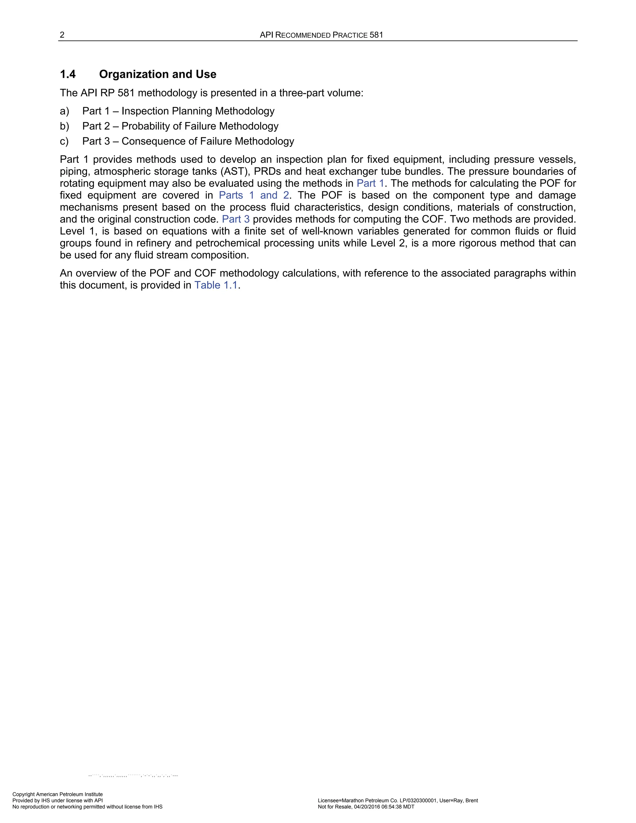
--````,`,,,,,,`,,,,,,```````,`-`-`,,`,,`,`,,`---](https://image.slidesharecdn.com/api581-3rdedition-april2016-240227010601-3bf73ab5/75/Norma-API-581-3rd-Edition-April-2016-pdf-1-2048.jpg)

![1
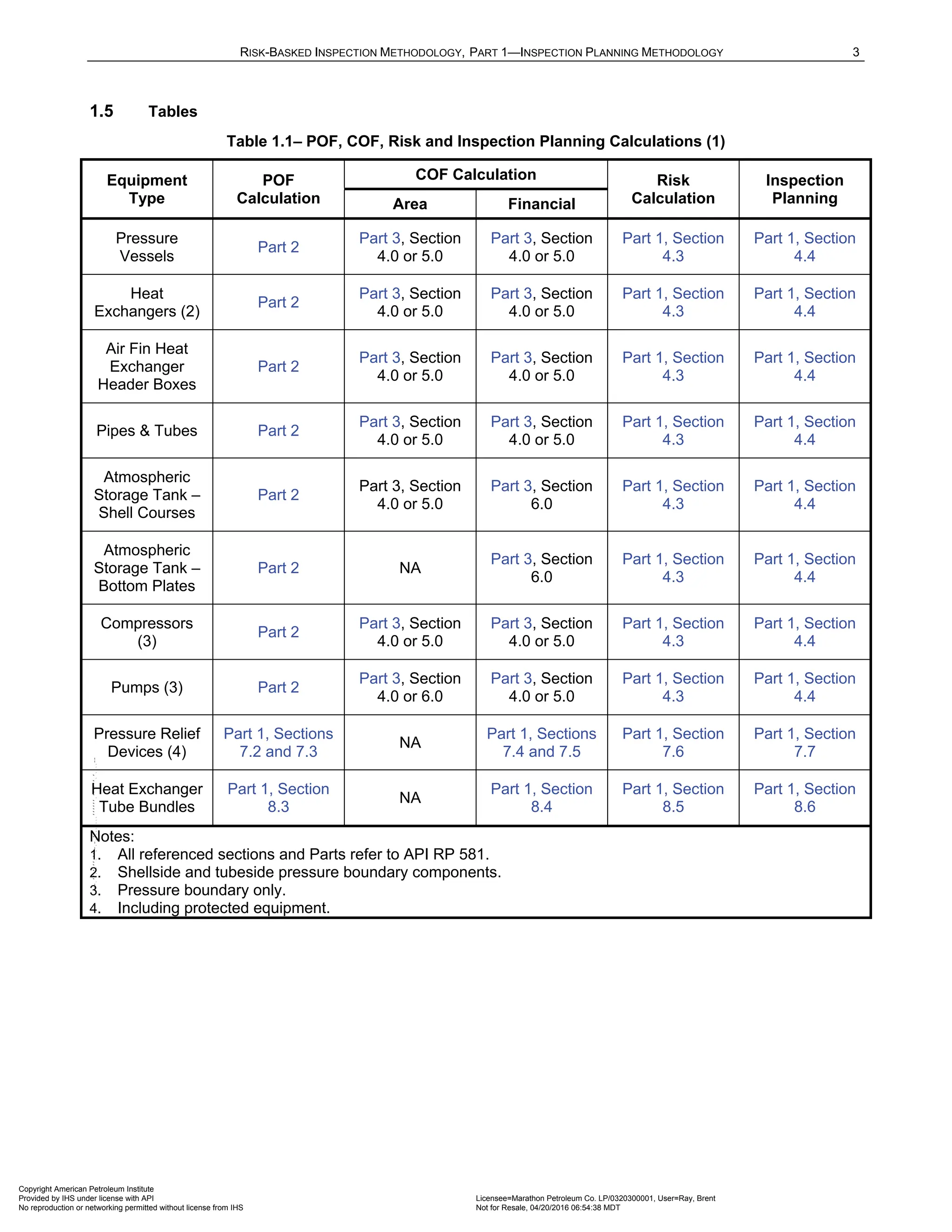
Risk-Based Inspection Methodology
Part 1—Inspection Planning Methodology
1 Scope
1.1 Purpose
This recommended practice, API RP 581, Risk-Based Inspection Methodology, provides quantitative procedures
to establish an inspection program using risk-based methods for pressurized fixed equipment including pressure
vessel, piping, tankage, pressure relief devices (PRDs), and heat exchanger tube bundles. API RP 580 Risk-
Based Inspection [1] provides guidance for developing Risk-Based Inspection (RBI) programs on fixed
equipment in refining, petrochemical, chemical process plants and oil and gas production facilities. The intent is
for API RP 580 to introduce the principles and present minimum general guidelines for RBI while this
recommended practice provides quantitative calculation methods to determine an inspection plan.
1.2 Introduction
The calculation of risk outlined in API RP 581 involves the determination of a probability of failure (POF)
combined with the consequence of failure (COF). Failure is defined as a loss of containment from the pressure
boundary resulting in leakage to the atmosphere or rupture of a pressurized component. Risk increases as
damage accumulates during in-service operation as the risk tolerance or risk target is approached and an
inspection is recommended of sufficient effectiveness to better quantify the damage state of the component. The
inspection action itself does not reduce the risk; however, it does reduce uncertainty and therefore allows more
accurate quantification of the damage present in the component.
1.3 Risk Management
In most situations, once risks have been identified, alternate opportunities are available to reduce them.
However, nearly all major commercial losses are the result of a failure to understand or manage risk. In the past,
the focus of a risk assessment has been on-site safety-related issues. Presently, there is an increased
awareness of the need to assess risk resulting from:
a) On-site risk to employees,
b) Off-site risk to the community,
c) Business interruption risks, and
d) Risk of damage to the environment.
Any combination of these types of risks may be factored into decisions concerning when, where, and how to
inspect equipment.
The overall risk of a plant may be managed by focusing inspection efforts on the process equipment with higher
risk. API RP 581 provides a basis for managing risk by making an informed decision on inspection frequency,
level of detail, and types of non-destructive examination (NDE). It is a consensus document containing
methodology that owner-users may apply to their RBI programs. In most plants, a large percent of the total unit
risk will be concentrated in a relatively small percent of the equipment items. These potential higher risk
components may require greater attention, perhaps through a revised inspection plan. The cost of the increased
inspection effort can sometimes be offset by reducing excessive inspection efforts in the areas identified as
having lower risk. Inspection will continue to be conducted as defined in existing working documents, but
priorities, scope, and frequencies can be guided by the methodology contained in API RP 581.
This approach can be made cost-effective by integration with industry initiatives and government regulations,
such as Management of Process Hazards, Process Safety Management (OSHA 29 CFR 1910.119), or the
Environmental Protection Agency Risk Management Programs for Chemical Accident Release Prevention.
Copyright American Petroleum Institute
Provided by IHS under license with API Licensee=Marathon Petroleum Co. LP/0320300001, User=Ray, Brent
Not for Resale, 04/20/2016 06:54:38 MDT
No reproduction or networking permitted without license from IHS
--````,`,,,,,,`,,,,,,```````,`-`-`,,`,,`,`,,`---](https://image.slidesharecdn.com/api581-3rdedition-april2016-240227010601-3bf73ab5/75/Norma-API-581-3rd-Edition-April-2016-pdf-9-2048.jpg)

![RISK-BASKED INSPECTION METHODOLOGY, PART 1—INSPECTION PLANNING METHODOLOGY 17
4.1.2.2 Management Systems Factor
The management systems factor, MS
F , is an adjustment factor that accounts for the influence of the facility’s
management system on the mechanical integrity of the plant equipment. This factor accounts for the probability
that accumulating damage that may result in a loss of containment will be discovered prior to the occurrence.
The factor is also indicative of the quality of a facility’s mechanical integrity and process safety management
programs. This factor is derived from the results of an evaluation of facility or operating unit management
systems that affect plant risk. The management systems evaluation is provided in Part 2, Annex 2.A of this
document.
4.1.2.3 Damage Factors
The DF is determined based on the applicable damage mechanisms relevant to the materials of construction
and the process service, the physical condition of the component, and the inspection techniques used to
quantify damage. The DF modifies the industry generic failure frequency and makes it specific to the component
under evaluation.
DFs do not provide a definitive Fitness-For-Service (FFS) assessment of the component. Fitness-For-Service
analyses for pressurized component are covered by API 579-1/ASME FFS-1 [2]. The basic function of the DF is
to statistically evaluate the amount of damage that may be present as a function of time in service and the
effectiveness of the inspection activity to quantify that damage.
Methods for determining DFs are provided in Part 2 for the following damage mechanisms:
a) Thinning (both general and local)
b) Component lining damage
c) External damage (thinning and cracking)
d) Stress Corrosion Cracking (SCC)
e) High Temperature Hydrogen Attack (HTHA)
f) Mechanical fatigue (piping only)
g) Brittle fracture, including low-temperature brittle fracture, low alloy embrittlement, 885o
F embrittlement, and
sigma phase embrittlement
When more than one damage mechanism is active, the damage factor for each mechanism is calculated and
then combined, to determine a total DF for the component, as defined in Part 2, Section 3.4.2.
4.1.3 Two Parameter Weibull Distribution Method
The POF is computed from Equation (1.2):
( ) 1 exp
f
t
P t
β
η
= − −
(1.2)
Where the Weibull Shape Parameter, β , is unit-less, the Weibull characteristic life parameter, η , in years, and
t is the independent variable time in years.
4.1.3.1 Weibull Shape Factor
The β parameter, shows how the failure rate develops over time. Failure-modes related with infant mortality,
random, or wear-out have significant different β values. The β parameter determines which member of the
Weibull family of distributions is most appropriate. Different members have different shapes. The Weibull
distribution fits a broad range of life data compared to other distributions.
4.1.3.2 Weibull Characteristic Life
The η parameter is defined as the time at which 63.2% of the units have failed. For 1
β = , the MTTF and η
are equal. This is true for all Weibull distributions regardless of the shape factor. Adjustments are made to the
characteristic life parameter to increase or decrease the POF as a result of environmental factors, asset types,
Copyright American Petroleum Institute
Provided by IHS under license with API Licensee=Marathon Petroleum Co. LP/0320300001, User=Ray, Brent
Not for Resale, 04/20/2016 06:54:38 MDT
No reproduction or networking permitted without license from IHS
--````,`,,,,,,`,,,,,,```````,`-`-`,,`,,`,`,,`---](https://image.slidesharecdn.com/api581-3rdedition-april2016-240227010601-3bf73ab5/75/Norma-API-581-3rd-Edition-April-2016-pdf-25-2048.jpg)
![18 API RECOMMENDED PRACTICE 581
or as a result of actual inspection data. These adjustments may be viewed as an adjustment to the mean time to
failure (MTTF).
4.2 Consequence of Failure
4.2.1 Overview
Loss of containment of hazardous fluids from pressurized processing equipment may result in damage to
surrounding equipment, serious injury to personnel, production losses, and undesirable environmental impacts.
The consequence of a loss of containment is determined using well-established consequence analysis
techniques [3], [4], [5], [6], [7], and is expressed as an affected impact area or in financial terms. Impact areas
from event outcomes such as pool fires, flash fires, fireballs, jet fires, and vapor cloud explosions are quantified
based on the effects of thermal radiation and overpressure on surrounding equipment and personnel.
Additionally, cloud dispersion analysis methods are used to quantify the magnitude of flammable releases and
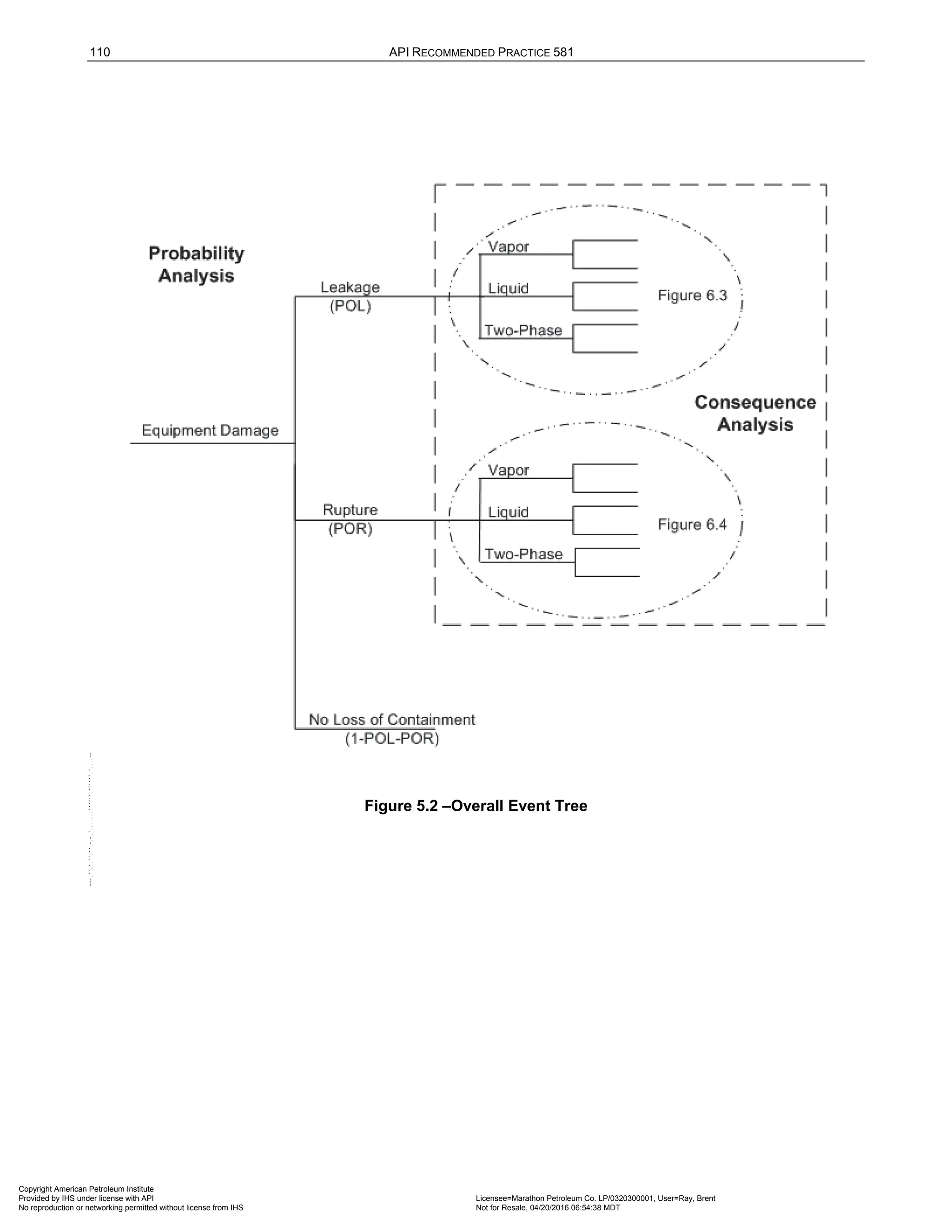
to determine the extent and duration of personnel exposure to toxic releases. Event trees are used to assess
the probability of each of the various event outcomes and to provide a mechanism for probability-weighting the
loss of containment consequences.
An overview of the COF methodology is provided in Part 3, Figure 4.1.
Methodologies for two levels of consequence analysis are provided in Part 3. A Level 1 consequence analysis
provides a method to estimate the consequence area based on lookup tables for a limited number of generic or
reference hazardous fluids. A Level 2 consequence analysis is more rigorous because it incorporates a detailed
calculation procedure that can be applied to a wider range of hazardous fluids.
4.2.2 Level 1 Consequence of Failure
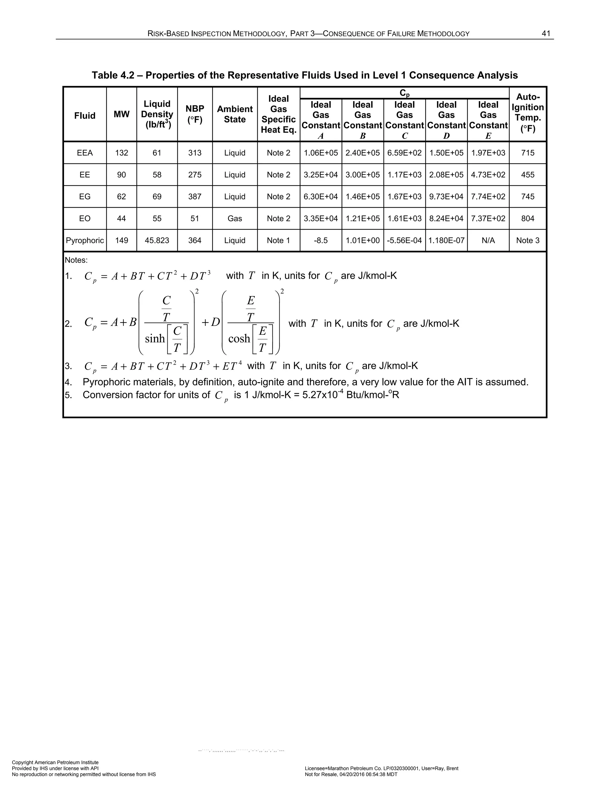
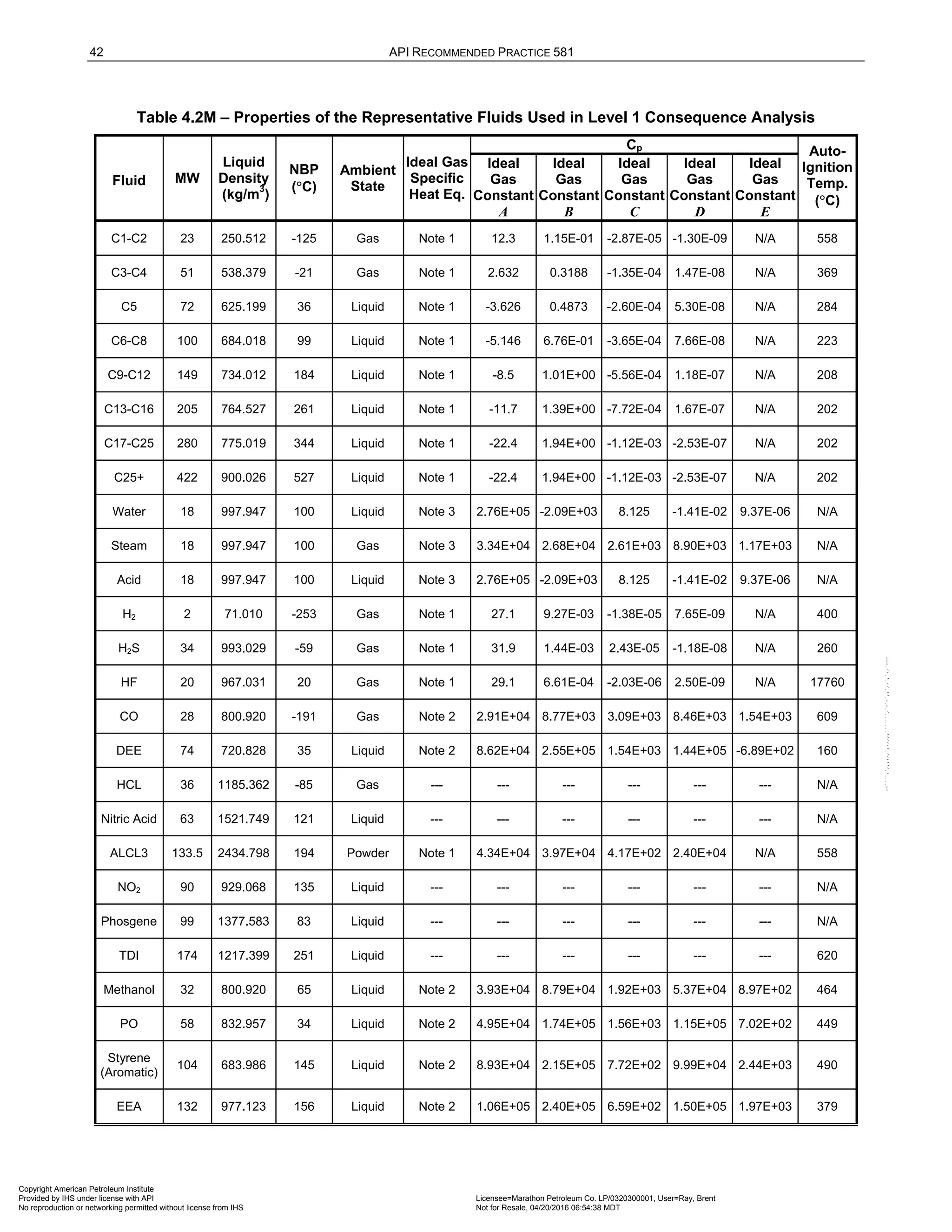
The Level 1 consequence analysis evaluates the consequence of hazardous releases for a limited number of
reference fluids (reference fluids are shown in Part 3, Table 4.1). The reference fluid that closely matches the
normal boiling point and molecular weight of the fluid contained within the process equipment should be used.
The flammable consequence area is then determined from a simple polynomial expression that is a function of
the release magnitude.
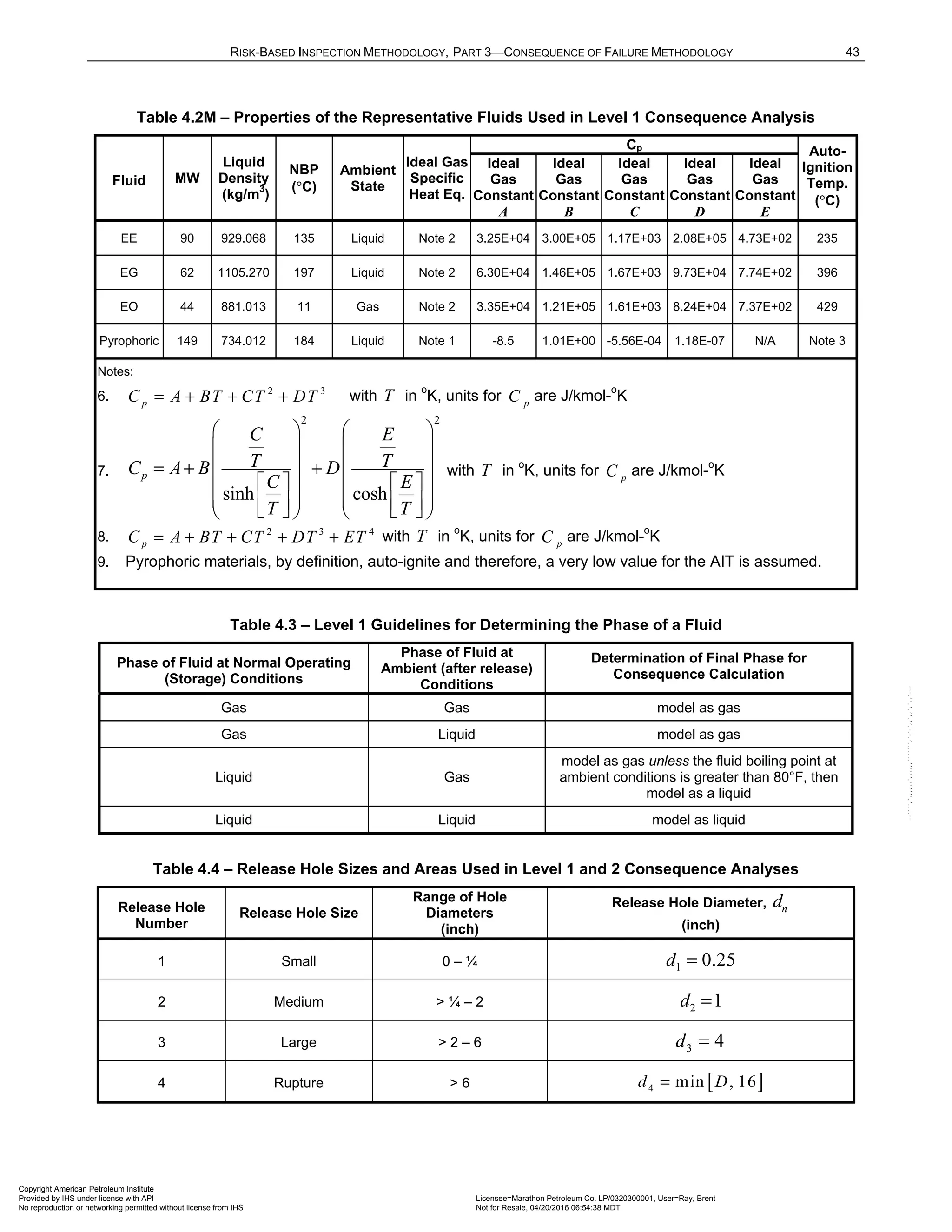
For each discrete hole size, release rates are calculated based on the phase of the fluid, as described in Part 3,
Section 4.3. These releases are then used in closed form equations to determine the flammable consequence.
For the Level 1 analysis, a series of consequence analyses were performed to generate consequence areas as
a function of the reference fluid and release magnitude. In these analyses, the major consequences were
associated with pool fires for liquid releases and vapor cloud explosions (VCEs) for vapor releases. Probabilities
of ignition, probabilities of delayed ignition, and other probabilities in the Level 1 event tree were selected based
on expert opinion for each of the reference fluids and release types (i.e., continuous or instantaneous). These
probabilities were constant and independent of release rate or mass. The closed form flammable consequence
area equation is shown in Equation (1.3) based on the analysis developed to calculate consequence areas.
b
CA a X
= ⋅ (1.3)
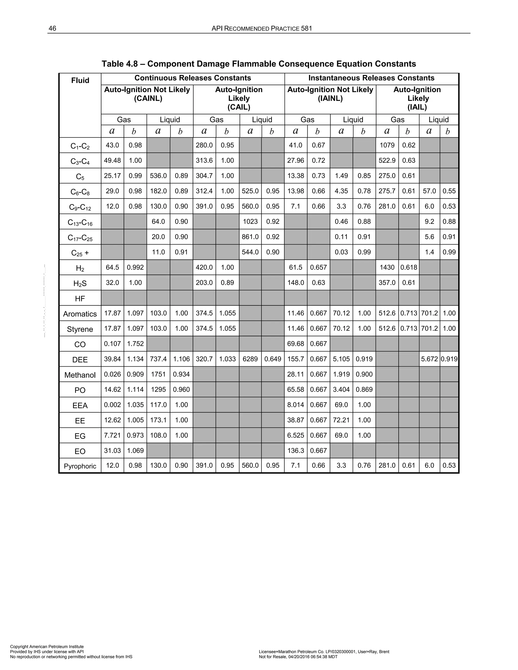
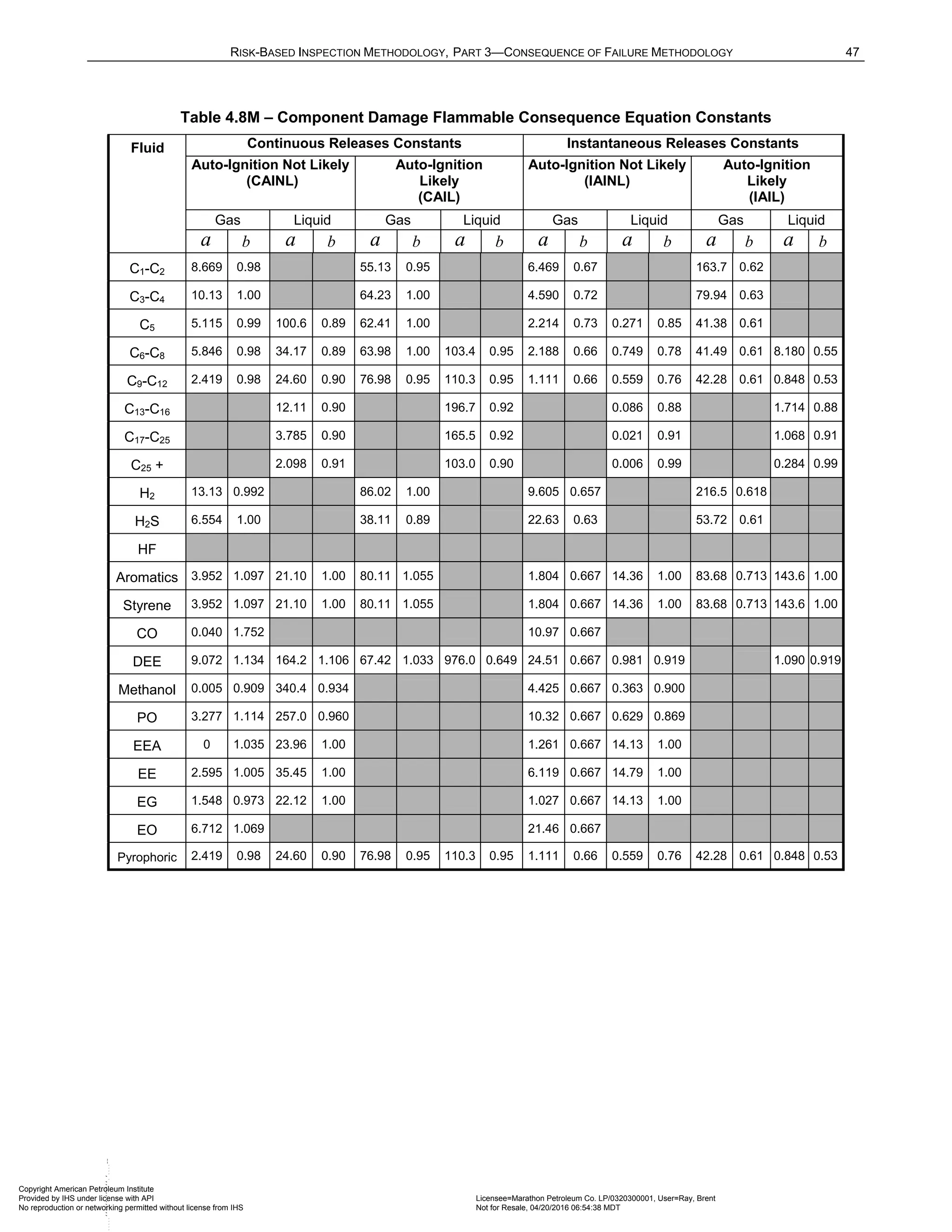
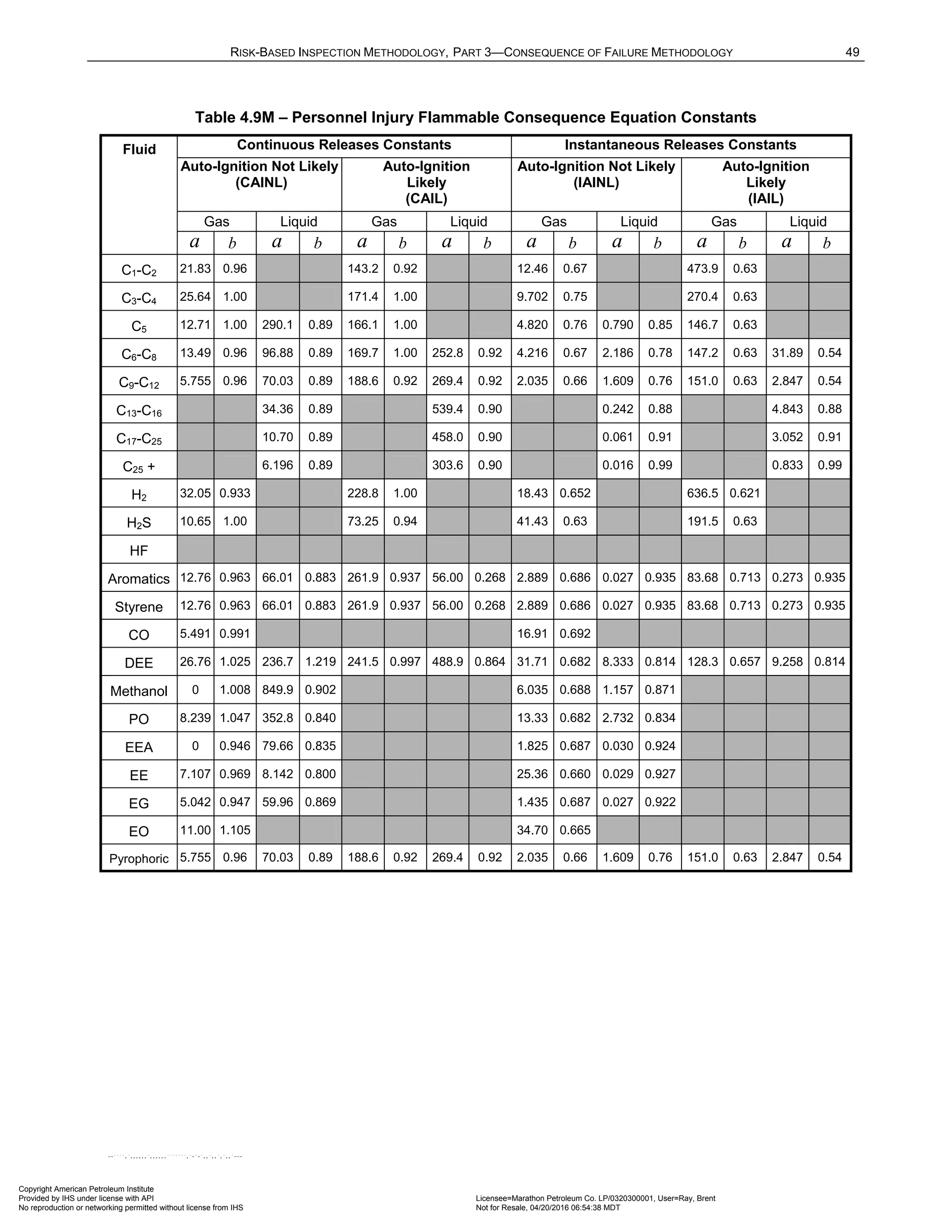
Values for variables a and b in Equation (1.3) are provided for the reference fluids in Part 3, Tables 4.8 and
4.9. If the fluid release is steady state and continuous (such as the case for small hole sizes), the release rate is
used for X in Equation (1.3). However, if the release is considered instantaneous (for example, as a result of a
vessel or pipe rupture), the release mass is used for X in Equation (1.3). The transition between a continuous
release and an instantaneous release is defined as a release where more than 4,536 kgs (10,000 lbs) of fluid
mass escapes in less than 3 minutes, see Part 3, Section 4.5.
The final flammable consequence areas are determined as a probability-weighted average of the individual
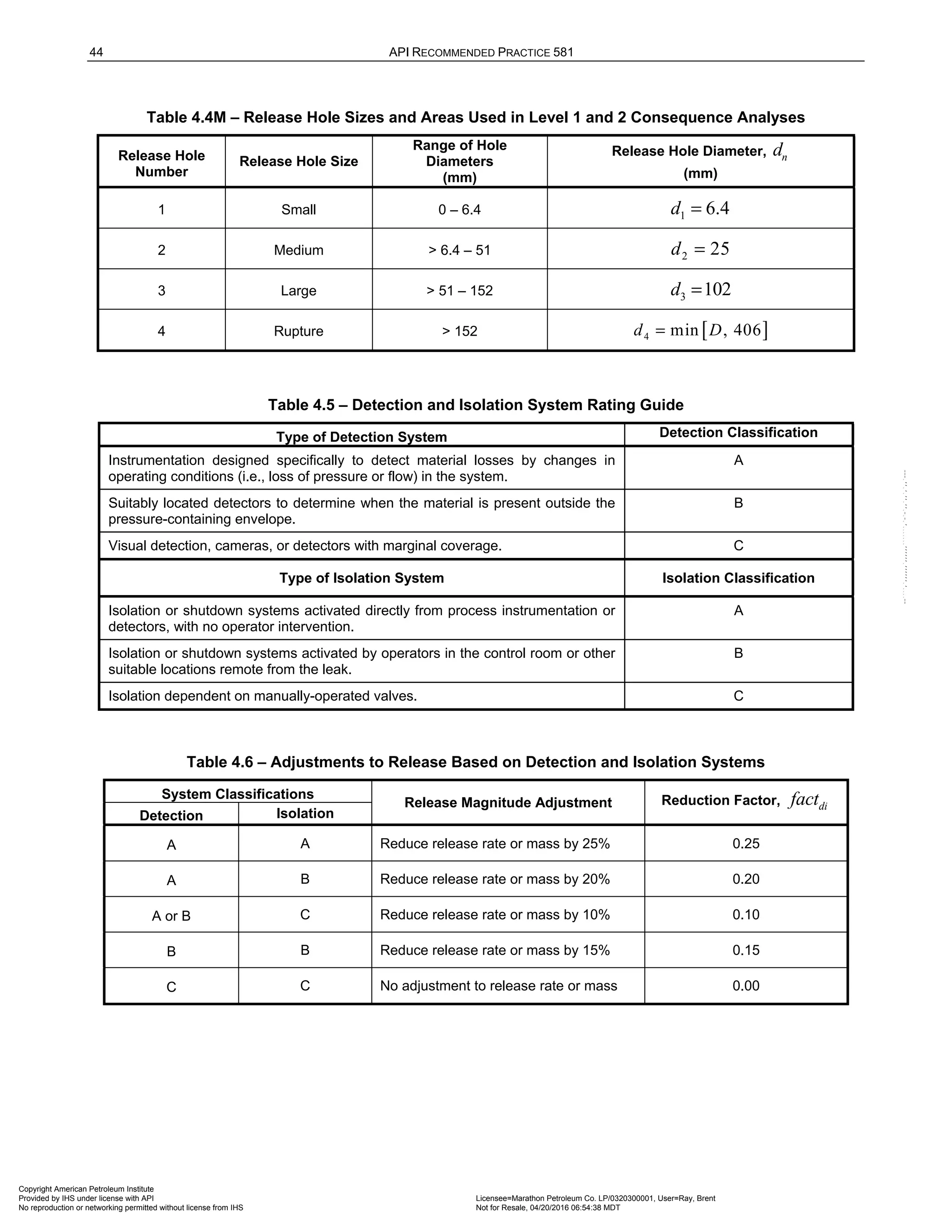
consequence areas calculated for each release hole size. Four hole sizes are used; the lowest hole size
represents a small leak and the largest hole size represents a rupture or complete release of contents. This is
performed for both the equipment damage and the personnel injury consequence areas. The probability
weighting uses the hole size distribution and the generic failure frequencies of the release hole sizes selected.
The equation for probability weighting of the flammable consequence areas is given by Equation (1.4).
Copyright American Petroleum Institute
Provided by IHS under license with API Licensee=Marathon Petroleum Co. LP/0320300001, User=Ray, Brent
Not for Resale, 04/20/2016 06:54:38 MDT
No reproduction or networking permitted without license from IHS
--````,`,,,,,,`,,,,,,```````,`-`-`,,`,,`,`,,`---](https://image.slidesharecdn.com/api581-3rdedition-april2016-240227010601-3bf73ab5/75/Norma-API-581-3rd-Edition-April-2016-pdf-26-2048.jpg)
![RISK-BASKED INSPECTION METHODOLOGY, PART 1—INSPECTION PLANNING METHODOLOGY 19
4
1
flam
n n
flam n
total
gff CA
CA
gff
=
⋅
=
(1.4)
The total generic failure frequency, total
gff , in the above equation is determined using Equation (1.5).
4
1
total n
n
gff gff
=
= (1.5)
The Level 1 consequence analysis is a method for approximating the consequence area of a hazardous
release. The inputs required are basic fluid properties (such as molecular weight [MW], density, and ideal gas
specific heat ratio, k ) and operating conditions. A calculation of the release rate or the available mass in the
inventory group (i.e., the inventory of attached equipment that contributes fluid mass to a leaking equipment
item) is also required. Once these terms are known, the flammable consequence area is determined from
Equations (1.3) and (1.4).
A similar procedure is used for determining the consequence associated with release of toxic chemicals such as
H2S, ammonia, or chlorine. Toxic impact areas are based on probit equations and can be assessed whether the
stream is pure or a percentage of a process stream.
4.2.3 Level 2 Consequence of Failure
A detailed procedure is provided for determining the consequence of loss of containment of hazardous fluids
from pressurized equipment. The Level 2 consequence analysis was developed as a tool to use where the
assumptions of Level 1 consequence analysis were not valid. Examples of where Level 2 calculations may be
desired or necessary are cited below:
a) The specific fluid is not represented adequately within the list of reference fluids provided in Part 3,
Table 4.1, including cases where the fluid is a wide-range boiling mixture or where the fluids toxic
consequence is not represented adequately by any of the reference fluids.
b) The stored fluid is close to its critical point, in which case, the ideal gas assumptions for the vapor release
equations are invalid.
c) The effects of two-phase releases, including liquid jet entrainment as well as rainout need to be included in
the methodology.
d) The effects of boiling liquid expanding vapor explosion (BLEVE) are to be included in the methodology.
e) The effects of pressurized non-flammable explosions, such as are possible when non-flammable
pressurized gases (e.g., air or nitrogen) are released during a vessel rupture, are to be included in the
methodology.
f) The meteorological assumptions used in the dispersion calculations that form the basis for the Level 1 COF
table lookups do not represent the site data.
The Level 2 consequence procedures presented in Part 3, Section 5.0 provide equations and background
information necessary to calculate consequence areas for several flammable and toxic event outcomes. A
summary of these events is provided in Part 3, Table 3.1.
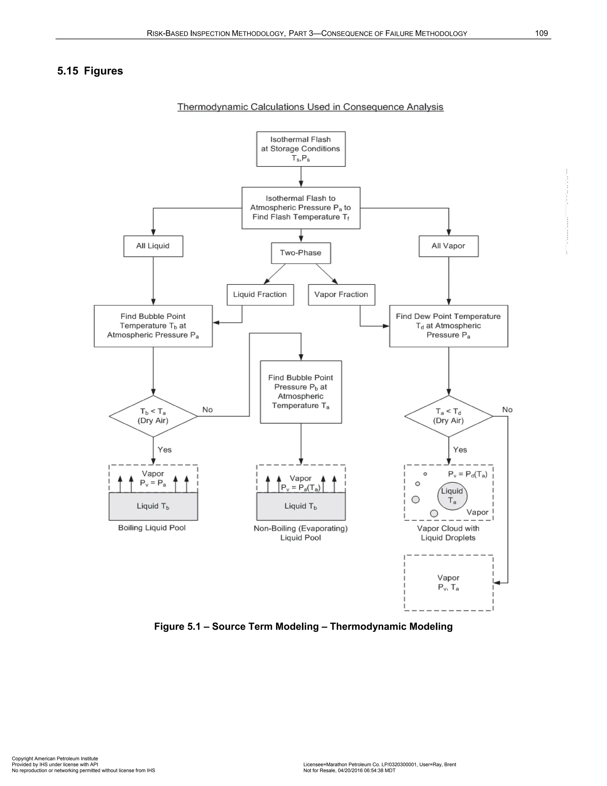
To perform Level 2 calculations, the actual composition of the fluid stored in the equipment is modeled. Fluid
property solvers are available that allow the analyst to calculate fluid physical properties more accurately. The
fluid solver also provides the ability to perform flash calculations to better determine the release phase of the
fluid and to account for two-phase releases. In many of the consequence calculations, physical properties of the
released fluid are required at storage conditions as well as conditions after release to the atmosphere.
Copyright American Petroleum Institute
Provided by IHS under license with API Licensee=Marathon Petroleum Co. LP/0320300001, User=Ray, Brent
Not for Resale, 04/20/2016 06:54:38 MDT
No reproduction or networking permitted without license from IHS
--````,`,,,,,,`,,,,,,```````,`-`-`,,`,,`,`,,](https://image.slidesharecdn.com/api581-3rdedition-april2016-240227010601-3bf73ab5/75/Norma-API-581-3rd-Edition-April-2016-pdf-27-2048.jpg)
![20 API RECOMMENDED PRACTICE 581
A cloud dispersion analysis must also be performed as part of a Level 2 consequence analysis to assess the
quantity of flammable material or toxic concentration throughout vapor clouds that are generated after a release
of volatile material. Modeling a release depends on the source term conditions, the atmospheric conditions, the
release surroundings, and the hazard being evaluated. Employment of many commercially available models,
including SLAB or DEGADIS [8], account for these important factors and will produce the desired data for the
Level 2 analysis.
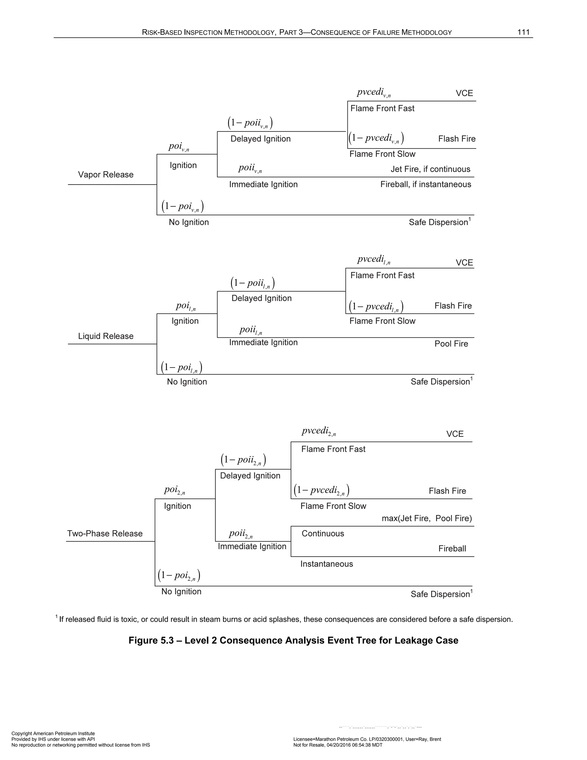
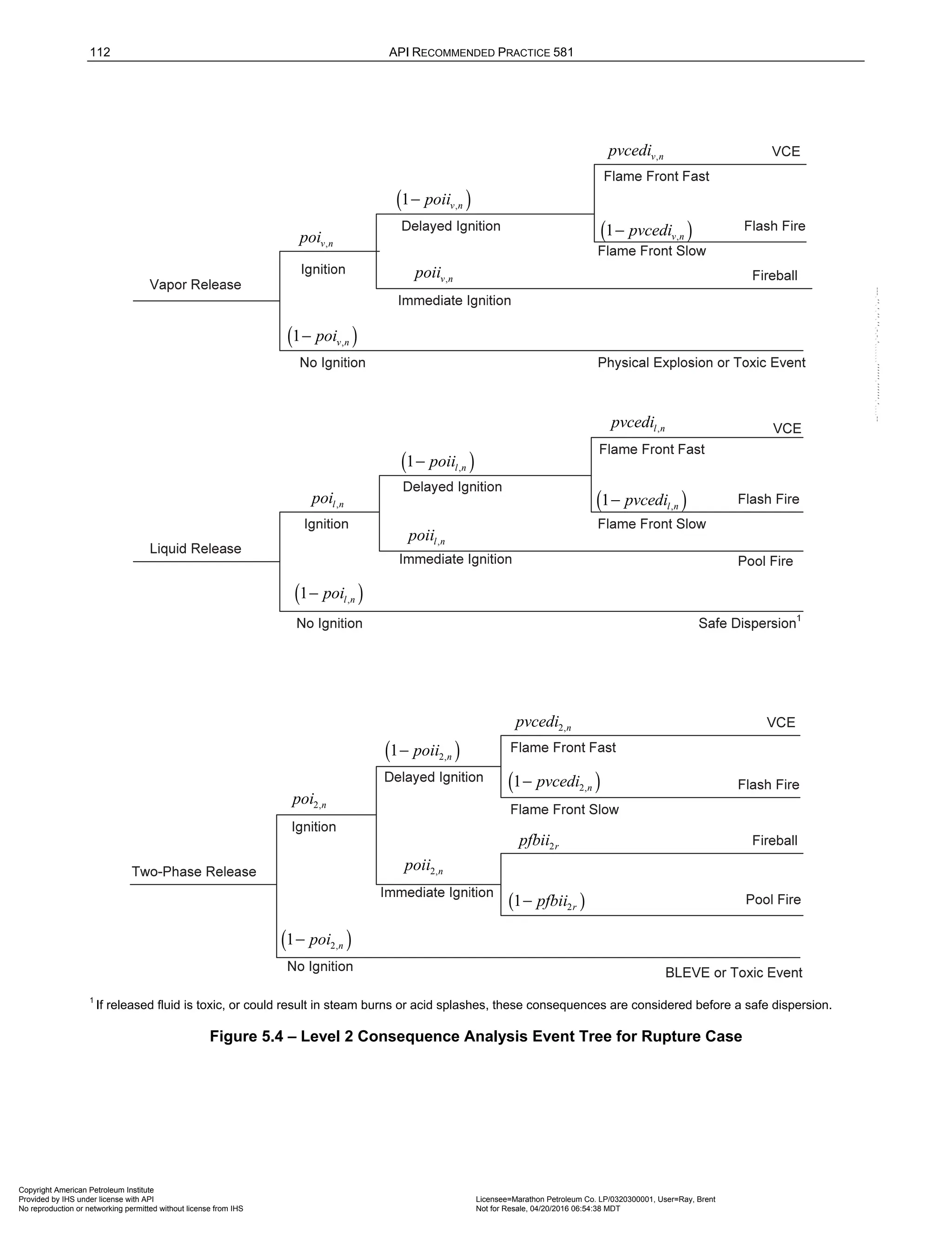
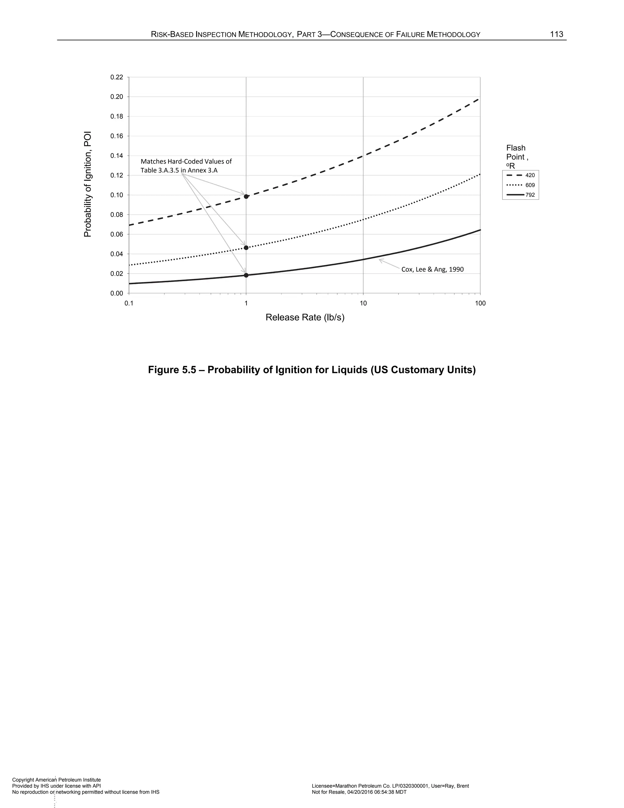
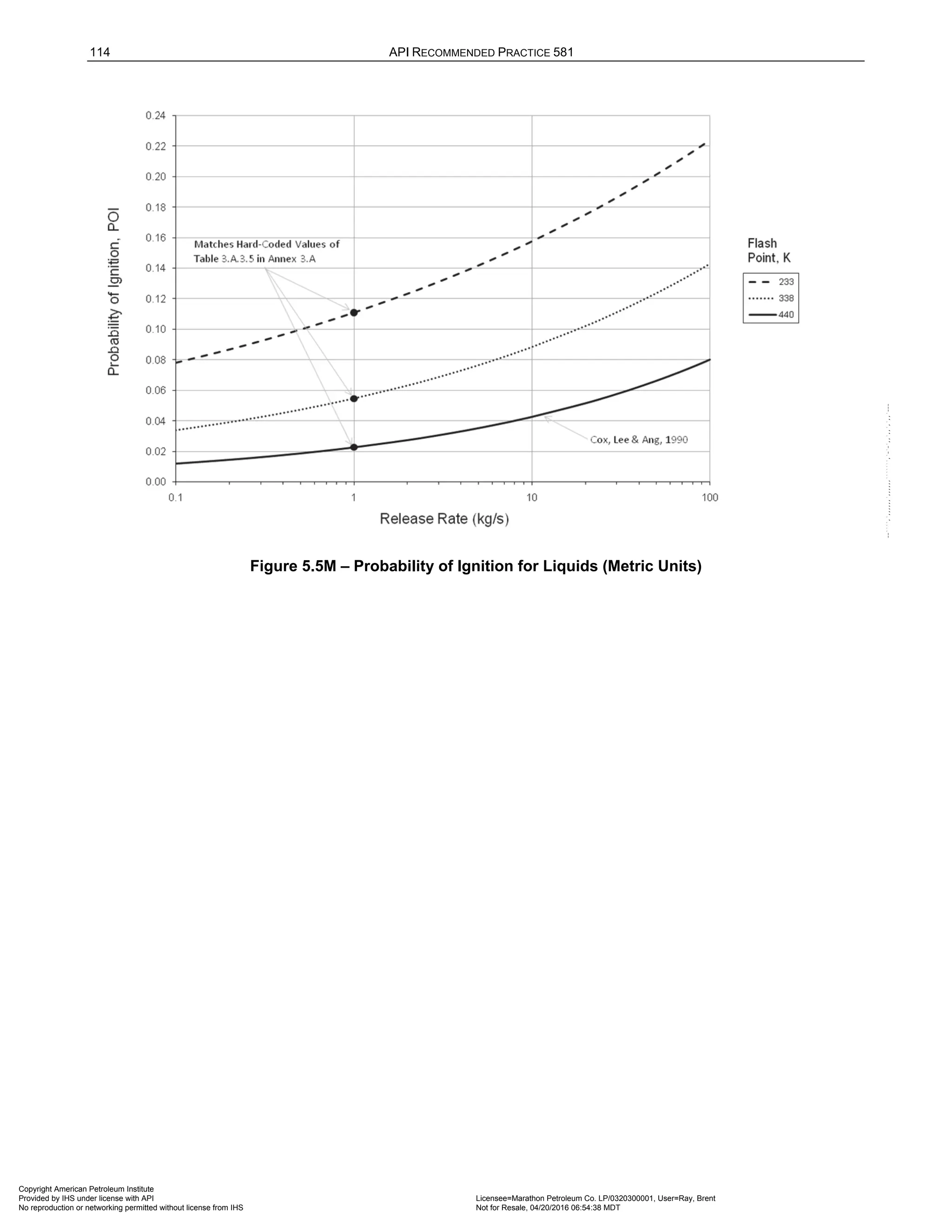
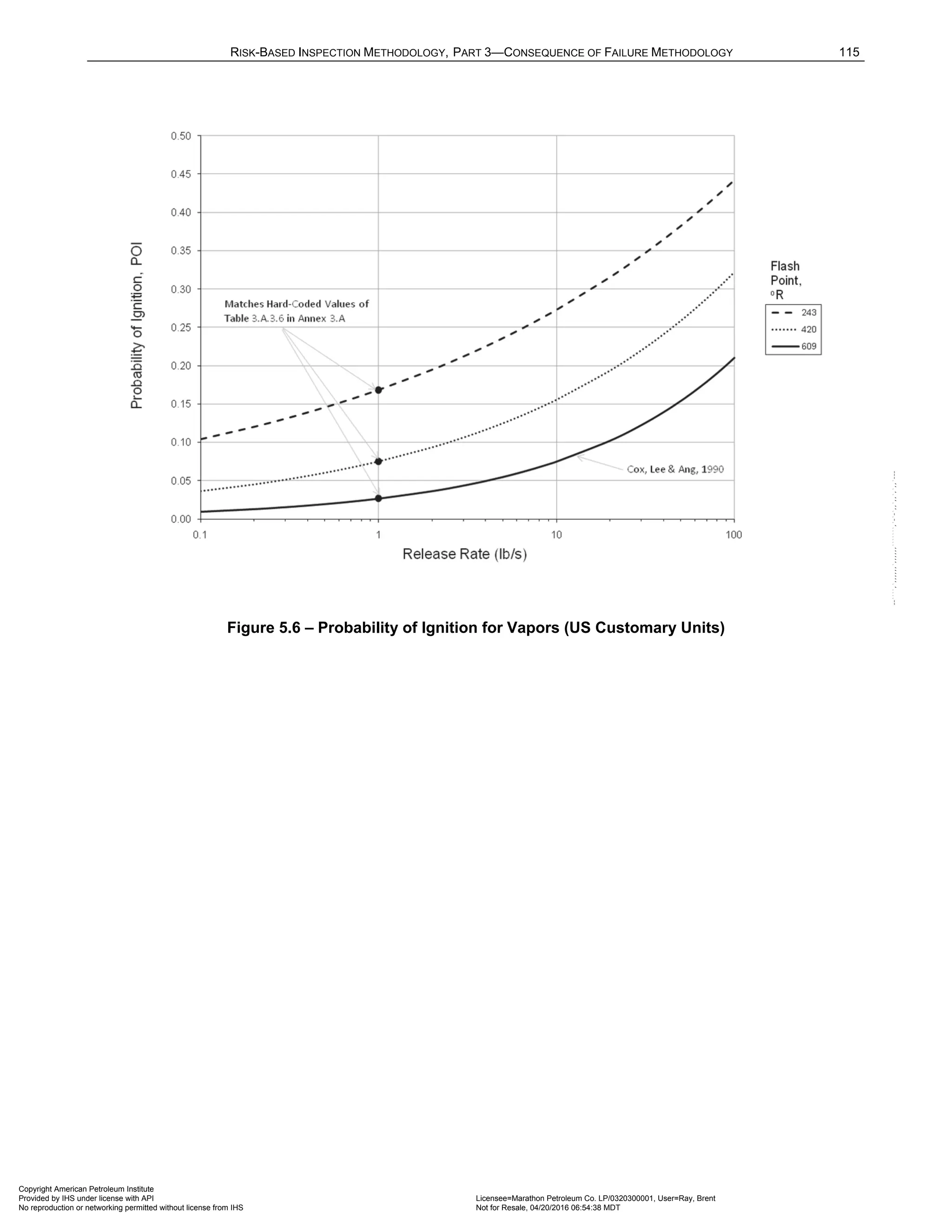
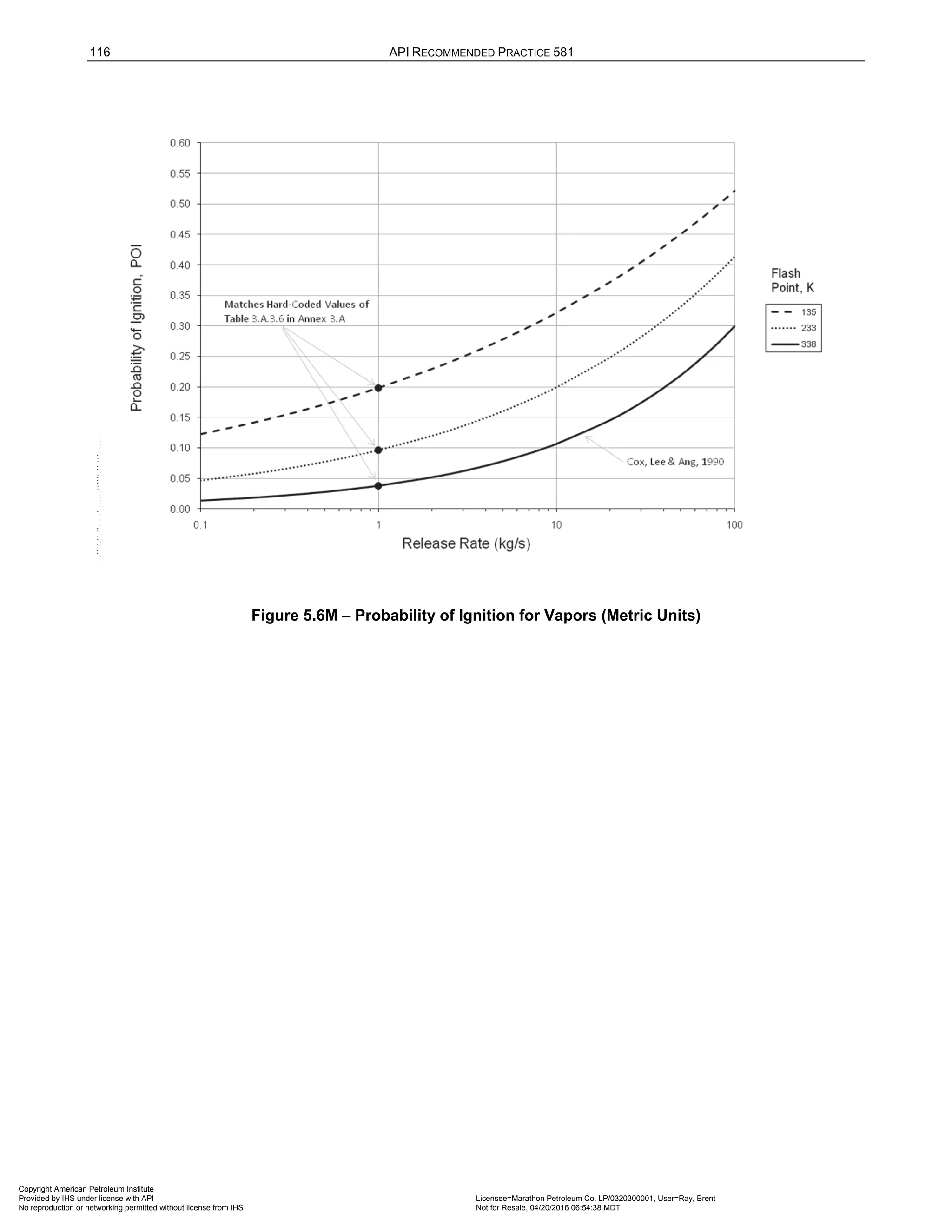
The event trees used in the Level 2 consequence analysis are shown in Part 3, Figures 5.3 and 5.4.
Improvement in the calculations of the probabilities on the event trees have been made in the Level 2
procedure. Unlike the Level 1 procedure, the probabilities of ignition on the event tree are not constant with
release magnitude. Consistent with the work of Cox, Lee, and Ang [9], the Level 2 event tree ignition
probabilities are directly proportional to the release rate. The probabilities of ignition are also a function of the
flash point temperature of the fluid. The probability that an ignition will be a delayed ignition is also a function of
the release magnitude and how close the operating temperature is to the auto-ignition temperature (AIT) of the
fluid. These improvements to the event tree will result in consequence impact areas that are more dependent on
the size of release and the flammability and reactivity properties of the fluid being released.
4.3 Risk Analysis
4.3.1 Determination of Risk
In general, the calculation of risk is determined in accordance with Equation (1.6), as a function of time. The
equation combines the POF and the COF described in Sections 4.1 and 4.2, respectively.
( ) ( )
f f
R t P t C
= ⋅ (1.6)
The POF, ( )
f
P t , is a function of time since the DF shown in Equation (1.1) increases as the damage in the
component accumulates with time.
Process operational changes over time can result in changes to the POF and COF. Process operational
changes, such as in temperature, pressure or corrosive composition of the process stream, can result in an
increased POF due to increased damage rates or initiation of additional damage mechanisms. These types of
changes are identified by the plant Management of Change procedure and/or Integrity Operating Windows
program.
The COF is assumed to be invariant as a function of time. However, significant process changes can result in
COF changes. Process change examples may include changes in the flammable, toxic and
nonflammable/nontoxic components of the process stream, changes in the process stream from the production
source, variations in production over the lifetime of an asset or unit, and repurposing or revamping of an asset or
unit that impacts the operation and/or service of gas/liquid processing plant equipment. In addition, modifications
to detection, isolation and mitigation systems will affect the COF. As defined in API RP 580, a reassessment is
required when the original risk basis for the POF and/or COF changes significantly.
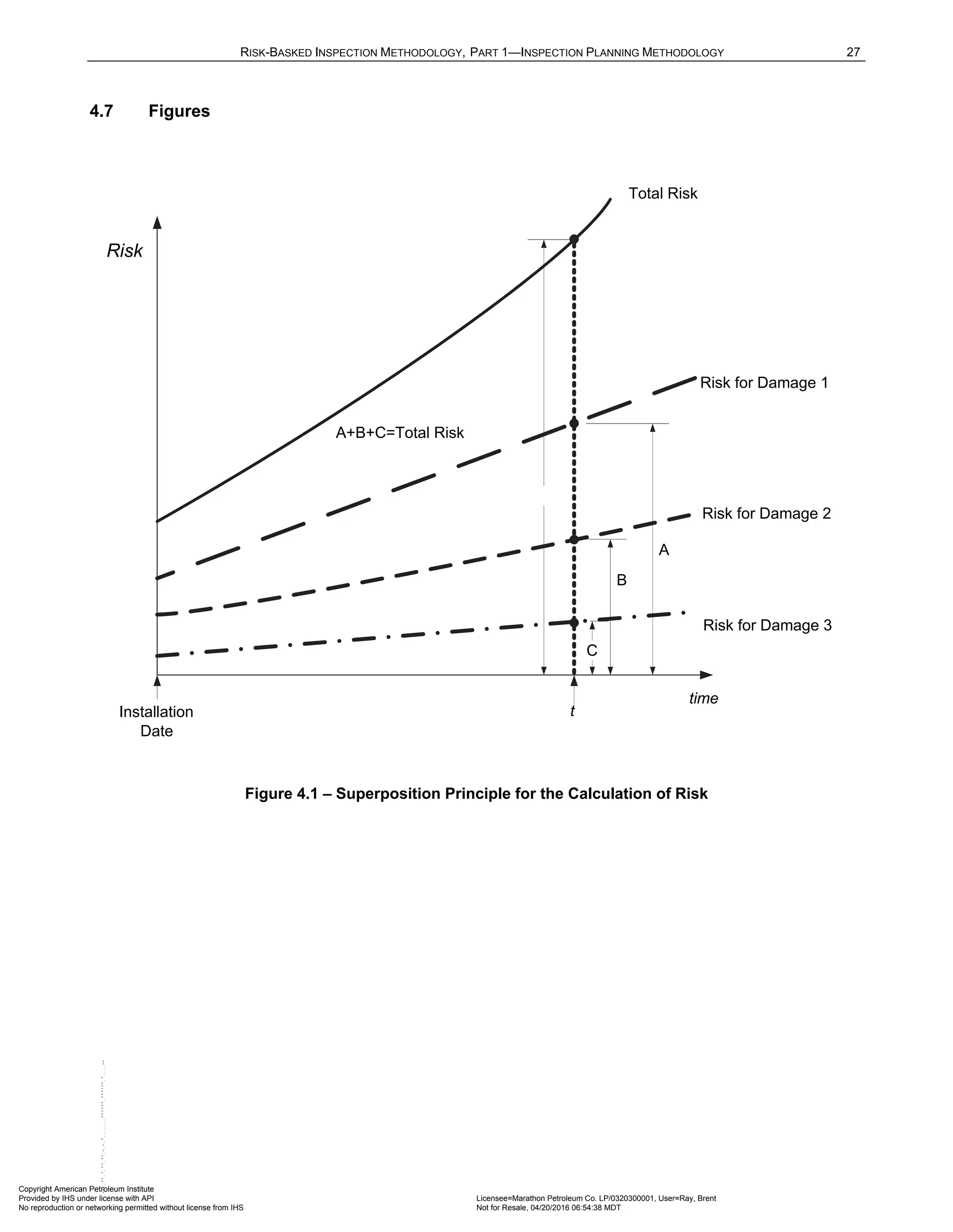
Equation (1.6) is rewritten in terms of Area and financial based risk, as shown in Equations (1.7) and (1.8).
( ) ( )
f
R t P t CA for Area Based Risk
= ⋅ − (1.7)
( ) ( )
f
R t P t FC for Financial Based Risk
= ⋅ − (1.8)
In these equations:
• CA is the consequence impact area expressed in units of area; and,
• FC is the financial consequence expressed in economic terms.
Note that in Equations (1.7) and (1.8), the risk varies with time due to the fact that the POF is a function of time.
Figure 4.1 illustrates that the risk associated with individual damage mechanisms can be added together by
superposition to provide the overall risk as a function of time.
Copyright American Petroleum Institute
Provided by IHS under license with API Licensee=Marathon Petroleum Co. LP/0320300001, User=Ray, Brent
Not for Resale, 04/20/2016 06:54:38 MDT
No reproduction or networking permitted without license from IHS
--````,`,,,,,,`,,,,,,```````,`-`-`,,`,,`,`,,`---](https://image.slidesharecdn.com/api581-3rdedition-april2016-240227010601-3bf73ab5/75/Norma-API-581-3rd-Edition-April-2016-pdf-28-2048.jpg)

![RISK-BASKED INSPECTION METHODOLOGY, PART 1—INSPECTION PLANNING METHODOLOGY 23
b) POF Target – A frequency of failure or leak (#/year) that is considered unacceptable and triggers the
inspection planning process.
c) DF Target – A damage state that reflects an unacceptable failure frequency factor greater than the generic
and triggers the inspection planning process.
d) COF Target – A level of unacceptable consequence in terms of consequence area (CA) or financial
consequence (FA) based on owner-user preference. Because risk driven by COF is not reduced by
inspection activities, risk mitigation activities to reduce release inventory or ignition are required.
e) Thickness Target – A specific thickness, often the minimum thickness, min
t , considered unacceptable,
triggering the inspection planning process.
f) Maximum Inspection Interval Target – A specific inspection frequency considered unacceptable, triggering
the inspection planning process. A maximum inspection interval may be set by the owner-user's corporate
standards or may be set based on a jurisdictional requirement
It is important to note that defining targets is the responsibility of the owner-user, and that specific target criteria
is not provided within this document. The above targets should be developed based on owner-user internal
guidelines and overall risk tolerance. Owner-users often have corporate risk criteria defining acceptable and
prudent levels of safety, environmental, and financial risks. These owner-user criteria should be used when
making RBI decisions since acceptable risk levels and risk management decision-making will vary among
companies.
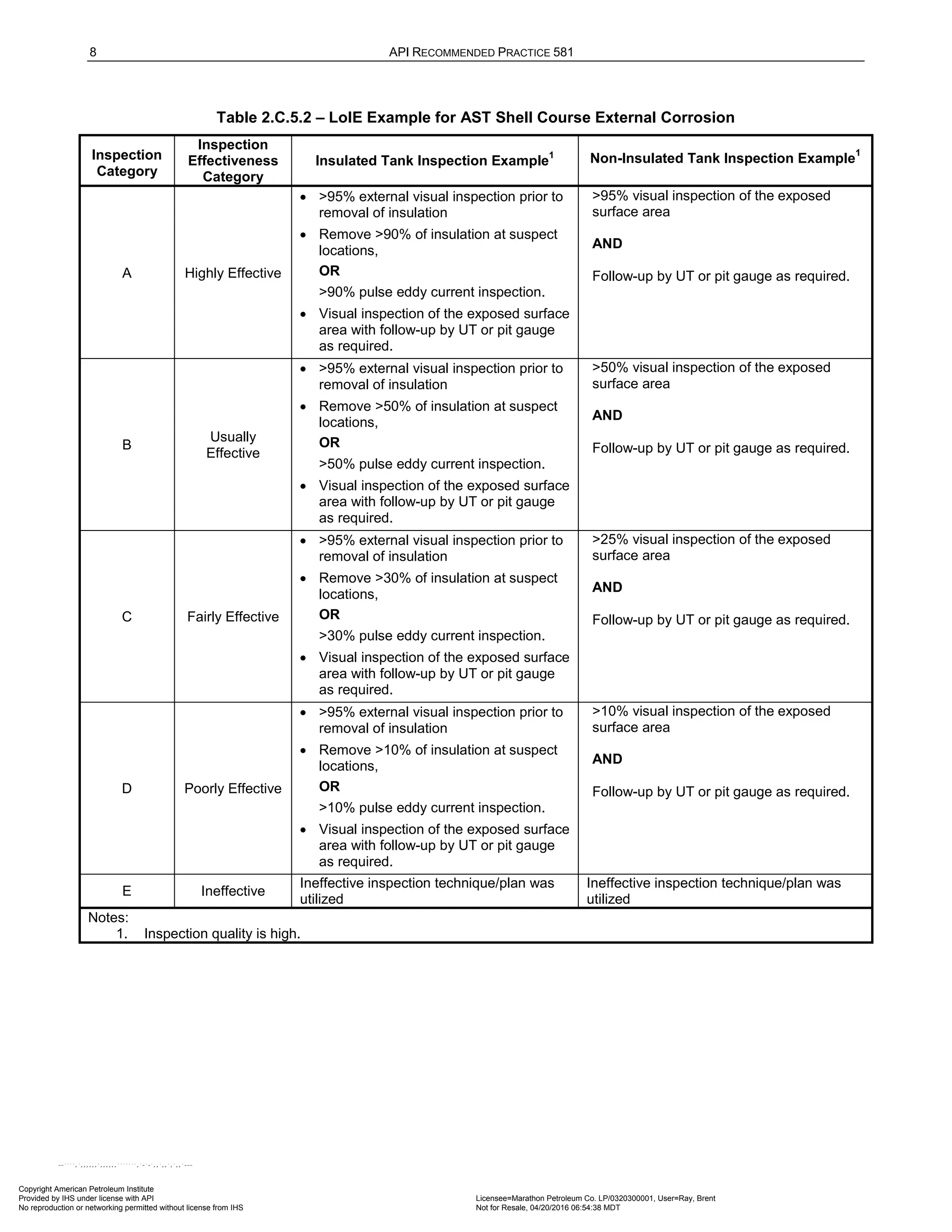
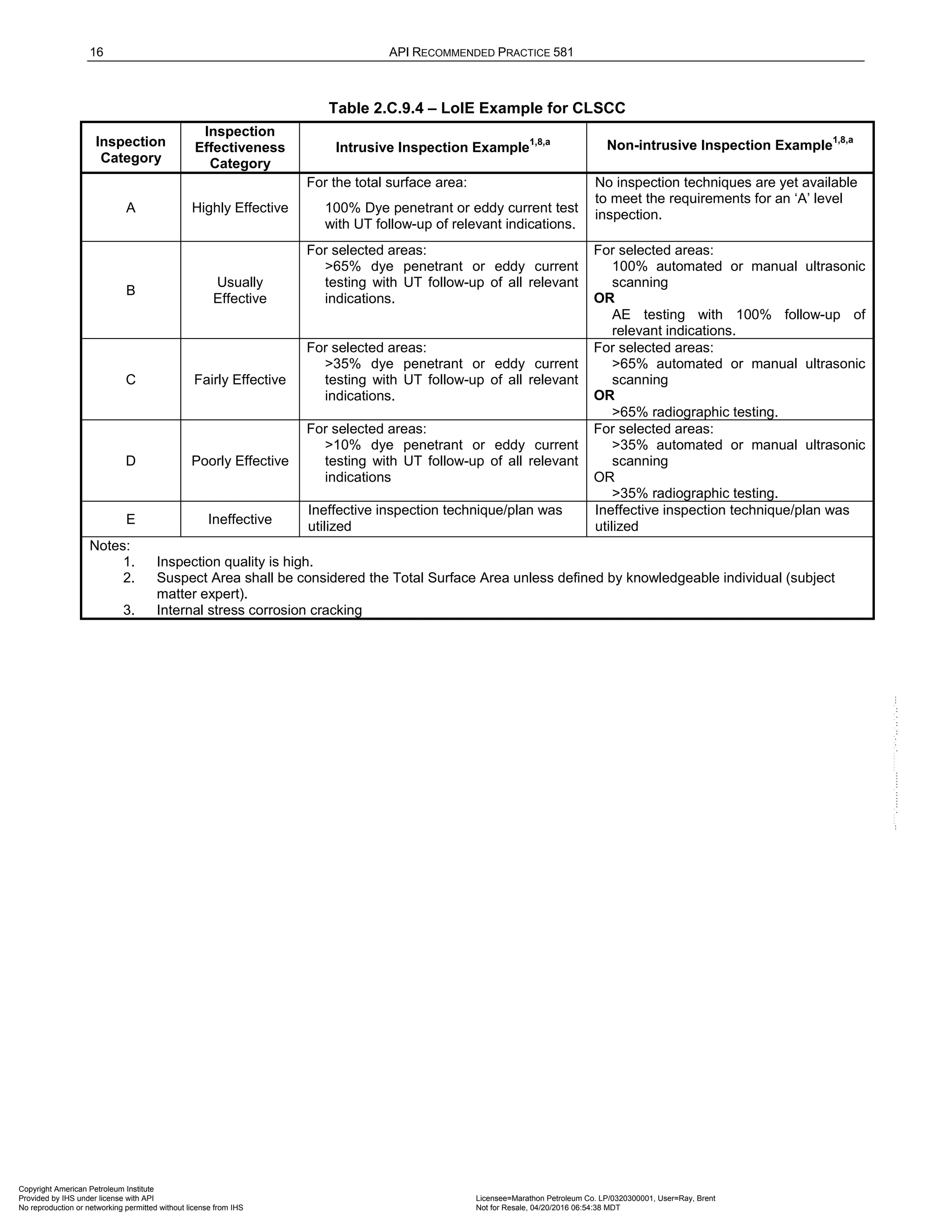
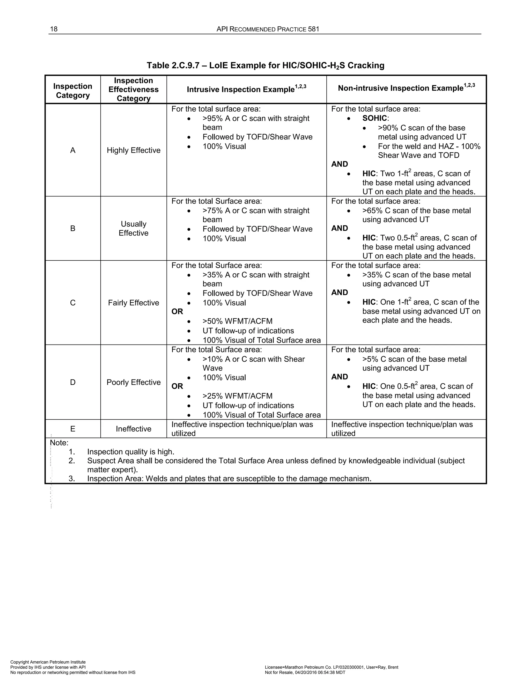
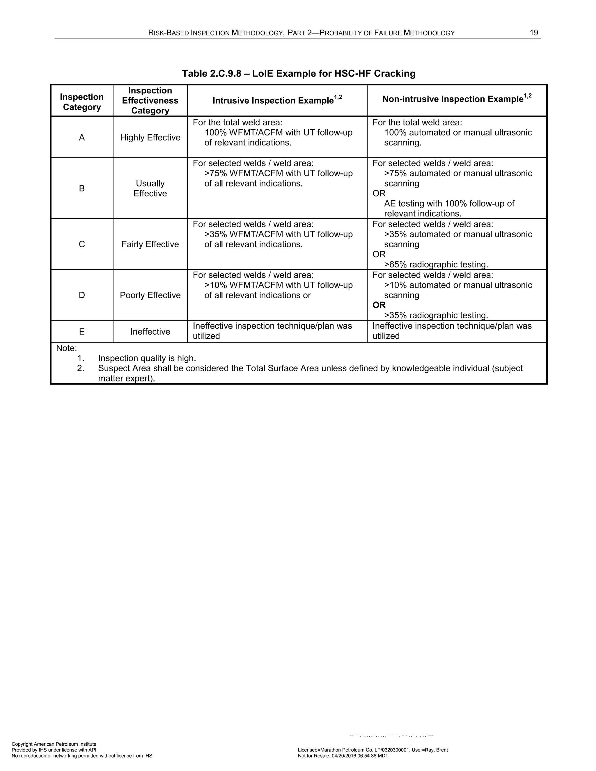
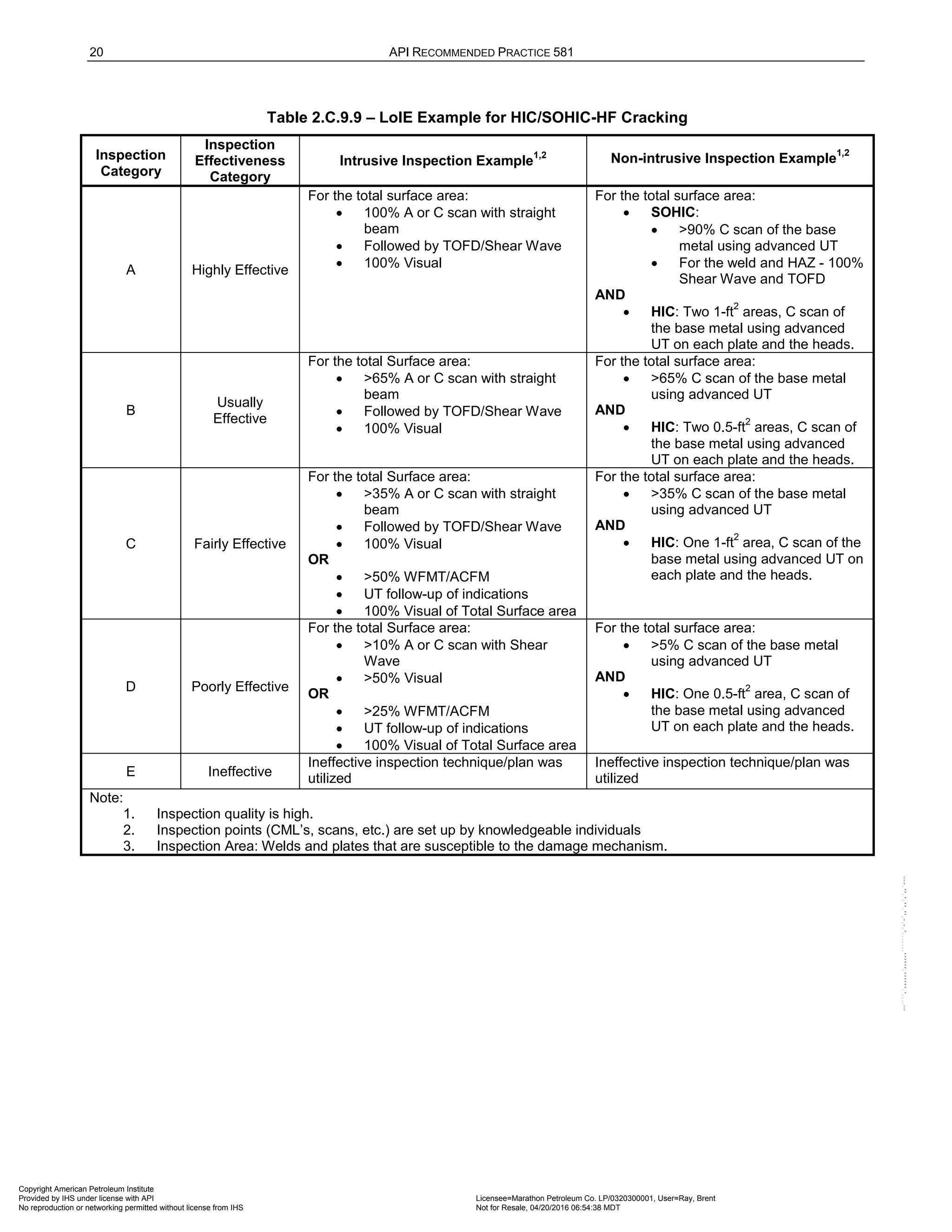
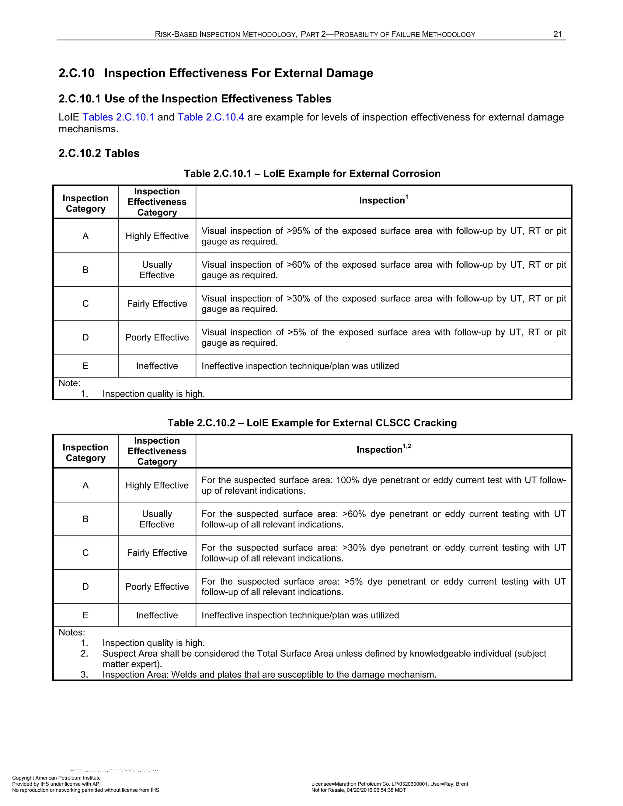
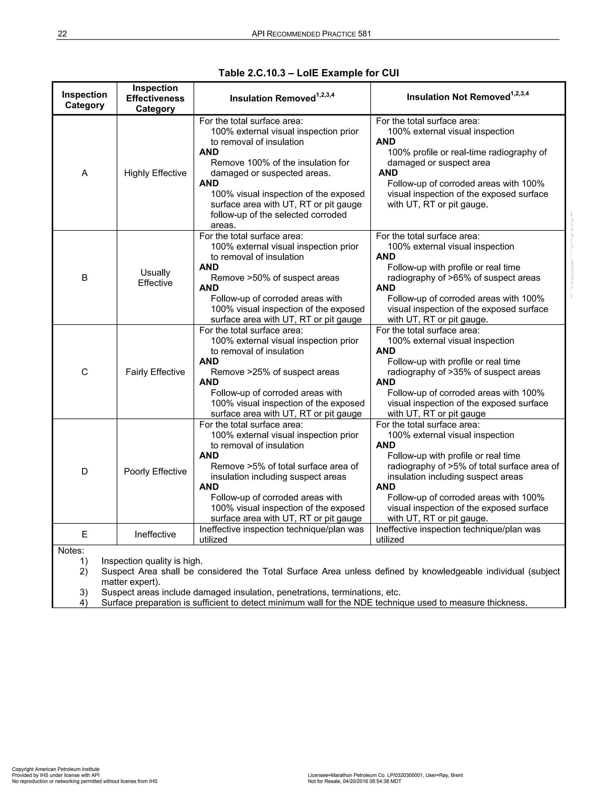
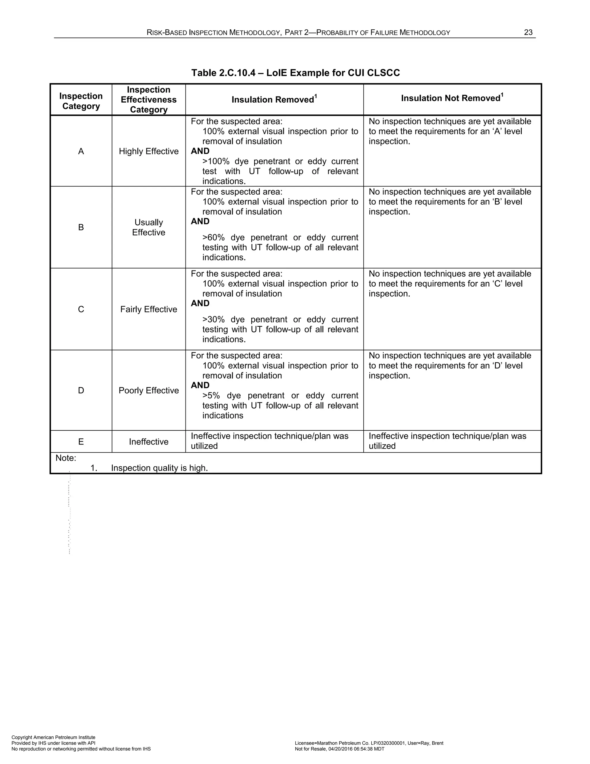
4.4.3 Inspection Effectiveness – The Value of Inspection
An estimate of the POF for a component depends on how well the independent variables of the limit state are
known [10] and understood. Using examples and guidance for inspection effectiveness provided in Part 2,
Annex 2.C, an inspection plan is developed, as risk results require. The inspection strategy is implemented to
obtain the necessary information to decrease uncertainty about the actual damage state of the equipment
by confirming the presence of damage, obtaining a more accurate estimate of the damage rate and
evaluating the extent of damage.
An inspection plan is the combination of NDE methods (i.e., visual, ultrasonic, radiographic, etc.), frequency of
inspection, and the location and coverage of an inspection to find a specific type of damage. Inspection plans
vary in their overall effectiveness for locating and sizing specific damage and understanding the extent of the
damage.
Inspection effectiveness is introduced into the POF calculation using Bayesian Analysis, which updates the POF
when additional data is gathered through inspection. The extent of reduction in the POF depends on the
effectiveness of the inspection to detect and quantify a specific damage type of damage mechanism. Therefore,
higher inspection effectiveness levels will reduce the uncertainty of the damage state of the component and
reduce the POF. The POF and associated risk may be calculated at a current and/or future time period using
Equations (1.9) or (1.10).
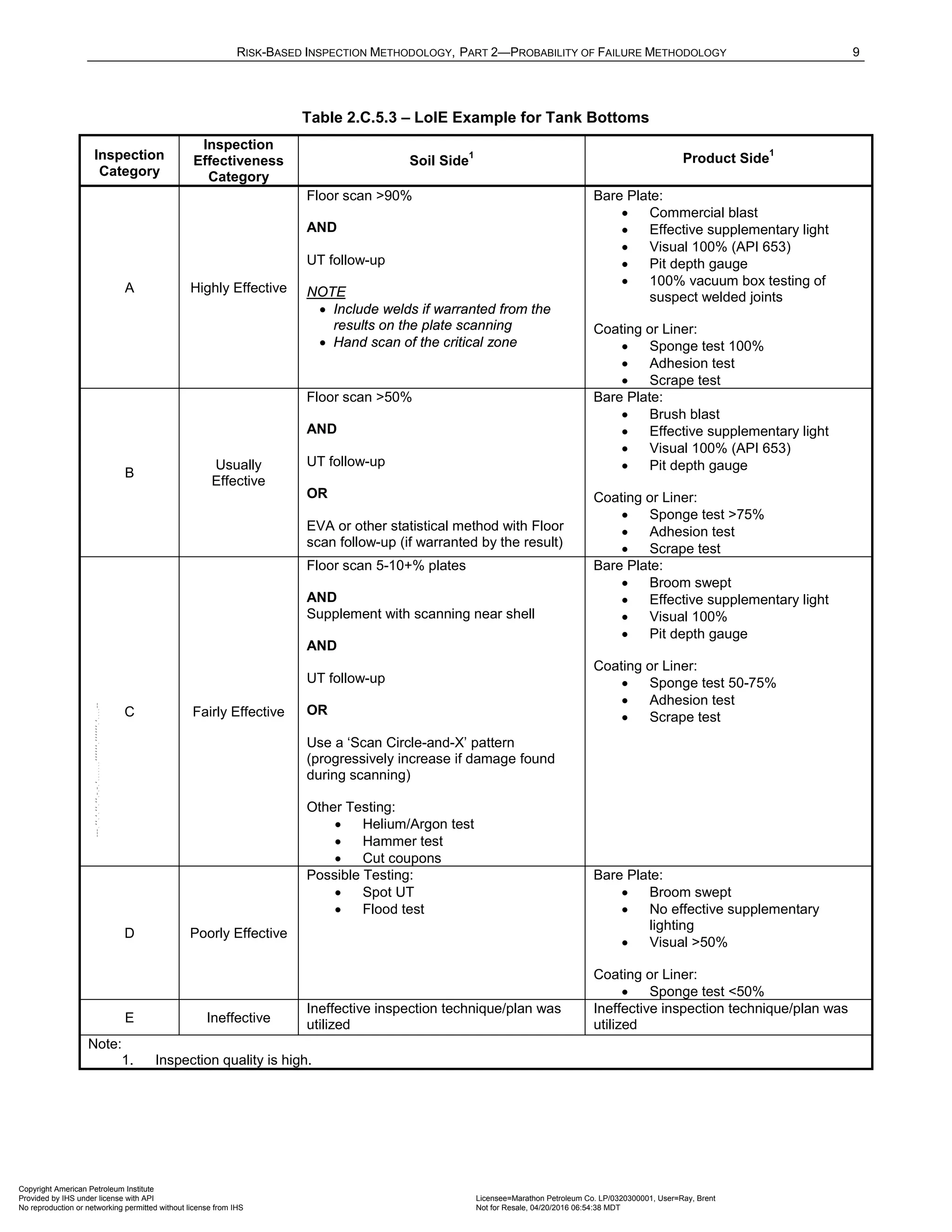
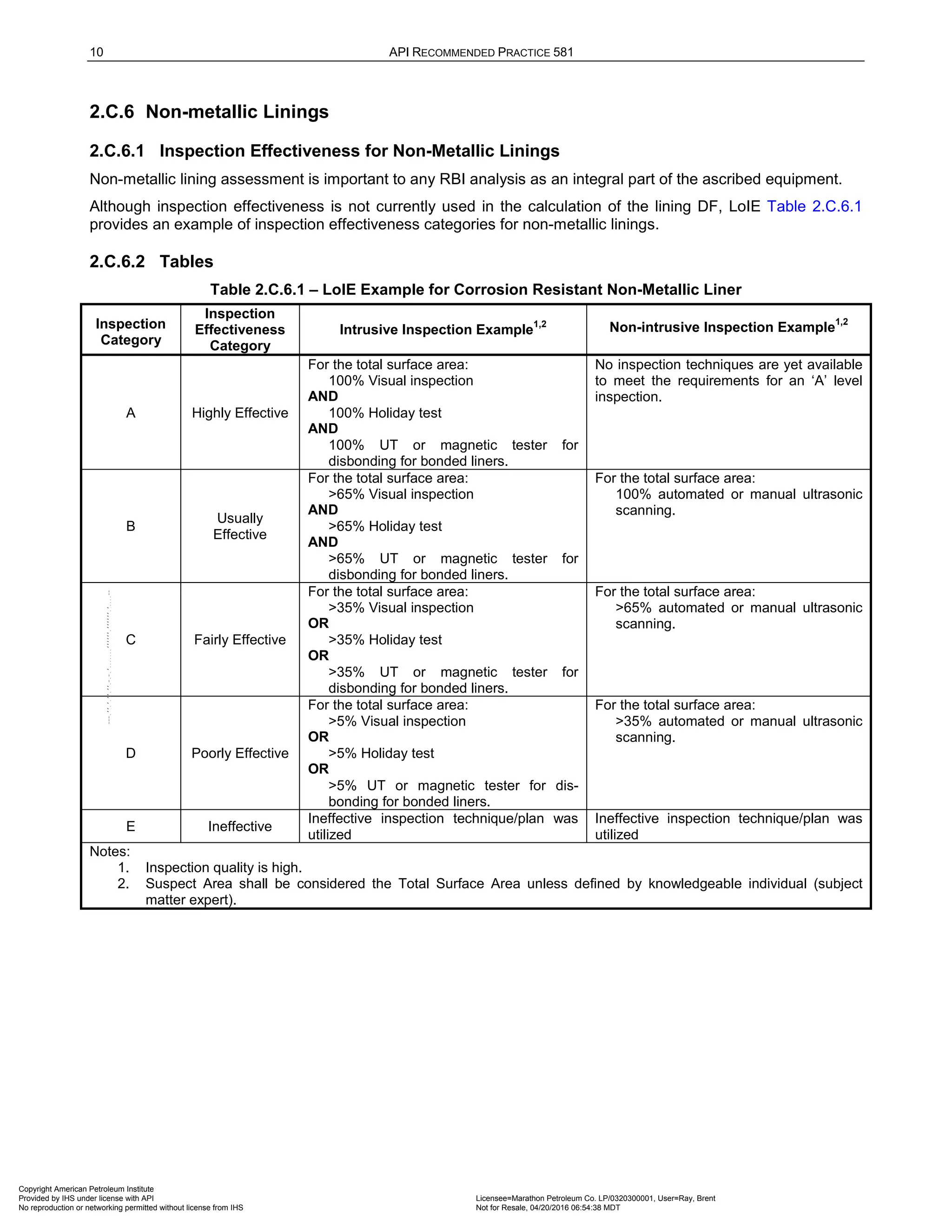
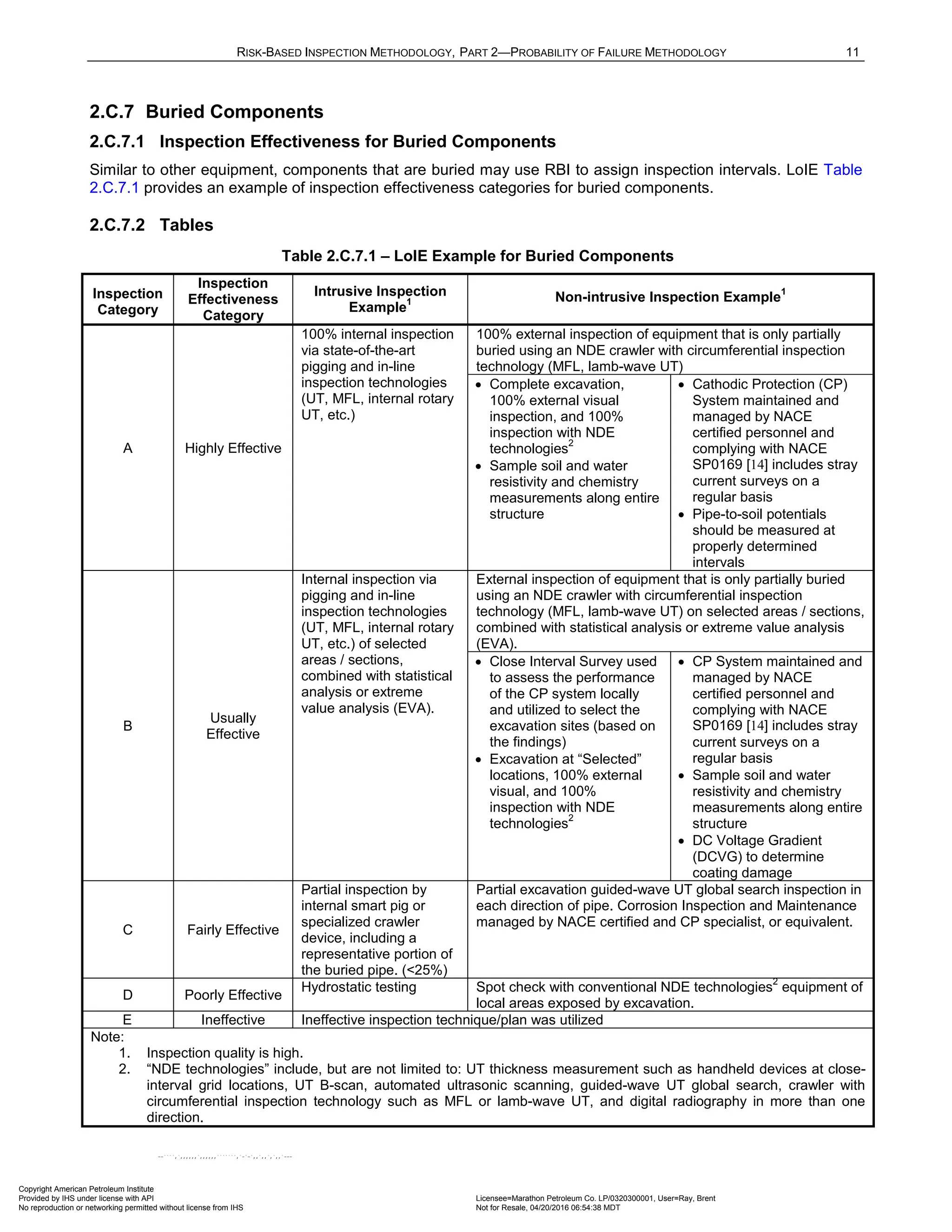
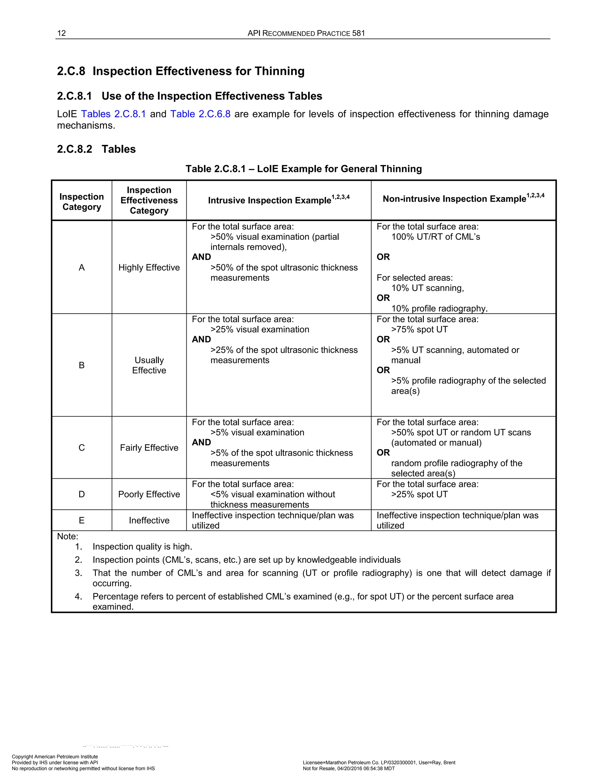
Examples of the levels of inspection effectiveness categories for various damage mechanisms and the
associated generic inspection plan (i.e., NDE techniques and coverage) for each damage mechanism are
provided in Part 2, Annex 2.C. These tables provide examples of the levels of generic inspection plans for a
specific damage mechanism. The tables are provided as a matter of example only, and it is the responsibility of
the owner-user to create, adopt, and document their own specific levels of inspection effectiveness tables.
4.4.4 Inspection Planning
An inspection Plan Date covers a defined Plan Period and includes one or more future maintenance
turnarounds. Within this Plan Period, three cases are possible based on predicted risk and the Risk Target.
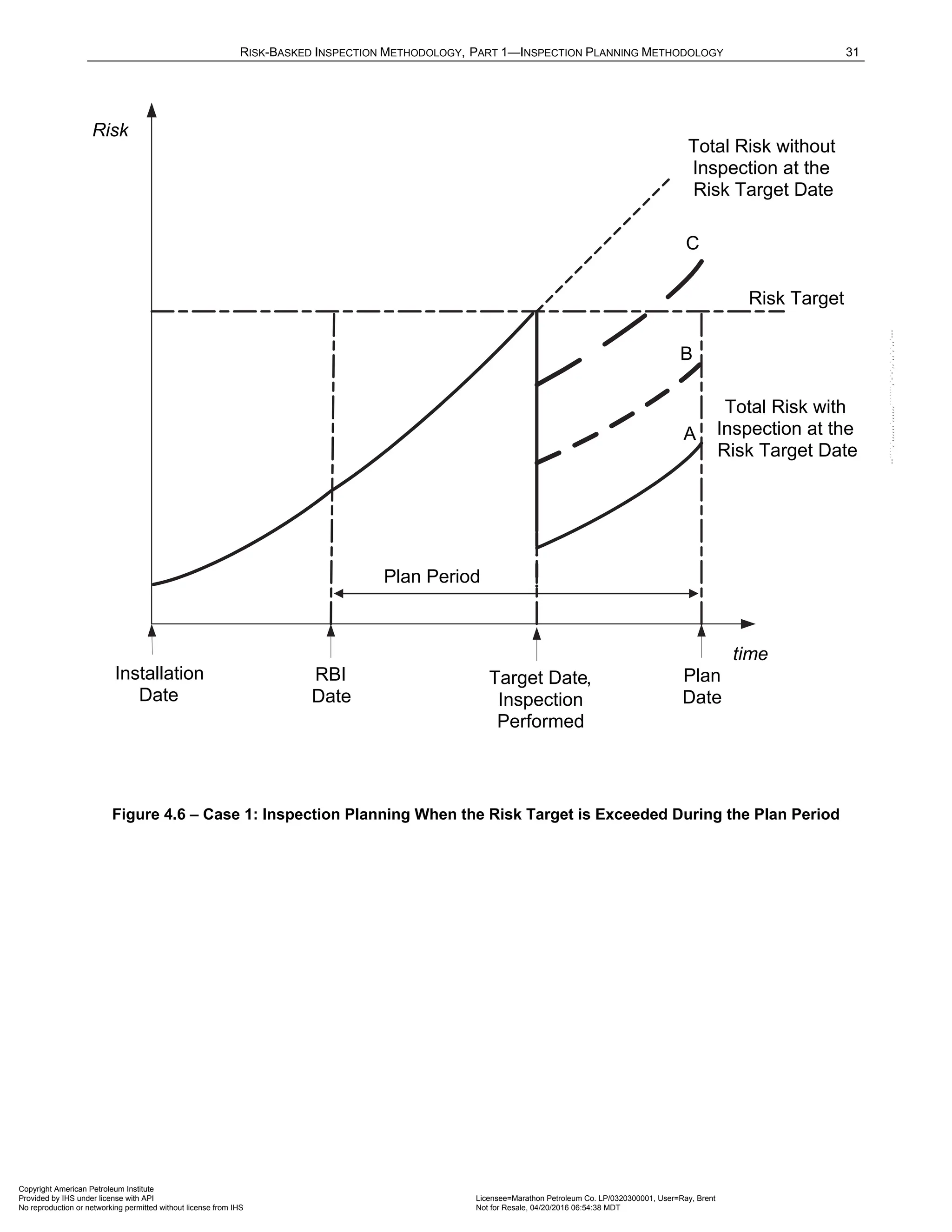
a) Case 1 – Risk Target is exceeded during the Plan Period – As shown in Figure 4.6, the inspection plan will
be based on the inspection effectiveness required to reduce the risk and maintain it below the risk target
through the plan period.
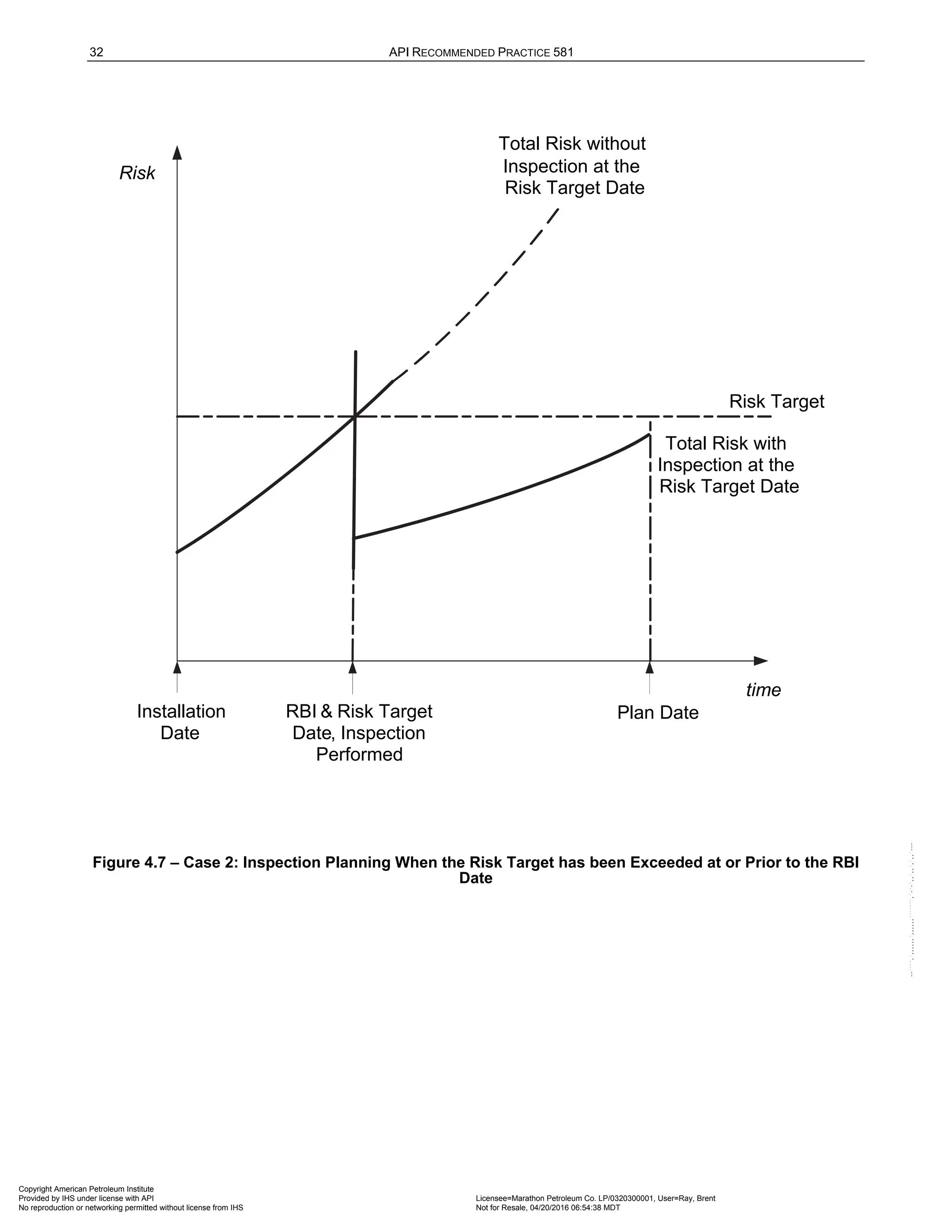
b) Case 2 – Risk exceeds the Risk Target at the time the RBI Date – As shown in Figure 4.7, the risk at the
start time of the RBI analysis, or RBI date, exceeds the risk target. An inspection is recommended to
reduce the risk below the risk target by the plan date.
Copyright American Petroleum Institute
Provided by IHS under license with API Licensee=Marathon Petroleum Co. LP/0320300001, User=Ray, Brent
Not for Resale, 04/20/2016 06:54:38 MDT
No reproduction or networking permitted without license from IHS
--````,`,,,,,,`,,,,,,```````,`-`-`,,`,,`,`,,`---](https://image.slidesharecdn.com/api581-3rdedition-april2016-240227010601-3bf73ab5/75/Norma-API-581-3rd-Edition-April-2016-pdf-31-2048.jpg)
![24 API RECOMMENDED PRACTICE 581
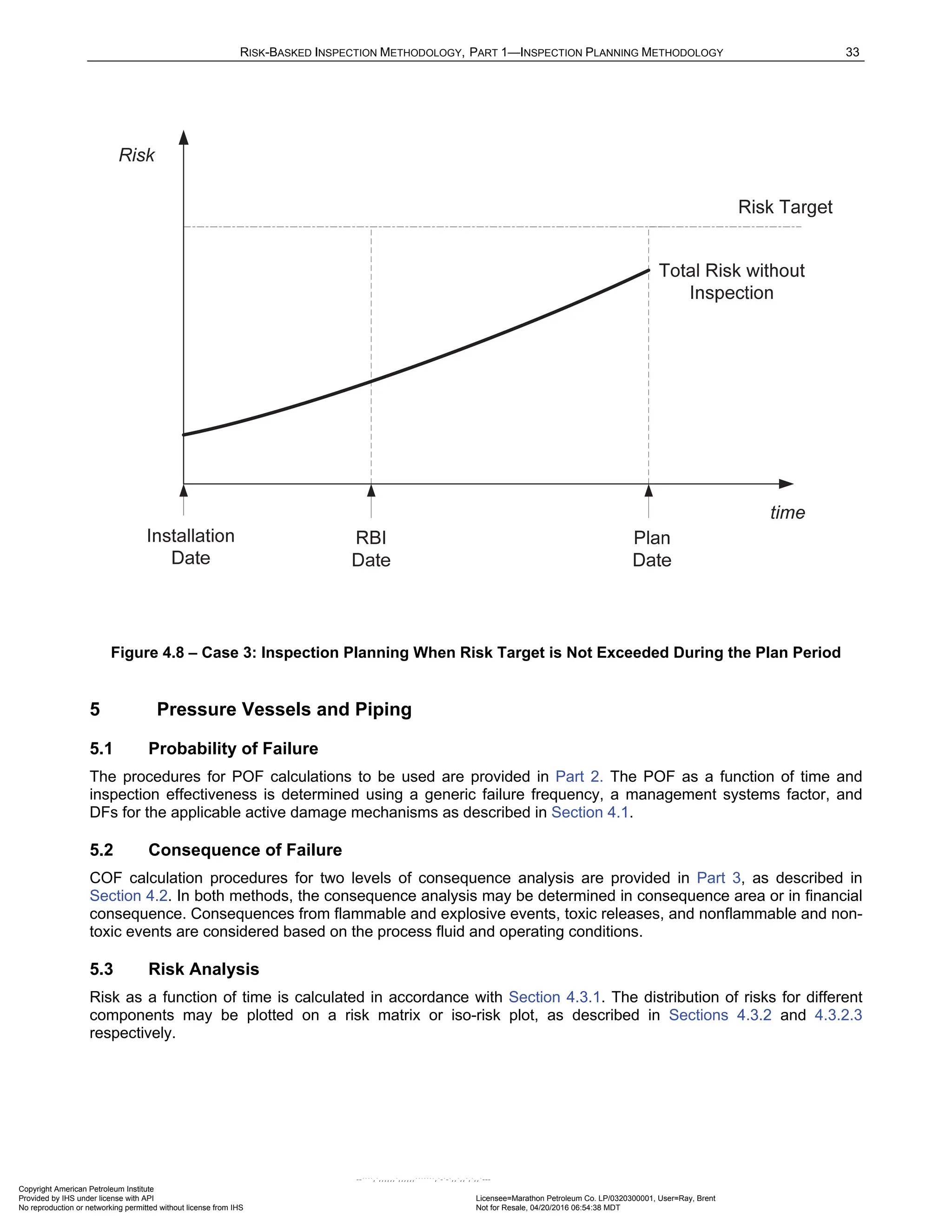
c) Case 3 – Risk at the Plan Date does not exceed the Risk Target – As shown in Figure 4.8, the risk at the
plan date does not exceed the risk target and therefore, no inspection is required during the plan period. In
this case, the inspection due date for inspection scheduling purposes may be set to the plan date so that
re-analysis of risk will be performed by the end of the plan period.
The concept of how the different inspection techniques with different effectiveness levels can reduce risk is
shown in Figure 4.6. In the example shown, a minimum of a B Level inspection was recommended at the target
date. This inspection level was sufficient since the risk predicted after the inspection was performed was
determined to be below the risk target at the plan date. Note that in Figure 4.6, a C Level inspection at the target
date would not have been sufficient to satisfy the risk target criteria.
4.5 Nomenclature
a is a variable provided for reference fluids for Level 1 COF analysis
n
A is the cross sectional hole area associated with the
th
n release hole size, mm2
(inch2
)
rt
A is the metal loss parameter
is the Weibull shape parameter
b is a variable provided for reference fluids for Level 1 COF analysis
f
C is the consequence of failure, m2
(ft2
) or , $
CA is the consequence impact area, m2
(ft2
)
flam
CA is the flammable consequence impact area, m2
(ft2
)
flam
n
CA is the flammable consequence impact area for each hole, m2
(ft2
)
( )
f
D t is the DF as a function of time, equal to f total
D − evaluated at a specific time
thin
f
D is the DF for thinning
f total
D − is total DF for POF calculation
MS
F is the management systems factor
FC is the financial consequence, $
gff is the generic failure frequency, failures/year
n
gff is the generic failure frequency for each of the n release hole sizes selected for the type of
equipment being evaluated, failures/year
total
gff is the sum of the individual release hole size generic frequencies, failures/year
is the Weibull characteristic life parameter, years
k is the release fluid ideal gas specific heat capacity ratio, dimensionless
s
P is the storage or normal operating pressure, kPa (psi)
( )
f
P t is the probability of failure as a function of time, failures/year
( )
,
f E
P t I is the probability of failure as a function of time and inspection effectiveness, failures/year
R is the universal gas constant = 8,314 J/(kg-mol)K [1545 ft-lbf/lb-mol°R]
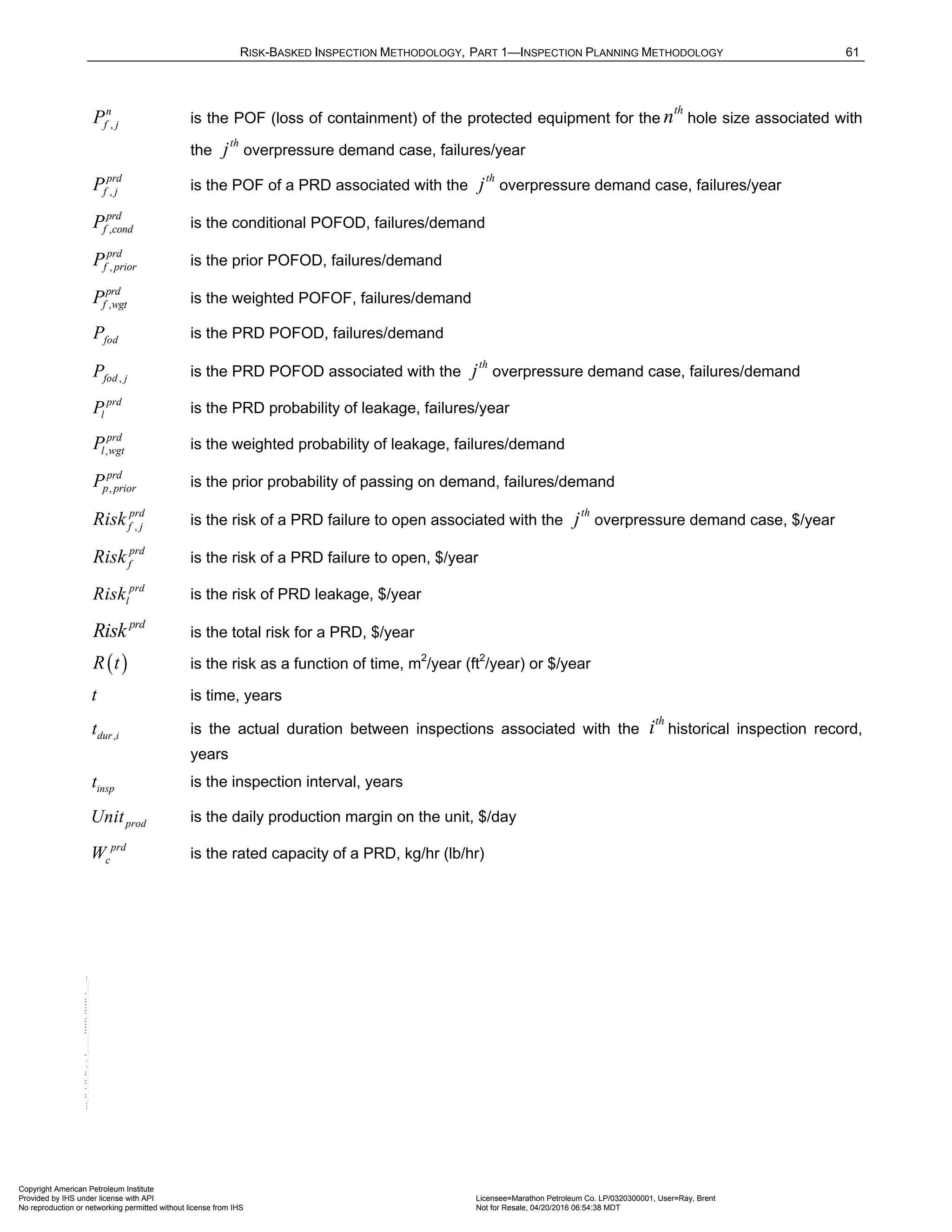
( )
R t is the risk as a function of time, m2
/year (ft2
/year) or $/year
( )
, E
R t I is the risk as a function of time and inspection effectiveness, m2
/year (ft2
/year) or $/year min
t
is the minimum required thickness, mm (inch)
X is the release rate or release mass for a Level 1 COF analysis, kg/s [lb/s] or kg [lb]
β
η
Copyright American Petroleum Institute
Provided by IHS under license with API Licensee=Marathon Petroleum Co. LP/0320300001, User=Ray, Brent
Not for Resale, 04/20/2016 06:54:38 MDT
No reproduction or networking permitted without license from IHS
--````,`,,,,,,`,,,,,,```````,`-`-`,,`,,`,`,,`---](https://image.slidesharecdn.com/api581-3rdedition-april2016-240227010601-3bf73ab5/75/Norma-API-581-3rd-Edition-April-2016-pdf-32-2048.jpg)
![34 API RECOMMENDED PRACTICE 581
5.4 Inspection Planning Based on Risk Analysis
The procedure to determine an inspection plan is provided in Section 4.4. This procedure may be used to
determine both the time and type of inspection to be performed based on the process fluid and design
conditions, component type and materials of construction, and the active damage mechanisms.
6 Atmospheric Storage Tanks
6.1 Probability of Failure
POF calculation procedures for AST shell courses and bottom plates are provided in Part 2. The POF as a
function of time and inspection effectiveness is determined using a generic failure frequency, a management
systems factor, and DFs for the applicable active damage mechanisms as described in Section 4.1. Typically,
the DFs for thinning in Part 2, Section 4 are used for AST components. However, DFs for other active damage
mechanisms may also be calculated using Part 2, Sections 4 through Section 24.
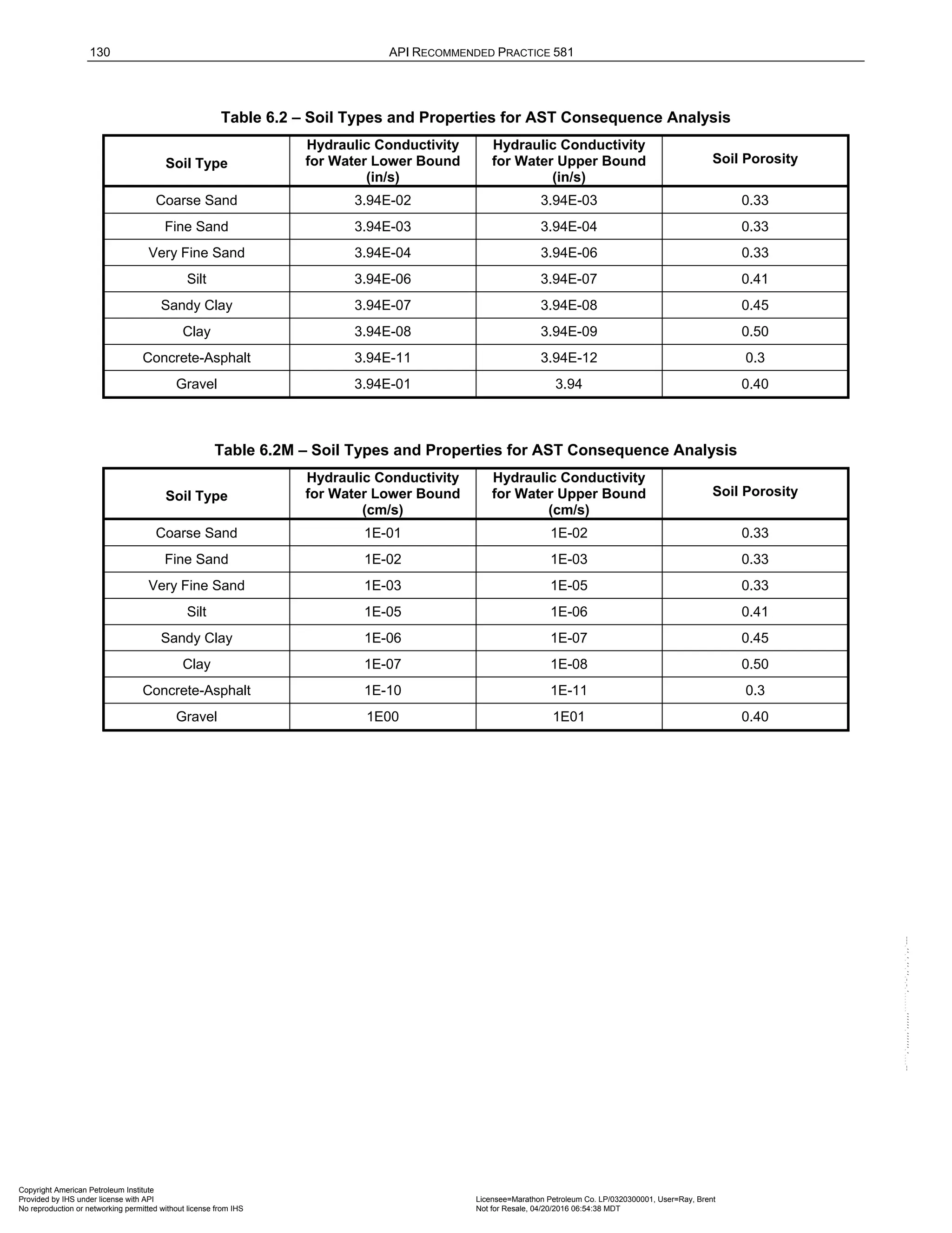
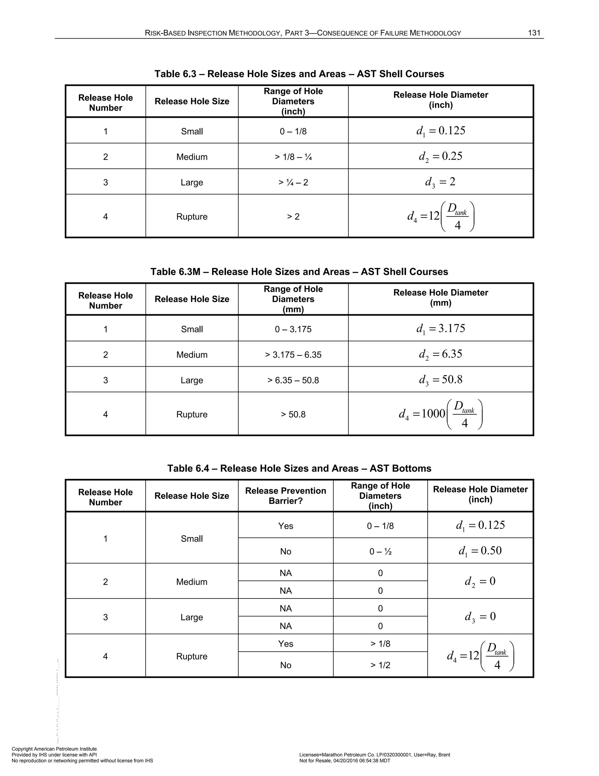
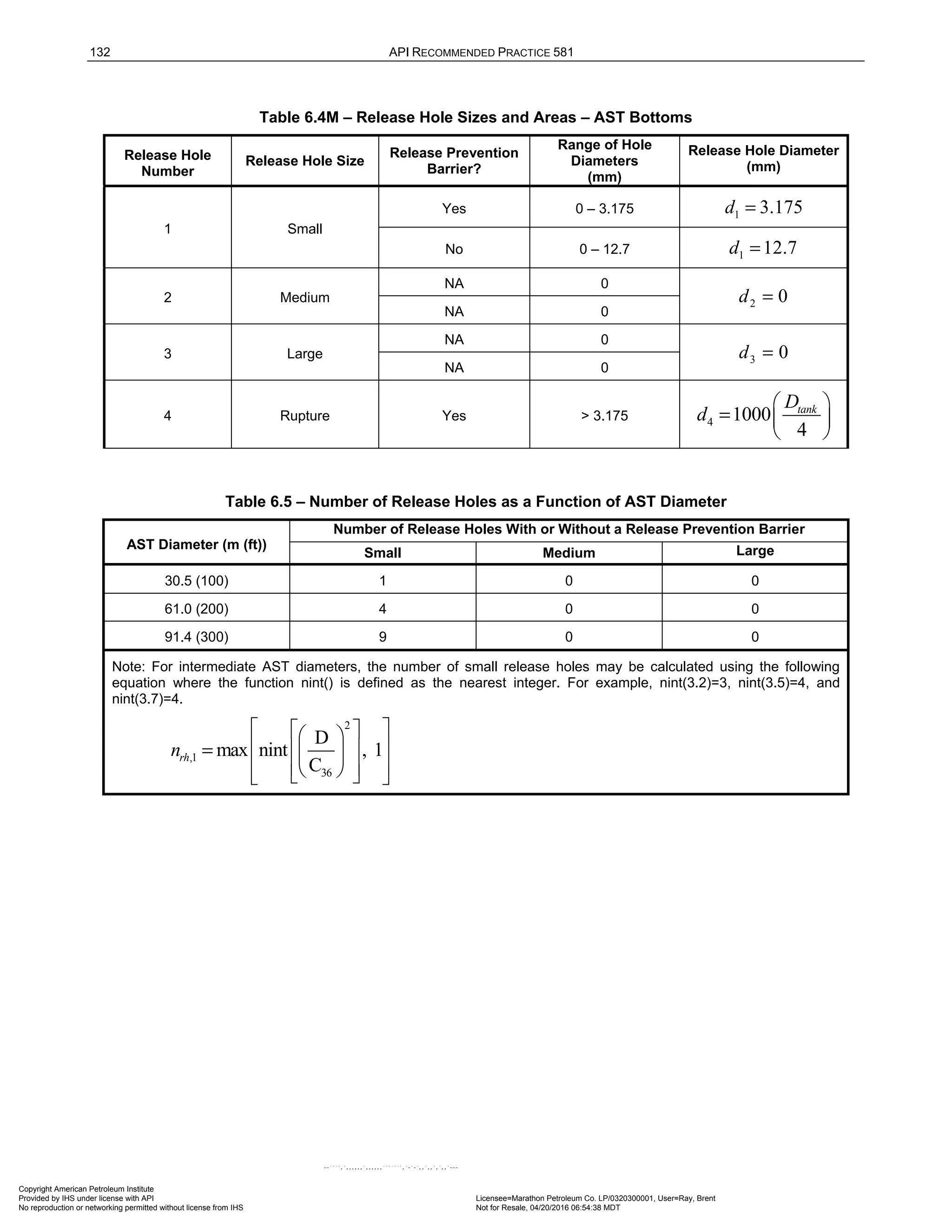
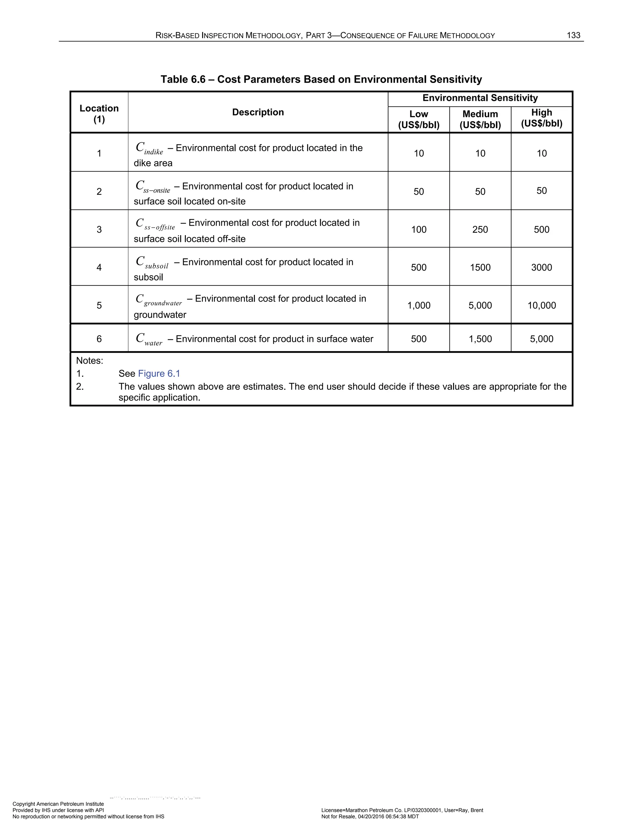
6.2 Consequence of Failure
COF calculation procedures for two levels of consequence analysis are provided in Part 3, Section 6. In both
methods, the COF may be determined in terms of consequence area or in financial consequence.
Consequences from flammable and explosive events, toxic releases, and nonflammable/nontoxic events are
considered in both methods based on the process fluid and operating conditions. Financial consequences from
component damage, product loss, financial impact, and environmental penalties are considered.
6.3 Risk Analysis
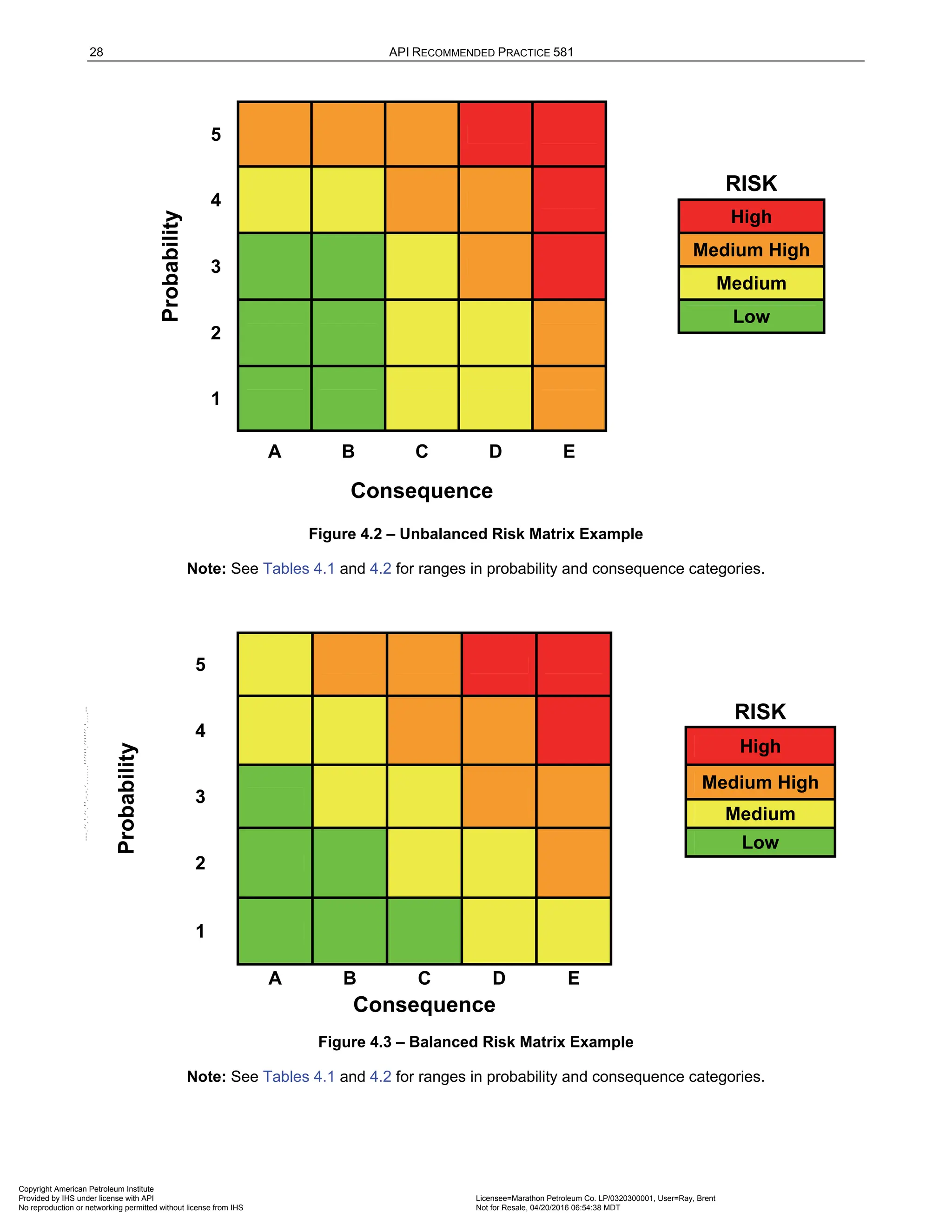
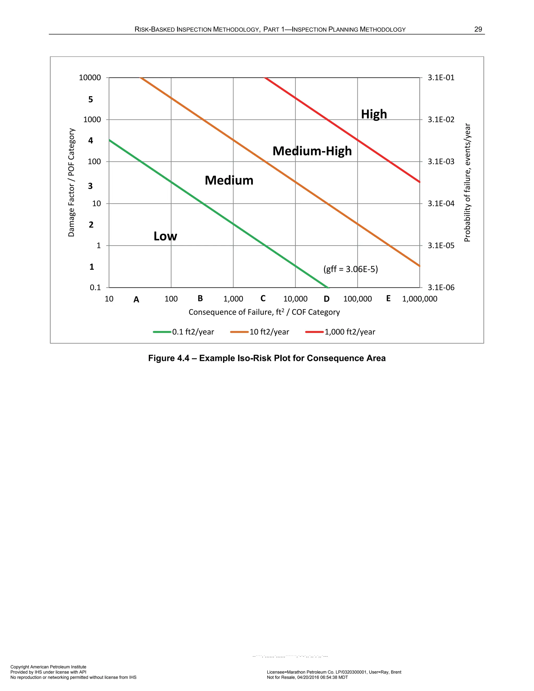
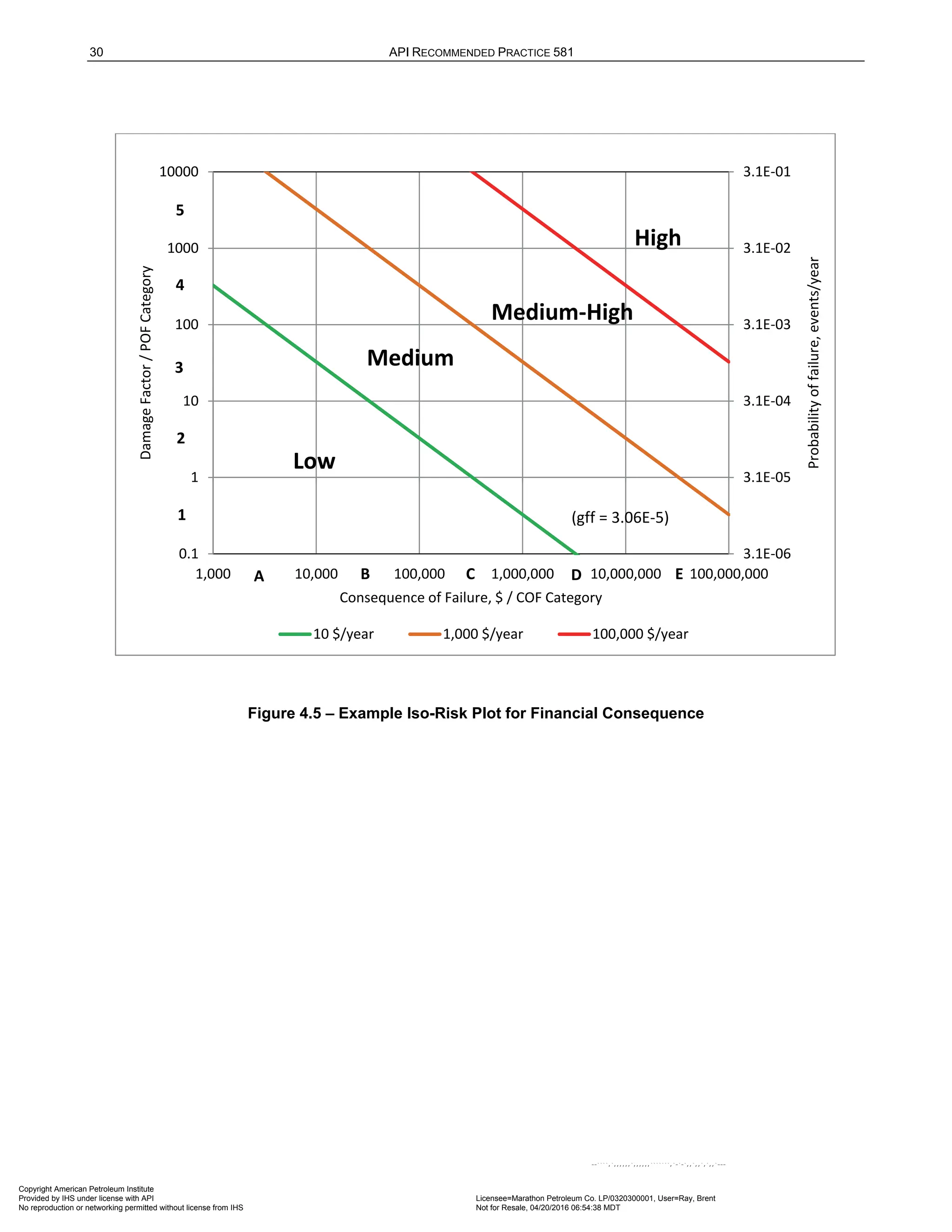
Risk as a function of time is calculated in accordance with Section 4.3.1. The distribution of risks for different
components may be plotted on a risk matrix or iso-risk plot, as described in Sections 4.3.2 and 4.3.2.3
respectively.
6.4 Inspection Planning Based on Risk Analysis
The procedure to determine an inspection plan is provided in Section 4.4. This procedure may be used to
determine both the time and type of inspection to be performed based on the process fluid and design
conditions, component type and materials of construction, and the active damage mechanisms.
7 Pressure Relief Devices
7.1 General
7.1.1 Overview
The major concern with PRDs and the main reason that routine PRD inspection and testing is required is that
the device may fail to relieve overpressure events that can cause failure of the equipment protected by the
device, leading to a loss of containment. There are also consequences associated with leakage of PRDs.
A risk-based approach to evaluating PRD criticality to set inspection/testing frequency is covered in this section.
Included in the scope are all spring-loaded and pilot-operated relief valves and rupture disks. Additional PRD
types, such as AST pressure/vacuum vents (P/V) and explosion hatches, may be analyzed provided reliability
data in the form of Weibull parameters exists for the PRD type being considered.
It is not the intention of the methodology for the user to perform or check PRD design or capacity calculations. It
is assumed that the owner-user has completed due diligence and the devices have been designed in
accordance with API 521 [11] and sized, selected, and installed in accordance with API 520 [12]. It is also
assumed that minimum inspection practices in accordance with API 576 [13] are in place.
Copyright American Petroleum Institute
Provided by IHS under license with API Licensee=Marathon Petroleum Co. LP/0320300001, User=Ray, Brent
Not for Resale, 04/20/2016 06:54:38 MDT
No reproduction or networking permitted without license from IHS
--````,`,,,,,,`,,,,,,```````,`-`-`,,`,,`,`,,`---](https://image.slidesharecdn.com/api581-3rdedition-april2016-240227010601-3bf73ab5/75/Norma-API-581-3rd-Edition-April-2016-pdf-42-2048.jpg)
![36 API RECOMMENDED PRACTICE 581
Using a two parameter Weibull distribution [14], the cumulative failure density function, ( )
F t , sometimes
referred to as Unreliability, is expressed in Equation (1.2) as shown in Section 4.1.3.
The Weibull η parameter or characteristic life is equivalent to the mean time to failure ( )
MTTF when the
Weibull β parameter is equal to 1.0. Throughout this document, discussions are made related to the
adjustment of the Weibull η parameter. Adjustments are made to the η parameter to increase or decrease the
POFOD and leakage either as a result of environmental factors, PRD types, or as a result of actual inspection
data for a particular PRD. These adjustments may be viewed as an adjustment to the mean time to failure
( )
MTTF for the PRD.
The assumption used to determine the default Weibull parameters is that PRDs in similar services will have a
similar POFOD, fod
P , and similar probability of leakage, l
P . Therefore, industry failure rate data may be used as
a basis for establishing the initial (or default) probabilities of failure for a specific device. The POFOD of the
specific device is related to identifiable process and installation conditions. Such conditions may include process
temperature, process corrosivity, and the tendency of the process to foul, polymerize, or otherwise block the
PRD inlet or prevent the PRD from reseating during operation. Also associated with failure are conditions such
as rough handling during transportation and installation and excessive piping vibration. Increased demand rates
and improper installations that result in chatter may also increase the POFOD and leakage.
7.1.5 PRD Testing, Inspection and Repair
Inspection, testing, reconditioning, or replacement of PRDs are recognized safe practices and serve to reduce
the POFOD and leakage. One of the key assumptions of the PRD methodology is that a bench test of a PRD
performed in the as-received condition from a process unit will result in a true determination of the performance
of the PRD on the unit.
A good inspection program for PRDs will track the history of inspection and testing of each PRD. Based on this
historical data, the PRD methodology will adjust the POF data for each PRD and allow for the varying degrees
of inspection effectiveness. Where a shop bench pre-pop test is performed, the resulting pass/fail data is given
the highest degree of confidence and the highest inspection effectiveness. Similarly, if a PRD is inspected and
overhauled without a pre-test, a lower confidence level or lower inspection effectiveness is associated with the
inspection.
7.1.6 PRD Overhaul or Replacement Start Date
When a PRD is overhauled in the shop, the basic assumption is made that the PRD is placed back into service
in an as-new condition. The original install date for the PRD remains the same, but the last inspection date is
changed to reflect the date that the PRD was overhauled. In this way, the calculated inspection interval and
subsequent new due date for the PRD is based on the last inspection date on which the PRD was overhauled.
When a PRD is replaced in lieu of overhaul, the install date and last inspection date are identical. The calculated
inspection interval and subsequent new due date for the PRD are based on the new install date.
Often PRDs are pop-tested either in the field or in the shop without overhauling the PRD. In these instances, the
PRD has not been returned to service in an as-new condition. Without an overhaul, the assumption is made that
the PRD remains in the condition that it was in prior to testing. In these cases, the POFOD for the device may
be adjusted based on the results of the field test (i.e., credit for inspection to reduce uncertainty), however, the
last overhaul date remains unchanged and therefore the PRD will not get the full benefit of an overhaul. In this
case, the due date is determined by adding the recommended inspection interval to the last overhaul date and
not the last inspection date.
7.1.7 Risk Ranking of PRDs
The PRD methodology allows a risk ranking to be made between individual PRDs and also allows a risk ranking
to be made between PRDs and other fixed equipment being evaluated.
Copyright American Petroleum Institute
Provided by IHS under license with API Licensee=Marathon Petroleum Co. LP/0320300001, User=Ray, Brent
Not for Resale, 04/20/2016 06:54:38 MDT
No reproduction or networking permitted without license from IHS
--````,`,,,,,,`,,,,,,```````,`-`-`,,`,,`,`,,`---](https://image.slidesharecdn.com/api581-3rdedition-april2016-240227010601-3bf73ab5/75/Norma-API-581-3rd-Edition-April-2016-pdf-44-2048.jpg)
![RISK-BASKED INSPECTION METHODOLOGY, PART 1—INSPECTION PLANNING METHODOLOGY 37
There are two key drivers for the effective risk ranking of PRDs with other PRDs. The first driver is in
establishing the specific reliability for each PRD. This may be accomplished by selecting the severity of service
of each PRD, establishing a default POF, and modifying the POFOD using the actual testing and inspection
history of each PRD. The second key driver is in the relative importance or criticality of each PRD. This is
accomplished through the relief system design basis and knowledge of the overpressure demand cases
applicable for each PRD. The more demand placed on a PRD and the more critical the PRD application, the
higher the risk ranking should be.
7.1.8 Link to Fixed or Protected Equipment
To effectively characterize the risk associated with PRD failure, the consequence associated with the failure of a
PRD to open upon demand must be tied directly to the equipment that the PRD protects. This is accomplished
using direct links to the fixed equipment RBI analysis as covered in Parts 2 and 3 of this document. The risk of
loss of containment from fixed equipment increases proportionately with the amount of overpressure that occurs
as a result of the PRD failing to open on demand. In addition, the calculated risk associated with damaged fixed
equipment will be greater than that for undamaged equipment since the actual damage states (i.e., DF, f
D ,
see Part 2) are used in the calculations.
Although consequences associated with PRD overpressure cases are greater than those associated with the
fixed equipment operating at normal pressure, this is tempered by the fact that the use of realistic PRD demand
rates and accurate PRD failure rate data results in a low frequency of occurrence.
7.2 Probability of Failure (FAIL)
7.2.1 Definition
For a PRD, it is important that the definition of failure be understood, since it is different than failure of other
equipment types. A PRD failure is defined as failure to open during emergency situations causing an
overpressure situation in the protected equipment, resulting in loss of containment (failures/year). Leakage
through a PRD is also a failure. This type of failure is discussed in Section 7.3.
7.2.2 Calculation of Probability of Failure to Open
The fundamental calculation applied to PRDs for the fail to open case is the product of an estimated
overpressure demand case frequency (or demand rate), the probability of the PRD failing to open on demand,
and the probability that the protected equipment at higher overpressures will lose containment.
A PRD protects equipment components from multiple overpressure scenarios. Guidance on overpressure
demand cases and pressure relieving system design is provided in API 521 [11]. Each of these scenarios (fire,
blocked discharge, etc.) can result in a different overpressure, ,
o j
P , if the PRD were to fail to open upon
demand. Additionally, each overpressure scenario has its own demand rate, j
DR . Demand cases are discussed
in more detail in Section 7.4.3 and Table 7.2 and Table 7. 3. The expression for POF for a PRD for a particular
overpressure demand case is as shown in Equation (1.11).
, , ,
prd
f j fod j j f j
P P DR P
= ⋅ ⋅ (1.11)
The subscript j in the above equation indicates that the POF for the PRD, ,
prd
f j
P , needs to be calculated for
each of the applicable overpressure demand cases associated with the PRD.
The POF (loss of containment) of the equipment component that is protected by the PRD, ,
f j
P , is a function of
time and the potential overpressure. API RP 581 recognizes that there is an increase in probability of loss of
containment from the protected equipment due to the elevated overpressure if the PRD fails to open during an
emergency event.
Each of the terms that make up the POF for the PRD shown in Equation (1.11) is discussed in greater detail in
the following sections.
a) Section 7.2.3 – PRD Demand Rate, j
DR
Copyright American Petroleum Institute
Provided by IHS under license with API Licensee=Marathon Petroleum Co. LP/0320300001, User=Ray, Brent
Not for Resale, 04/20/2016 06:54:38 MDT
No reproduction or networking permitted without license from IHS
--````,`,,,,,,`,,,,,,```````,`-`-`,,`,,`,`,,`---](https://image.slidesharecdn.com/api581-3rdedition-april2016-240227010601-3bf73ab5/75/Norma-API-581-3rd-Edition-April-2016-pdf-45-2048.jpg)
![38 API RECOMMENDED PRACTICE 581
b) Section 7.2.4 – PRD POFOD, ,
fod j
P
c) Section 7.2.5 – POF of Protected Equipment as a Result of Overpressure , ,
f j
P
7.2.3 PRD Demand Rate
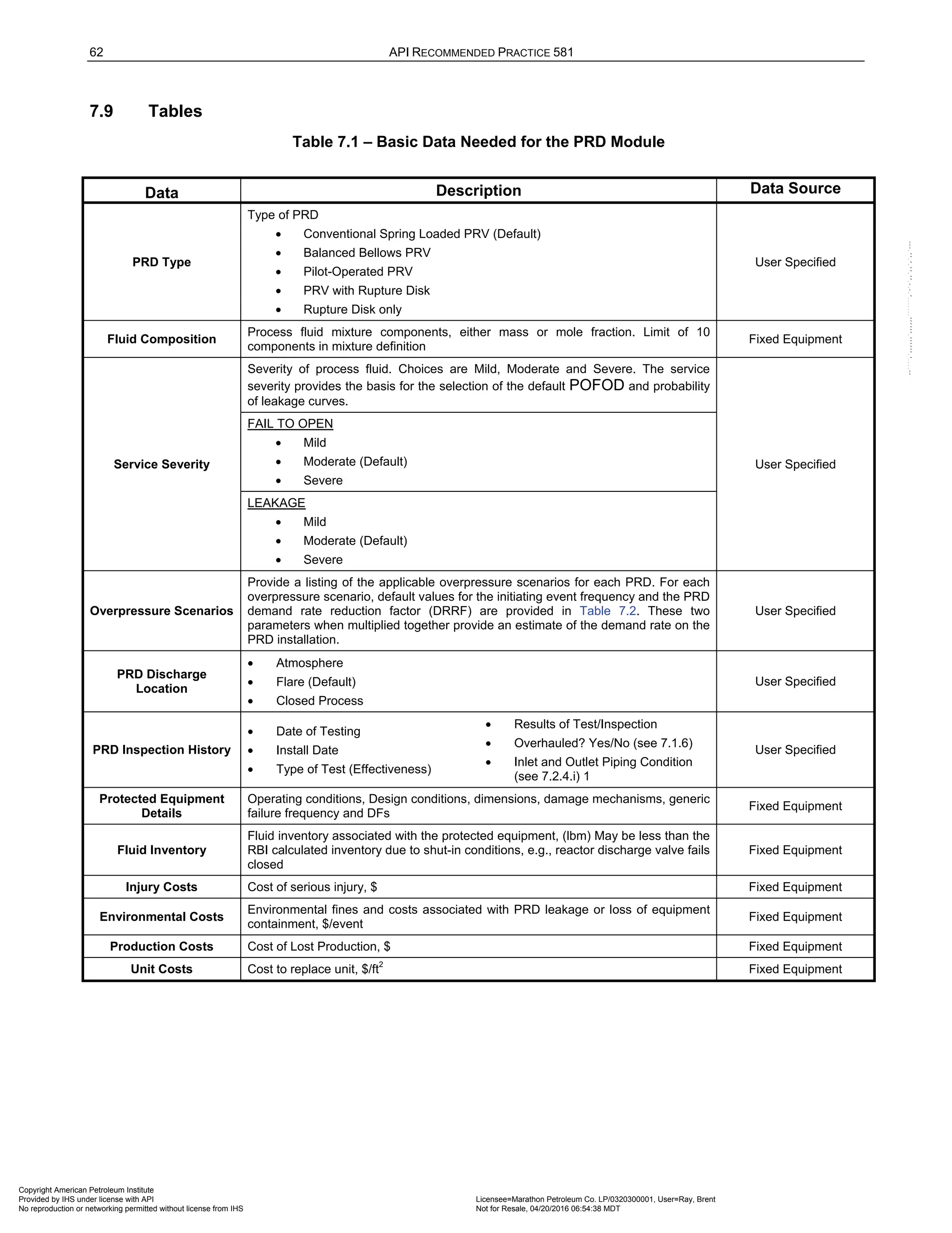
a) Default Initiating Event Frequencies
The first step in evaluating the probability of a PRD failure is to determine the demand rate (demands or
events/year) placed on the device. API RP 581 provides estimates for the PRD initiating event frequencies,
j
EF based on the various relief overpressure demand cases that the device is providing protection.
Examples of the initiating event frequencies are provided in Table 7.2. Additional background on the default
initiating event frequencies is provided in Table 7. 3.
b) Credit for Other Layers of Protection
It is recognized that the actual demand rate on a PRD is not necessarily equal to the initiating event
frequency. The concept of a demand rate reduction factor, j
DRRF , is introduced here to account for the
difference in the overpressure demand case event frequency and the demand rate on the PRD.
Many pressure vessel installations include control systems, high integrity protective instrumentation,
shutdown systems, and other layers of protection to reduce the demand rate of a PRD. Credit can be taken
for operator intervention to reduce the probability of overpressure.
The j
DRRF is used to account for these additional layers of protection. The j
DRRF may be determined
rigorously for the installation as a result of a layer of protection analysis (LOPA).
Another example of where credit may be taken using the j
DRRF is for the fire overpressure demand case.
A good estimate for the initiating event frequency of a fire on a specific pressure vessel is 1 every 250
years (0.004 events/year). However, due to many other factors, fire impingement from a pool directly on a
pressure vessel rarely causes the pressure in the vessel to rise significantly enough to cause the PRD to
open. Factors reducing the actual demand rate on the PRD include fire proofing, availability of other
escape paths for the process fluid, and fire-fighting efforts at the facility (to reduce the likelihood of
overpressure).
c) Calculation of Demand Rate (DR)
The demand rate (DR) on the PRD is calculated as the product of the initiating event frequency and the
j
DRRF in accordance with Equation (1.12):
j j j
DR EF DRRF
= ⋅ (1.12)
The subscript j in Equation (1.12) signifies that the demand rate on a PRD is calculated for each
applicable overpressure demand case.
Typically, a PRD protects equipment for several overpressure demand cases and each overpressure case
has a unique demand rate. Default initiating event frequencies for each of the overpressure cases are
provided inTable 7.2. Additional guidance on overpressure demand cases and pressure relieving system
design is provided in API 521 [11]. An overall demand rate on the PRD can be calculated in
Equation (1.13):
1
ndc
total j
j
DR DR
=
= (1.13)
If the relief design basis of the PRD installation has not been completed, the list of applicable overpressure
demand cases may not be available and it may be more appropriate to use a simple overall average value
of the demand rate for a PRD. An overall demand rate for a particular PRD can usually be estimated from
past operating experience for the PRD.
Copyright American Petroleum Institute
Provided by IHS under license with API Licensee=Marathon Petroleum Co. LP/0320300001, User=Ray, Brent
Not for Resale, 04/20/2016 06:54:38 MDT
No reproduction or networking permitted without license from IHS
--````,`,,,,,,`,,,,,,```````,`-`-`,,`,,`,`,,`---](https://image.slidesharecdn.com/api581-3rdedition-april2016-240227010601-3bf73ab5/75/Norma-API-581-3rd-Edition-April-2016-pdf-46-2048.jpg)
![RISK-BASKED INSPECTION METHODOLOGY, PART 1—INSPECTION PLANNING METHODOLOGY 41
3) Use of Plant-Specific Failure Data
Data collected from specific plant testing programs can also be used to obtain POFOD and probability of
leakage values. Different measures such as MTTF or failure per million operating hours may be
converted into the desired form via simple conversion routines.
d) Default Data for Balanced Bellows Pressure Relief Valves
A balanced spring-loaded PRV uses a bellows to isolate the back side of the disk from the effects of
superimposed and built-up back pressure. The bellows also isolates the internals of the PRD from the
corrosive effects of the fluid in the discharge system.
An analysis of industry failure rate data shows that balanced bellows PRVs have the same POFOD rates
as their conventional PRD counterparts, even though they typically discharge to dirty/corrosive closed
systems. This is due to the isolation of the valve internals from the discharge fluid and the effects of
corrosion and fouling. As shown in Table 7.5, the characteristic life (Weibull η parameter) is the same for
bellows PRVs as it is for conventional PRVs.
e) Default Weibull Parameters for Pilot-Operated Pressure Relief Valves
To date, there is little failure rate data in the industry available for pilot-operated PRVs. One source [15]
indicates that pilot-operated PRVs are 20 times more likely to fail than their spring-loaded counterparts.
The Weibull parameters for the POFOD curves for conventional PRVs as shown in Table 7.5 are used as
the basis for pilot-operated PRVs with adjustment factors applied to the characteristic life (η parameter).
For MILD service, the η parameter for pilot-operated PRVs is reduced by a factor of 1.5; for MODERATE
service, the reduction factor is 3.0; and for SEVERE service, the reduction factor is 5.0.
f) Default Weibull Parameters for Rupture Disks
To date, there is little failure rate data in the industry available for rupture disks. Rupture disks are simple,
reliable devices that are not likely to fail to open at pressures significantly over their burst pressure (unless
inlet or outlet plugging is a problem, or unless they are installed improperly). Typically, if a rupture disk
were to fail, it would burst early. Therefore, the Weibull parameters for the failure to open upon demand
case for rupture disks are based on the MILD severity curve for conventional PRVs. This makes the
assumption that a rupture disk is at least as reliable as a conventional PRV. It also assumes that the
rupture disk material has been properly selected to withstand the corrosive potential of the operating fluid.
Where it is known that the rupture disk material is not properly selected for the corrosive service, the disk
Weibull parameters should be adjusted accordingly.
g) Adjustment for Conventional PRVs Discharging to Closed System
An adjustment is made to the base Weibull parameters for conventional valves that discharge to a closed
system or to flare. Since a conventional valve does not have a bellows to protect the bonnet housing from
the corrosive fluids in the discharge system, the characteristic life (represented by the η parameter) is
reduced by 25%, using an adjustment factor of 0.75.
c
F = 0.75 for conventional valves discharging to closed system or flare
c
F =1.0 for all other cases
h) Adjustment for Environmental Factors
There are several environmental and installation factors that can affect the reliability of PRDs. These
include the existence of vibration in the installed piping, a history of chatter, and whether or not the device
is located in pulsing flow or cyclical service, such as when the device is installed downstream of
reciprocating rotating equipment. Other environmental factors that can significantly affect leakage
probability are operating temperature and operating ratio.
Copyright American Petroleum Institute
Provided by IHS under license with API Licensee=Marathon Petroleum Co. LP/0320300001, User=Ray, Brent
Not for Resale, 04/20/2016 06:54:38 MDT
No reproduction or networking permitted without license from IHS
--````,`,,,,,,`,,,,,,```````,`-`-`,,`,,`,`,,`---](https://image.slidesharecdn.com/api581-3rdedition-april2016-240227010601-3bf73ab5/75/Norma-API-581-3rd-Edition-April-2016-pdf-49-2048.jpg)
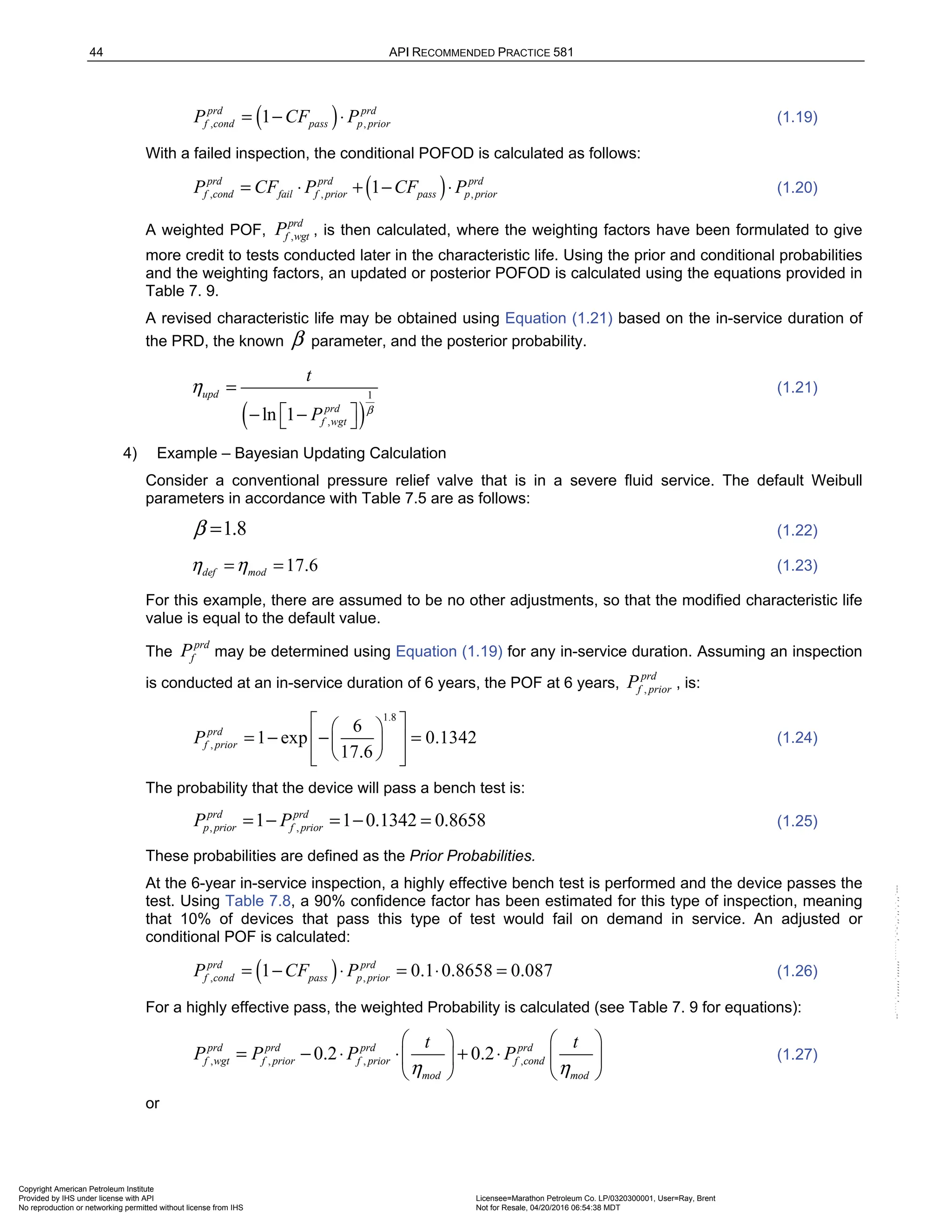
![RISK-BASKED INSPECTION METHODOLOGY, PART 1—INSPECTION PLANNING METHODOLOGY 45
( )
,
6 6
0.1342 0.2 0.1342 0.2 0.087 0.1310
17.6 17.6
prd
f wgt
P
= − ⋅ ⋅ + ⋅ ⋅ =
(1.28)
Finally, using the prior β and the calculated weighted probability, ,
prd
f wgt
P , an updated value for the η
parameter is calculated for the in-service duration using Equation (1.29).
( )
1
,
ln 1
upd
prd
f wgt
t
P β
η =
− −
(1.29)
or
[ ]
( )
1
1.8
6
17.9
ln 1 0.1310
upd
η = =
− −
(1.30)
The weighting factors assure a gradual shift from default POFOD data to field POFOD data, and do not
allow the characteristic life to adjust upward too rapidly. They will, however, shorten characteristic life if
the device has repeated failures early in its service.
Other points that are not accounted for in the calculation procedure regarding inspection updating:
i) Tests conducted at less than one year do not get credit.
ii) After a pass, the characteristic life cannot decrease. If the procedure yields a decrease in
characteristic life, this value should not be used. The characteristic life should be kept equal to
the previous value.
iii) After a fail, the characteristic life cannot increase. If the procedure yields an increase in
characteristic life, this value should not be used. The characteristic life should be kept equal to
the previous value.
5) Updating Failure Rates after Modification to the Design of the PRD
Design changes are often made to PRDs that improve the reliability of the device and result in a change
in the failure rate, for example upgrading to a corrosion resistant material or installation of an upstream
rupture disk. Past inspection data is no longer applicable to the newly designed installation. In these
cases, either a new default curve should be selected per Figure 7.2 or device specific Weibull
parameters should be chosen based on owner-user experience, thus generating a unique curve for the
device.
j) Adjustment for Overpressures Higher than Set Pressure
As discussed in Section 7.1.3, the POFOD curves are based on bench test data where a failure is defined
as any test requiring a pressure greater than 1.3 times the set pressure. Intuitively, one would expect that
at higher overpressures, the probability that the PRD would fail to open goes down dramatically. A review
of the industry failure data supports this. Figure 7.4 shows that as the overpressure ratio increases, the
PRD failure rate reduces significantly.
A conservative approach is to assume that the failure rate is cut by a factor of 5 at 4.0 times the set
pressure and to assume linear interpolation between 1.3 and 4.0 times the set pressure. A factor for
overpressure, , is introduced in Equation (1.31).
op
F
Copyright American Petroleum Institute
Provided by IHS under license with API Licensee=Marathon Petroleum Co. LP/0320300001, User=Ray, Brent
Not for Resale, 04/20/2016 06:54:38 MDT
No reproduction or networking permitted without license from IHS
--````,`,,,,,,`,,,,,,```````,`-`-`,,`,,`,`,,`---](https://image.slidesharecdn.com/api581-3rdedition-april2016-240227010601-3bf73ab5/75/Norma-API-581-3rd-Edition-April-2016-pdf-53-2048.jpg)
![46 API RECOMMENDED PRACTICE 581
,
,
,
,
,
,
1.0 1.3
0.2 4.0
1
1 1.3
3.375
o j
OP j
set
o j
OP j
set
o j
OP j
set
P
F for
P
P
F for
P
P
F for all other cases
P
= <
= >
= − ⋅ −
(1.31)
The adjustment factor calculated above cannot be less than 0.2, nor greater than 1.0.
7.2.5 Protected Equipment Failure Frequency as a Result of Overpressure
a) General
Where risk analysis has been completed for equipment components being protected by PRDs, each piece
of protected equipment has a damage adjusted failure frequency computed as the equipment’s generic
failure frequency multiplied by a DF, see Section 4.1 and Equation (1.1). The DF is determined based on
the applicable damage mechanisms for the equipment, the inspection history and condition of the
equipment. In The DFs for the protected equipment are calculated as a function of time. This is very
important when evaluating the inspection interval for the PRD. As the PRD inspection interval is extended,
the damage related to the vessel increases as does the risk associated with the PRD.
The damage adjusted failure frequencies are calculated at the normal operating pressure of the equipment
and are adjusted when evaluating PRDs as follows. When a PRD fails to open upon demand, the pressure
in the protected equipment rises above the operating pressure and in many cases, significantly above the
MAWP. The protected equipment damage adjusted failure frequency [ ( )
f
P t from Equation (1.1)] is
adjusted based on the calculated overpressure for the overpressure demand case under consideration.
The damage adjusted failure frequency, which is equal to the probability of loss of containment from the
protected equipment, at the overpressure is calculated as follows:
( )
,
3.464837
, 0.0312881
o j
P
MAWP
f j total f MS
P gff D F e
⋅
= ⋅ ⋅ ⋅ ⋅ (1.32)
The above equation is set up so that at normal operating pressure ( MAWP
≤ ), the probability of loss of
containment from the equipment, ,
f j
P , is equal to the damage adjust failure frequency, f
P , calculated in
fixed equipment RBI for the protected equipment using Equation (1.1). At elevated overpressures when the
PRD is being evaluated, the probability of loss of containment in the protected equipment increases. As an
upper limit, for an undamaged piece of equipment ( 1.0
f
D = ), the probability of loss of containment will
equal 1.0 when the overpressure is equal to 4 times the maximum allowable working pressure (MAWP).
For a damaged piece of equipment ( 1.0
f
D ), the probability of loss of containment can reach 1.0 at
pressures much lower than 4 times the MAWP , see Figure 7.6 for further clarification.
The probability of occurrence of any of the four holes sizes (i.e. small leak to rupture) is increased at
elevated overpressures due to the increased probability of loss of containment and may be calculated as
follows:
, ,
n n
f j f j
total
gff
P P
gff
=
(1.33)
See Part 1, Section 4.2.2 for initial discussion on the discrete hole sizes, Part 2, Table 3.1 for gff and
total
gff and Part 3 Table 4.4 for definitions of the hole and actual representative sizes.
Copyright American Petroleum Institute
Provided by IHS under license with API Licensee=Marathon Petroleum Co. LP/0320300001, User=Ray, Brent
Not for Resale, 04/20/2016 06:54:38 MDT
No reproduction or networking permitted without license from IHS
--````,`,,,,,,`,,,,,,```````,`-`-`,,`,,`,`,,`---](https://image.slidesharecdn.com/api581-3rdedition-april2016-240227010601-3bf73ab5/75/Norma-API-581-3rd-Edition-April-2016-pdf-54-2048.jpg)
![RISK-BASKED INSPECTION METHODOLOGY, PART 1—INSPECTION PLANNING METHODOLOGY 53
This multiple device installation factor reduces the potential overpressure that is likely to occur by assuming that
some of the installed PRD relief area will be available if the PRD under consideration fails to open upon
demand. The multiple device installation adjustment factor has a minimum reduction value of 0.25. The
presence of the square root takes into consideration that the PRDs in a multiple device installation may have
common failure modes. The reduction in overpressure as a result of multiple PRDs is in accordance with
Equation (1.38):
, ,
o j a o j
P F P
= ⋅ (1.38)
The multiple installation adjustment factor, a
F , is a ratio of the area of a single PRD (being analyzed) to the
overall areas of all PRDs in the multiple setup.
This reduced overpressure should be implemented when determining the protected equipment failure
frequency. However, it should not be considered when determining the overpressure factor, OP
F , which is used
to determine the POFOD in Section 7.2.4.i.
7.4.5 Calculation of Consequence of Failure to Open
Consequence calculations are performed for each overpressure demand case that is applicable to the PRD.
These consequence calculations are described in Part 3 of this document for each piece of equipment that is
protected by the PRD being evaluated and are performed at higher potential overpressures as described in
Section 7.4.1.
The overpressure for each demand case that may result from a failure of a PRD to open upon demand has two
effects. The probability of loss of containment from the protected equipment can go up significantly as discussed
in Section 7.2.5. Secondly, the consequence of failure as a result of the higher overpressures also increases.
The magnitude of the release increases in proportion to the overpressure, thus increasing the consequence of
events such as jet fires, pool fires, and vapor cloud explosions. Additionally, the amount of explosive energy
released as a result of a vessel rupture increases in proportion to the amount of overpressure. Part 3 provides
detail for the consequences associated with loss of containment from equipment components.
The consequence calculations should be performed in accordance with Part 3 for each of the overpressure
demand cases applicable to the PRD and for each piece of equipment that is protected by the PRD. The
resultant consequence is ,
prd
f j
C expressed in financial terms, ($/yr).
7.4.6 Calculation Procedure
The following procedure may be used to determine the consequence of a PRD failure to open.
a) STEP 1 – Determine the list of overpressure scenarios applicable to the piece of equipment being
protected by the PRD under evaluation. Table 7.2 provides a list of overpressure demand cases specifically
covered. Additional guidance on overpressure demand cases and pressure relieving system design is
provided in API 521 [11].
b) STEP 2 – For each overpressure demand case, estimate the amount of overpressure, ,
o j
P , likely to occur
during the overpressure event if the PRD were to fail to open. Section 7.4.3 and Table 7. 3 provide
guidance in this area.
c) STEP 3 – For installations that have multiple PRDs, determine the total amount of installed PRD orifice
area,
prd
total
A , including the area of the PRD being evaluated. Calculate the overpressure adjustment factor,
a
F , in accordance with Equation (1.37).
d) STEP 4 – Reduce the overpressures determined in STEP 3 by the overpressure adjustment factor in
accordance with Equation (1.38).
e) STEP 5 – For each overpressure demand case, calculate the financial consequence, ,
prd
f j
C , of loss of
containment from the protected equipment using procedures developed in Part 3. Use the overpressures
for the demand cases as determined in STEP 4 in lieu of the operating pressure, s
P .
Copyright American Petroleum Institute
Provided by IHS under license with API Licensee=Marathon Petroleum Co. LP/0320300001, User=Ray, Brent
Not for Resale, 04/20/2016 06:54:38 MDT
No reproduction or networking permitted without license from IHS
--````,`,,,,,,`,,,,,,```````,`-`-`,,`,,`,`,,`---](https://image.slidesharecdn.com/api581-3rdedition-april2016-240227010601-3bf73ab5/75/Norma-API-581-3rd-Edition-April-2016-pdf-61-2048.jpg)
![54 API RECOMMENDED PRACTICE 581
f) STEP 6 – Using the values as determined above, refer to Section 7.6 to calculate the risk.
7.5 Consequence of Leakage
7.5.1 General
Even though the consequences of PRD leakage are typically much less severe than that of a loss of
containment from the protected equipment as a result of a PRD failure to open, the frequency of leakage may
be high enough that the PRD may be ranked as a high priority on a leakage risk basis.
The calculation of leakage consequence from PRDs,
prd
l
C , is estimated by summing the costs of several items.
The cost of the lost inventory is based on the cost of fluid multiplied by the leakage rate (see
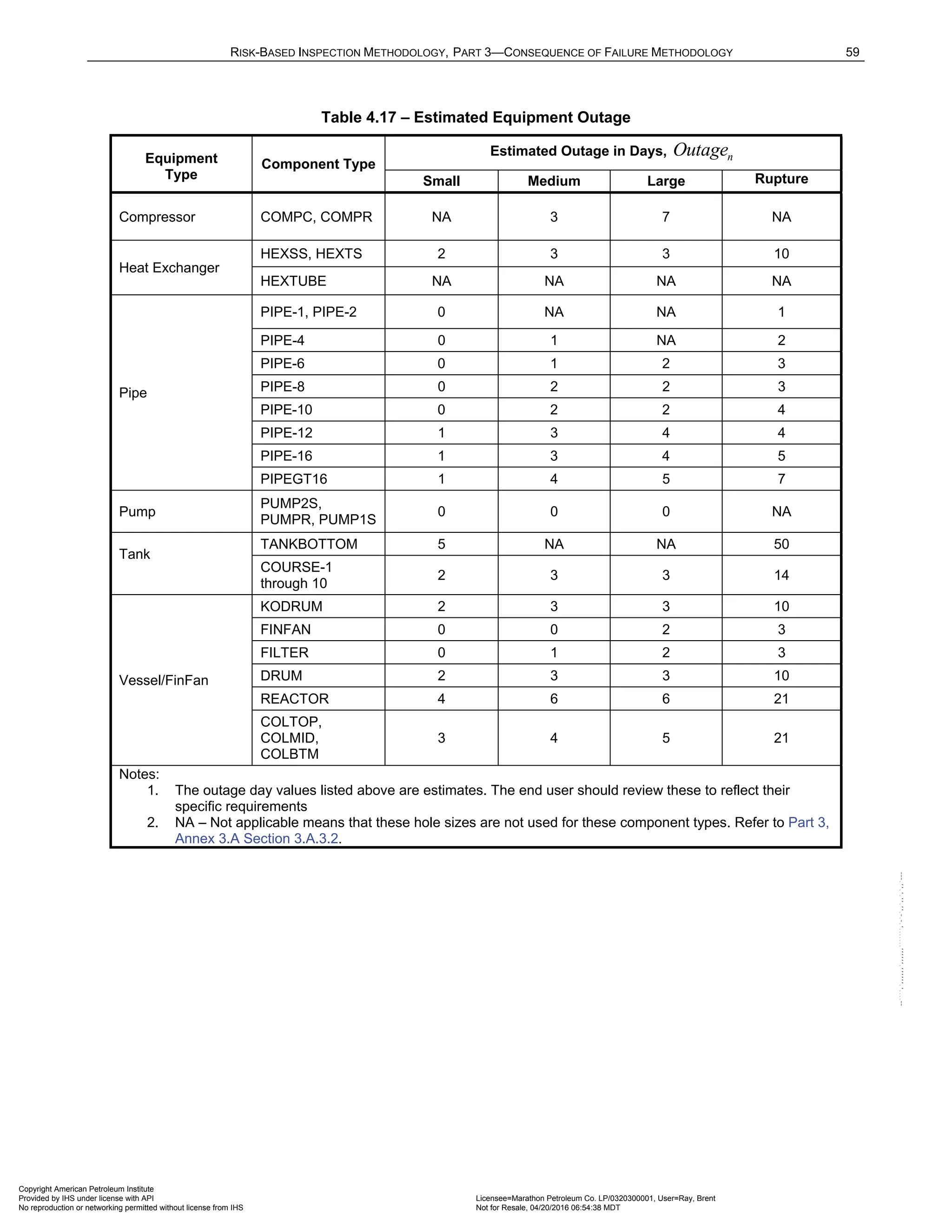
Section 7.5.5.) and the number of days to discover the leak (see Table 7.14). Regulatory and environmental
costs associated with leakage should be considered as well. Next, the cost of downtime to repair or replace the
device is estimated if it is determined that continuous operation of the unit with a leaking or stuck open PRD
cannot be tolerated. If a shutdown is required to repair the leaking PRD, then the cost associated with lost
production will also be added.
The consequence of leakage,
prd
l
C , is calculated using the following equation:
prd
l inv env sd prod
C Cost Cost Cost Cost
= + + + (1.39)
For a multiple device installation, the probability of leakage for any one specific PRD does not increase.
However, since the number of devices increases, the probability of a leak and its associated consequences
does increase in proportion to the number of devices protecting the system.
7.5.2 Estimation of PRD Leakage Rate
An analysis of industry bench test data shows that approximately 8.4% of the PRVs tested had some leakage
on the bench stand between 70% and 90% of their set pressure. An additional 6.6% of the PRVs tested leaked
at pressures below 70% of their set pressure. An additional 2.4% of the tested PRVs leaked significantly below
70% of their set pressure. The basis for the estimated leakage rates used for the consequence calculation is
provided in Table 7.15.
As shown in Table 7.15, a leakage rate of 1% of the PRD capacity (calculated at normal operating conditions) is
used for mild and moderate leaks. For a stuck open PRD, the leakage rate is assumed to be 25% of the PRD
capacity, as given in Equation (1.41).
Two leak cases are evaluated. The first case handles minor or moderate leakage,
mild
l
C , and represents 90% of
all of the potential leakage cases, per Table 7.15. A stuck open case results in a leakage consequence,
so
l
C ,
and makes up 10% of all possible leakage cases.
For mild and moderate leaks, 1% of the rated capacity of the PRD,
prd
c
W , is the basis for the leakage rate, see
Equation (1.40).
0.01 prd
mild c
lrate W
= ⋅ (1.40)
For the stuck open or spurious open case, the leakage rate is estimated per Equation (1.41).
0.25 prd
so c
lrate W
= ⋅ (1.41)
The rated capacity of the PRD,
prd
c
W , can usually be found on the PRD data sheet. It can also be calculated
using the methods presented in API 520 Part 1 [12].
Copyright American Petroleum Institute
Provided by IHS under license with API Licensee=Marathon Petroleum Co. LP/0320300001, User=Ray, Brent
Not for Resale, 04/20/2016 06:54:38 MDT
No reproduction or networking permitted without license from IHS
--````,`,,,,,,`,,,,,,```````,`-`-`,,`,,`,`,,`---](https://image.slidesharecdn.com/api581-3rdedition-april2016-240227010601-3bf73ab5/75/Norma-API-581-3rd-Edition-April-2016-pdf-62-2048.jpg)
![56 API RECOMMENDED PRACTICE 581
0.0
mild
prod
Cost if a leaking PRD can betolerated or if the PRD can
be isolated and repaired without requiring a shutdown
=
(1.45)
mild
prod prod sd
Cost Unit D if a leaking PRD cannot be tolerated
= ⋅ (1.46)
so
prod prod sd
C Unit D for a stuck open PRD
= ⋅ (1.47)
7.5.9 Calculation of Leakage Consequence
The consequence of leakage is calculated for two leaks cases.
a) Mild to Moderate Leakage
The first case handles minor or moderate leakage, ,
prd
l leak
C , and is used to represent 90% of all of the
potential leakage cases, per Table 7.15. In this case, the leakage rate is 1% of the PRD capacity and the
duration (or time to discover the leak) is a function of PRD inlet size and discharge location as shown in
Table 7.14.
mild mild mild
l inv env sd prod
C C C C C
= + + + (1.48)
b) Stuck Open Leakage
The second case handles the stuck open leak case, ,
prd
l so
C , and is assumed to have a duration of 30
minutes. In this case, to determine the cost of lost fluid, 25% of the full capacity of the PRD (calculated at
normal operating conditions) is used for the leakage rate and it is assumed that the PRD will be repaired
immediately (within 30 minutes).
so so so
l inv env sd prod
C C C C C
= + + + (1.49)
c) Final Leakage Consequence
The final leakage consequence is calculated using Equation (1.50) and is weighted based on the how likely
each of the cases is to occur as follows:
0.9 0.1
prd mild so
l l l
C C C
= ⋅ + ⋅ (1.50)
7.5.10 Calculation Procedure
The following procedure may be used to determine the consequence of leakage from a PRD.
a) STEP 1 – Determine the flow capacity of the PRD,
prd
c
W . This can be taken from the PRD data sheet or
calculated using the methods presented in API 520 Part 1 [12].
b) STEP 2 – Calculate the leakage rate for the mild to moderate leak case, mild
lrate , using Equation (1.40)
and the rated capacity of the PRD obtained in STEP 1.
c) STEP 3 – Calculate the leakage rate for the stuck open case, so
lrate , using Equation (1.41) and the rated
capacity of the PRD obtained in STEP 1.
d) STEP 4 – Estimate the leakage duration, leak
D , using Table 7.14 and the stuck open duration, so
D , using
Equation (1.42).
e) STEP 5 – Calculate the consequence of lost inventory,
mild
flu
C and
so
flu
C , using Equation (1.49) or (1.50) for
the two leak cases. The recovery factor, r
F , can be obtained from Section 7.5.4, based on the PRD
discharge location and the presence of a flare recovery unit.
f) STEP 6 – Determine the environmental consequence associated with PRD leakage, env
C .
Copyright American Petroleum Institute
Provided by IHS under license with API Licensee=Marathon Petroleum Co. LP/0320300001, User=Ray, Brent
Not for Resale, 04/20/2016 06:54:38 MDT
No reproduction or networking permitted without license from IHS
--````,`,,,,,,`,,,,,,```````,`-`-`,,`,,`,`,,`---](https://image.slidesharecdn.com/api581-3rdedition-april2016-240227010601-3bf73ab5/75/Norma-API-581-3rd-Edition-April-2016-pdf-64-2048.jpg)
![RISK-BASKED INSPECTION METHODOLOGY, PART 1—INSPECTION PLANNING METHODOLOGY 63
Table 7.2 – Default Initiating Event Frequencies
Overpressure Demand Case Event Frequency j
EF
(events/year)
f
DRRF
(See notes 2
and 3)
Reference
1. Fire 1 per 250 years 0.0040 0.10 [6]
2. Loss of Cooling Water Utility 1 per 10 years 0.10 1.0 [6]
3. Electrical Power Supply failure 1 per 12.5 years 0.080 1.0 [6]
4a. Blocked Discharge with Administrative
Controls in Place (see Note 1)
1 per 100 Years 0.010 1.0 [16]
4b. Blocked Discharge without
Administrative Controls (see Note 1)
1 per 10 years 0.10 1.0 [16]
5. Control Valve Failure, Initiating event is
same direction as CV normal fail
position (i.e. Fail safe)
1 per 10 years 0.10 1.0 [17]
6. Control Valve Failure, Initiating event is
opposite direction as CV normal fail
position (i.e., fail opposite)
1 per 50 years 0.020 1.0 [17]
7. Runaway Chemical Reaction 1 per year 1.0 1.0
8. Heat Exchanger Tube Rupture 1 per 1000 years 0.0010 1.0 [18]
9. Tower P/A or Reflux Pump Failures 1 per 5 years 0.2 1.0
10a. Thermal Relief with Administrative
Controls in Place (see Note 1)
1 per 100 Years 0.010 1.0
Assumed same as
Blocked Discharge
10b. Thermal Relief without Administrative
Controls (see Note 1)
1 per 10 years 0.10 1.0
Assumed same as
Blocked Discharge
11a. Liquid Overfilling with Administrative
Controls in Place (see Note 1)
1 per 100 years 0.010 0.10 [6]
11b. Liquid Overfilling without
Administrative Controls (see Note 1)
1 per 10 years 0. 10 0.10 [6]
Notes:
1. Administrative controls for isolation valves are procedures intended to ensure that personnel actions do not compromise
the overpressure protection of the equipment.
2. The DRRF recognizes the fact that demand rate on the PRD is often less than the initiating event frequency. As an
example, PRDs rarely lift during a fire since the time to overpressure may be quite long and firefighting efforts are
usually taken to minimize overpressure.
3. The DRRF can also be used to take credit for other layers of overpressure protection such as control and trip systems
that reduce the likelihood of reaching PRD set pressure.
4. Where the Item Number has a subpart (such as ‘a’ or ‘b’), this clarifies that the Overpressure Demand Case will be on
same subpart of Table 7.3.
Copyright American Petroleum Institute
Provided by IHS under license with API Licensee=Marathon Petroleum Co. LP/0320300001, User=Ray, Brent
Not for Resale, 04/20/2016 06:54:38 MDT
No reproduction or networking permitted without license from IHS
--````,`,,,,,,`,,,,,,```````,`-`-`,,`,,`,`,,`---](https://image.slidesharecdn.com/api581-3rdedition-april2016-240227010601-3bf73ab5/75/Norma-API-581-3rd-Edition-April-2016-pdf-71-2048.jpg)
![64
API
R
ECOMMENDED
P
RACTICE
581
Table
7.
3
–
Overpressure
Scenario
Logic
Initiating
Event
Frequency
Equipment
Type
PRD
Demand
Rate
Reduction
Factor
Qualifier
Overpressure
Potential
Background
and
Comments
1.
Overpressure
Scenario
–
Fire
1
per
250
years
See
Lees
[16]
page
A7-7,
states
major
fire
at
plant
1
every
10
years
All
Equipment
Types
0.1
Industry
experience
justifies
this
value
N/A
4.0
X
MAWP
(Rupture)
•
Modified
by
industry
data
which
indicates
demand
rates
on
the
order
of
1
per
400
years
•
The
DRRF
factor
of
0.1
recognizes
the
industry
experience
that
relatively
few
vessels
exposed
to
a
fire
will
experience
a
PRD
opening.
•
Assumption
is
made
that
in
those
rare
cases
where
a
PRD
would
open
during
a
fire,
rupture
will
occur
if
the
PRD
failed
to
open
upon
demand
2.
Overpressure
Scenario
–
Loss
of
Cooling
1
per
10
years
Process
Tower
with
Fired
Heater
heat
source
1.0
Consider
LOPA
or
risk
reduction
analysis
associated
with
loss
of
flow
controls
on
the
fired
heater
Heat
Source
to
tower
is
a
fired
heater
4.0
X
MAWP
(Rupture)
Assumption
is
made
that
rupture
occurs.
All
Other
Equipment
with
internal
or
external
heat
sources
1.0
Bubble
Point
pressure
of
the
feed
stream
at
heat
source
temperature
3.
Overpressure
Scenario
–
Electrical
Power
Failure
0.08
per
year
(1
per
12.5
years)
power
supply
failure
per
Table
on
page
9/30
of
[16]
Process
Tower
with
Fired
Heater
heat
source
1.0
Consider
LOPA
or
risk
reduction
analysis
associated
with
loss
of
flow
controls
on
the
fired
heater
Heat
Source
to
tower
is
a
fired
heater
4.0
X
MAWP
(Rupture)
Assumption
is
made
that
rupture
occurs.
Process
Tower
and
Other
Equipment
with
internal
or
external
(non-fired)
heat
sources
1.0
Bubble-point
pressure
of
the
feed
stream
at
heat
source
temperature
Copyright American Petroleum Institute
Provided by IHS under license with API Licensee=Marathon Petroleum Co. LP/0320300001, User=Ray, Brent
Not for Resale, 04/20/2016 06:54:38 MDT
No reproduction or networking permitted without license from IHS
--````,`,,,,,,`,,,,,,```````,`-`-`,,`,,`,`,,`---](https://image.slidesharecdn.com/api581-3rdedition-april2016-240227010601-3bf73ab5/75/Norma-API-581-3rd-Edition-April-2016-pdf-72-2048.jpg)
![R
ISK
-B
ASKED
I
NSPECTION
M
ETHODOLOGY
,
P
ART
1—I
NSPECTION
P
LANNING
M
ETHODOLOGY
65
Table
7.
3
–
Overpressure
Scenario
Logic
Initiating
Event
Frequency
Equipment
Type
PRD
Demand
Rate
Reduction
Factor
Qualifier
Overpressure
Potential
Background
and
Comments
4.
Overpressure
Scenario
–
Blocked
Discharge
(Manual
Valve)
1
per
100
years
(admin
controls)
1
per
10
years
(w/o
admin
controls
Multiply
event
frequency
times
the
#
of
applicable
block
valves
located
in
process
flow
path.
Lees,
1983
[16]
suggests
an
estimated
rate
of
0.5
to
0.1
events
per
year
for
shutting
manual
valve
in
error
Exchangers,
Fin
Fans,
Reactors,
Piping,
Drums
or
Rotating
Equipment
1.0
Downstream
of
rotating
equipment
other
than
positive
displacement
type
Deadhead
Pressure
or
1.3
times
the
normal
discharge
pressure
or
Bubble
Point
pressure
of
the
feed
stream
at
heat
source
temperature
(for
cases
where
the
equipment
has
internal
or
external
heat
sources),
whichever
is
greatest
Most
centrifugal
rotating
equipment
will
deadhead
at
30%
above
the
normal
operating
point.
Initiating
event
frequency
should
be
adjusted
if
the
protected
equipment
is
removed
from
service
for
maintenance
or
operational
needs
(filter
replacement
or
cyclic
process
operation)
at
a
frequency
greater
than
the
unit
turnaround
frequency.
Equipment
with
internal
or
external
heat
sources
may
have
a
significant
potential
for
overpressure
as
a
result
of
vaporization
of
the
contained
fluid
stream.
1.0
Downstream
of
positive
displacement
type
rotating
equipment
4.0
X
MAWP
(Rupture)
Discharge
pressure
from
positive
displacement
pumps
will
continue
to
increase
pressure.
Assumption
is
made
that
rupture
will
occur.
1.0
Downstream
of
Steam
Turbines
Steam
Supply
Pressure
or
Bubble
Point
pressure
of
the
feed
stream
at
steam
supply
temperature
(for
cases
where
the
equipment
has
internal
or
external
heat
sources),
whichever
is
greatest
1.0
Downstream
of
Process
Units
or
vessels
1.1
X
MAWP
of
Upstream
Vessel
Source
Pressure
Process
Tower
with
Fired
Heater
heat
source
1.0
Consider
LOPA
or
risk
reduction
analysis
associated
with
loss
of
flow
controls
on
the
fired
heater
Heat
Source
to
tower
is
a
fired
heater
4.0
X
MAWP
(Rupture)
Assumption
is
made
that
rupture
occurs.
This
applies
to
the
blocked
vapor
outlet
line
only,
see
liquid
overfilling
case
for
blocked
liquid/bottoms
outlet
Process
Tower,
all
other
Heat
Sources
1.0
No
Upstream
Fired
Heater
Bubble
Point
pressure
of
the
feed
stream
at
heat
source
temperature
This
applies
to
the
blocked
vapor
outlet
line
only,
see
liquid
overfilling
case
for
blocked
liquid/bottoms
outlet
Heaters
1.0
4.0
X
MAWP
(Rupture)
Added
increase
in
potential
overpressure
with
fired/radiant
heat
transfer.
Assumption
is
made
that
rupture
occurs.
Copyright American Petroleum Institute
Provided by IHS under license with API Licensee=Marathon Petroleum Co. LP/0320300001, User=Ray, Brent
Not for Resale, 04/20/2016 06:54:38 MDT
No reproduction or networking permitted without license from IHS
--````,`,,,,,,`,,,,,,```````,`-`-`,,`,,`,`,,`---](https://image.slidesharecdn.com/api581-3rdedition-april2016-240227010601-3bf73ab5/75/Norma-API-581-3rd-Edition-April-2016-pdf-73-2048.jpg)
![66
API
R
ECOMMENDED
P
RACTICE
581
Table
7.
3
–
Overpressure
Scenario
Logic
Initiating
Event
Frequency
Equipment
Type
PRD
Demand
Rate
Reduction
Factor
Qualifier
Overpressure
Potential
Background
and
Comments
5.
Overpressure
Scenario
–
Control
Valve
Fail
Close
at
Outlet
1
per
10
years
[17]
for
fail-closed
Control
Valves
1
per
50
years
for
fail-open
Control
Valves
Multiply
Event
Frequency
times
the
#
of
applicable
control
valves
located
in
process
flow
path.
Exchangers,
Fin
Fans,
Reactors,
Piping
or
Drums
or
Rotating
Equipment
1.0
Downstream
of
rotating
equipment
other
than
positive
displacement
type
Deadhead
pressure
or
1.3
times
the
normal
discharge
pressure
or
bubble-point
pressure
of
the
feed
stream
at
heat
source
temperature
(for
cases
where
the
equipment
has
internal
or
external
heat
sources),
whichever
is
greatest
Most
centrifugal
rotating
equipment
will
deadhead
at
30%
above
the
normal
operating
point.
Initiating
event
frequency
should
be
adjusted
if
the
protected
equipment
is
removed
from
service
for
maintenance
or
operational
needs
(filter
replacement
or
cyclic
process
operation)
at
a
frequency
greater
than
the
unit
turnaround
frequency.
Equipment
with
internal
or
external
heat
sources
may
have
a
significant
potential
for
overpressure
as
a
result
of
vaporization
of
the
contained
fluid
stream.
1.0
Downstream
of
positive
displacement
type
rotating
equipment
4.0
X
MAWP
(Rupture)
Discharge
pressure
from
positive
displacement
pumps
will
continue
to
increase
pressure.
Assumption
is
made
that
rupture
will
occur.
1.0
Downstream
of
Steam
Turbines
Steam
supply
pressure
or
bubble-point
pressure
of
the
feed
stream
at
steam
supply
temperature
(for
cases
where
the
equipment
has
internal
or
external
heat
sources),
whichever
is
greatest
Process
Tower
with
Fired
Heater
heat
source
1.0
Downstream
of
Process
Units
or
vessels
1.1
X
MAWP
of
Upstream
Vessel
Source
Pressure
1.0
Consider
LOPA
or
risk
reduction
analysis
associated
with
loss
of
flow
controls
on
the
fired
heater
Heat
Source
to
tower
is
a
fired
heater
4.0
X
MAWP
(Rupture)
Assumption
is
made
that
rupture
occurs.
This
applies
to
the
blocked
vapor
outlet
line
only,
see
liquid
overfilling
case
for
blocked
liquid/bottoms
outlet
Process
Tower,
all
other
heat
sources
1.0
Bubble-point
pressure
of
the
feed
stream
at
heat
source
temperature
This
applies
to
the
blocked
vapor
outlet
line
only,
see
liquid
overfilling
case
for
blocked
liquid/bottoms
outlet
Heaters
1.0
4.0
X
MAWP
(Rupture)
Added
increase
in
potential
overpressure
with
fired/radiant
heat
transfer.
Assumption
is
made
that
rupture
occurs.
Copyright American Petroleum Institute
Provided by IHS under license with API Licensee=Marathon Petroleum Co. LP/0320300001, User=Ray, Brent
Not for Resale, 04/20/2016 06:54:38 MDT
No reproduction or networking permitted without license from IHS
--````,`,,,,,,`,,,,,,```````,`-`-`,,`,,`,`,,`---](https://image.slidesharecdn.com/api581-3rdedition-april2016-240227010601-3bf73ab5/75/Norma-API-581-3rd-Edition-April-2016-pdf-74-2048.jpg)
![R
ISK
-B
ASKED
I
NSPECTION
M
ETHODOLOGY
,
P
ART
1—I
NSPECTION
P
LANNING
M
ETHODOLOGY
67
Table
7.
3
–
Overpressure
Scenario
Logic
Initiating
Event
Frequency
Equipment
Type
PRD
Demand
Rate
Reduction
Factor
Qualifier
Overpressure
Potential
Background
and
Comments
6.
Overpressure
Scenario
–
Control
Valve
Fail
Open
at
Inlet,
including
the
HP/LP
Gas
Breakthrough
Case
1
per
10
years
[17]
for
fail-closed
Control
Valves
1
per
50
years
for
fail-open
Control
Valves
Multiply
Event
Frequency
times
the
#
of
applicable
control
valves
located
in
process
flow
path.
All
Equipment
Types
1.0
N/A
Use
the
upstream
source
pressure
Overpressure
potential
is
a
function
of
the
pressure
ratio
across
the
control
valve
7.
Overpressure
Scenario
–
Runaway
Chemical
Reaction
1
per
year
All
Equipment
1.0
4.0
X
MAWP
(Rupture)
This
overpressure
scenario
should
be
based
on
a
thorough
review
of
the
wide
variety
of
potential
initiating
events
and
mitigation
measures
associated
with
the
reactor
system
installation.
The
DRRF
and
the
potential
overpressure
associated
with
failure
of
PRD
to
open
upon
demand
should
be
chosen
based
on
a
risk
assessment.
Per
shell
study,
50%
of
all
vessel
ruptures
are
attributed
to
reactive
overpressure
case.
8.
Overpressure
Scenario
–
Tube
Rupture
1
per
1000
years
(9x
10
-4
per
exchanger
per
[18])
Exchangers
–
HP
Gas
in
Tubes,
LP
Liquid
in
Shell
1.0
Normal
maximum
operating
pressure
of
the
high
pressure
side
of
the
exchanger
Likelihood
of
shell
rupture
is
increased
when
high
pressure
tubeside
gas
enters
low
pressure
shellside
liquid
9.
Overpressure
Scenario
–
Tower
P/A
or
Reflux
Pump
Failure
1
per
5
years
Process
Tower
with
Fired
Heater
heat
source
1.0
Consider
LOPA
or
risk
reduction
analysis
associated
with
loss
of
flow
controls
on
the
fired
heater
Heat
Source
to
tower
is
a
fired
heater
4.0
X
MAWP
(Rupture)
Assumption
is
made
that
rupture
occurs.
All
Other
Process
Towers
1.0
Bubble
Point
pressure
of
the
feed
stream
at
heat
source
temperature
Copyright American Petroleum Institute
Provided by IHS under license with API Licensee=Marathon Petroleum Co. LP/0320300001, User=Ray, Brent
Not for Resale, 04/20/2016 06:54:38 MDT
No reproduction or networking permitted without license from IHS
--````,`,,,,,,`,,,,,,```````,`-`-`,,`,,`,`,,`---](https://image.slidesharecdn.com/api581-3rdedition-april2016-240227010601-3bf73ab5/75/Norma-API-581-3rd-Edition-April-2016-pdf-75-2048.jpg)
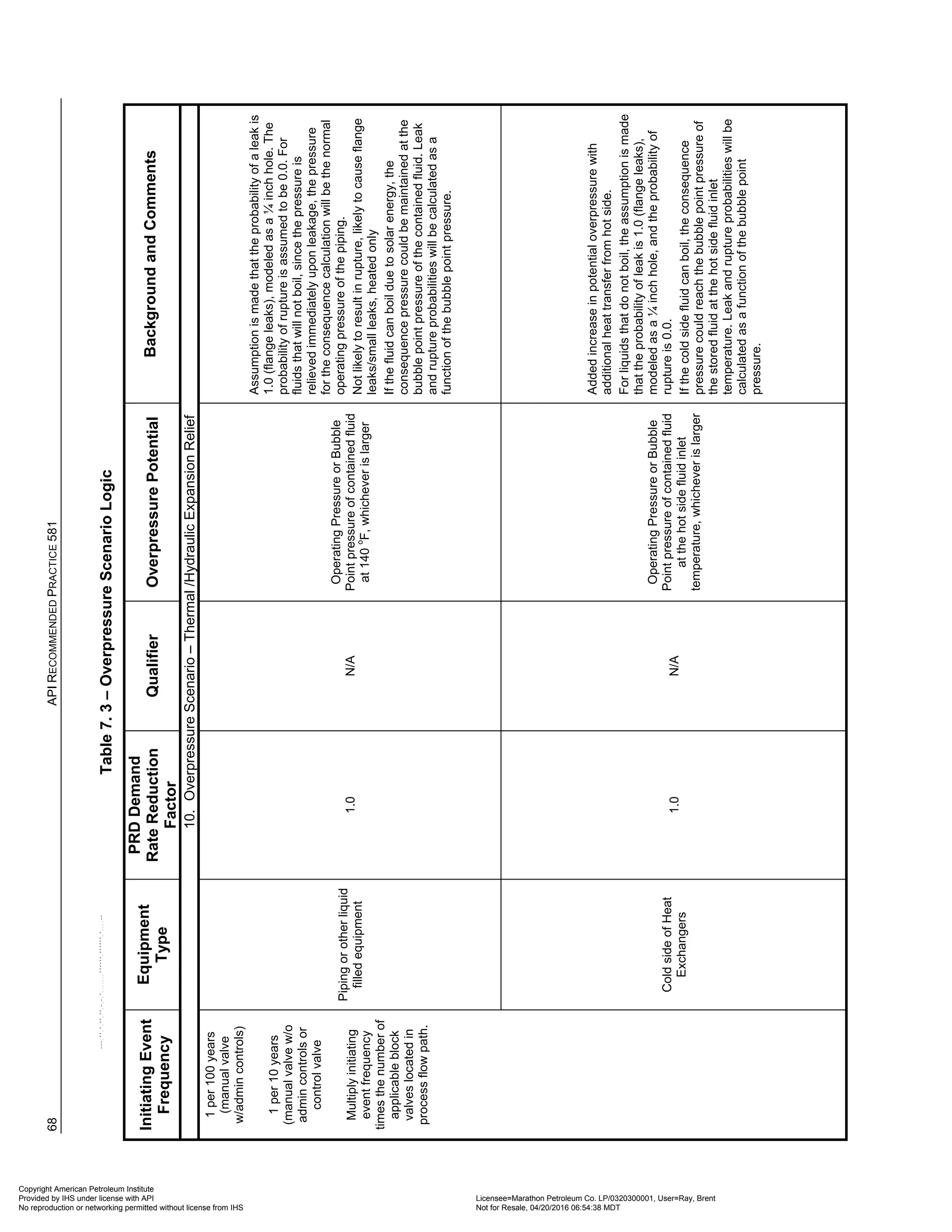
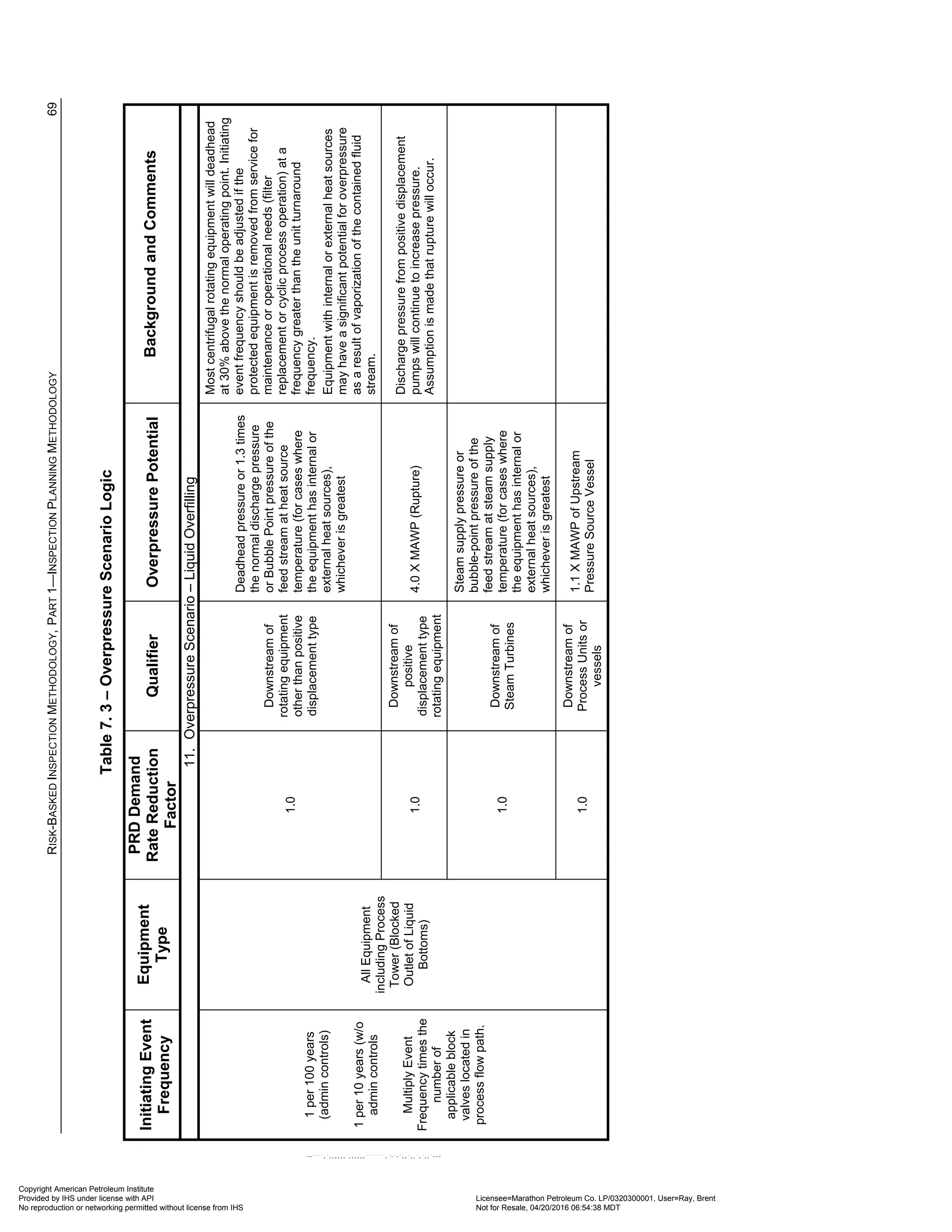
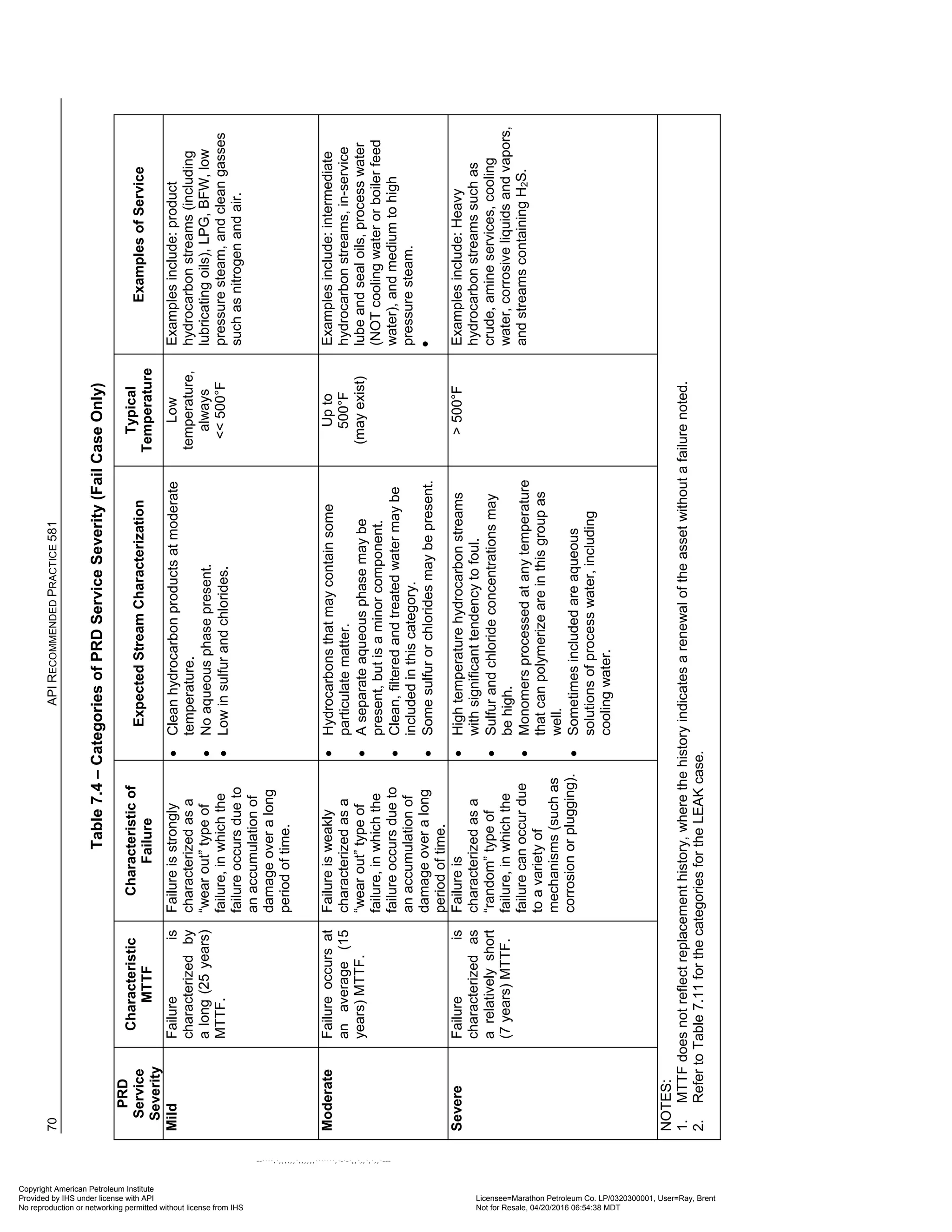
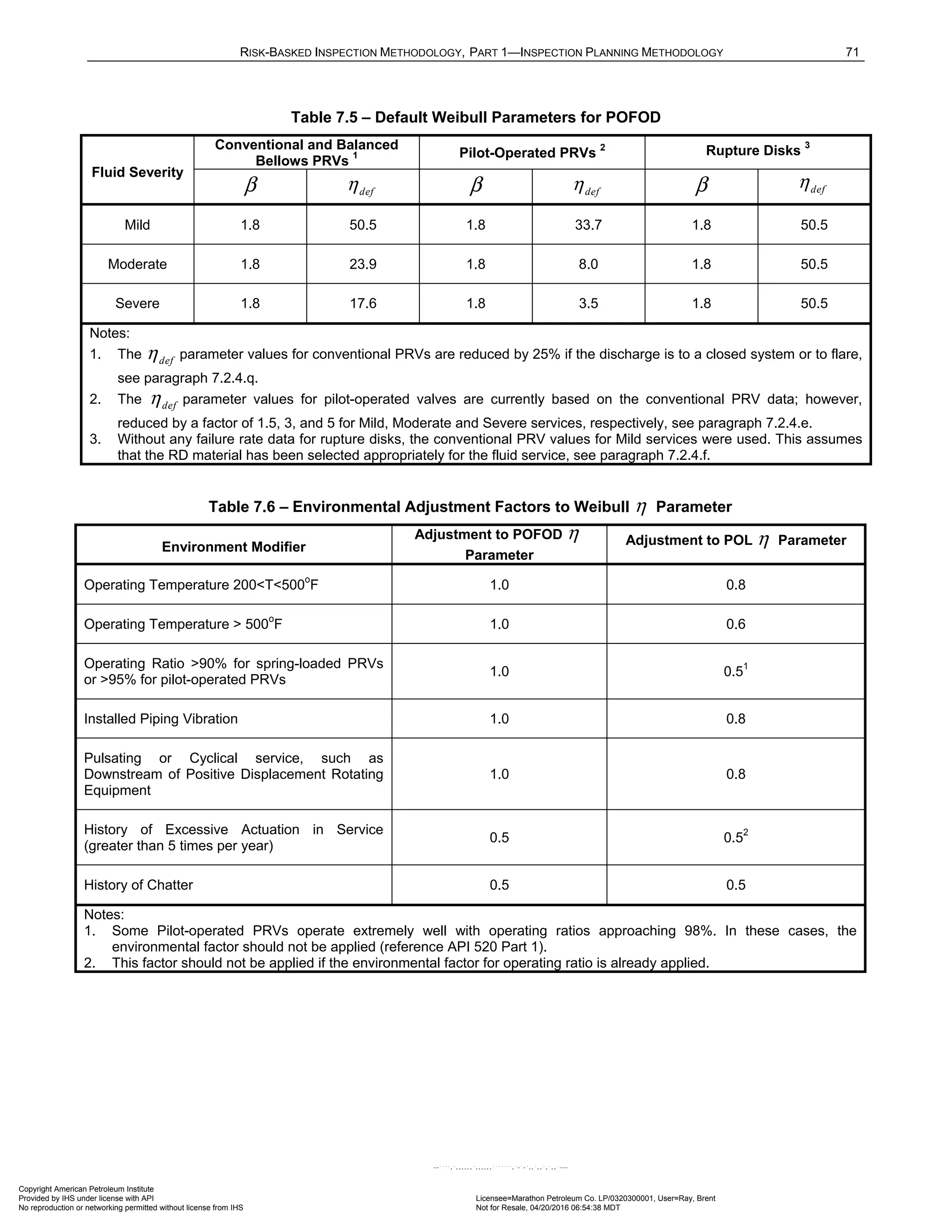
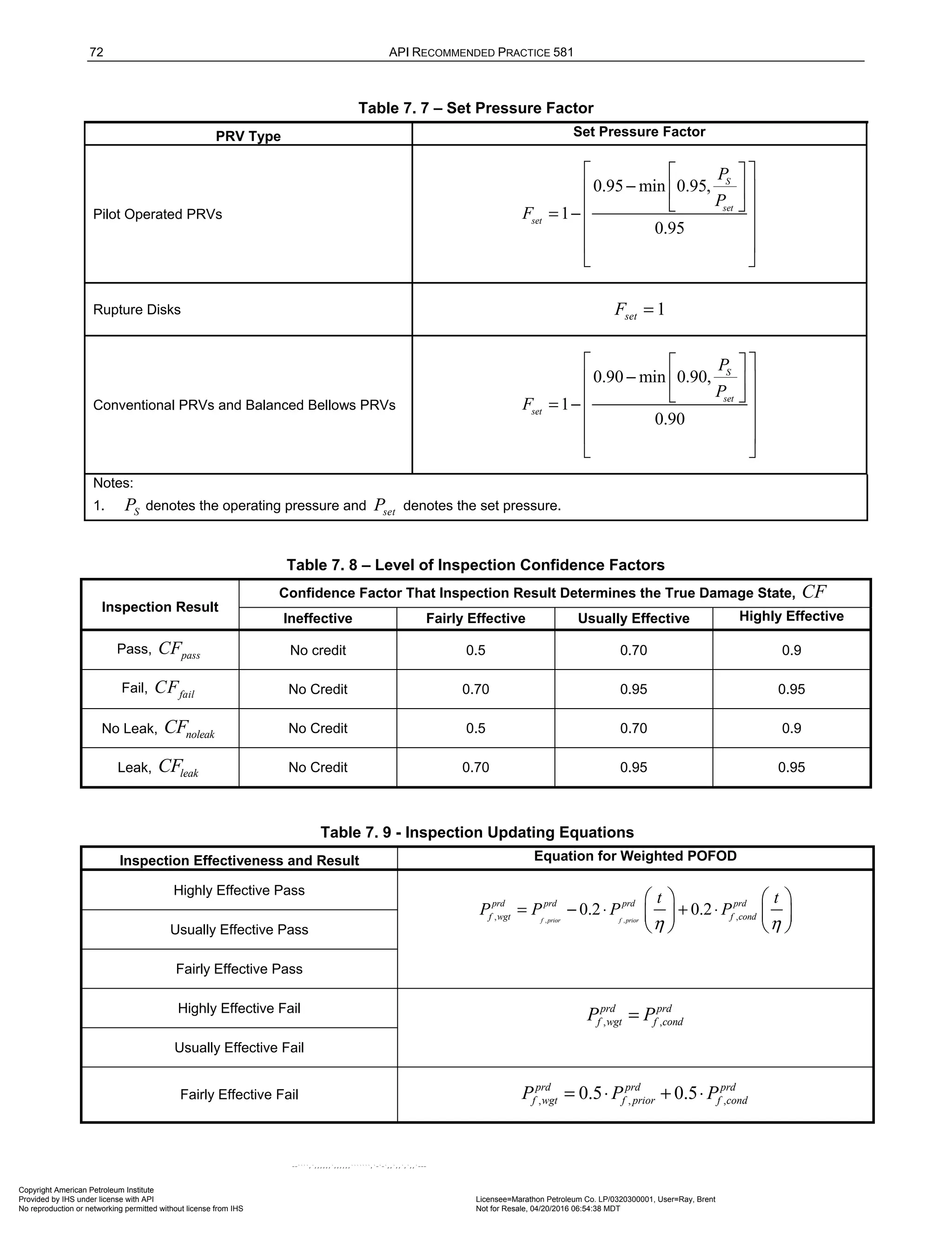
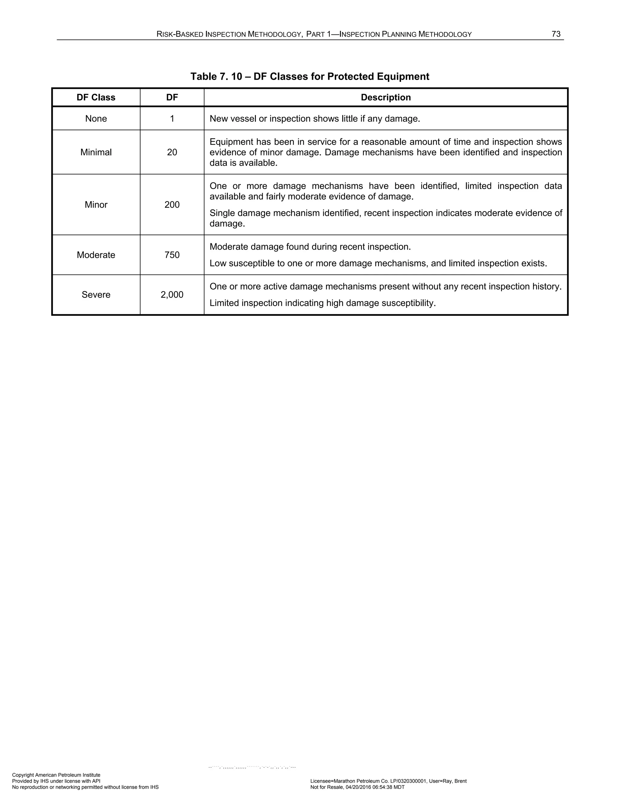
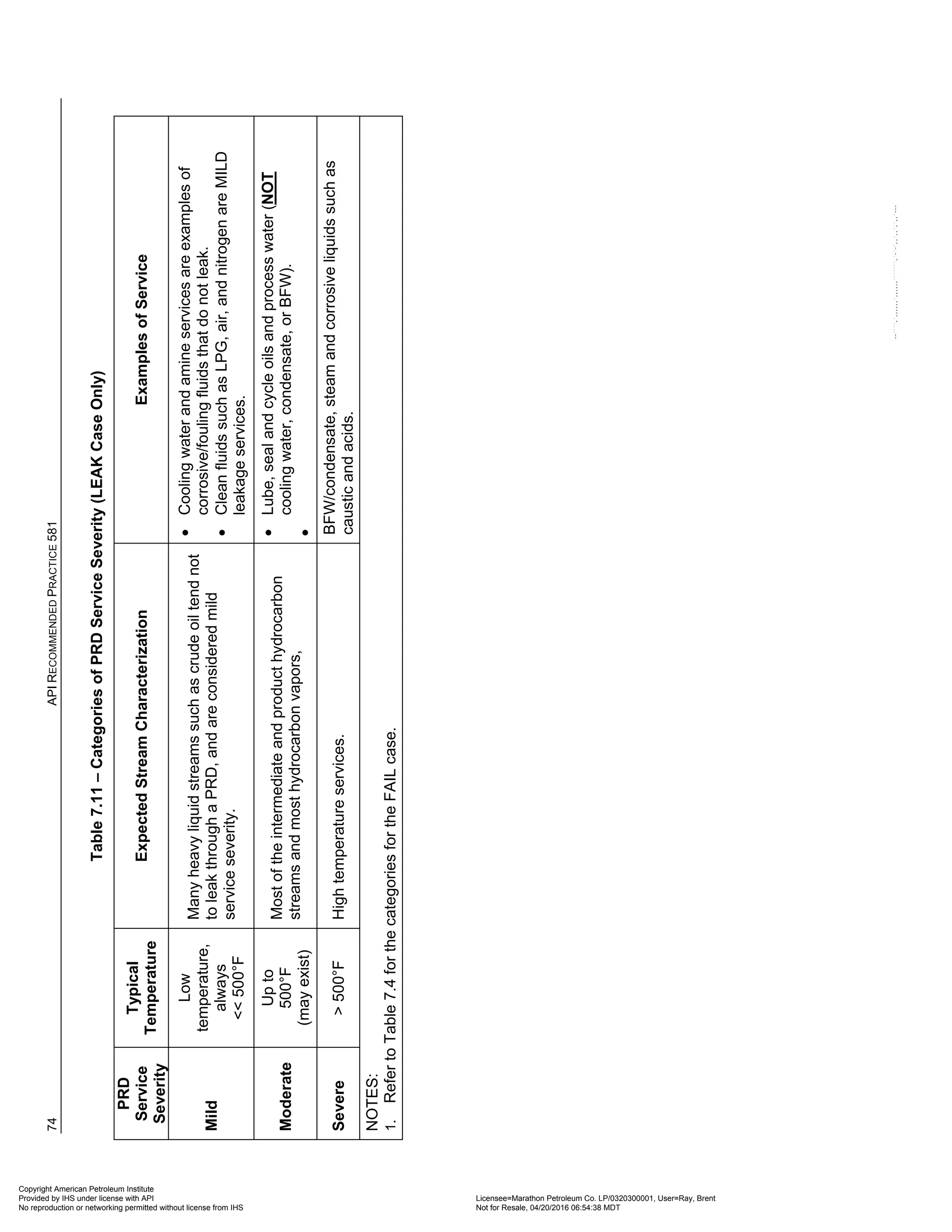
![RISK-BASKED INSPECTION METHODOLOGY, PART 1—INSPECTION PLANNING METHODOLOGY 75
Table 7.12 – Default Weibull Parameters for Probability of Leakage (POL)
Fluid
Severity
Conventional PRVs
1 Balanced Bellows
PRVs
1 Pilot-Operated PRVs
2
Rupture Disks
3
β def
η β def
η β def
η β def
η
Mild 1.6 17.5 1.6 16.0 1.6 17.5 1.6 17.5
Moderate 1.6 15.5 1.6 14.0 1.6 15.5 1.6 17.5
Severe 1.6 13.1 1.6 11.5 1.6 13.1 1.6 17.5
Notes:
1. The def
η parameter values are increased by 25% for Conventional and Balanced PRVs that have soft seats.
2. The def
η parameter values for pilot-operated valves are currently based on the conventional PRV data, since there is
currently no failure rate data to support otherwise.
3. Without any failure rate data for rupture disks, the conventional PRV values for Mild service were used.
Table 7.13 – Potential Consequences of Pressure Vessel Overpressure
Accumulation
(% over MAWP)
Significance[11] Potential Consequence
10%
ASME code allowable accumulation for
process upset cases (non-fire) protected by a
single relief device
No expected consequence at this accumulation
level.
16%
ASME code allowable accumulation for
process upset cases protected by multiple
relief devices
No expected consequence at this accumulation
level.
21%
ASME code allowable accumulation for
external fire relief cases regardless of the
number of relief devices
No expected consequence at this accumulation
level.
50%
ASME standard hydrostatic test pressure (may
be 30% on new designs)
Possible leaks in associated instrumentation,
etc. Medium consequence.
90%
Minimum yield strength (dependent on
materials of construction)
Catastrophic vessel rupture, remote possibility.
Significant leaks probable. Failure of damaged
vessel areas (corrosion, cracks, blisters, etc.
likely. High consequence.
300%
Ultimate tensile strength (dependent on
materials of construction)
Catastrophic vessel rupture predicted. Highest
consequence.
Copyright American Petroleum Institute
Provided by IHS under license with API Licensee=Marathon Petroleum Co. LP/0320300001, User=Ray, Brent
Not for Resale, 04/20/2016 06:54:38 MDT
No reproduction or networking permitted without license from IHS
--````,`,,,,,,`,,,,,,```````,`-`-`,,`,,`,`,,`---](https://image.slidesharecdn.com/api581-3rdedition-april2016-240227010601-3bf73ab5/75/Norma-API-581-3rd-Edition-April-2016-pdf-83-2048.jpg)
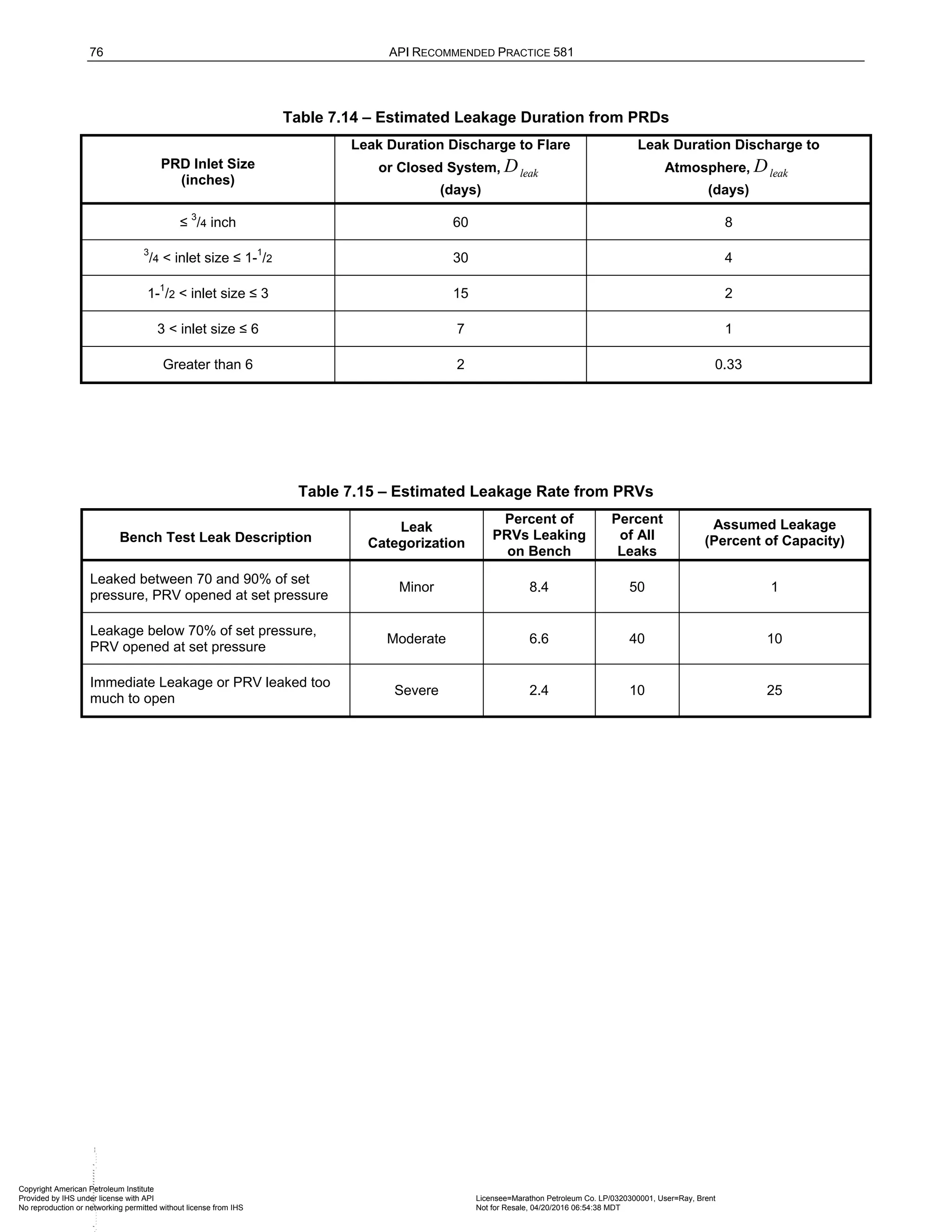
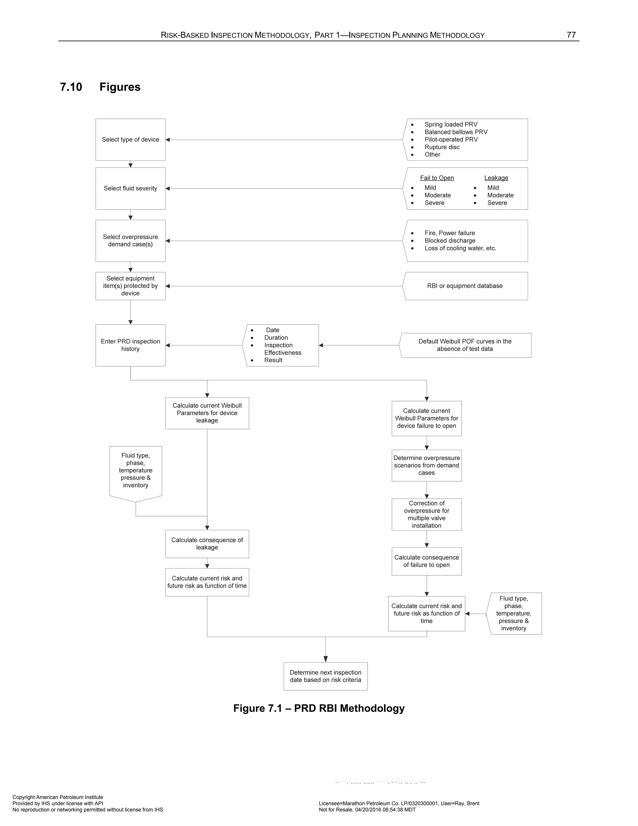
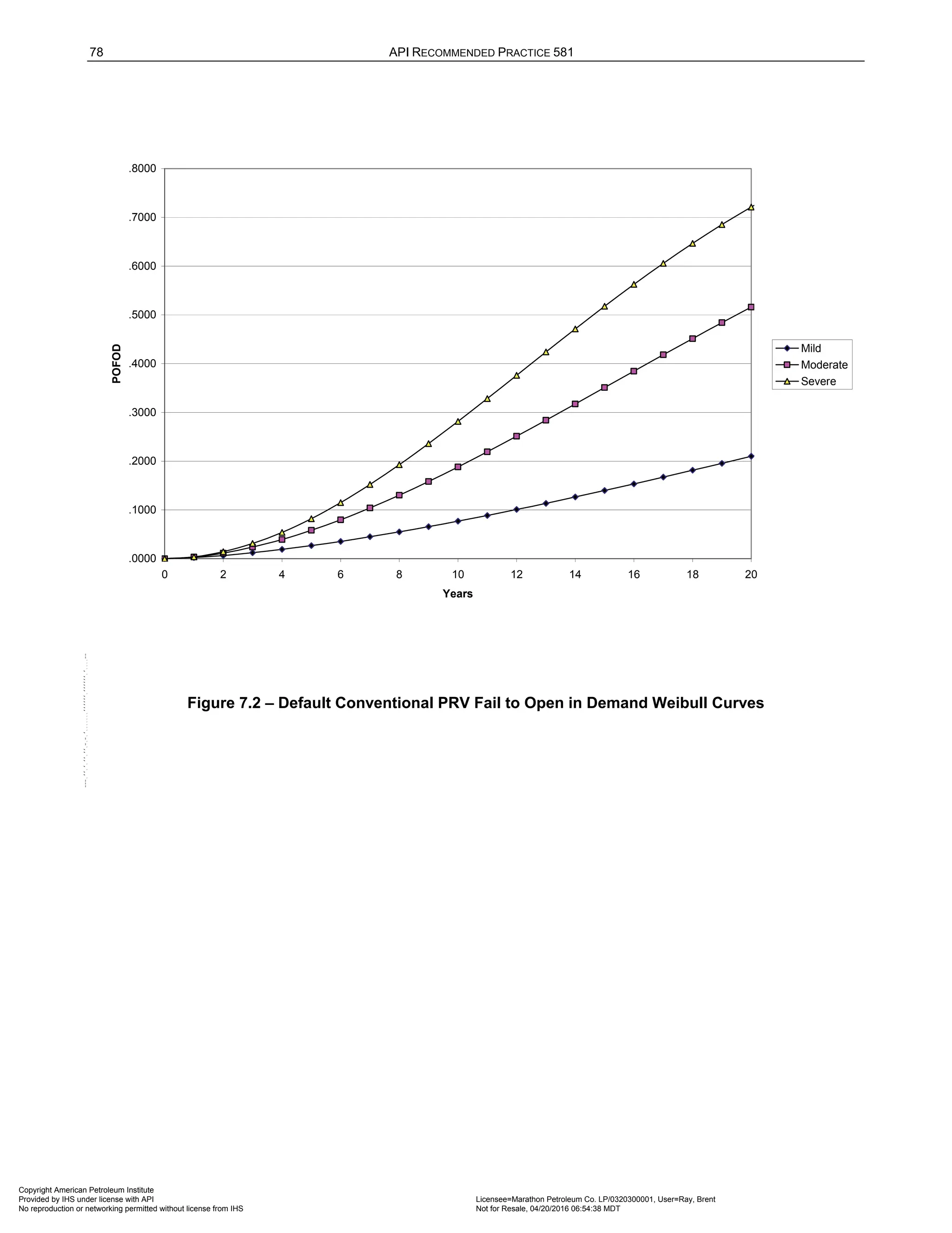
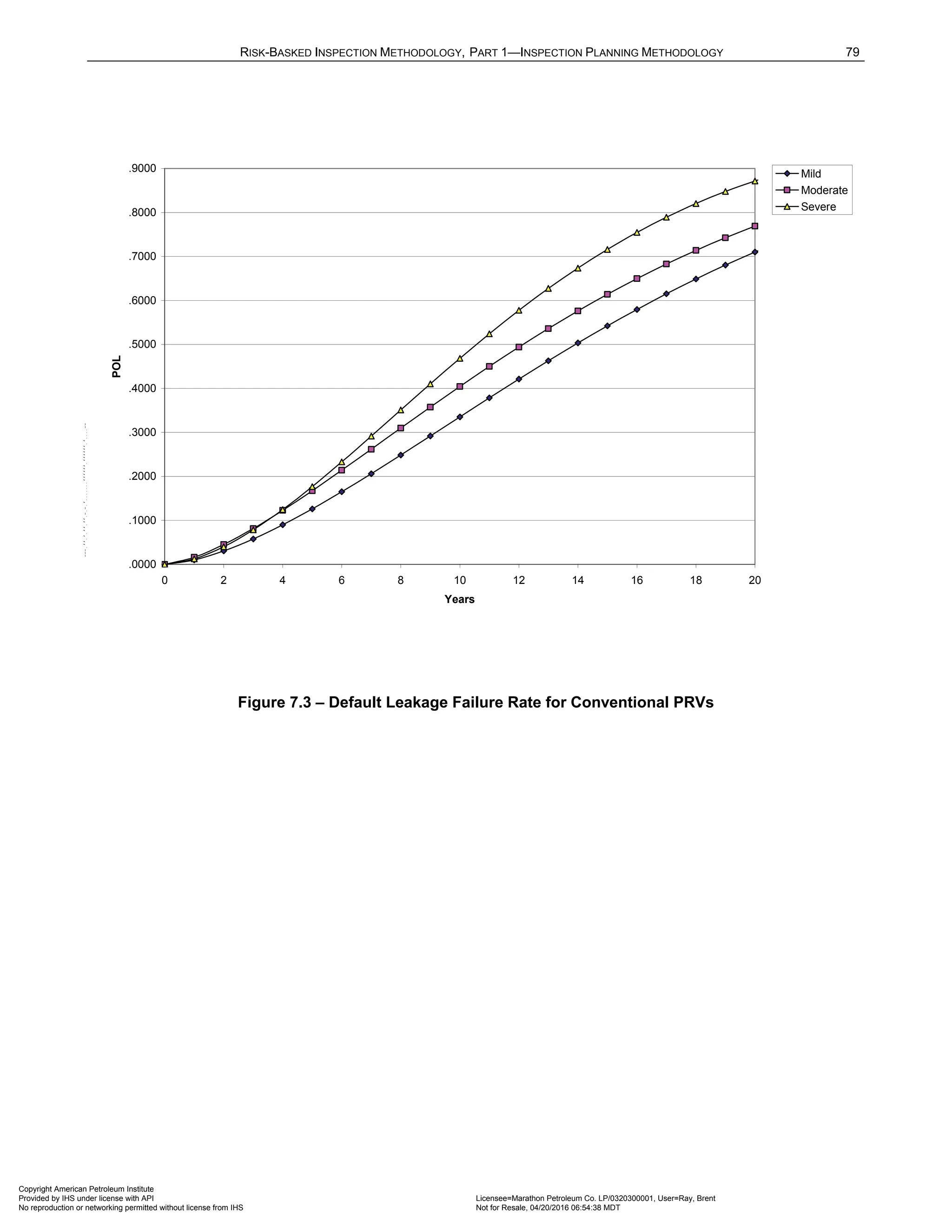
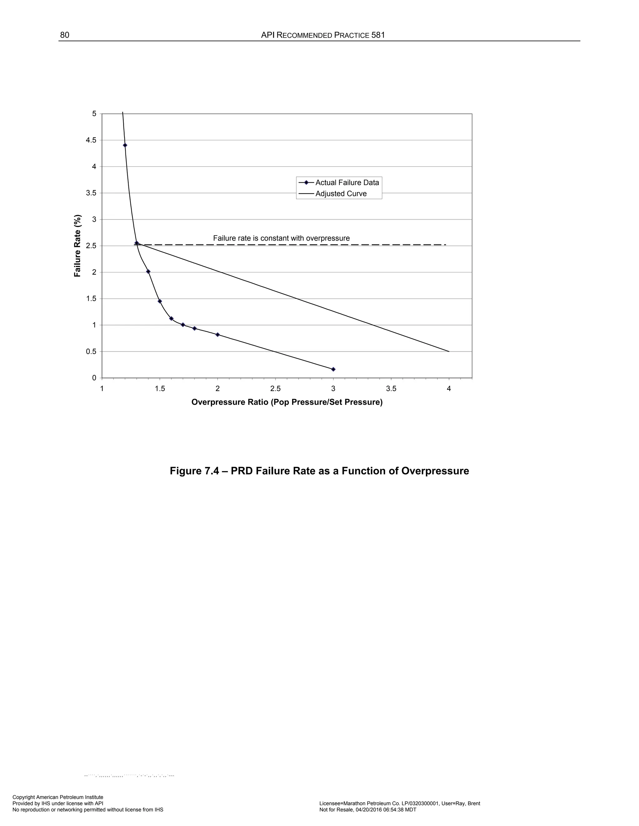
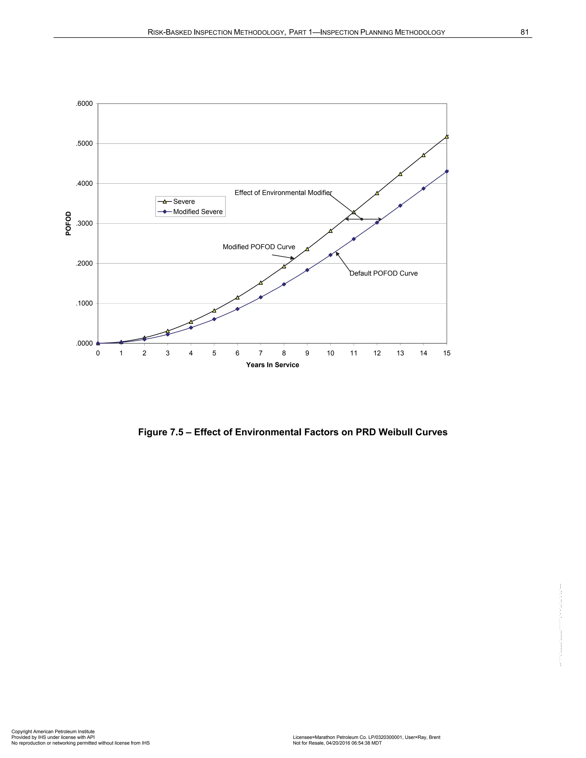
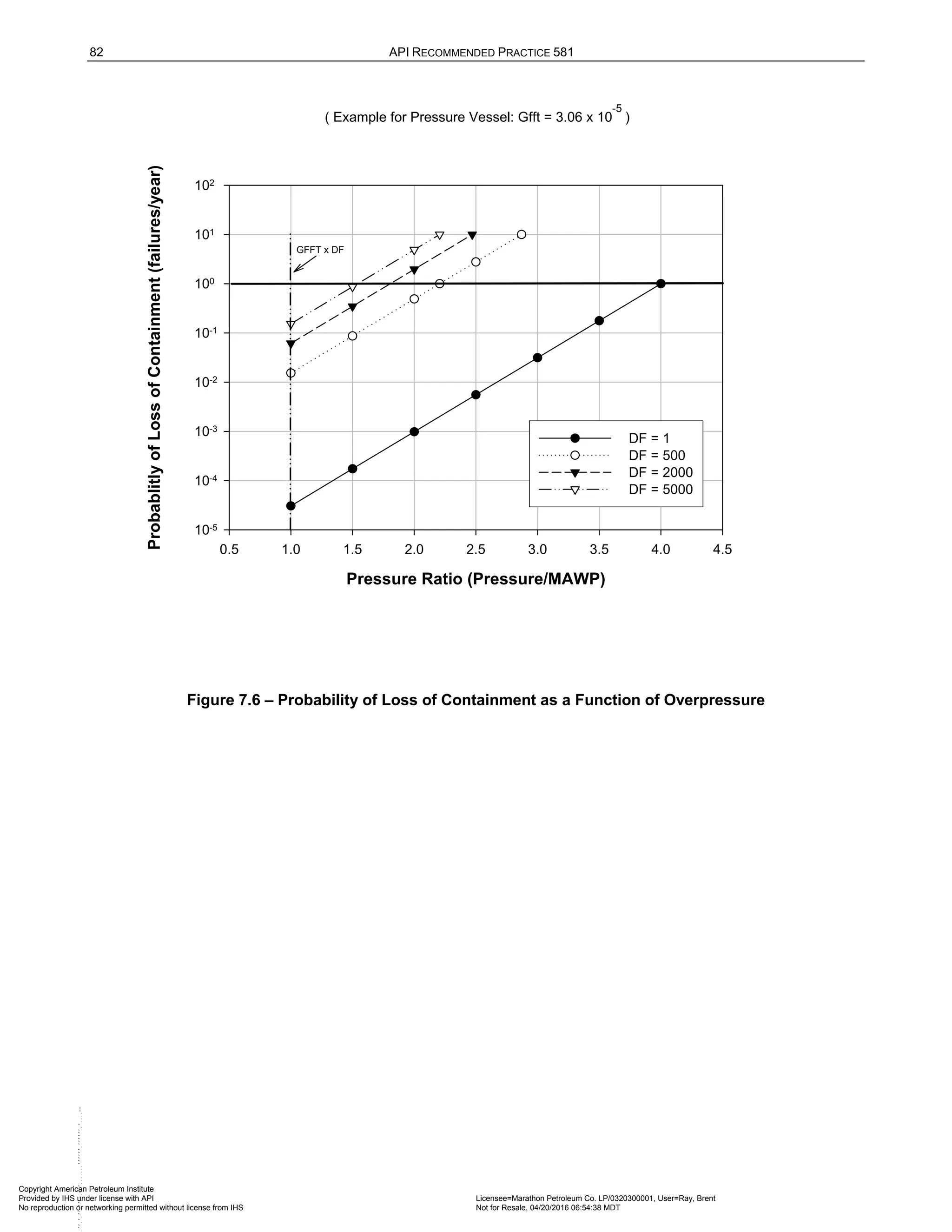
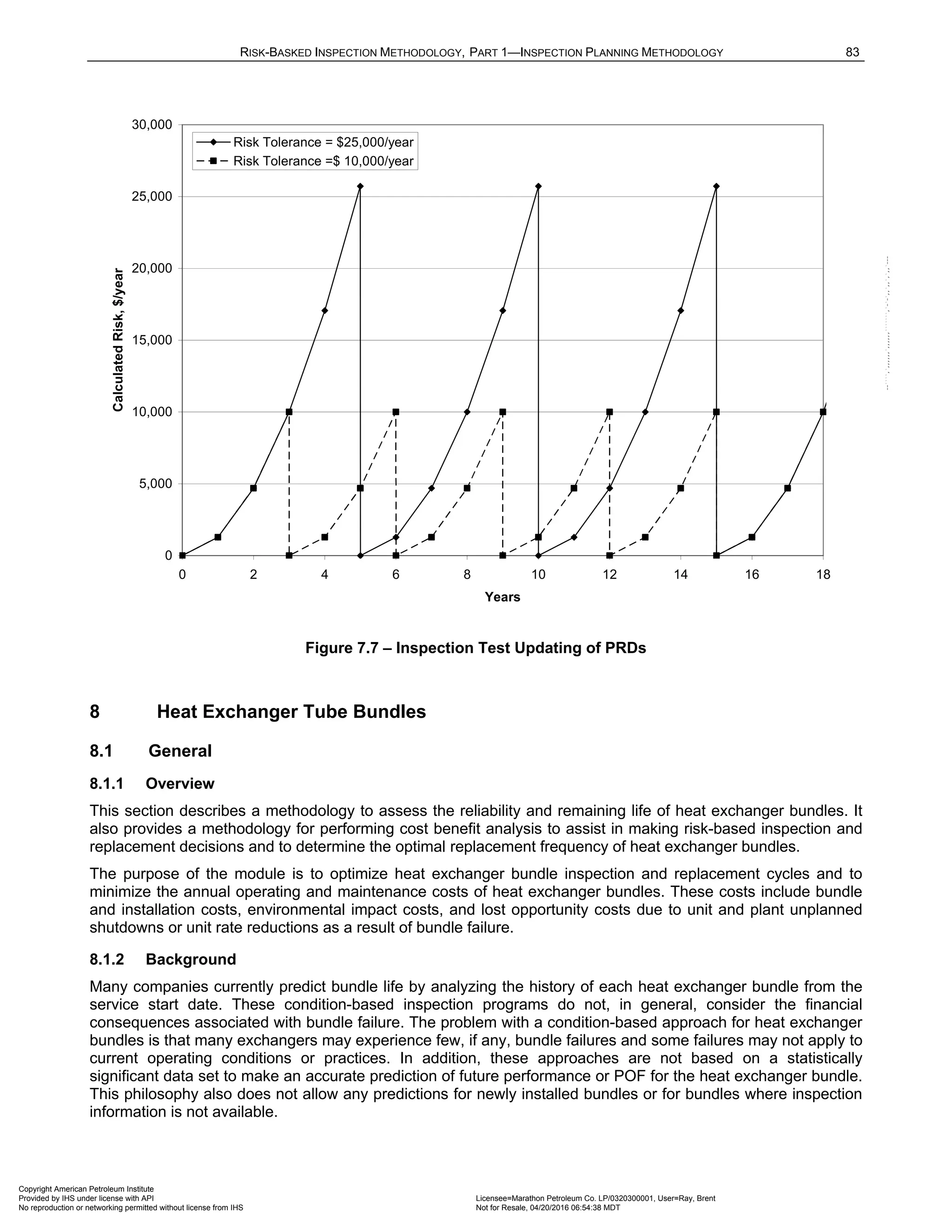
![84 API RECOMMENDED PRACTICE 581
8.1.3 Basis of Model
The application of risk principles to exchanger bundle inspection allows decisions to be made based on the
consequences of bundle failure, including costs associated with lost production and environmental impact costs
associated with leakage into utility systems and the replacement and maintenance costs associated with bundle
replacement.
To facilitate a more accurate prediction of future performance, the combined experience of other heat exchanger
bundles of similar design and in similar service may be combined and statistically analyzed. With this method, it
is critical that the owner-user maintains a heat exchanger bundle reliability library of failure data for exchanger
bundles. The exchanger bundle being evaluated is matched to a subset of similar bundles from the reliability
library and a Weibayes analysis is performed to estimate the future POF of the bundle. The results from the
analysis may be used to determine if the exchanger bundle will survive until the next scheduled maintenance
shutdown.
The advantage of using Weibayes analysis is that sound engineering decisions may be made with significantly
fewer failure data points as would be needed with other statistical distributions [11]. The Weibayes approach is
used as this method incorporates past experience of other similar bundles (Weibull library or seed database)
with the specific data available for the bundle being evaluated.
8.1.4 Required and Optional Data
The data listed in Table 8.1 shows the minimum data requirements for each heat exchanger bundle. In addition,
optional information can be supplied for the bundle being evaluated. The minimum and optional data are used
as matching criteria for the reliability library to filter the database down to a subset of bundles with similar
physical design and service. The more data that is used, the better the ability the user has to filter down to a
subset of bundles that is representative of the bundle being evaluated.
8.2 Methodology Overview
8.2.1 General
Calculations for the risk and inspection benefit of the heat exchanger bundles are performed following the flow
chart shown in Figure 8.1.
There are several steps involved in estimating the POF and the overall risks. The following steps describe the
methodology:
a) STEP 1 – Gather and input the bundle basic input data.
b) STEP 2 – Gather and input inspection historical data.
c) STEP 3 – Determine consequences of bundle failure,
tube
f
C .
d) STEP 4 – Determine the maximum acceptable POF based on the calculated
tube
f
C and the owner-user’s
risk target, tgt
Risk .
e) STEP 5 – Provide MTTF or Weibull parameters for the bundle failure rate curve, if known. If supplied, go
to STEP 12; otherwise proceed to STEP 6.
f) STEP 6 – Select a set of matching criteria and establish a cut-set of similar bundles from the reliability
library.
g) STEP 7 – Generate a Weibull plot of the cut-set data
h) STEP 8 – Assess the goodness of fit. Repeat cut-set selection (STEPs 6 and 7), if not acceptable.
i) STEP 9 – Determine Weibull parameters for the library cut-set data (raw data).
j) STEP 10 – Apply an uncertainty based on effectiveness of inspection to obtain the adjusted Weibull curve.
k) STEP 11 – If the inspection history provides thickness measurements or some other estimate of the current
condition and/or the remaining life for the bundle, adjust the Weibull curve to account for the known
condition of the bundle.
l) STEP 12 – Calculate the POF at the current date using the adjusted Weibull curve.
Copyright American Petroleum Institute
Provided by IHS under license with API Licensee=Marathon Petroleum Co. LP/0320300001, User=Ray, Brent
Not for Resale, 04/20/2016 06:54:38 MDT
No reproduction or networking permitted without license from IHS
--````,`,,,,,,`,,,,,,```````,`-`-`,,`,,`,`,,`---](https://image.slidesharecdn.com/api581-3rdedition-april2016-240227010601-3bf73ab5/75/Norma-API-581-3rd-Edition-April-2016-pdf-92-2048.jpg)
![RISK-BASKED INSPECTION METHODOLOGY, PART 1—INSPECTION PLANNING METHODOLOGY 85
m) STEP 13 – Calculate the risk at the plan date with and without inspection.
n) STEP 14 – Generate an inspection plan.
8.3 Probability of Failure
8.3.1 Definition of Bundle Failure
To be able to determine the bundle life (failure life) of bundles that are in the failure database and to predict the
point in time at which an existing bundle will reach its end of life, a definition of bundle failure must be
established. A failure is defined as a tube leak for the purposes of RBI.
When the controlling damage mechanism for the bundle is general corrosion, the current condition or remaining
life of a bundle can usually be quantified or expressed as a percent of the original wall thickness. Where
inspection records document average remaining wall thickness, this data may be used to determine when failure
occurred or to predict the point in the future where a failure is probable.
Other damage mechanisms, such as local corrosion, erosion, or vibration damage may not be easily predicted
based on measurements taken during an inspection. In these cases, prediction of the bundle failure may need
to be based on an estimation of remaining life of the bundle.
Typically, bundles are replaced or repaired prior to failure due to a deteriorated condition. In these situations,
one approach for estimating bundle failure is to assume that the bundle was replaced at 75% of the bundle life.
A 75% bundle life assumption is recommended and may be modified, if desired. The degraded condition
assumption allows consideration for remaining life of the bundle when replaced prior to actual tube failure. A
degraded condition is a bundle that would not be expected to make another operating cycle without expected
tube failures.
8.3.2 Probability of Failure Using Weibull Distribution
a) The POF for a heat exchanger bundle may be expressed using a two parameter Weibull distribution using
Equation (1.56) [12].
1 ( ) 1 exp
tube
f
t
P R t
β
η
= − = − −
(1.56)
In Equation (1.59),
tube
f
P is the POF as a function of time or the fraction of bundles that have failed at time
t. β is the Weibull shape factor that is unitless and η is the Weibull characteristic life in years, and t is
the independent variable time in years.
The time to reach a desired POF can be determined by rearranging Equation (1.56) as shown in
Equation (1.57).
( )
1
ln 1 tube
f
t P β
η
= ⋅ − −
(1.57)
b) The calculation of POF as a function of in-service duration may be performed using one of the methods
shown below:
1) Method 1 – Using matching criteria to filter on the reliability library, (see Section 8.3.2) – If a value of
the MTTF has not been specified, then the Weibull distribution is assumed and a Weibayes’ analysis is
performed on the matching bundles in the reliability library.
2) Method 2 – Owner-User Specified Weibull Parameters (see Section 8.3.4) – This involves
specification of the Weibull β and η parameters for the exchanger bundle being evaluated.
3) Method 3 – Owner-User Specified MTTF (see Section 8.3.4.2) – This involves the owner-user
providing the MTTF for the bundle being evaluated. The method will convert the MTTF to a Weibull
curve using a β value of 3.0. As an option, the Weibull β parameter in addition to the MTTF is
specified.
Copyright American Petroleum Institute
Provided by IHS under license with API Licensee=Marathon Petroleum Co. LP/0320300001, User=Ray, Brent
Not for Resale, 04/20/2016 06:54:38 MDT
No reproduction or networking permitted without license from IHS
--````,`,,,,,,`,,,,,,```````,`-`-`,,`,,`,`,,`---](https://image.slidesharecdn.com/api581-3rdedition-april2016-240227010601-3bf73ab5/75/Norma-API-581-3rd-Edition-April-2016-pdf-93-2048.jpg)
![86 API RECOMMENDED PRACTICE 581
4) Method 4 – Specific Bundle Inspection History (see Section 8.3.4.3) – Once enough inspection history
is accumulated, the statistics could be determined for the bundle.
8.3.3 Exchanger Bundle Reliability Library or Seed Database
a) General
A reliability database or Weibull library is extremely important to the evaluation of the risks associated with
bundle failure. Certain exchanger details are required to be gathered for each bundle entry in the reliability
database. Minimum basic data required for the database are indicated in Table 8.1. Optional data is also
shown in Table 8.1 that could be collected to provide additional matching/filtering capability for the reliability
library.
b) Weibayes Analysis
If the assumption is made that similarly designed bundles in similar service will have the same failure
mechanism, a Weibayes approach can be used. This approach assumes that the shape, or slope, of the
Weibull curve for the cut-set of similar bundles will be identical to the bundle that is being evaluated. The
Weibayes’ approach also allows an accurate statistical failure analysis to be performed without having a
large amount of failure data for the specific bundle being evaluated.
c) Developing Matching Criteria or Cut-Set
It is important to note that there are several different failure mechanisms that a heat exchanger bundle can
experience such as:
1) Corrosion
2) Pitting
3) Cracking
4) Erosion/corrosion
5) Vibration damage
6) Mechanical failure
7) Tube end thinning
The bundle reliability database is filtered using the parameters listed in Table 8.1. The goal is to filter the
database sufficiently enough to isolate the failure mechanism within the cut-set to one specific damage
mechanism, and to get the data to plot acceptably on a Weibull plot.
d) Goodness of Fit Test
If a Weibull plot is created from too broad of a cut-set on the failure reliability database, the data will not
properly plot on the Weibull plot. When this occurs, a likely reason is that multiple failure mechanisms are
being plotted and a more specific list of matching criteria is required to isolate the failures to one
mechanism.
A goodness of fit test should be used to determine whether or not the subset of data is correct. Once this is
accomplished, there is added confidence that the Weibull distribution of the cut-set is applicable to the
specific heat exchanger being evaluated.
Two approaches to the goodness of fit test for the data are the pve% and
2
r methods. The methodology
for determining these values are given in the New Weibull Handbook [14]. The closer the pve% is to 100,
the better the fit of the Weibull curve. In general, a pve% of greater than 20 is considered adequate for
small failure sample sizes (<20).
Copyright American Petroleum Institute
Provided by IHS under license with API Licensee=Marathon Petroleum Co. LP/0320300001, User=Ray, Brent
Not for Resale, 04/20/2016 06:54:38 MDT
No reproduction or networking permitted without license from IHS
--````,`,,,,,,`,,,,,,```````,`-`-`,,`,,`,`,,`---](https://image.slidesharecdn.com/api581-3rdedition-april2016-240227010601-3bf73ab5/75/Norma-API-581-3rd-Edition-April-2016-pdf-94-2048.jpg)
![RISK-BASKED INSPECTION METHODOLOGY, PART 1—INSPECTION PLANNING METHODOLOGY 87
e) Determination of Weibull Curve Parameters from Matching Data
After similar bundles have been matched from the database, the data has been plotted on a Weibull plot,
and a goodness of fit test has been applied, the Weibull parameters, β and η , are obtained. In
accordance with the Weibull Handbook [14], the standard method and best practice for estimating the
Weibull parameters, β and η for small and moderate sized data sets is median rank regression curve
fitting using the time-to-failure as the dependent variable (X onto Y).
Note that failure data as well as “no-failure” data (suspensions) are used in the plotting of the Weibull
curve.
f) Confidence Bounds
Most statisticians will use confidence bounds on data of this nature to account for the statistical distribution
in the data. A 90% lower bound confidence (LBC) interval is recommended using Fisher Matrix Bounds
[19]. The 90% LBC provides a 90% confidence that the data point will fall to the right of the line.
g) Example Calculation of POF using Weibayes’ with Failure Database
As an example of calculating a POF as a function of time in service for a hypothetical heat exchanger
bundle, a reliability database was searched to find bundles matching the following criteria:
1) Tubeside fluid category – Crude
2) Controlling damage mechanism – General corrosion
3) Tubeside operating temperature range between 350o
F and 500o
F
4) TEMA type AES
5) Exchanger type – liquid/liquid process exchanger
6) Sulfur content greater than 1%
Nine bundles in the database were retrieved. Five failures and four suspensions (bundles in-service without
failure reported) were found. The data is represented in Table 8.2.
The first three records shown in Table 8.2, noted by the exchanger tag number 191-X-25A, are data
accumulated from the inspection records for the specific bundle that is being evaluated. The remaining data
was obtained from similar bundles found in the reliability database.
The data supplied in Table 8.2 for the matching bundles has been plotted as a Weibull distribution on
Figure 8.2. The calculated Weibull parameters for this matching bundle set are:
2.568 slope parameter
β = (1.58)
20.45 characteristic life in years
η = (1.59)
The goodness of fit parameter, pve%, is shown on Figure 8.2 to be 99.9 which implies that the data
properly fits a Weibull distribution.
With the Weibull parameters defined, the POF as a function of time is determined for the example problem
using Equation (1.60).
2.568
1 exp
20.45
tube
f
t
P
= − −
(1.60)
8.3.4 POF Calculation Options
8.3.4.1 POF Using the Owner-User Supplied Weibull Parameters
As an option, the owner-user can provide the β and η parameters for the exchanger bundle and use
Equation (1.60) to determine the POF for the bundle as a function of time.
Copyright American Petroleum Institute
Provided by IHS under license with API Licensee=Marathon Petroleum Co. LP/0320300001, User=Ray, Brent
Not for Resale, 04/20/2016 06:54:38 MDT
No reproduction or networking permitted without license from IHS
--````,`,,,,,,`,,,,,,```````,`-`-`,,`,,`,`,,`---](https://image.slidesharecdn.com/api581-3rdedition-april2016-240227010601-3bf73ab5/75/Norma-API-581-3rd-Edition-April-2016-pdf-95-2048.jpg)
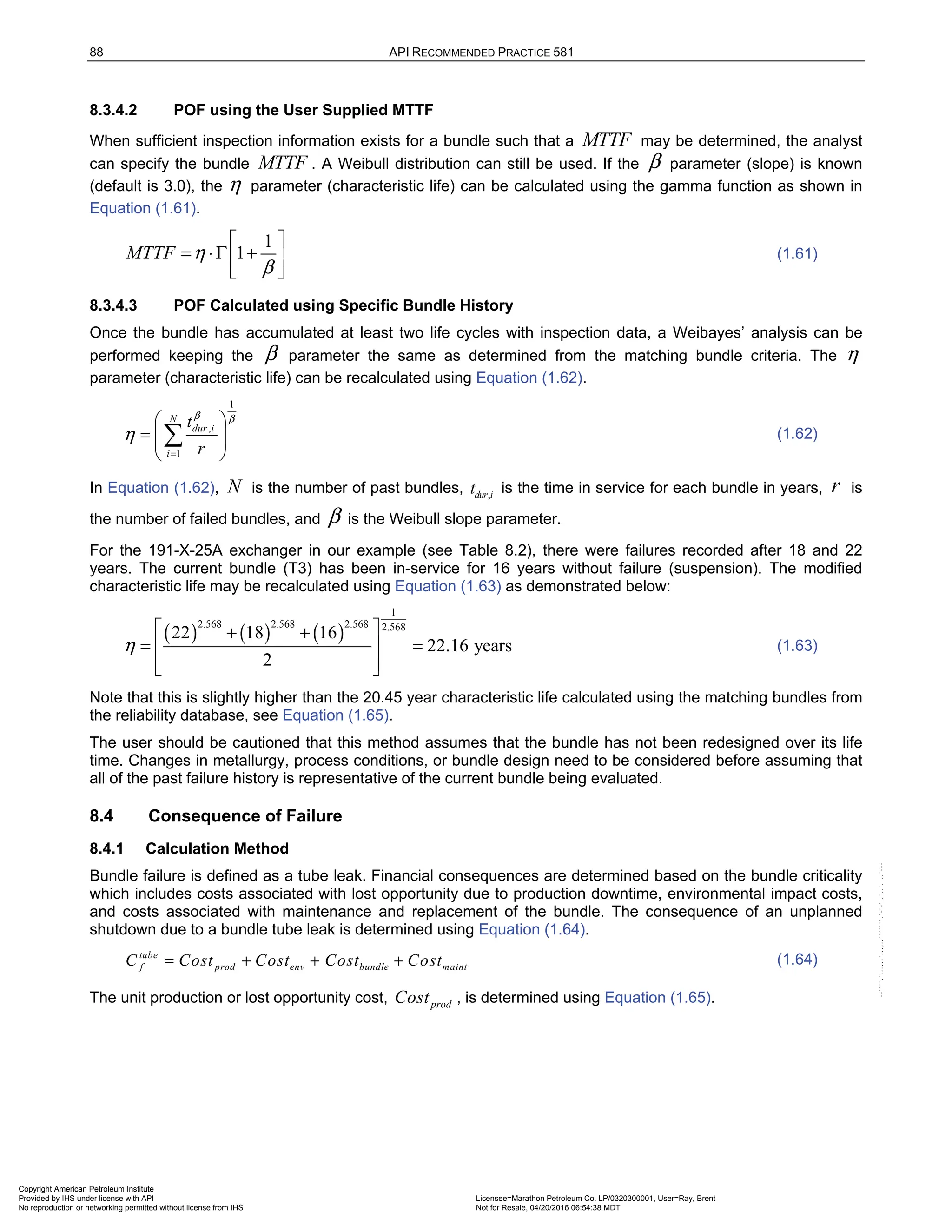
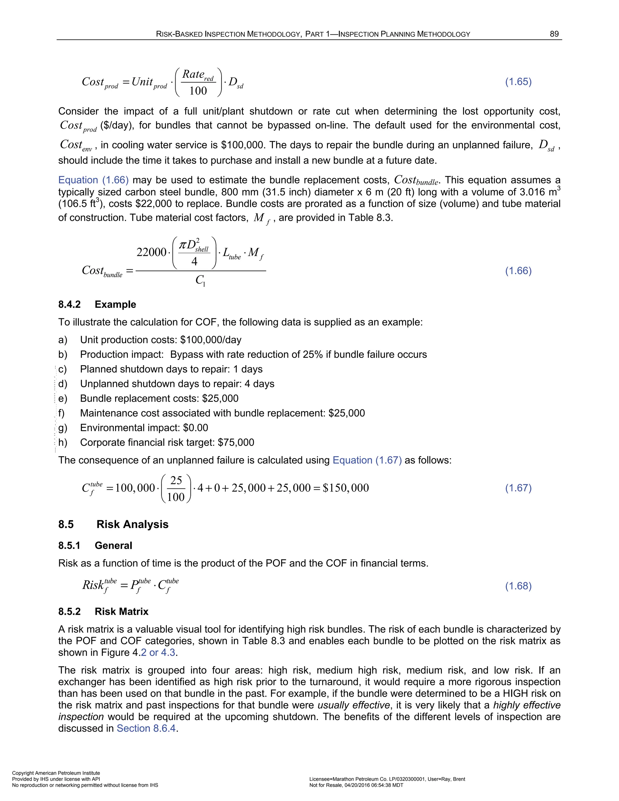
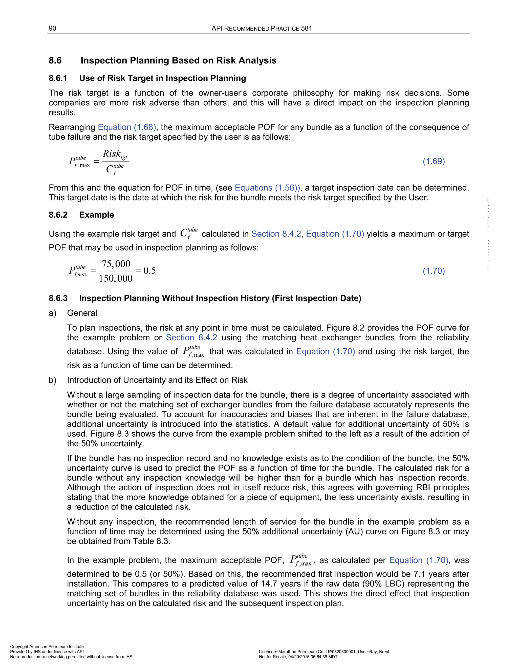

![RISK-BASKED INSPECTION METHODOLOGY, PART 1—INSPECTION PLANNING METHODOLOGY 93
( ) ( ) ( ) ( ) ( )
( ) ( ) ( ) ( )
1
2.568 2.568 2.568 2.568 2.568 2.568
2.568 2.568 2.568 2.568 2.568
18 22 16 10 12
1
27.2 years
6 13 14 25 8 (44.1)
mod
η
+ + + + +
= =
+ + + +
(1.77)
Plotting this as the failure point on the Weibull diagram results in a shift to the right as shown in
Figure 8.4. Note that the β parameter (Weibull slope parameter) was kept the same as the original curves
from data obtained from similar bundles. This is the basis of Weibaye’s analysis that assumes that similar
failure mechanisms will produce similar slope values.
The new POF curve in Figure 8.3 (second from left) shows the impact of the September 2003 inspection. In
the example problem, two adjustments to the right were made. The uncertainty was reduced from 50% (no
inspection) to 30% (“C” Inspection) as a result of the Elliot gauging/calipers measurements taken to
estimate the remaining wall thickness. Additionally, the base curve containing the raw data was shifted to
the right of the original raw data curve because the bundle was not in as poor condition as was expected
using the initial curve.
As a result, the recommended inspection interval at the maximum acceptable POF of 50% for the bundle
was increased from 7.1 years to 17.1 years or to February 2009. This calculation can be made using
Equation (1.78) as follows:
( ) [ ]
( )
1 1
2.568
ln 1 27.2 ln 1 0.5 17.1
tube
int mod f,max
t P years
β
η
= ⋅ − − = ⋅ − − =
(1.78)
8.6.5 Effects of Bundle Life Extension Efforts
In general, during an inspection, only minor repairs and cleaning operations are performed on exchanger
bundles. Bundles are not returned to an “as new” condition and therefore, the bundle POF is typically calculated
at a service duration (i.e., time in service) based on the bundle’s original installation date.
However, there are several life extension methods that may be made to a bundle during shutdowns that serve to
return the bundle back into service in an improved (not as-new) condition. In these situations, it would be too
conservative to calculate the future bundle POF based on the original service date, so an adjustment is made to
the start date for calculation purposes. Table 8.5 provides a list of life extension methods and the credit given as
represented by the life extension factor, LEF. An adjusted service duration, dur
tadj , is then calculated using the
LEF in accordance with Equation (1.79).
( )
1
dur dur
tadj LEF t
= − (1.79)
In Equation (1.80), the actual service duration, dur
t , is calculated as the time period (years) calculated from the
bundle original installation date to the inspection date when the life extension method was performed.
dur
t Inspect Date Install Date
= − (1.80)
The adjusted installation date from which all subsequent POF calculations are made is determined by
subtracting the adjusted service duration, dur
tadj (years), from the date when the life extension method was
performed as shown in Equation (1.81).
dur
Newinstall date= Inspect Date tadj
− (1.81)
8.6.6 Future Inspection Recommendation
Using the inspection adjusted failure rate curve as defined by the new Weibull parameters, the target date for
the next inspection can be determined. This will be the date at which the risk calculated using Equation (1.68)
exceeds the risk target, tgt
Risk , specified by the user. To maintain a risk level below the risk target, an
inspection will be required prior to that date. The question that needs to be answered is what level of inspection
is required to ensure that the risk target will not be exceeded during operation of the equipment.
Copyright American Petroleum Institute
Provided by IHS under license with API Licensee=Marathon Petroleum Co. LP/0320300001, User=Ray, Brent
Not for Resale, 04/20/2016 06:54:38 MDT
No reproduction or networking permitted without license from IHS
--````,`,,,,,,`,,,,,,```````,`-`-`,,`,,`,`,,`---](https://image.slidesharecdn.com/api581-3rdedition-april2016-240227010601-3bf73ab5/75/Norma-API-581-3rd-Edition-April-2016-pdf-101-2048.jpg)
![RISK-BASKED INSPECTION METHODOLOGY, PART 1—INSPECTION PLANNING METHODOLOGY 95
8.7.3 Decision for Type of Inspection
Once a decision has been made to inspect per Equation (1.83), an economic decision can be made as to the
appropriate level of inspection with similar techniques as described in Section 8.7.2 comparing the cost of the
various inspection techniques to the reduction in risk expected for the level of inspection.
8.7.4 Optimal Bundle Replacement Frequency
a) General
Maintenance optimization helps to strike a balance between cost and reliability. The cost per day of a "run
to failure" strategy shows low costs early in the life of the equipment and increasing costs as reliability
decreases. By overlaying the costs of an associated preventative maintenance to address the failure mode,
initial costs are high, but costs per unit time decrease as time progresses. This optimization occurs at a
point where the total cost function (sum of the two cost functions) is at a minimum. The time at which the
minimum occurs is the optimum time to perform maintenance [20].
For an exchanger bundle, the optimal replacement frequency can be determined by plotting the costs
associated with bundle failure (increases with increasing replacement frequency) to the replacement costs
associated with periodic planned shutdowns to replace the bundle (decreases with increasing replacement
frequency). The replacement frequency at which these two costs reach a minimum value, when averaged
over the expected bundle life, is the optimal replacement frequency.
The methodology in Shultz, 2001 [21] described below is recommended to determine the optimal frequency
for replacing bundles.
b) Increasing Risk Cost of Unplanned Outage
If the planned replacement time frequency is defined by the variable, tr , the risk cost associated with an
on-line failure (unplanned outage) to replace the bundle including business interruption and bundle
replacement costs is calculated using Equation (1.85).
( ) ( )
tube tube tube
f f f
Risk tr C P tr
= ⋅ (1.85)
where:
tube
f prod env bundle maint
C Cost Cost Cost Cost
= + + + (1.86)
The consequence of an unplanned outage due to a tube bundle failure,
tube
f
C , is identical to
Equation (1.64) and includes any environmental impact, env
Cost . The risk cost due to bundle failure
increases with time since the POF, ( )
tube
f
P tr , as a function of replacement frequency increases with time.
c) Decreasing Cost of Bundle Replacement
The bundle replacement costs as a function of planned replacement frequency, tr , is calculated using
Equation (1.87).
( ) ( )
, 1
tube tube
pbr f plan f
Cost tr C P tr
= ⋅ −
(1.87)
where:
, ,
100
tube red
f plan prod sd plan env bundle maint
Rate
C Unit D Cost Cost Cost
= ⋅ ⋅ + + +
(1.88)
Note that the cost of bundle replacement at a planned frequency includes downtime and business
interruption, however, the number of days for a planned outage, ,
sd plan
D , may be much less than if the
outage were unplanned due to a bundle failure. An unplanned outage would require some additional lead
time to get a replacement bundle on-site.
Copyright American Petroleum Institute
Provided by IHS under license with API Licensee=Marathon Petroleum Co. LP/0320300001, User=Ray, Brent
Not for Resale, 04/20/2016 06:54:38 MDT
No reproduction or networking permitted without license from IHS
--````,`,,,,,,`,,,,,,```````,`-`-`,,`,,`,`,,`---](https://image.slidesharecdn.com/api581-3rdedition-april2016-240227010601-3bf73ab5/75/Norma-API-581-3rd-Edition-April-2016-pdf-103-2048.jpg)
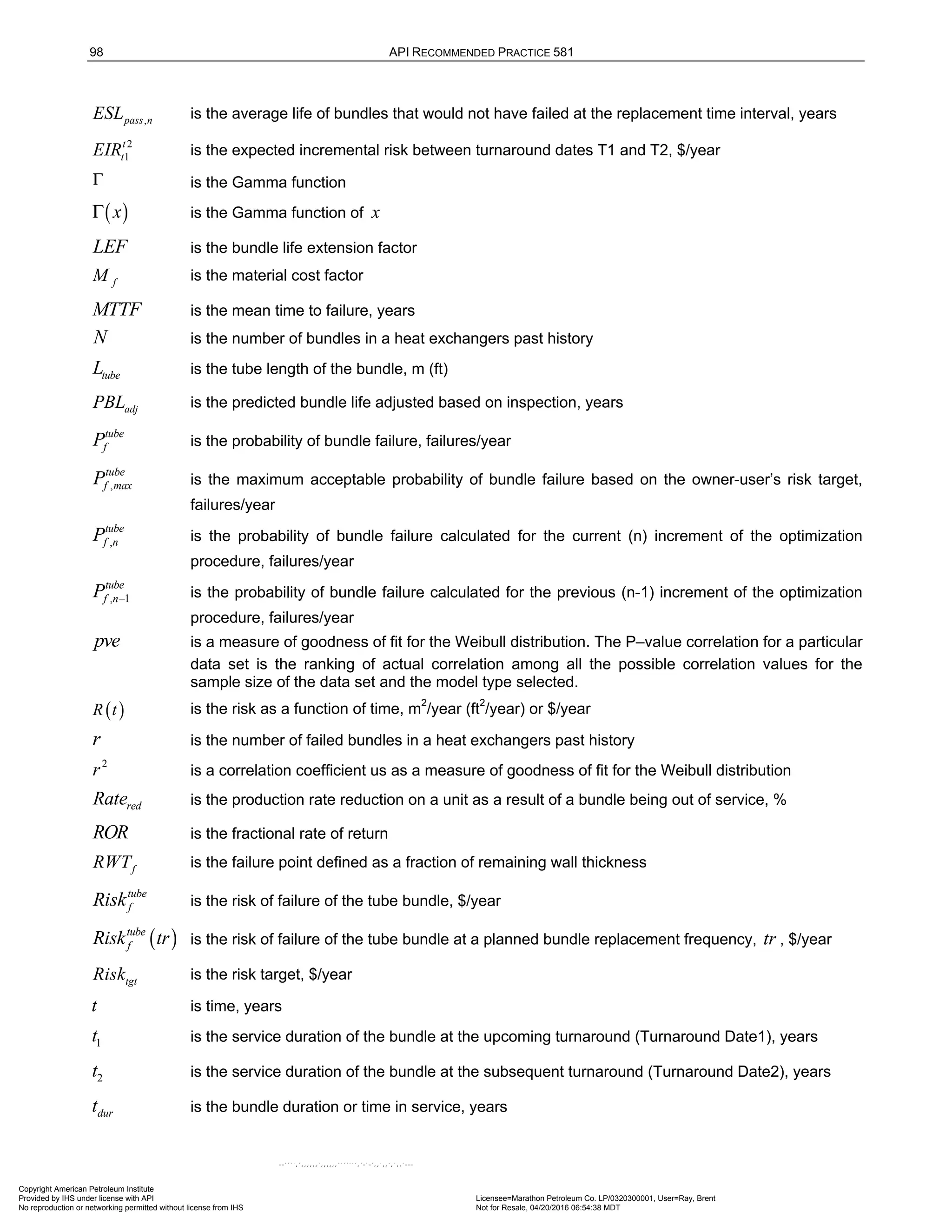
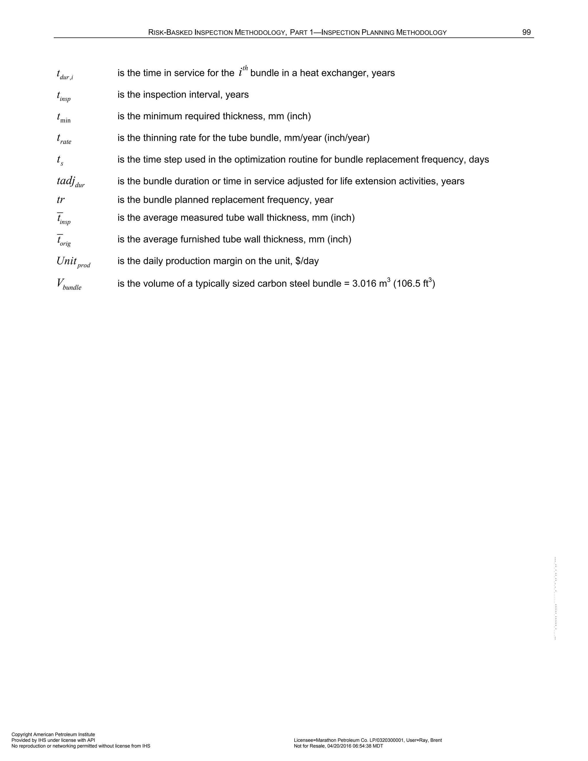
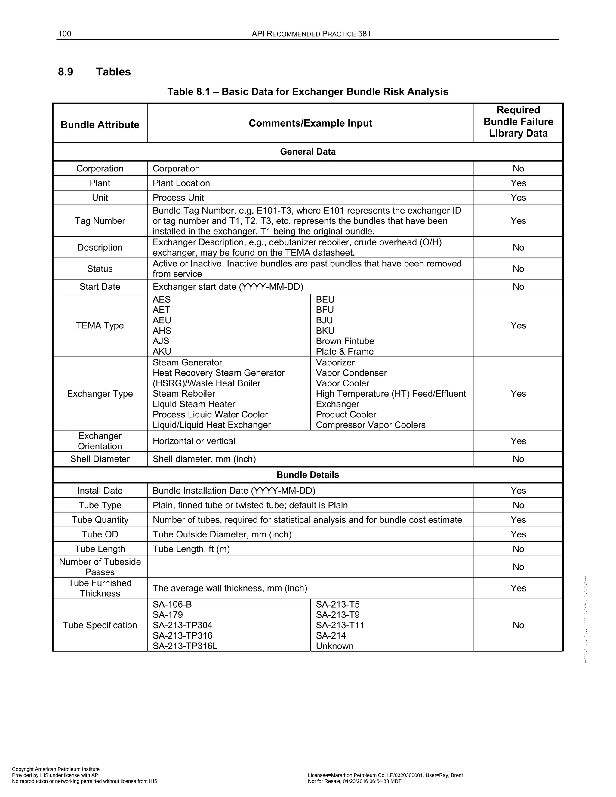
![RISK-BASKED INSPECTION METHODOLOGY, PART 1—INSPECTION PLANNING METHODOLOGY 101
Table 8.1 – Basic Data for Exchanger Bundle Risk Analysis
Bundle Attribute Comments/Example Input
Required
Bundle Failure
Library Data
Tube Material
Carbon Steel
C-1/2 Mo
1Cr
1.25Cr
2.25Cr
5Cr
9Cr
12Cr
304L/321/347
304/309/310
316L
317L
2205 Duplex SS
2304 Duplex SS
2507 Duplex SS
Ferralium 255
Zeron 100
Alloy 20Cb3
904L
AL6XN/254 SMO
430 SS
439 SS
444 SS
Sea-Cure/E-Brite
Admiralty Brass
Aluminum Brass
Red Brass
90/10 CuNi
70/30 CuNi
Monel 400
Alloy 800
Alloy 825
Alloy 600
Alloy 625
Alloy C276
Nickel 200
Titanium Gr. 2
Titanium Gr. 12
Titanium Gr. 16
Aluminum Alloy
Zirconium Alloy
Bimetallic
Ceramic
Plastic
Other
Yes
Tube Coating None, ID, OD, or both ID and OD No
U-Tube Post Weld
Heat Treatment
(PWHT)
Yes or No No
Impingement Plate Yes or No; may be found on the TEMA datasheet. No
Tube Layout
Triangular
Square
Rotated Square
Unknown
No
Tube Pitch Tube pitch, mm [inch] No
Baffle Type
Single Segmental
Double Segmental
Triple Segmental
Rod Baffle
Unknown
No
Baffle Cut Baffle Cut (%), may be found on the TEMA datasheet. No
Baffle Spacing Spacing between baffles, mm (inch), may be found on the TEMA datasheet. No
Tube Joint Design
Rolled Only
Seal Welded
Strength Welded
Unknown
Yes
Tubesheet Material
Specification
SA-105-II
SA-182-F5
SA-182-F9
SA-182-F11
SA-182-F316
SA-212-B-FBX
SA-240-TP304
SA-240-316L
SA-240-TP321
SA-266-II
SA-515-70
SA-516-70
Other
Unknown
No
Tubesheet Material
Carbon Steel
C-1/2 Mo
1Cr
1.25Cr
2.25Cr
5Cr
9Cr
12Cr
304L/321/347
304/309/310
316L
317L
2205 Duplex SS
Alloy 20Cb3
904L
AL6XN
430 SS
439 SS
Admiralty Brass
Aluminum Brass
Red Brass
90/10 CuNi
70/30 CuNi
Copper-other
Monel 400
Alloy 800
Alloy 825
Alloy 600
Alloy 625
Alloy C276
Nickel 200
Titanium Gr. 2
Aluminum Alloy
Zirconium Alloy
Ceramic
Plastic
Other
Unknown
No
Copyright American Petroleum Institute
Provided by IHS under license with API Licensee=Marathon Petroleum Co. LP/0320300001, User=Ray, Brent
Not for Resale, 04/20/2016 06:54:38 MDT
No reproduction or networking permitted without license from IHS
--````,`,,,,,,`,,,,,,```````,`-`-`,,`,,`,`,,`---](https://image.slidesharecdn.com/api581-3rdedition-april2016-240227010601-3bf73ab5/75/Norma-API-581-3rd-Edition-April-2016-pdf-109-2048.jpg)
![102 API RECOMMENDED PRACTICE 581
Table 8.1 – Basic Data for Exchanger Bundle Risk Analysis
Bundle Attribute Comments/Example Input
Required
Bundle Failure
Library Data
Tubesheet Cladding
Material
Carbon Steel
C-1/2 Mo
1Cr
1.25Cr
2.25Cr
5Cr
9Cr
12Cr
304L/321/347
304/309/310
316L
317L
2205 Duplex SS
2304 Duplex SS
2507 Duplex SS
Alloy 20Cb3
904L
AL6XN
430 SS
439 SS
Sea-Cure/E-Brite
Admiralty Brass
Aluminum Brass
Red Brass
90/10 CuNi
70/30 CuNi
Copper-other
Monel 400
Alloy 800
Alloy 825
Alloy 600
Alloy 625
Alloy C276
Nickel 200
Titanium Gr. 2
Titanium Gr. 12
Titanium Gr. 16
Aluminum Alloy
Zirconium Alloy
Non-metallic Coating
Plastic
Other
Unknown
No
Process/Operating Conditions (Tubeside and Shellside)
Process Unit
Amine Regeneration
Amine Treating
Aromatics Recovery
Continous Catalytic Reforming (CCR)
Catalytic Reforming (Fixed)
Caustic Treating (Merox)
Crude Distillation Unit
Cumene
Delayed Coker
Distillate Fractionator
Fluid Coker
Dimersol
Ether Plant (Methyl Tertiary Btuyl
Ether[MTBE]/ Tertiary Amyl Methyl
Ether [TAME])
Fluid Catalytic Cracking
Sat Gas Plant
Unsat Gas Plant
Gas Separation
HF Alkylation
Hydrotreater/Hydrocracker
Hydrocracker (2nd Stage)
Hydrogen Reforming
Isomerization
LPG Refrigeration
Lube Plant
Polymerization
Partial Oxidation
Selective Hydrogenation
Sour Water Stripper
Sulfolane
Sulfur Recovery Unit
Sulfuric Acid Alkylation
Sulfuric Acid Plant
Tail Gas Treater
Thermal Cracking
Vacuum Unit
Cooling Tower Water
Cooling Water – other
Yes
Fluid Name Generic Name, e.g., crude, effluent, heavy gas oil (HGO), etc. No
Copyright American Petroleum Institute
Provided by IHS under license with API Licensee=Marathon Petroleum Co. LP/0320300001, User=Ray, Brent
Not for Resale, 04/20/2016 06:54:38 MDT
No reproduction or networking permitted without license from IHS
--````,`,,,,,,`,,,,,,```````,`-`-`,,`,,`,`,,`---](https://image.slidesharecdn.com/api581-3rdedition-april2016-240227010601-3bf73ab5/75/Norma-API-581-3rd-Edition-April-2016-pdf-110-2048.jpg)
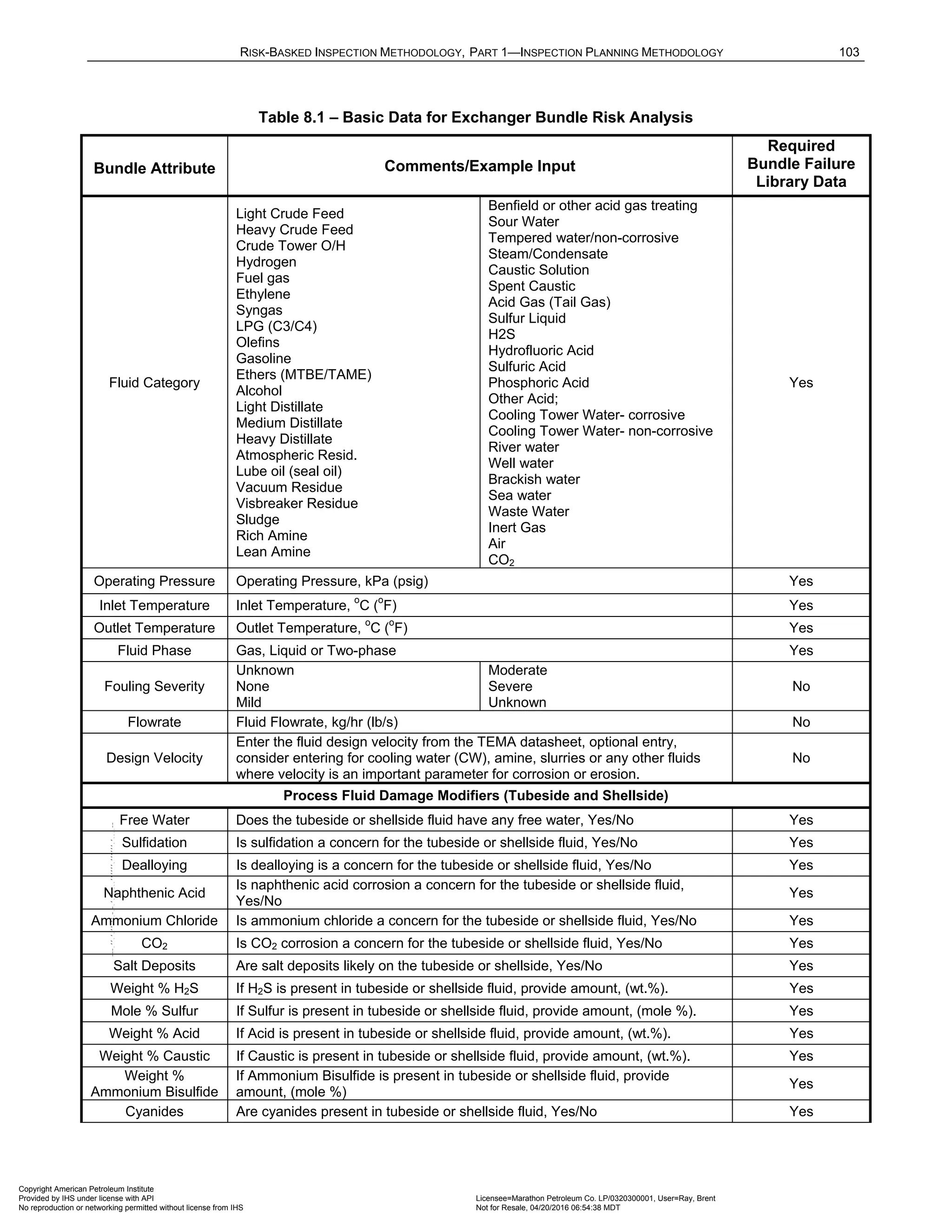
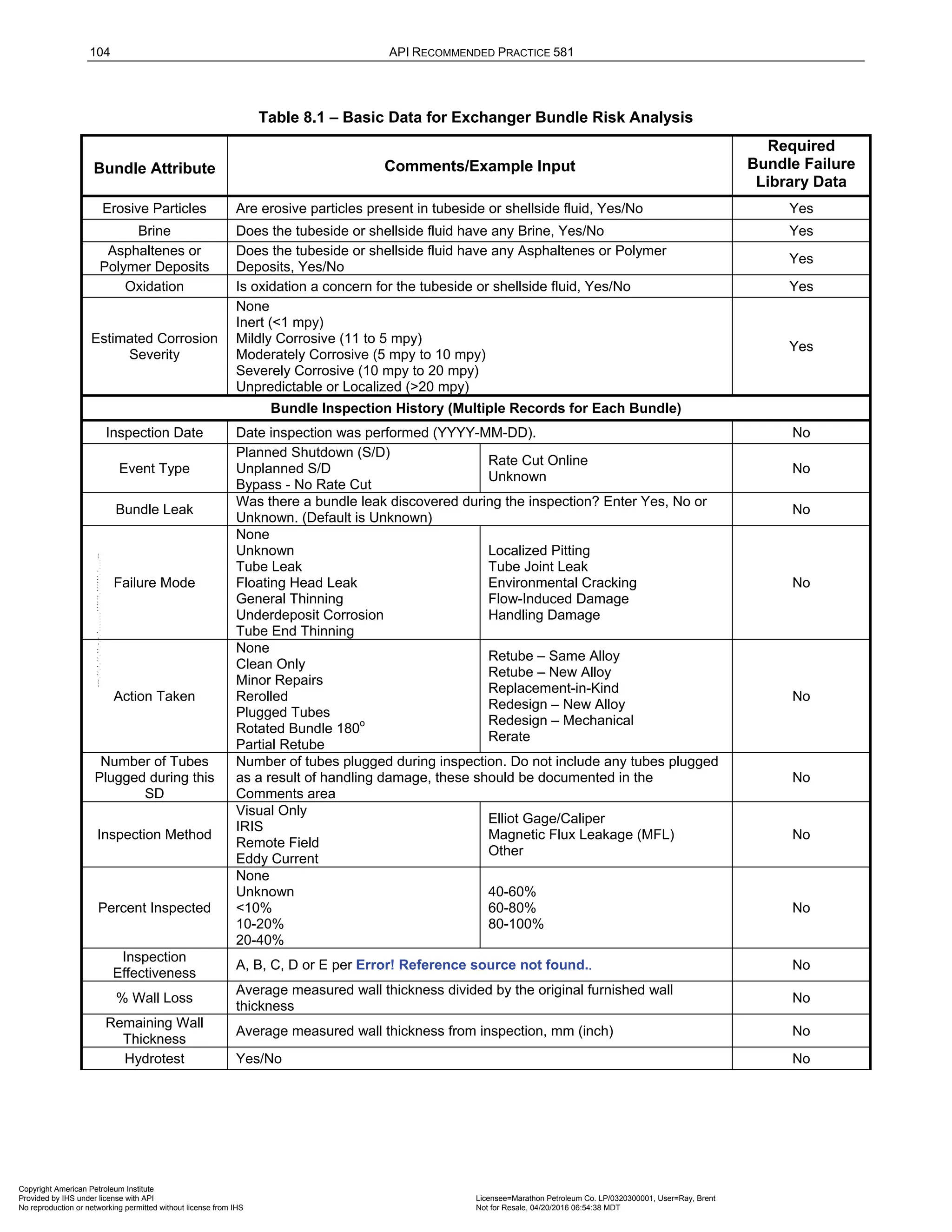
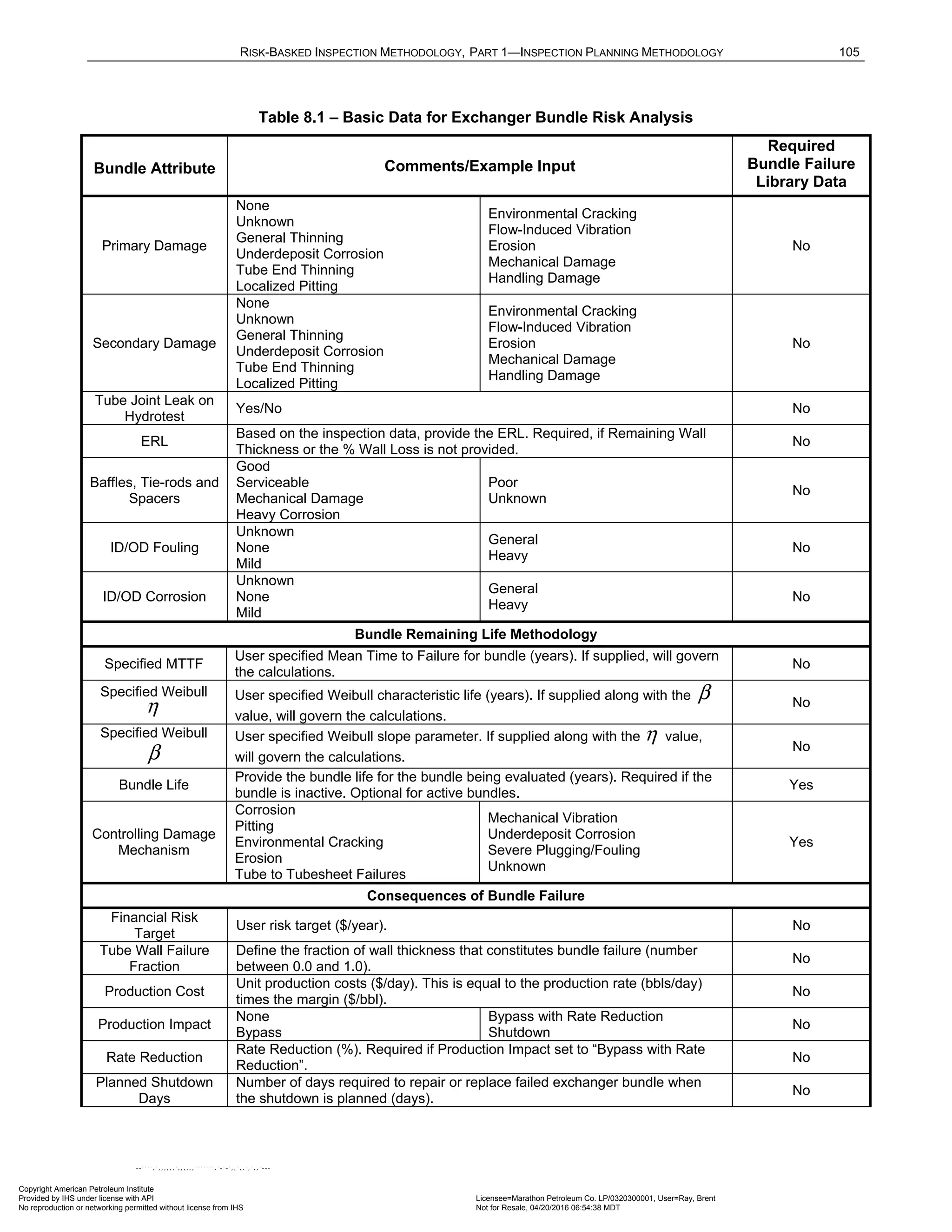
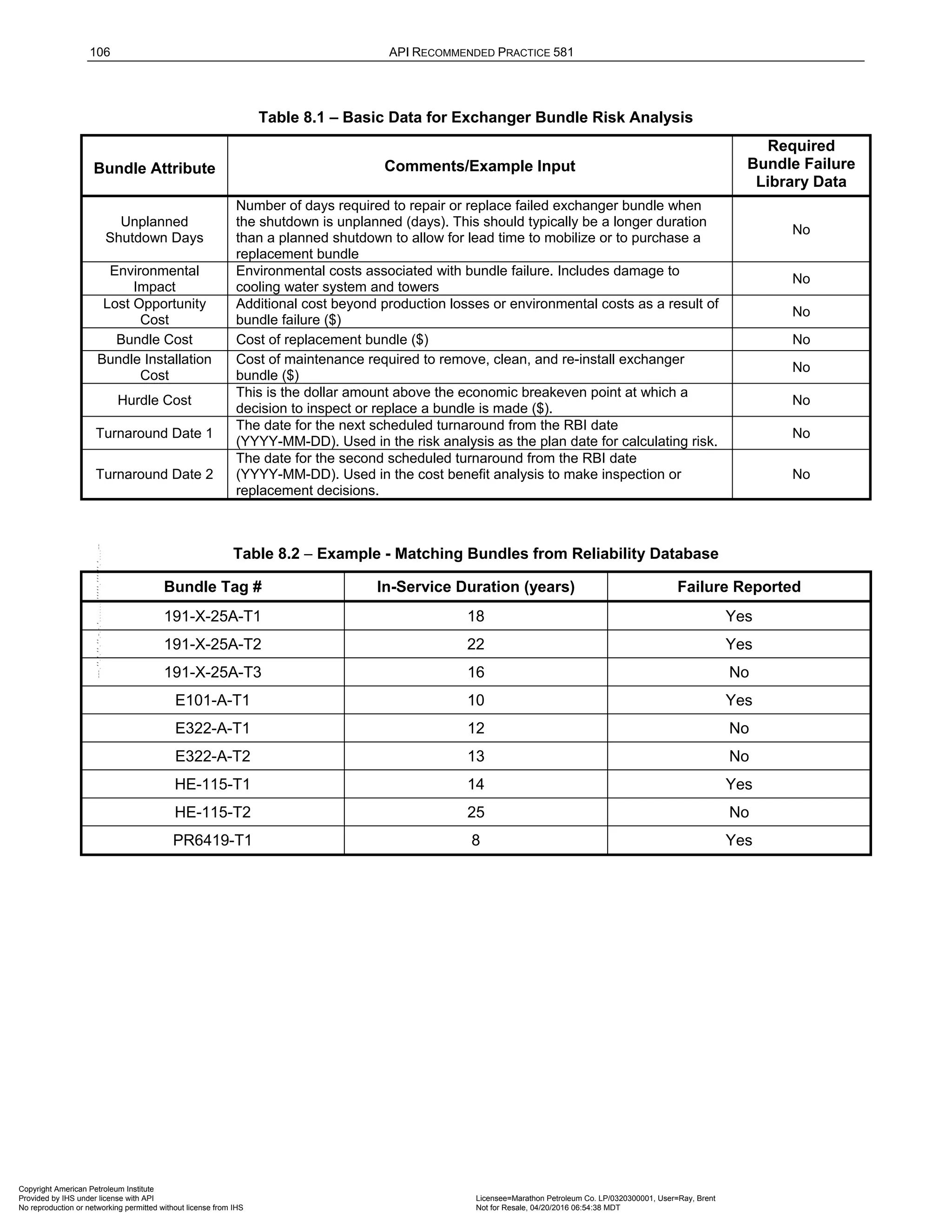
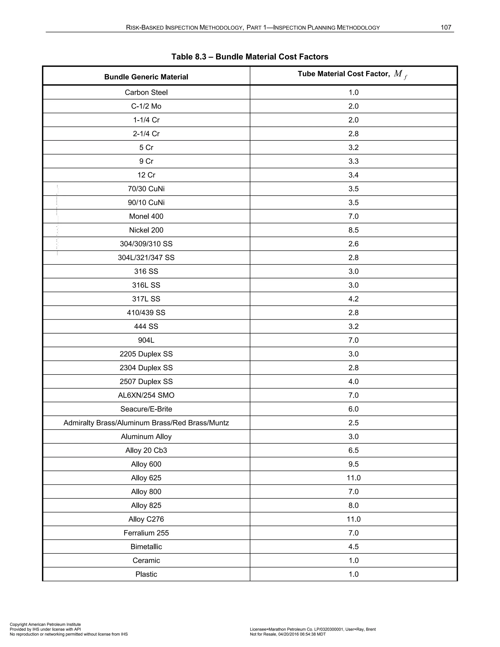
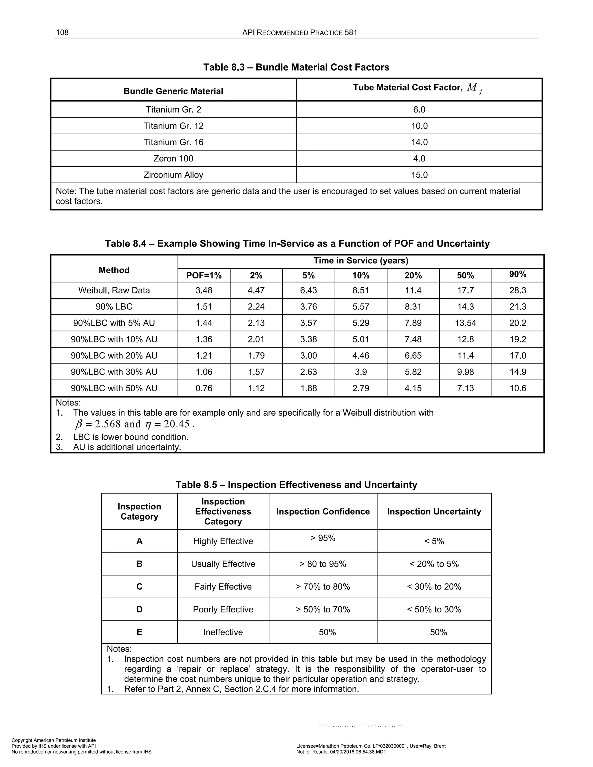
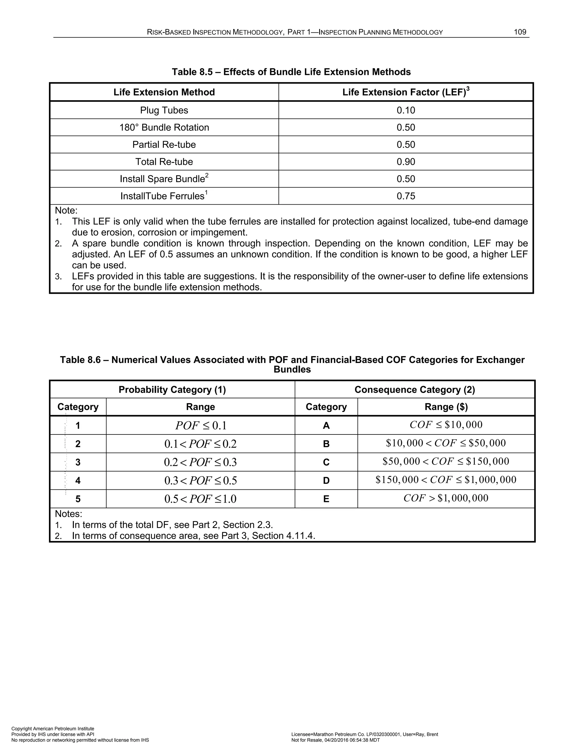
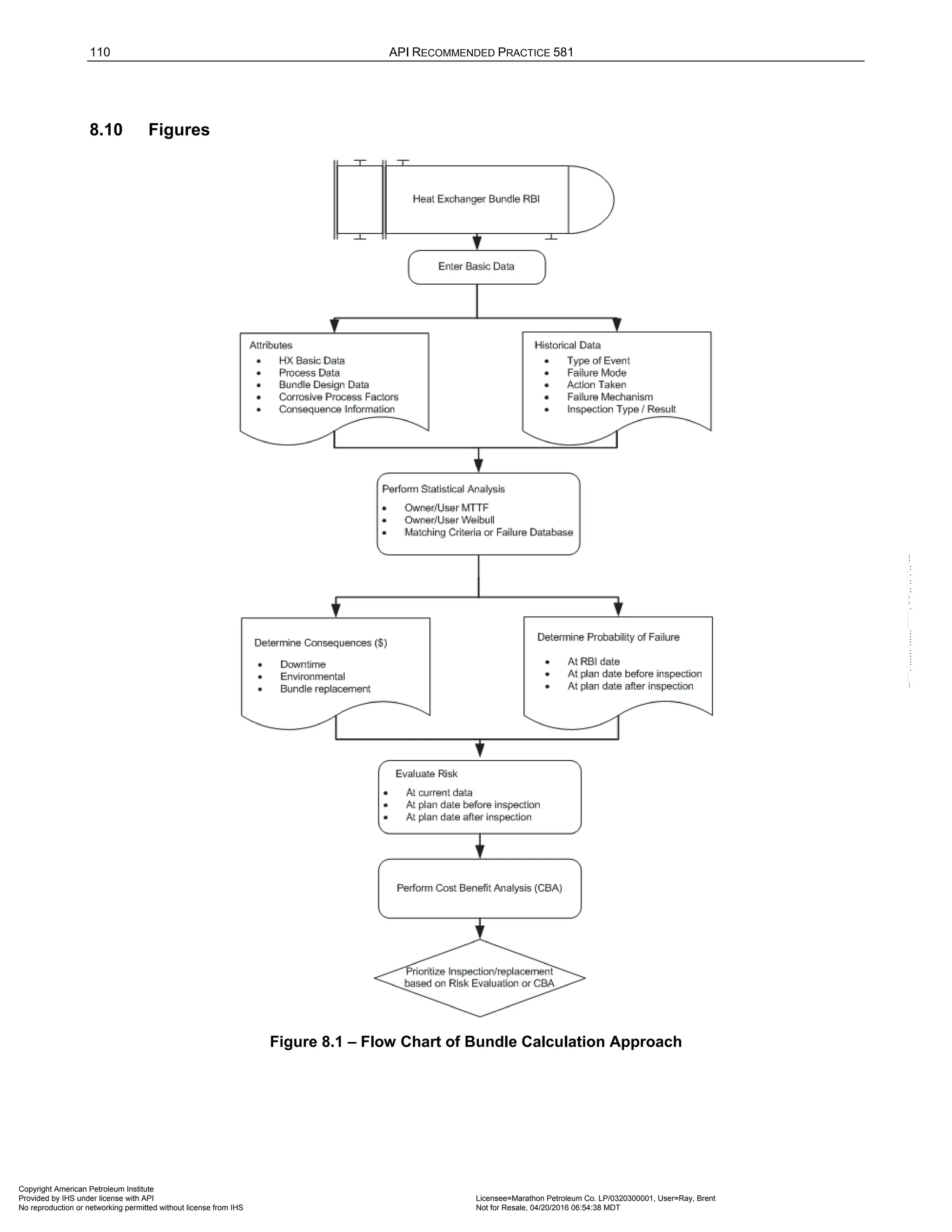
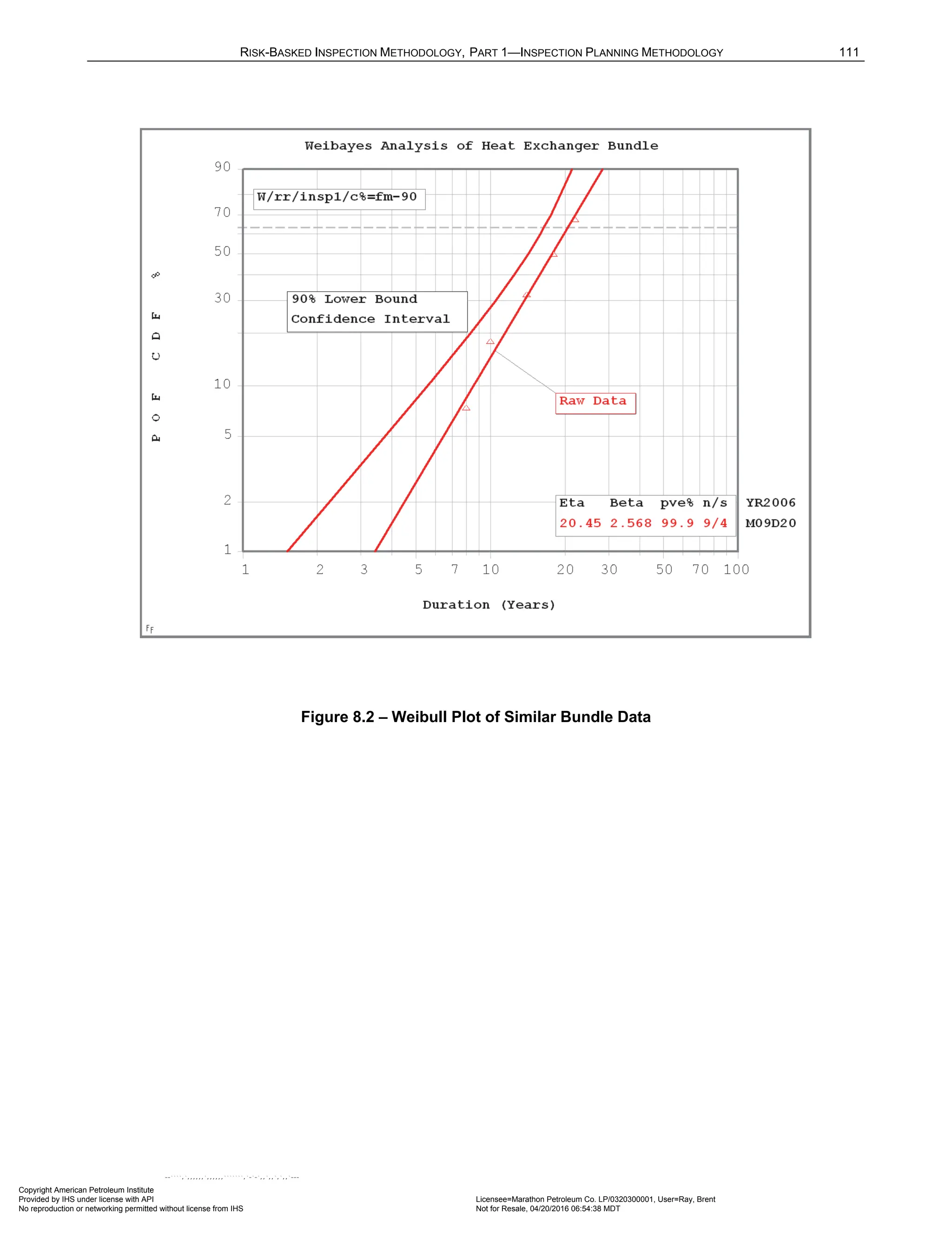
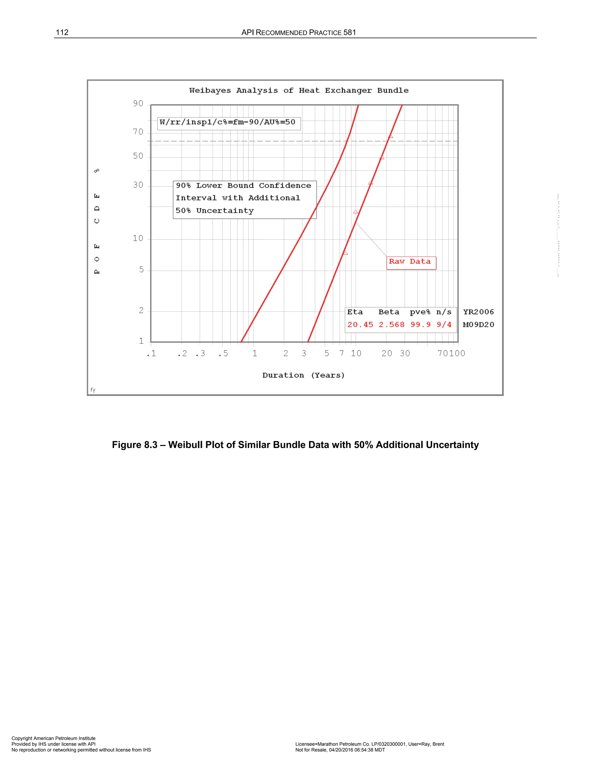
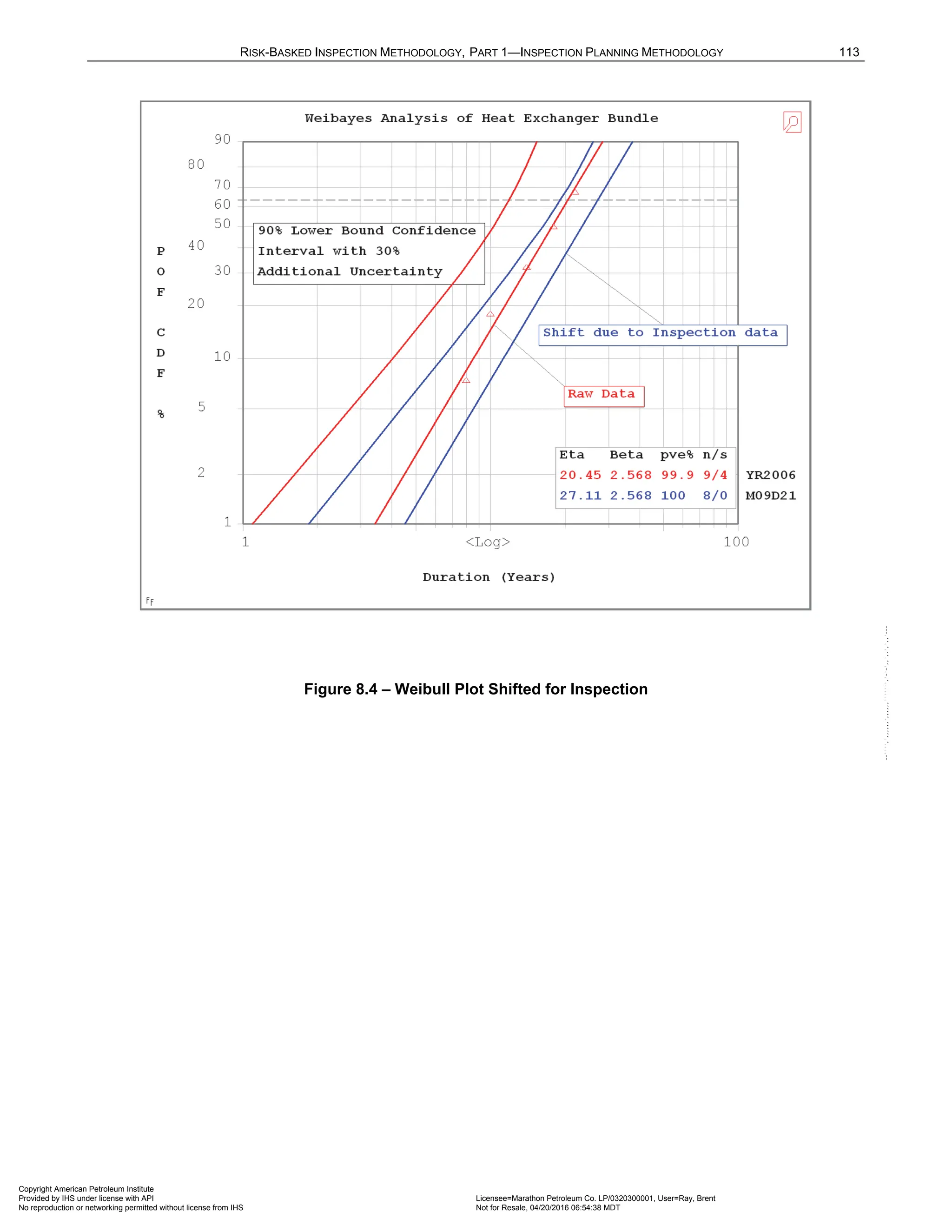
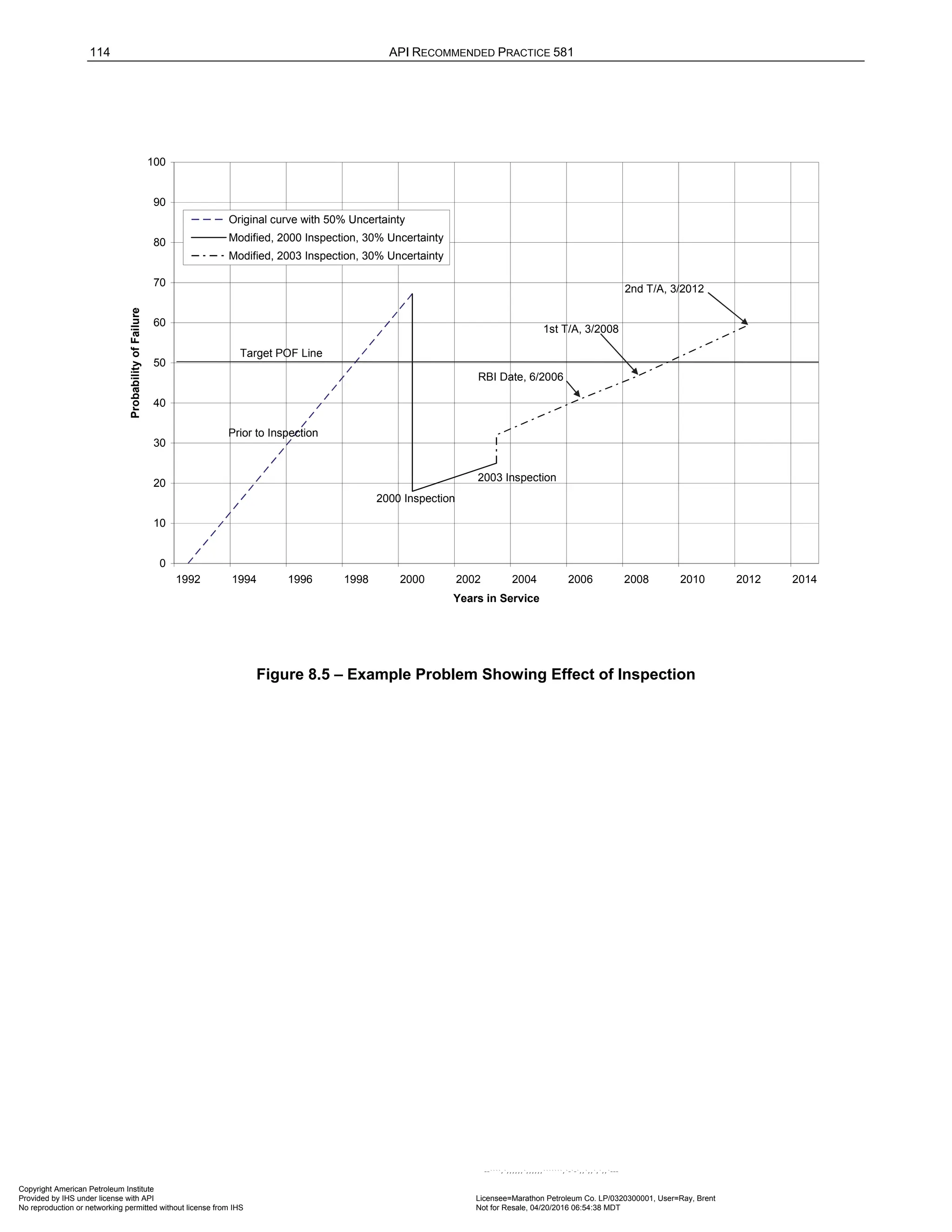
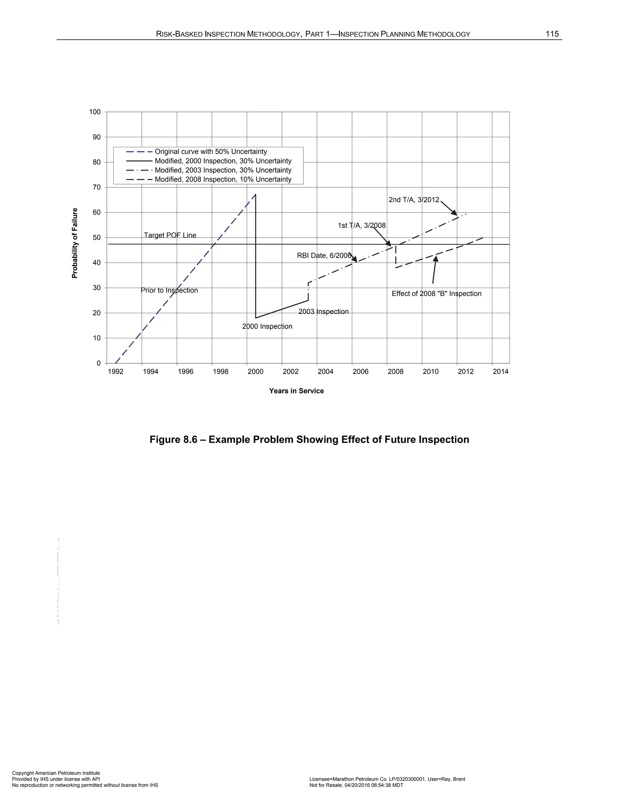


![1
Risk-Based Inspection Methodology
Part 2—Probability of Failure Methodology
1 Scope
The calculation of the probability of failure (POF) of a component is covered in this document. This document is
Part 2 of a three volume set presenting the API RP 581 methodology. The other two Parts are: Part 1 -
Inspection Planning Methodology [15], and Part 3 - Consequence of Failure Methodology [16].
The POF calculated using the methodology in this Part is used with the COF to provide a risk ranking and not
for a rigorous reliability analysis of a component. Alternatively, the POF provided in this Part provides a risk
ranking and inspection plan for a component subject to process and environmental conditions typically found in
the refining, petrochemical industry, exploration and production facilities.
2 References
2.1 Normative
The following referenced documents are indispensable for the application of this document. For dated
references, only the edition cited applies. For undated references, the latest edition of the referenced document
(including any amendments) applies.
2.2 Informative
1. Lees, F.P., Loss Control in the Process Industries, 1980.
2. Smith and Warwick, A Survey of Defects in Pressure Vessels, 1981.
3. US Nuclear Regulatory Commission, WASH-1400, 1970.
4. Thomas, H.M. Pipe and Vessel Failure Probability, Reliability Engineering Journal, 1981.
5. American Petroleum Institute report, Above Ground Storage Tank Survey, by Entropy Limited, 1989.
6. ENI Reliability Databook, Component Reliability Handbook, C. Galvanin, V. Columbari, G. Bellows, Italy,
1982.
7. Nuclear Plant Reliability Data System, Southwest Research Institute, 1981.
8. Krembs, J., Connolly, J., M&M Protection Consultants, Analysis of Large Property Losses in the
Hydrocarbon and Chemical Industries, Refinery and Petrochemical Plant Maintenance Conference, May 23-
25, 1990.
9. Process Safety Management of Highly Hazardous Chemicals. Code of Federal Regulations. Part 1910.119,
Title 29.
10. API, API 579-1/ASME FFS-1 2007 Fitness-For-Service, American Petroleum Institute, Washington, D.C.,
20005, 2007.
11. API, API STD 653 Tank Inspection, Repair, Alteration, And Reconstruction, American Petroleum Institute,
Washington, D.C, 20005.
12. ASME Code, Boiler and Pressure Vessel Code, Section VIII, “Rules For Construction Of Pressure Vessels,”
Division 1.
13. API RP 571 Damage Mechanisms in the Refinery and Petrochemical Industry, American Petroleum
Institute, Washington, D.C.
14. NACE, SP0169 Control of External Corrosion on Underground or Submerged Metallic Piping Systems,
NACE International, Houston, TX.
15. API Recommended Practice 581 Part 1 – Inspection Planning Methodology, American Petroleum Institute,
Washington, D.C.
Copyright American Petroleum Institute
Provided by IHS under license with API Licensee=Marathon Petroleum Co. LP/0320300001, User=Ray, Brent
Not for Resale, 04/20/2016 06:54:38 MDT
No reproduction or networking permitted without license from IHS
--````,`,,,,,,`,,,,,,```````,`-`-`,,`,,`,`,,`---](https://image.slidesharecdn.com/api581-3rdedition-april2016-240227010601-3bf73ab5/75/Norma-API-581-3rd-Edition-April-2016-pdf-134-2048.jpg)
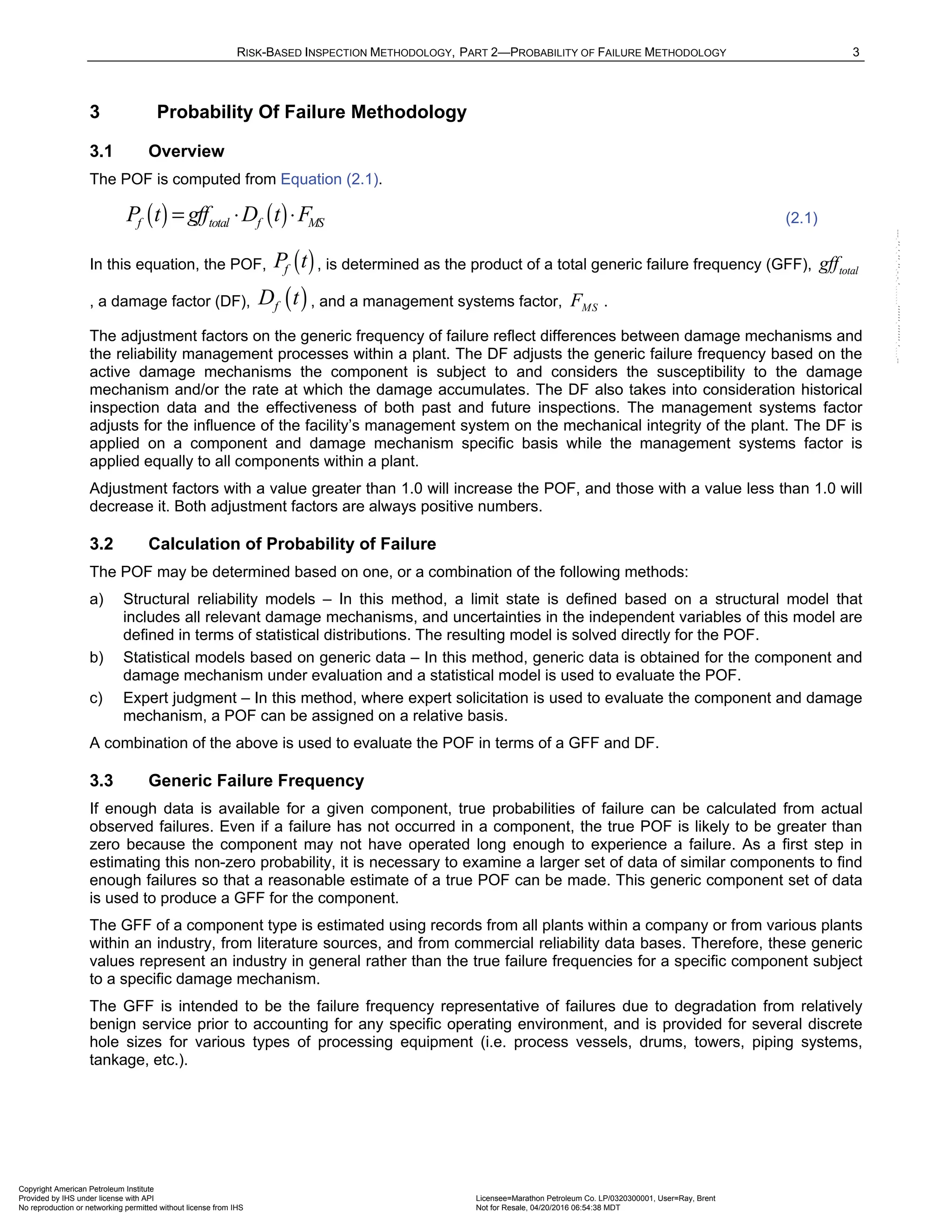
![4 API RECOMMENDED PRACTICE 581
A recommended list of GFFs is provided in Table 3.1 [1 – 8]. The GFFs are assumed to follow a log-normal
distribution, with error rates ranging from 3% to 10%. Median values are given in Table 3.1. The data presented
in the Table 3.1 is based on the best available sources and experience to date from owner-users.
The overall GFF for each component type was divided across the relevant hole sizes, i.e. the sum of the generic
failure frequency for each hole size is equal to the total generic failure frequency for the component.
3.4 Damage Factor
3.4.1 Overview
DFs provide a screening tool to determine inspection priorities and optimize inspection efforts. DFs do not
provide a definitive Fitness-For-Service assessment of the component. The basic function of the DF is to
statistically evaluate the amount of damage that may be present as a function of time in service and the
effectiveness of an inspection activity. DFs are calculated based on the techniques described in Section 3.2, but
are not intended to reflect the actual POF for the purposes of reliability analysis. DFs reflect a relative level of
concern about the component based on the stated assumptions in each of the applicable sections of the
document.
DF estimates are currently provided for the following damage mechanisms.
a) Thinning –
thin
f gov
D −
b) Stress Corrosion Cracking (SCC) –
scc
f gov
D −
c) External Damage –
extd
f gov
D −
d) High Temperature Hydrogen Attack (HTHA) –
htha
f
D
e) Mechanical Fatigue (Piping Only) –
mfat
f
D
f) Brittle Fracture –
brit
f gov
D −
3.4.2 Damage Factor Combination for Multiple Damage Mechanisms
a) Total DF, f total
D −
– If more than one damage mechanism is present, the following rules are used to
combine the DFs. The total DF is given by Equation (2.2) when the external and/or thinning damage are
classified as local and therefore, unlikely to occur at the same location.
max ,
thin extd scc htha brit mfat
f total f gov f gov f gov f f gov f
D D D D D D D
− − − − −
= + + + +
(2.2)
If the external and thinning damage are general, then damage is likely to occur at the same location and
the total DF is given by Equation (2.3).
thin extd scc htha brit mfat
f total f gov f gov f gov f f gov f
D D D D D D D
− − − − −
= + + + + + (2.3)
Note that the summation of DFs can be less than or equal to 1.0. This means that the component can have
a POF less than the generic failure frequency.
b) Governing Thinning DF,
thin
f gov
D − – The governing thinning DF is determined based on the presence of an
internal liner using Equations (2.4) and (2.5).
min ,
thin thin elin
f gov f f
D D D when an internal liner is present
−
= (2.4)
thin thin
f gov f
D D when an internal liner is not present
−
= (2.5)
Copyright American Petroleum Institute
Provided by IHS under license with API Licensee=Marathon Petroleum Co. LP/0320300001, User=Ray, Brent
Not for Resale, 04/20/2016 06:54:38 MDT
No reproduction or networking permitted without license from IHS
--````,`,,,,,,`,,,,,,```````,`-`-`,,`,,`,`,](https://image.slidesharecdn.com/api581-3rdedition-april2016-240227010601-3bf73ab5/75/Norma-API-581-3rd-Edition-April-2016-pdf-137-2048.jpg)
![RISK-BASED INSPECTION METHODOLOGY, PART 2—PROBABILITY OF FAILURE METHODOLOGY 5
c) Governing SCC DF,
scc
f gov
D − – The governing SCC DF is determine from Equation (2.6).
2
/
/
, , , , ,
max
, , ,
HIC SOHIC H S
caustic amine ssc ACSCC
f f f f f
scc
f gov PASCC CLSCC HSC HF HIC SOHIC HF
f f f f
D D D D D
D
D D D D
−
− − −
=
(2.6)
d) Governing External DF,
extd
f gov
D − – The governing external DF is determined from Equation (2.7).
max , , ,
extd extf CUIF ext CLSCC CUI CLSCC
f gov f f f f
D D D D D
− −
−
= (2.7)
e) Governing Brittle Fracture DF,
brit
f gov
D − – The governing brittle fracture DF is determined from Equation
(2.8). When performing the summation of DFs in Equation (2.8), if a DF is less than or equal to one (i.e. the
damage is inactive), then this DF shall be set to zero in the summation.
( )
max , ,
brit brit tempe 885F sigma
f gov f f f f
D D D D D
−
= +
(2.8)
f) A description of the DFs shown above and the associated section number that contains the step-by-step
calculations is provided in Table 3.2.
3.4.3 Inspection Effectiveness Category
DFs are determined as a function of inspection effectiveness. A discussion of inspection effectiveness and
example tables are provided in Annex 2.C. The inspection effectiveness categories are meant to be examples in
order to provide a guideline for the user in assigning actual inspection effectiveness.
The effectiveness of each inspection performed within the designated time period is characterized for each
damage mechanism. The number of inspections and effectiveness of each inspection is used to calculate the
DF. The number and effectiveness of each inspection for thinning and external corrosion is included directly in
the calculation of the DFs (see Sections 4.0, 15.0 and 16.0).
If multiple inspections have been performed, equivalent relationships are used for SCC, External Damage
(external chloride stress corrosion cracking, external chloride stress corrosion cracking under insulation) and
HTHA. Inspections of different grades (A, B, C and D) are approximated as equivalent inspection effectiveness
in accordance with the following relationships:
a) 2 Usually Effective (B) Inspections = 1 Highly Effective (A) Inspection, or 2B = 1A
b) 2 Fairly Effective (C) Inspections = 1 Usually Effective (B) inspection, or 2C = 1B
c) 2 Poorly Effective (D) Inspections = 1 Fairly Effective (C) inspection, or 2D = 1C
Note:
1. Equivalent inspection valuesare not used for Thinning and External Corrosion DF calculations.
2. The equivalent higher inspection rules shall not be applied to No Inspections (E).
3.5 Management Systems Factor
3.5.1 General
The effectiveness of a company’s process safety management system can have a pronounced effect on
mechanical integrity. The methodology includes an evaluation tool to assess the portions of the facility’s
management system that most directly impact the POF of a component. This evaluation consists of a series of
interviews with plant management, operations, inspection, maintenance, engineering, training, and safety
personnel. The importance of an effective management system evaluation has long been recognized in
preventing releases of hazardous materials and maintaining the mechanical integrity of process equipment.
Compliance with PSM standards became mandatory in the United States in 1992 with the issue of OSHA 29
CFR 1910.119 [9].
Copyright American Petroleum Institute
Provided by IHS under license with API Licensee=Marathon Petroleum Co. LP/0320300001, User=Ray, Brent
Not for Resale, 04/20/2016 06:54:38 MDT
No reproduction or networking permitted without license from IHS
--````,`,,,,,,`,,,,,,```````,`-`-`,,`,,`,`,,`---](https://image.slidesharecdn.com/api581-3rdedition-april2016-240227010601-3bf73ab5/75/Norma-API-581-3rd-Edition-April-2016-pdf-138-2048.jpg)
![RISK-BASED INSPECTION METHODOLOGY, PART 2—PROBABILITY OF FAILURE METHODOLOGY 7
The intent of the management systems evaluation is to arrive at the single best answer for each question. In
addition to comparing answers from different interviews, many of the responses should be verified by physical
review of the appropriate written procedures, files and records. The auditor must ensure that the facts
substantiate the answer, and that the intent of the question is met before credit is awarded for the answer.
3.5.4 Calculation of the Management Systems Factor
The scale recommended for converting a management systems evaluation score to a management systems
factor is based on the assumption that the “average” plant would score 50% (500 out of a possible score of
1,000) on the management systems evaluation, and that a 100% score would equate to a one order-of-
magnitude reduction in total unit risk. Based on this ranking, Equations (2.9) and (2.10) are used to compute a
management systems factor, MS
F , for any management systems evaluation score, Score . Note that the
management score must first be converted to a percentage (between 0 and 100) as follows:
[ ]
100 unit is %
1000
Score
pscore = ⋅ (2.9)
( )
0.02 1
10 pscore
MS
F − ⋅ +
= (2.10)
The above assumptions can be modified and improved over time as more data become available on
management systems evaluation results.
It should be remembered that the management systems factor applies equally to all components and therefore,
does not change the risk ranking of components for inspection prioritization. The factor’s value is in comparing
one operating unit or plant site to another.
3.6 Nomenclature
f
D for each mechanism and relevant section references are outlined in Table 3.2.
( )
f
D t is the DF as a function of time, equal to f total
D −
evaluated at a specific time
ACSCC
f
D is the DF for alkaline carbonate stress corrosion cracking (ACSCC)
amine
f
D is the DF for amine cracking
brit
f gov
D − is the governing DF for brittle fracture
brit
f
D is the DF for brittle fracture
caustic
f
D is the DF for caustic cracking
CLSCC
f
D is the DF for chloride stress corrosion cracking (CLSCC)
CUIF
f
D is the DF for corrosion under insulation (CUI) for ferritic components
CUI CLSCC
f
D −
is the DF for corrosion under insulation CUI) for austenitic stainless steel components subject to
external chloride stress corrosion cracking
extd
f gov
D − is the governing DF for external damage
extcor
f
D is the DF for external corrosion
Copyright American Petroleum Institute
Provided by IHS under license with API Licensee=Marathon Petroleum Co. LP/0320300001, User=Ray, Brent
Not for Resale, 04/20/2016 06:54:38 MDT
No reproduction or networking permitted without license from IHS
--````,`,,,,,,`,,,,,,```````,`-`-`,,`,,`,`,,`---](https://image.slidesharecdn.com/api581-3rdedition-april2016-240227010601-3bf73ab5/75/Norma-API-581-3rd-Edition-April-2016-pdf-140-2048.jpg)
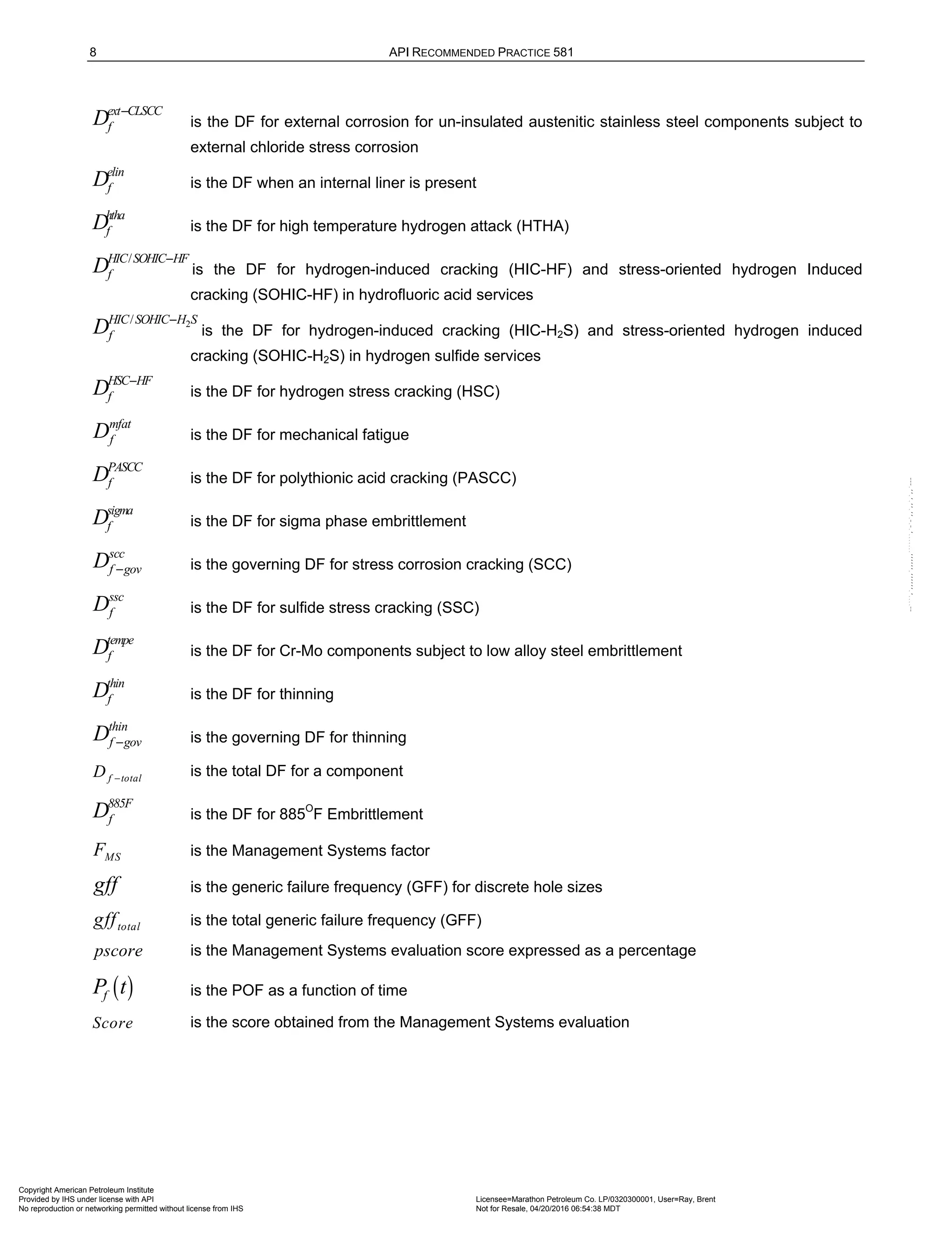
![RISK-BASED INSPECTION METHODOLOGY, PART 2—PROBABILITY OF FAILURE METHODOLOGY 9
3.7 Tables
Table 3.1 – Suggested Component Generic Failure Frequencies
Equipment Type
Component
Type
gff as a Function of Hole Size (failures/yr) total
gff
(failures/yr)
Small Medium Large Rupture
Compressor COMPC 8.00E-06 2.00E-05 2.00E-06 0 3.00E-05
Compressor COMPR 8.00E-06 2.00E-05 2.00E-06 6.00E-07 3.06E-05
Heat Exchanger
HEXSS.
HEXTS,
8.00E-06 2.00E-05 2.00E-06 6.00E-07 3.06E-05
Pipe PIPE-1,
PIPE-2
2.80E-05 0 0 2.60E-06 3.06E-05
Pipe PIPE-4,
PIPE-6
8.00E-06 2.00E-05 0 2.60E-06 3.06E-05
Pipe
PIPE-8,
PIPE-10,
PIPE-12,
PIPE-16,
PIPEGT16
8.00E-06 2.00E-05 2.00E-06 6.00E-07 3.06E-05
Pump
PUMP2S,
PUMPR,
PUMP1S
8.00E-06 2.00E-05 2.00E-06 6.00E-07 3.06E-05
Tank650 TANKBOTTOM 7.20E-04 0 0 2.00E-06 7.20E-04
Tank650 COURSE-1-10 7.00E-05 2.50E-05 5.00E-06 1.00E-07 1.00E-04
Vessel/FinFan
KODRUM,
COLBTM,
FINFAN,
FILTER,
DRUM,
REACTOR,
COLTOP,
COLMID
8.00E-06 2.00E-05 2.00E-06 6.00E-07 3.06E-05
Note:
See references [1] through [8] for discussion of failure frequencies for equipment
Copyright American Petroleum Institute
Provided by IHS under license with API Licensee=Marathon Petroleum Co. LP/0320300001, User=Ray, Brent
Not for Resale, 04/20/2016 06:54:38 MDT
No reproduction or networking permitted without license from IHS
--````,`,,,,,,`,,,,,,```````,`-`-`,,`,,`,`,,`---](https://image.slidesharecdn.com/api581-3rdedition-april2016-240227010601-3bf73ab5/75/Norma-API-581-3rd-Edition-April-2016-pdf-142-2048.jpg)
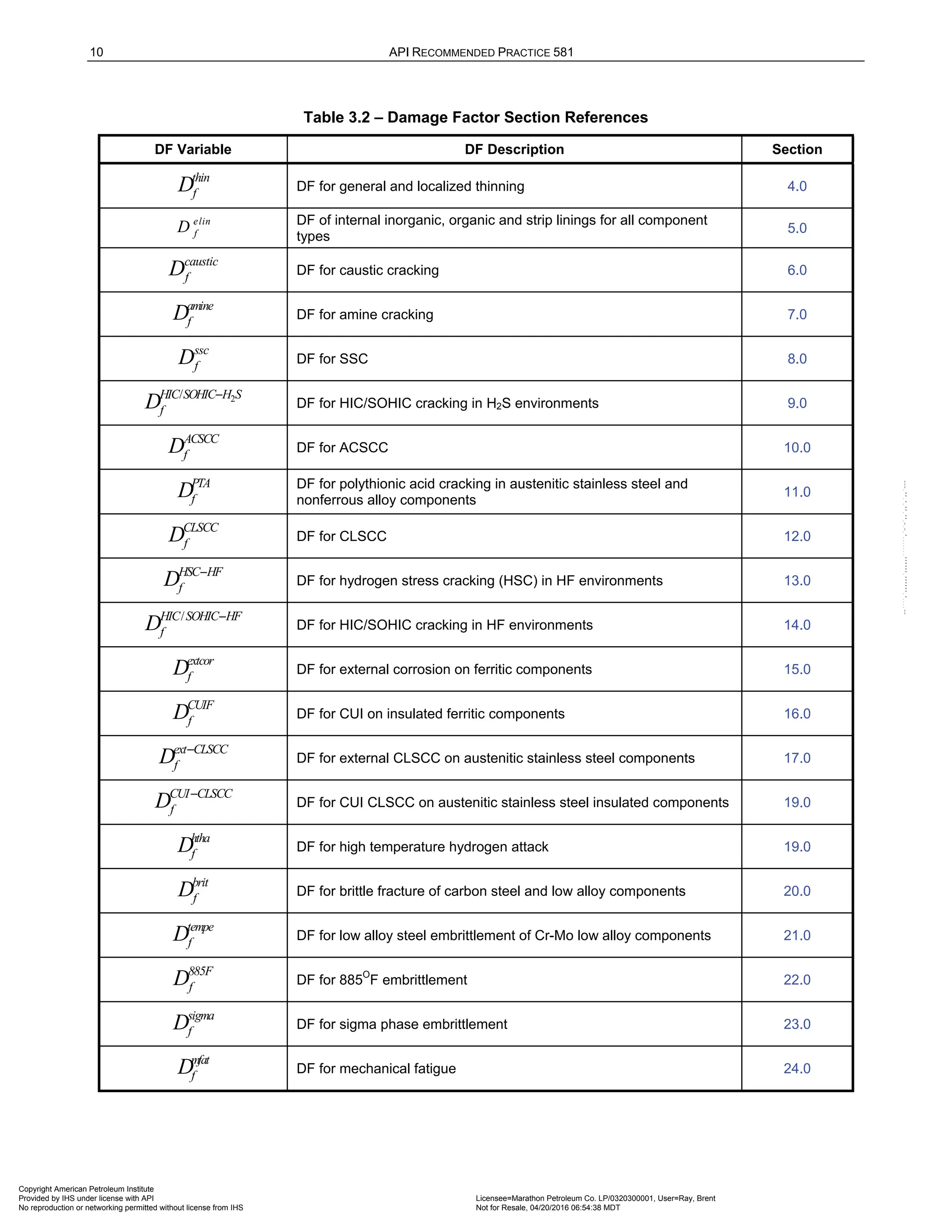
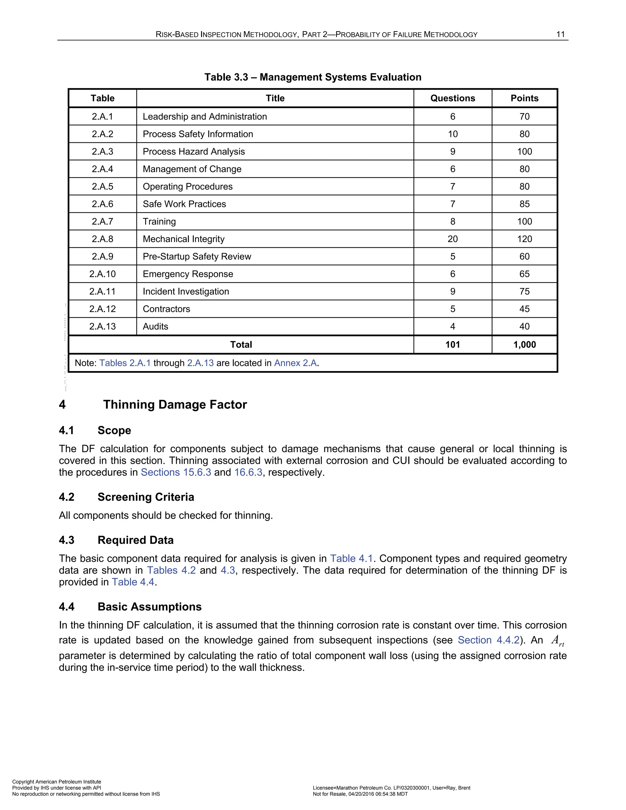
![14 API RECOMMENDED PRACTICE 581
4.5.6 Inspection Effectiveness
Inspections are ranked according to their expected effectiveness at detecting thinning and correctly predicting
the rate of thinning. Table 4.6 provides the conditional probabilities for each inspection effectiveness category in
the thinning DF calculations. These probabilities are used with the three damage states and Bayes Theorem
described in Section 4.5.3. The actual effectiveness of a given inspection technique depends on the
characteristics of the thinning mechanism, (i.e., whether it is general or localized).
Examples of inspection activities for specific applications are provided in Annex 2.C for:
a) General and localized thinning that are either intrusive or non-intrusive in Tables 2.C.8.1 and 2.C.8.2
b) Buried components in Table 2.C.7.1
c) General and localized thinning applied to Atmospheric Storage Tank (AST) shell courses and bottoms in
Tables 2.C.5.1 through 2.C.5.3.
For localized thinning, selection of locations for examination must be based on a thorough understanding of the
damage mechanism in the specific process.
The effectiveness of each inspection performed within the designated time period must be characterized in a
manner similar to the examples provided in Annex 2.C, as applicable. The number and effectiveness of each
inspection is used to determine the DF. Inspection performed prior to the designated time period are typically
not used to determine the DF.
Note that for AST bottoms, credit is given for only one inspection.
4.5.7 Calculation of Thinning Damage Factor
The following procedure may be used to determine the DF for thinning, see Figure 4.1. Note that this procedure
assumes that if cladding/weld overlay is present, it corrodes prior to any corrosion of the base material.
a) STEP 1 – Determine the furnished thickness, t , and age, age , for the component from the installation
date.
b) STEP 2 – Determine the corrosion rate for the base material, ,
r bm
C , based on the material of construction
and process environment, using guidance from Section 4.5.2 and examples in Annex 2.B for establishing
corrosion rates. For a component with cladding/weld overlay, the cladding/weld overlay corrosion rate,
,
r cm
C , must be determined.
c) STEP 3 – Determine the time in service, tk
age , since the last inspection known thickness , rdi
t . The rdi
t is
the starting thickness with respect to wall loss associated with internal corrosion (see Section 4.5.5). If no
measured thickness is available, set rdi
t t
= and tk
age age
= .
d) STEP 4 – For cladding/weld overlay pressure vessel components, calculate the age from the date of the
the starting thickness from STEP 3 required to corrode away the cladding/weld overlay material, rc
age ,
using Equation (2.11).
,
)
max , 0.0
rdi bm
rc
r cm
t t
age
C
−
=
(2.11)
e) STEP 5 – Determine min
t using one of the following methods:
1) For cylindrical, spherical or head components, determine the allowable stress, S , weld joint efficiency,
E , and calculate the minimum required thickness, min
t , using component type in Table 4.2, geometry
type in Table 4.3 and per the original construction code or API 579-1/ASME FFS-1 [10].
2) In cases where components are constructed of uncommon shapes or where the component's minimum
structural thickness, c
t , may govern, the user may use the c
t in lieu of min
t .
Copyright American Petroleum Institute
Provided by IHS under license with API Licensee=Marathon Petroleum Co. LP/0320300001, User=Ray, Brent
Not for Resale, 04/20/2016 06:54:38 MDT
No reproduction or networking permitted without license from IHS
--````,`,,,,,,`,,,,,,```````,`-`-`,,`,,`,`,,`---](https://image.slidesharecdn.com/api581-3rdedition-april2016-240227010601-3bf73ab5/75/Norma-API-581-3rd-Edition-April-2016-pdf-147-2048.jpg)
![RISK-BASED INSPECTION METHODOLOGY, PART 2—PROBABILITY OF FAILURE METHODOLOGY 15
3) If the component is a tank bottom, use min 0.1
t in
= if the AST does not have a release prevention
barrier or min 0.05
t in
= if the AST has a release prevention barrier, in accordance with API STD 653
[11].
4) A specific min
t calculated by another method and documented in the asset management program may
be used at the owner-user's discretion.
f) STEP 6 - Determine the rt
A parameter using Equation (2.12), (2.13), (2.14) or (2.15), as appropriate,
based on t from STEP 1, ,
r bm
C and ,
r cm
C from STEP 2, tk
age and rdi
t from STEP 3, and the age
required to corrode away the cladding/weld overlay, rc
age , if applicable, from STEP 4. Note that the age
parameter in these equations is equal to tk
age from STEP 3.
1) For tank bottom components, calculate the rt
A parameter using Equation (2.12) and skip to STEP 13.
,
min
( )
max 1 , 0.0
rdi r bm tk
rt
t C age
A
t CA
− ⋅
= −
+
(2.12)
2) For components without cladding/weld overlay or where the cladding/weld overlay is corroded away at the
date of the starting thickness from STEP 2, i.e. 0.0
rc
age = , use Equation (2.13).
,
r bm tk
rt
rdi
C age
A
t
⋅
= (2.13)
3) For components with cladding/weld overlay (i.e. 0.0
rc
age ≥ ) at the date of the starting thickness from
STEP 2 but where tk rc
age age
< , use Equation (2.14):
,
r cm tk
rt
rdi
C age
A
t
⋅
= (2.14)
4) For components with cladding/weld overlay (i.e. 0.0
rc
age ≥ ) at the date of the starting thickness STEP 2
inspection but where tk rc
age age
≥ , use Equation (2.15):
( )
, ,
r cm rc r bm tk rc
rt
rdi
C age C age age
A
t
⋅ + ⋅ −
= (2.15)
g) STEP 7 – Calculate the Flow Stress, Thin
FS , using E from STEP 5 and Equation (2.16).
( ) 1.1
2
Thin YS TS
FS E
+
= ⋅ ⋅ (2.16)
Note: Use Flow Stress ( Thin
FS ) at design temperature for conservative results, using the appropriate
Equation (2.17) or (2.18).
h) STEP 8 – Calculate the strength ratio parameter, Thin
P
SR , using the appropriate Equation (2.17) or (2.18).
Using Equation (2.17) with rdi
t from STEP 3, min
t or c
t from STEP 5, S , and E from STEP 5, and flow
stress, Thin
FS , from STEP 7.
Copyright American Petroleum Institute
Provided by IHS under license with API Licensee=Marathon Petroleum Co. LP/0320300001, User=Ray, Brent
Not for Resale, 04/20/2016 06:54:38 MDT
No reproduction or networking permitted without license from IHS
--````,`,,,,,,`,,,,,,```````,`-`-`,,`,,`,`,,`---](https://image.slidesharecdn.com/api581-3rdedition-april2016-240227010601-3bf73ab5/75/Norma-API-581-3rd-Edition-April-2016-pdf-148-2048.jpg)
![RISK-BASED INSPECTION METHODOLOGY, PART 2—PROBABILITY OF FAILURE METHODOLOGY 17
l) STEP 12 – Calculate the parameters, 1 2 3
, ,
Thin Thin Thin
β β β using Equation (2.21) and assigning 0.20
t
COVΔ =
, 0.20
f
S
COV = and 0.05
P
COV = .
( )
( )
1
1 1
2
2 2
3
3 3
1 2
2 2 2 2 2 2
2 2
2 2 2 2 2 2
3
2 2 2
1
,
1 ( )
1
,
1 ( )
1
1
f
f
Thin
S rt p
Thin
Thin
S rt t S rt S p P
Thin
S rt p
Thin
Thin
S rt t S rt S p P
Thin
S rt p
Thin
S rt t S
D A SR
D A COV D A COV SR COV
D A SR
D A COV D A COV SR COV
D A SR
D A COV D A
β
β
β
Δ
Δ
Δ
− ⋅ −
=
⋅ ⋅ + − ⋅ ⋅ + ⋅
− ⋅ −
=
⋅ ⋅ + − ⋅ ⋅ + ⋅
− ⋅ −
=
⋅ ⋅ + − ⋅
( )
2
2 2 2
.
( )
f
Thin
rt S p P
COV SR COV
⋅ + ⋅
(2.21)
Where 1
1
S
D = , 2
2
S
D = and 3
4
S
D = . These are the corrosion rate factors for damage states 1, 2 and 3 as as
discussed in Section 4.5.3 [35]. Note that the DF calculation is very sensitive to the value used for the coefficient
of variance for thickness, t
COVΔ . The t
COVΔ is in the range 0.10 0.20
t
COVΔ
≤ ≤ , with a recommended
conservative value of 0.20
t
COVΔ = .
m) STEP 13 – For tank bottom components, determine the base damage factor for thinning, thin
fB
D , using Table
4.8 and based on the rt
A parameter from STEP 6 and Skip to STEP 15.
n) STEP 14 – For all components (excluding tank bottoms covered in STEP 13), calculate the base damage
factor,
Thin
fB
D .
( )
( ) ( )
( ) ( )
( )
1 1 2 2 3 3
1.56 04
Thin Thin Thin Thin Thin Thin
p p p
Thin
fb
Po Po Po
D
E
β β β
Φ − + Φ − + Φ −
=
−
(2.22)
Where Φ is the standard normal cumulative distribution function (NORMSDIST in Excel).
o) STEP 15 – Determine the DF for thinning,
Thin
f
D , using Equation (2.23).
max , 0.1
Thin
fB IP DL WD AM SM
Thin
f
OM
D F F F F F
D
F
⋅ ⋅ ⋅ ⋅ ⋅
=
(2.23)
The adjustment factors in are determined as described below.
1) Adjustment to DF for On-Line Monitoring, OM
F – In addition to inspection, on-line monitoring of corrosion
(or key process variables affecting corrosion) is commonly used in many processes to prevent corrosion
failures. The advantage of on-line monitoring is that changes in corrosion rates as a result of process
changes can be detected long before they would be detected with normal periodic inspections. This earlier
detection usually permits more timely action to be taken that should decrease the POF. Various methods
are employed, ranging from corrosion probes, corrosion coupons, and monitoring of key process variables.
If on-line monitoring is employed, then credit should be given to reflect higher confidence in the predicted
thinning rate. However, these methods have a varying degree of success depending on the specific thinning
mechanism. Using knowledge of the thinning mechanism and the type of on-line monitoring, determine the
on-line monitoring factor from Table 4.9. If more than one monitoring method is used, only the highest
monitoring factor should be used (i.e. the factors are not additive).
Copyright American Petroleum Institute
Provided by IHS under license with API Licensee=Marathon Petroleum Co. LP/0320300001, User=Ray, Brent
Not for Resale, 04/20/2016 06:54:38 MDT
No reproduction or networking permitted without license from IHS
--````,`,,,,,,`,,,,,,```````,`-`-`,,`,,`,`,,`---](https://image.slidesharecdn.com/api581-3rdedition-april2016-240227010601-3bf73ab5/75/Norma-API-581-3rd-Edition-April-2016-pdf-150-2048.jpg)
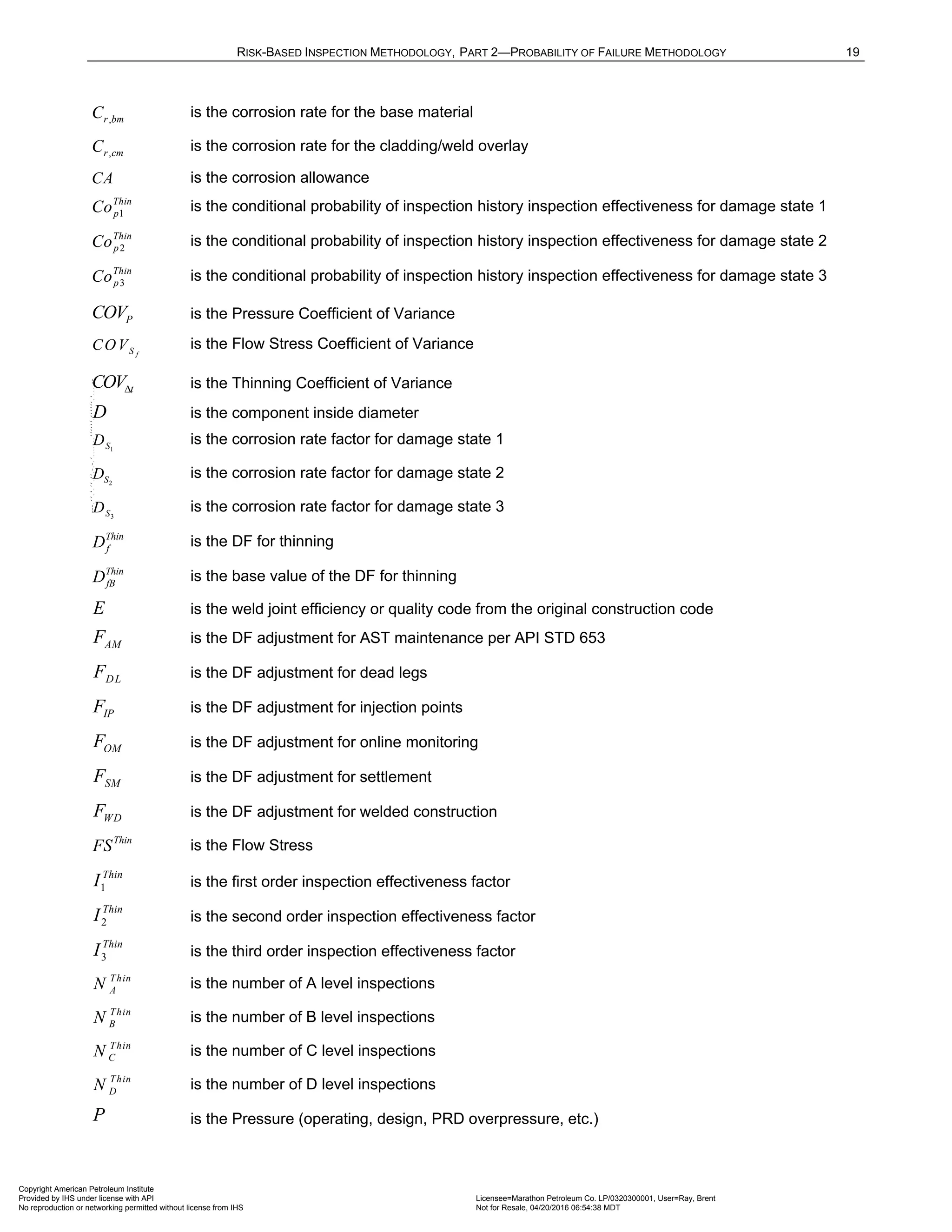

![RISK-BASED INSPECTION METHODOLOGY, PART 2—PROBABILITY OF FAILURE METHODOLOGY 21
4.7 Tables
Table 4.1 – Basic Component Data Required for Analysis
Basic Data Comments
Start Date The date the component was placed in service.
Thickness, mm (inch) The thickness used for the DF calculation that is either the furnished thickness or
the measured thickness (See Section 4.5.5).
Corrosion Allowance,
mm [inch]
The corrosion allowance is the specified design or actual corrosion allowance upon
being placed in the current service.
Design Temperature, °C (°F) The design temperature, shell side and tube side for a heat exchanger.
Design Pressure, MPa (psi) The design pressure, shell side and tube side for a heat exchanger.
Operating Temperature,
°C (°F)
The highest expected operating temperature expected during operation including
normal and unusual operating conditions, shell side and tube side for a heat
exchanger.
Operating Pressure,
MPa (psi)
The highest expected operating pressure expected during operation including normal
and unusual operating conditions, shell side and tube side for a heat exchanger.
Design Code The design code of the component containing the component.
Equipment Type The type of Equipment.
Component Type The type of Component, see Table 4.2.
Component Geometry Data Component geometry data depending on the type of component (see Table 4.3).
Material Specification The specification of the material of construction, the ASME SA or SB specification for
pressure vessel components or of ASTM specification for piping and tankage
components. Data entry is based on material specification, grade, year, UNS Number,
class/condition/temper/ size/thickness; this data is readily available in the ASME Code
[12].
Yield Strength, MPa (psi) The design yield strength of the material based on material specification.
Tensile Strength, MPa (psi) The design tensile strength of the material based on material specification.
Weld Joint Efficiency Weld joint efficiency per the Code of construction,
Heat Tracing Is the component heat traced? (Yes or No)
Copyright American Petroleum Institute
Provided by IHS under license with API Licensee=Marathon Petroleum Co. LP/0320300001, User=Ray, Brent
Not for Resale, 04/20/2016 06:54:38 MDT
No reproduction or networking permitted without license from IHS
--````,`,,,,,,`,,,,,,```````,`-`-`,,`,,`,`,,`---](https://image.slidesharecdn.com/api581-3rdedition-april2016-240227010601-3bf73ab5/75/Norma-API-581-3rd-Edition-April-2016-pdf-154-2048.jpg)
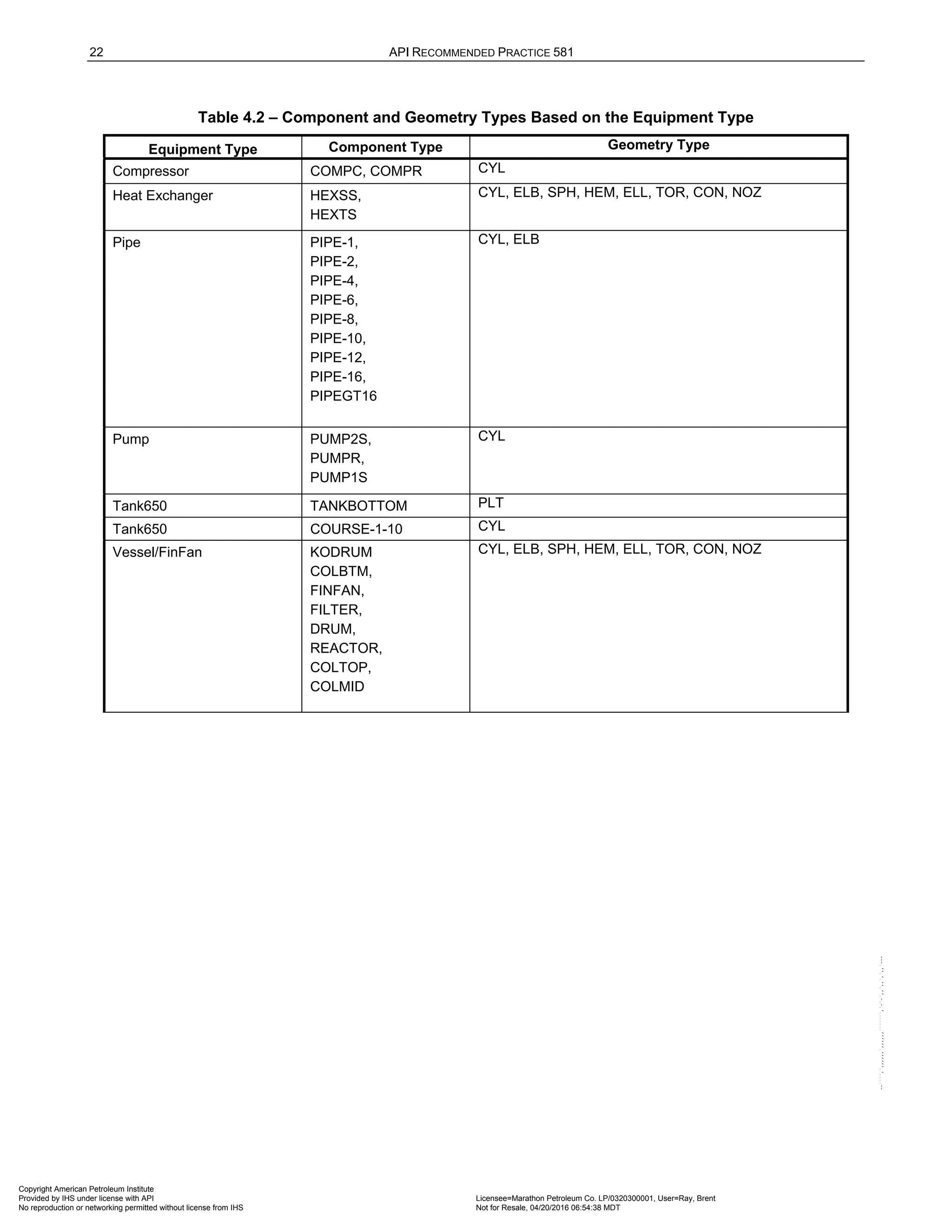
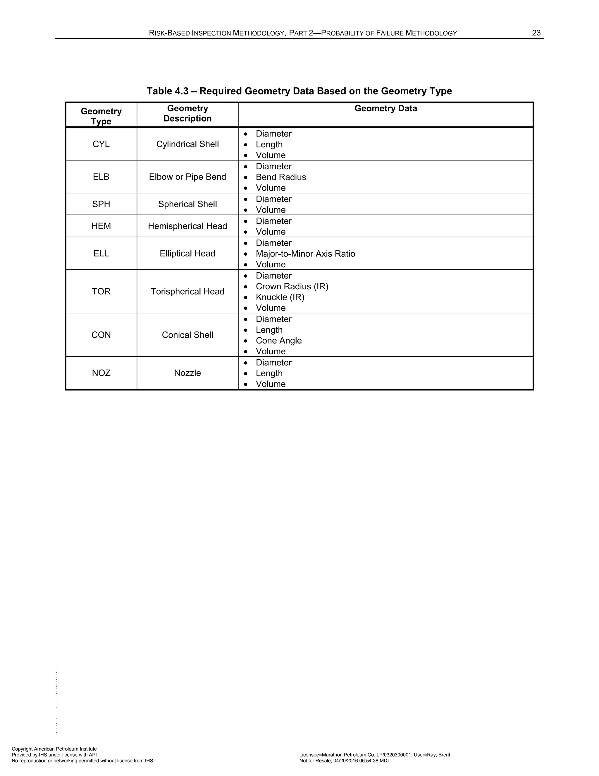
![24 API RECOMMENDED PRACTICE 581
Table 4.4 – Data Required for Determination of the Thinning Damage Factor
Basic Data Comments
Thinning Type
(General or Localized)
Determine whether the thinning is general or localized based on inspection results of
effective inspections. General corrosion is defined as affecting more than 10% of the
surface area and the wall thickness variation is less than 1.27 mm (50 mils). Localized
corrosion is defined as affecting less than 10% of the surface area or a wall thickness
variation greater than 1.27 mm (50 mils).
Corrosion Rate
(mmpy or mpy)
The current rate of thinning calculated from thickness data, if available. Corrosion
rates calculated from thickness data typically vary from one inspection to another.
These variations may be due to variations in the wall thickness, or they may indicate a
change in the actual corrosion rate. If the short-term rate (calculated from the
difference between the current thickness and the previous thickness) is significantly
different from the long-term rate (calculated from the difference between the current
thickness and the original thickness), then the component may be evaluated using the
short term rate, but the appropriate time and thickness must be used.
Inspection Effectiveness
Category
The effectiveness category of each inspection that has been performed on the
component during the time period (specified above).
Number of Inspections The number of inspections in each effectiveness category that have been performed
during the time period (specified above).
On-Line Monitoring The types of proactive on-line monitoring methods or tools employed, such as
corrosion probes, coupons, process variables (Coupons, Probes, Process Variables,
or Combinations, etc.)
Thinning Mechanism If credit is to be taken for on-line monitoring, the potential thinning mechanisms must
be known. A knowledgeable materials/corrosion engineer should be consulted for this
information, also see API RP 571 [13].
Presence of Injection/Mix Point
(Yes or No).
For piping, determine if there is an injection or mix point in the circuit.
Type of Injection/Mix Point
Inspection
For piping circuits which contain an injection or mix point, determine whether
not the inspection program is highly effective or not highly effective to detect local
corrosion at these points.
Presence of a Deadleg
(Yes or No).
For piping, determine if there is a deadleg in the circuit.
Type of Inspection for Deadleg
Corrosion
For piping circuits which contain a deadleg, determine if the inspection program
currently being used is highly effective or not highly effective to detect local corrosion
in dead legs has been performed.
Welded Construction Applicable to ASTs only, ASTs may be welded or riveted construction. Is the AST of
welded construction? (Yes or No)
Maintained to API STD 653 Applicable to ASTs only. Is the AST maintained in accordance with API STD 653
[11]? (Yes or No)
Settlement Applicable to ASTs only, ASTs may be welded or riveted construction. What is the
settlement history of the AST
• Recorded settlement exceeds API STD 653 criteria
• Recorded settlement meets API STD 653 criteria
• Settlement never evaluated
• Concrete foundation, no settlement
Copyright American Petroleum Institute
Provided by IHS under license with API Licensee=Marathon Petroleum Co. LP/0320300001, User=Ray, Brent
Not for Resale, 04/20/2016 06:54:38 MDT
No reproduction or networking permitted without license from IHS
--````,`,,,,,,`,,,,,,```````,`-`-`,,`,,`,`,,`---](https://image.slidesharecdn.com/api581-3rdedition-april2016-240227010601-3bf73ab5/75/Norma-API-581-3rd-Edition-April-2016-pdf-157-2048.jpg)
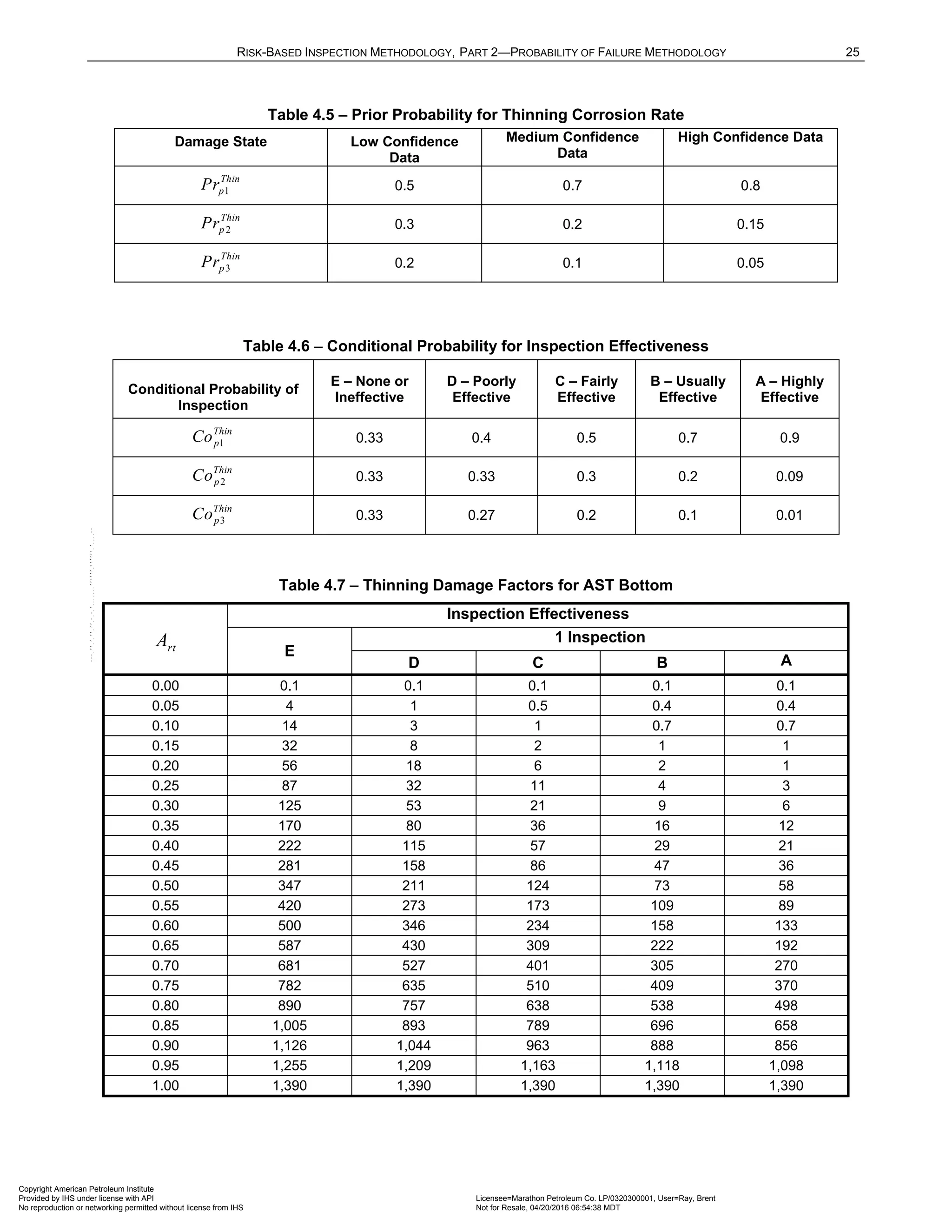
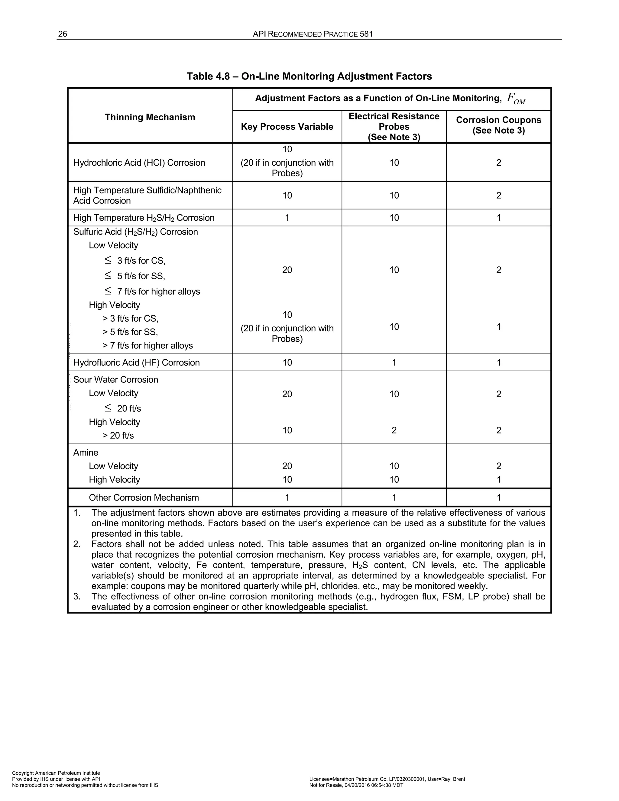
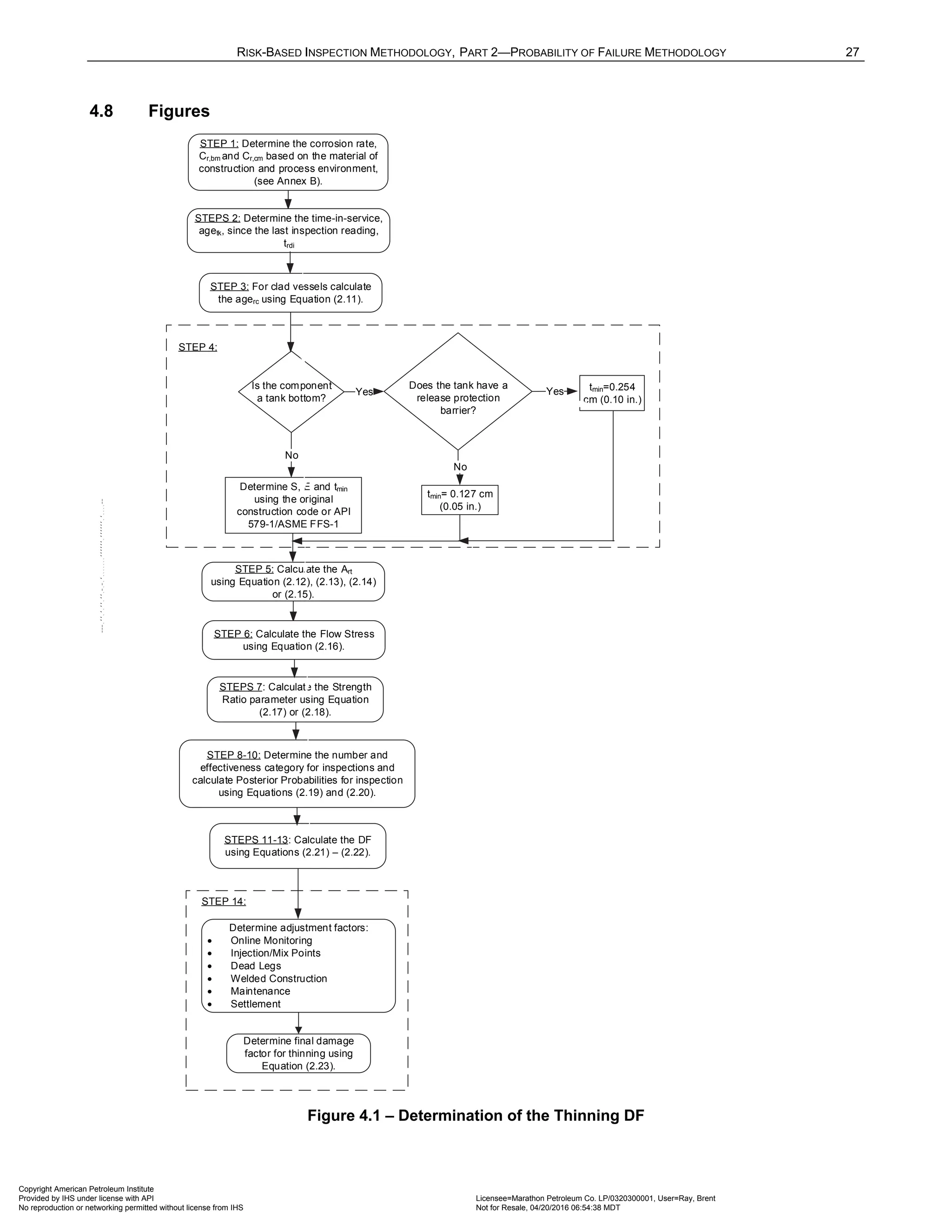
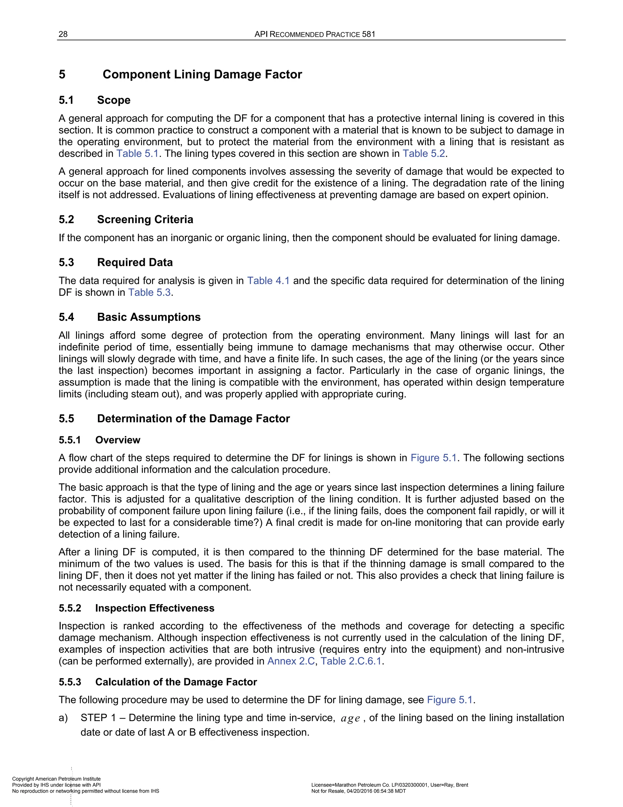
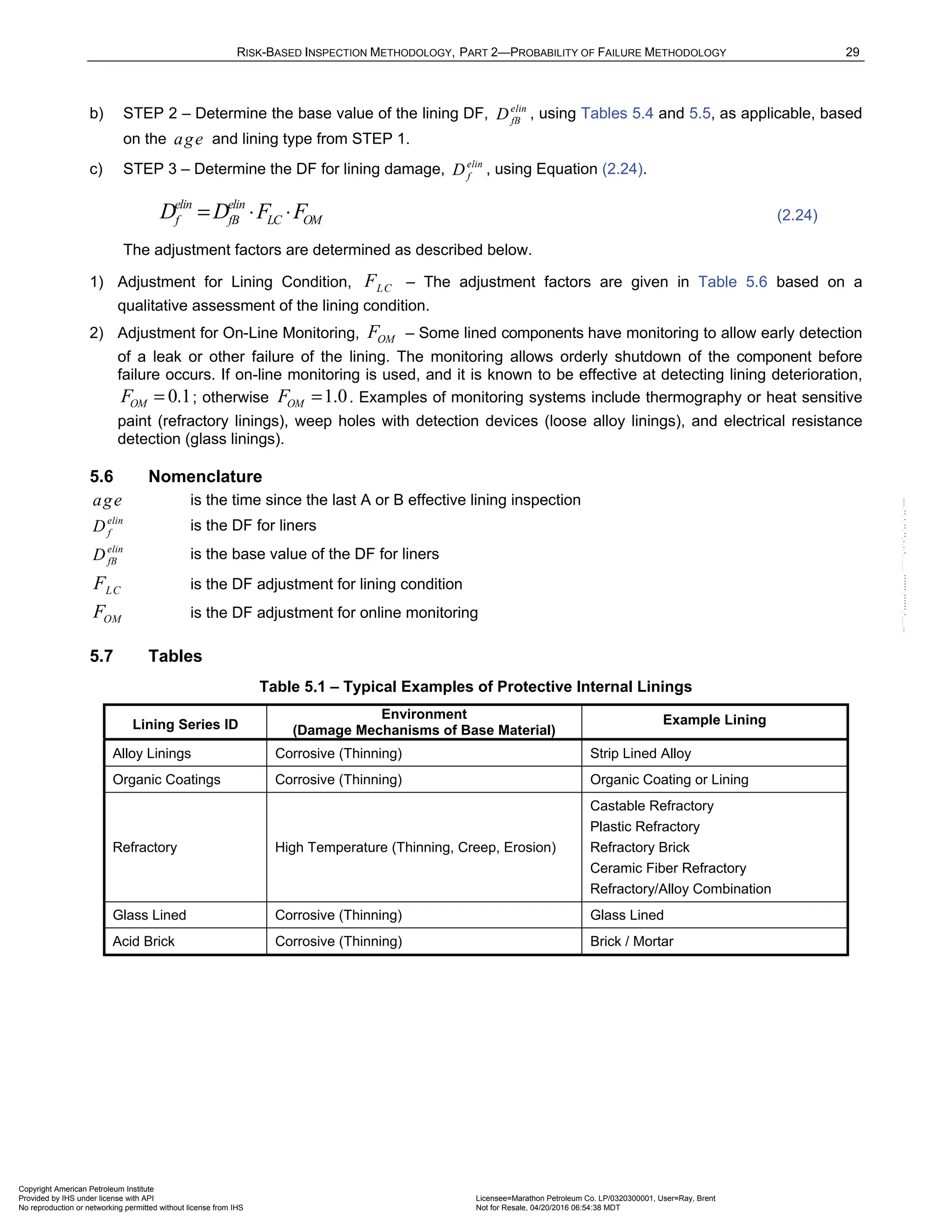
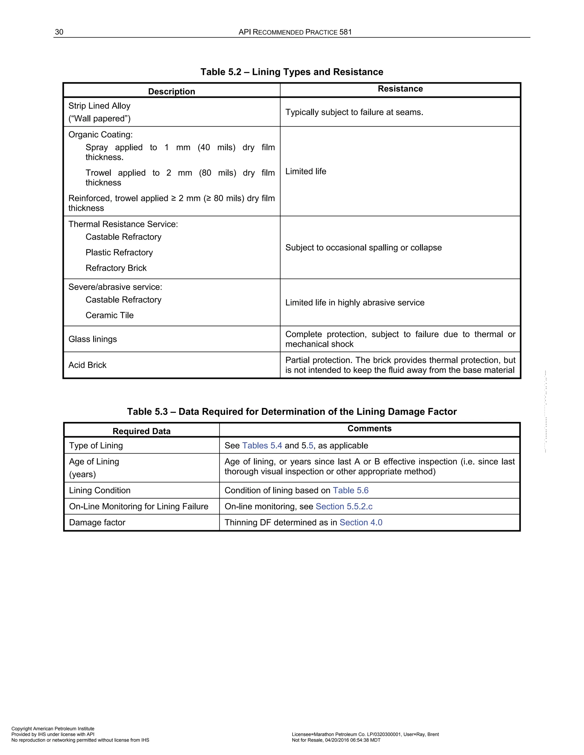
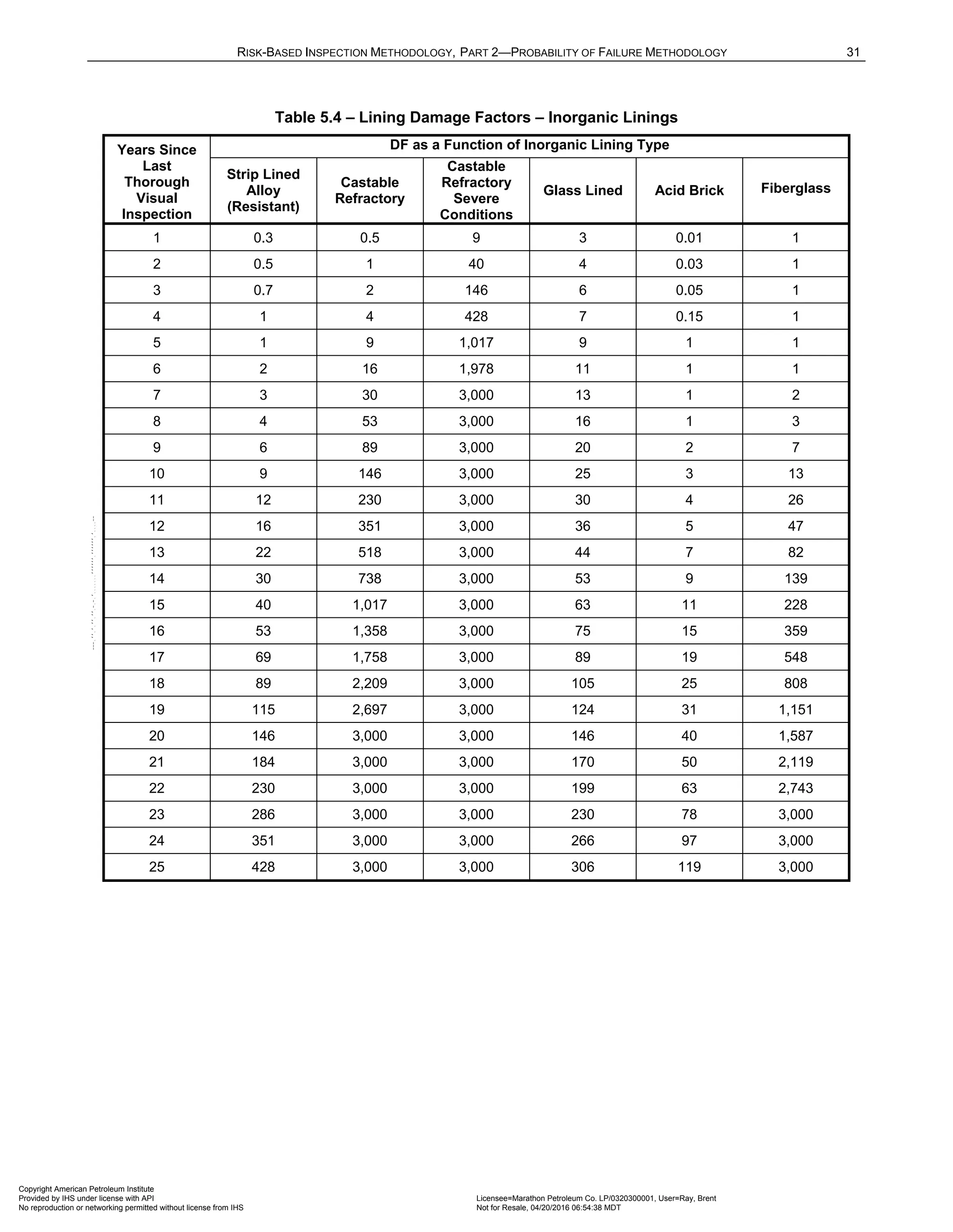
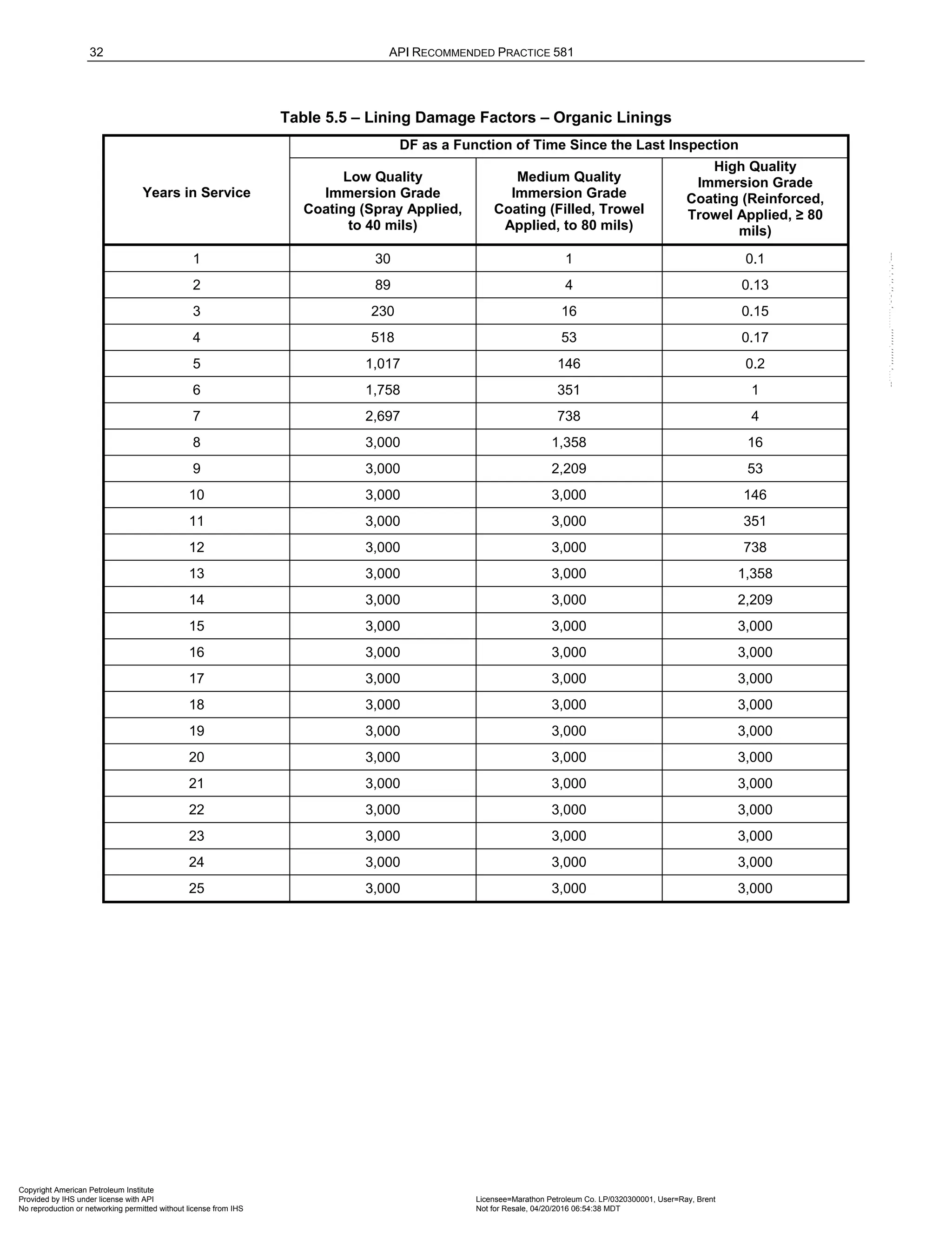
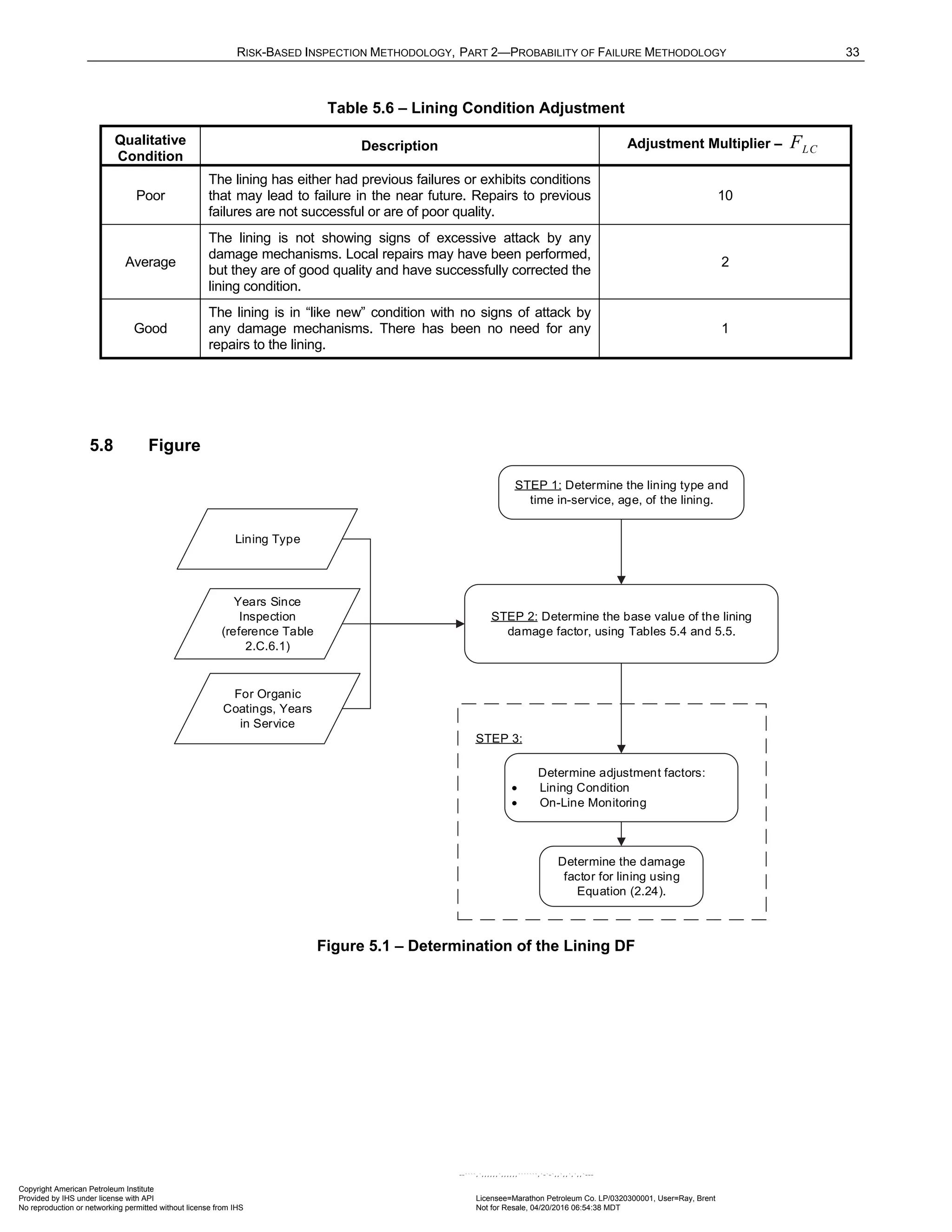
![RISK-BASED INSPECTION METHODOLOGY, PART 2—PROBABILITY OF FAILURE METHODOLOGY 35
Note that a High susceptability should be assigned if cracking was detected during a previous inspection
whether the crack was repaired or left in place based upon FFS evaluation. The High susceptability should be
maintained until subsequent inspections of adequate effectiveness reveal no cracking detected. Cracking
susceptability can then be reassigned by a corrosion specialist.Cracks or arrays of cracks that are found during
an inspection should be evaluated using FFS methods in API 579-1/ASME FFS-1 [10].
6.6 Determination of the Damage Factor
6.6.1 Overview
A flow chart of the steps required to determine the DF for caustic cracking is shown in Figure 6.2. The following
sections provide additional information and the calculation procedure.
6.6.2 Inspection Effectiveness
Inspections are ranked according to their expected effectiveness at detecting caustic cracking.
Examples of inspection activities that are both intrusive (requires entry into the equipment) and non-intrusive
(can be performed externally), are provided in Annex 2.C, Table 2.C.9.3. The number and category of the
highest effective inspection will be used to determine the DF.
If multiple inspections of a lower effectiveness have been conducted during the designated time period, they can
be equated to an equivalent higher effectiveness inspection in accordance with Section 4.4.3.
6.6.3 Calculation of the Damage Factor
The following procedure may be used to determine the DF for caustic cracking, see Figure 6.2.
a) STEP 1 – Determine the susceptibility for cracking using Figure 6.2. Note that a HIGH susceptibility should
be used if cracking is confirmed to be present.
b) STEP 2 – Based on the susceptibility in STEP 1, determine the severity index, VI
S , from Table 6.2.
c) STEP 3 – Determine the time in-service, age , since the last Level A, B or C inspection was performed with
no cracking detected or cracking was repaired. Cracking detected but not repaired should be evaluated and
future inspection recommendations based upon FFS evaluation.
d) STEP 4 – Determine the number of inspections, and the corresponding inspection effectiveness category
using Section 6.6.2 for past inspections performed during the in-service time. Combine the inspections to
the highest effectiveness performed using Section 3.4.3.
e) STEP 5 – Determine the base DF for caustic cracking,
caustic
fB
D , using Table 6.3 based on the number of,
and the highest inspection effectiveness determined in STEP 4, and the severity index, VI
S , from STEP 2.
f) STEP 6 – Calculate the escalation in the DF based on the time in-service since the last inspection using
the age from STEP 3 and Equation (2.25). In this equation, it is assumed that the probability for cracking
will increase with time since the last inspection as a result of increased exposure to upset conditions and
other non-normal conditions.
( )
1.1
[ ,1.0]
caustic caustic
f fB
D D Max age
= ⋅ (2.25)
6.7 Nomenclature
age is the component in-service time since the last cracking inspection or service start date
caustic
f
DF is the DF for caustic cracking
caustic
fB
DF is the base value of the DF for caustic cracking
VI
S is the severity index
Copyright American Petroleum Institute
Provided by IHS under license with API Licensee=Marathon Petroleum Co. LP/0320300001, User=Ray, Brent
Not for Resale, 04/20/2016 06:54:38 MDT
No reproduction or networking permitted without license from IHS
--````,`,,,,,,`,,,,,,```````,`-`-`,,`,,`,`,,`---](https://image.slidesharecdn.com/api581-3rdedition-april2016-240227010601-3bf73ab5/75/Norma-API-581-3rd-Edition-April-2016-pdf-168-2048.jpg)
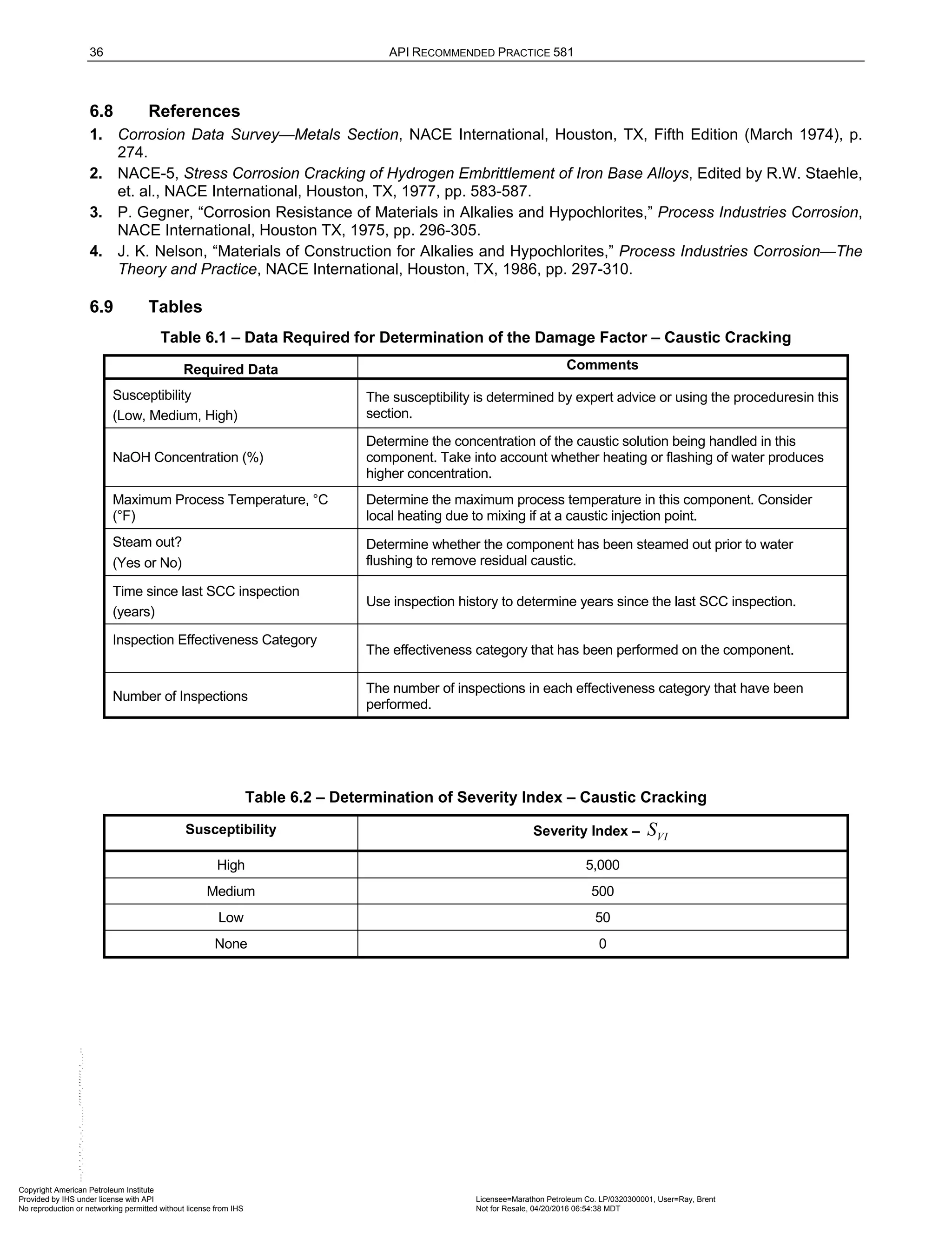
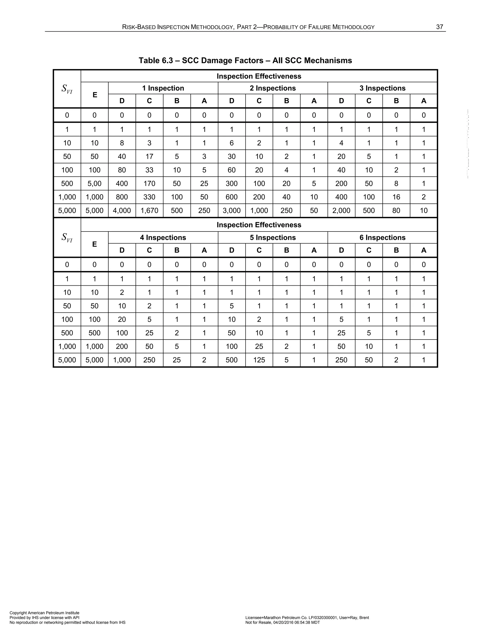
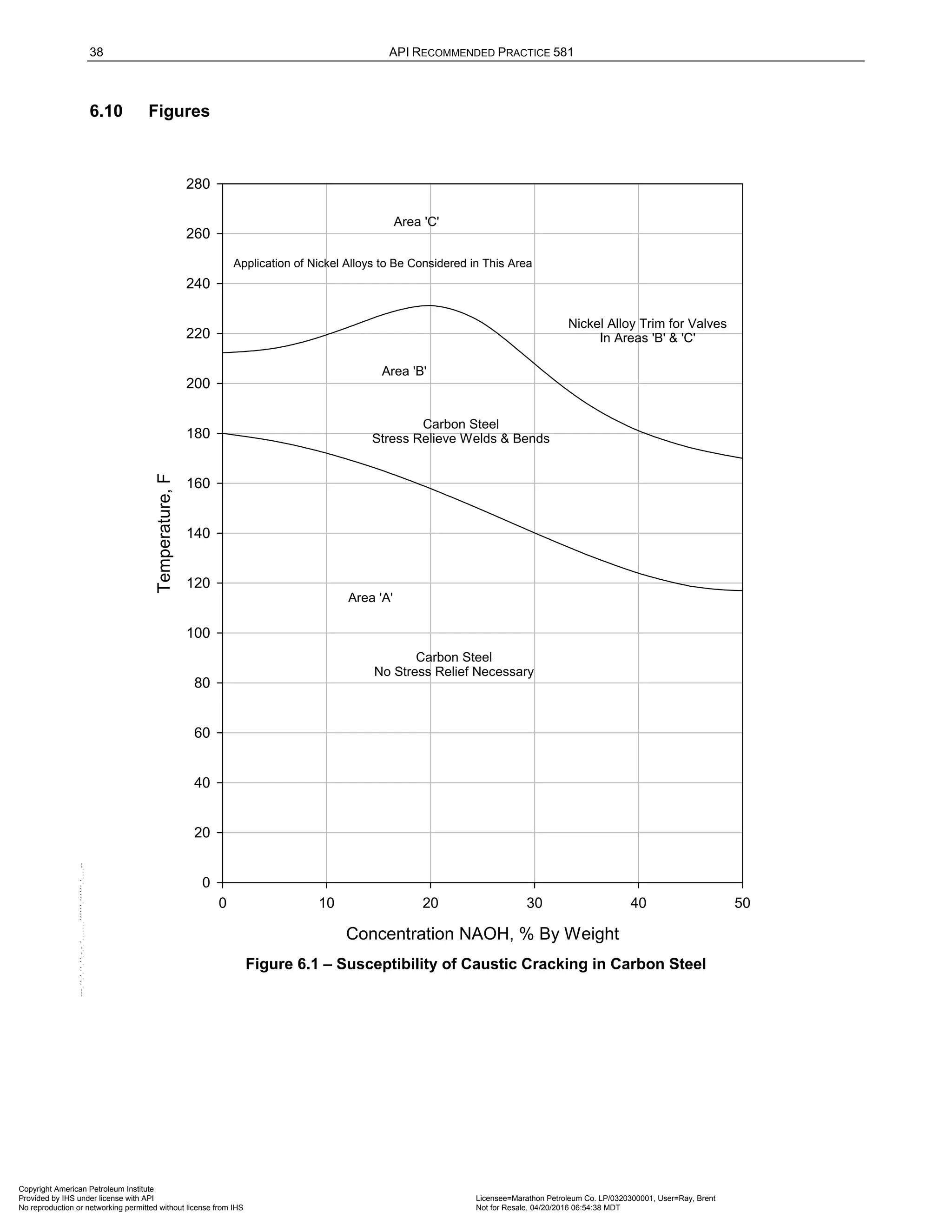
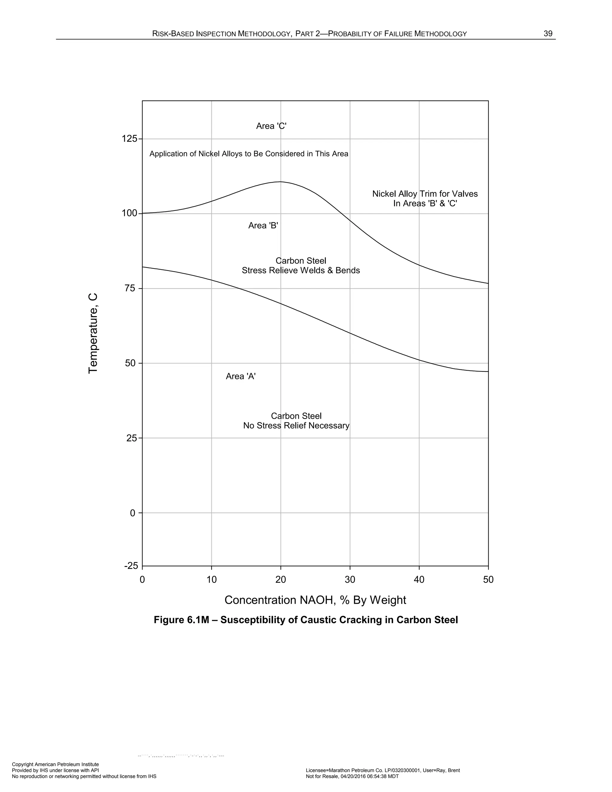
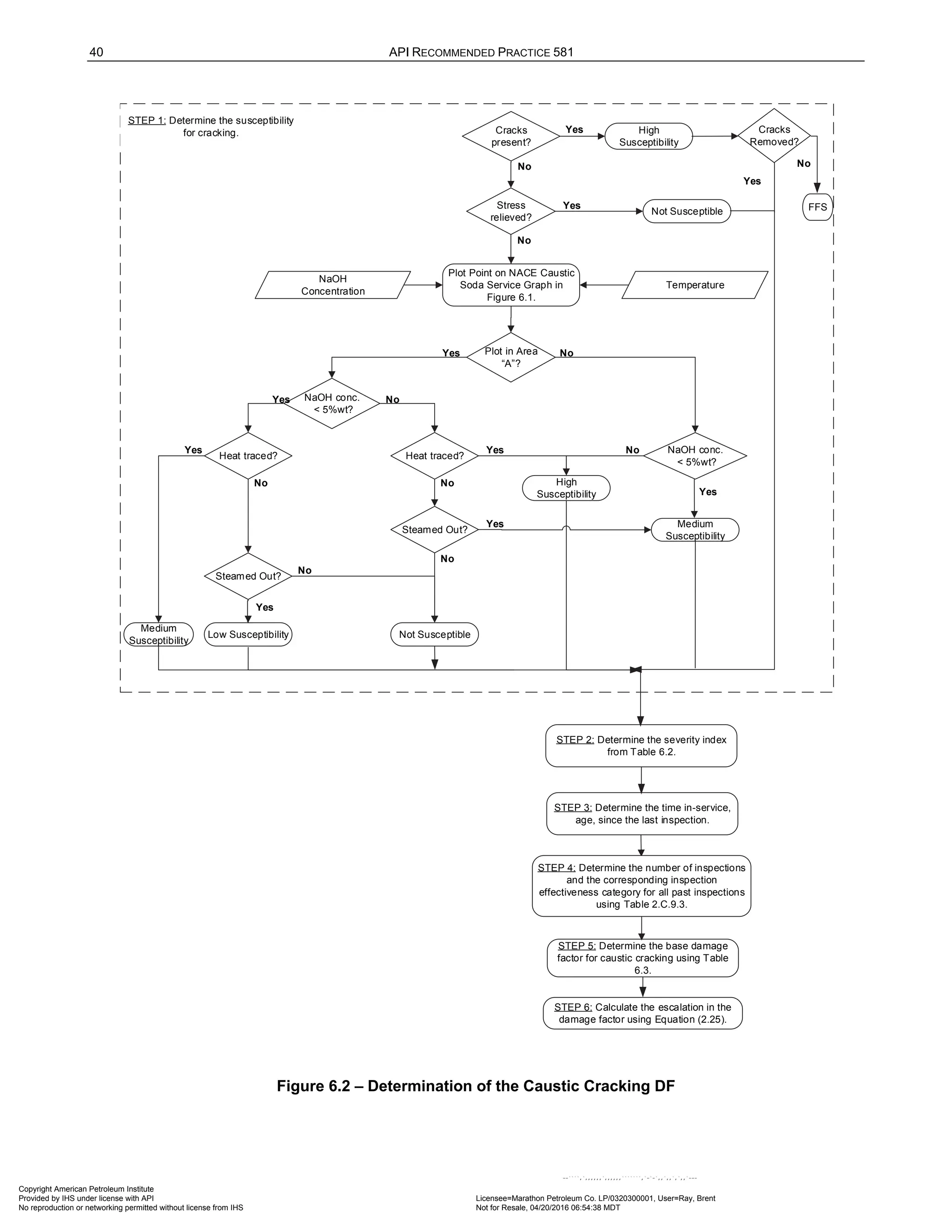
![42 API RECOMMENDED PRACTICE 581
7.4 Required Data
The basic component data required for analysis is given in Table 4.1 and the specific data required for
determination of the amine cracking DF is provided in Table 7.1.
7.5 Basic Assumptions
The main assumption in determining the DF for amine cracking is that the damage can be characterized by a
susceptibility parameter that is designated as high, medium, or low based on process environment, material of
construction, and component fabrication variables (i.e. heat treatment). Based on the susceptibility parameter, a
Severity Index is assigned that is a measure of the component susceptibility to cracking (or the probability of
initiating cracks) and the probability that the crack will result in a leak.
If cracking is detected in the component during an inspection, the susceptibility is designated as High, and this
will result in the maximum value for the Severity Index. Cracks or arrays of cracks that are found during an
inspection should be evaluated using Fitness-For-Service methods in API 579-1/ASME FFS-1 [10].
7.6 Determination of the Damage Factor
7.6.1 Overview
A flow chart of the steps required to determine the DF for amine cracking is shown in Figure 7.1. The following
sections provide additional information and the calculation procedure.
7.6.2 Inspection Effectiveness
Inspections are ranked according to their expected effectiveness at detecting amine cracking. Examples of
inspection activities that are both intrusive (requires entry into the equipment) and non-intrusive (can be
performed externally), are provided in Annex 2.C, Table 2.C.9.1.
If multiple inspections of a lower effectiveness have been conducted during the designated time period, they can
be equated to an equivalent higher effectiveness inspection in accordance with Section 4.4.3.
7.6.3 Calculation of the Damage Factor
The following procedure may be used to determine the DF for amine cracking, see Figure 7.1.
a) STEP 1 – Determine the susceptibility for cracking using Figure 7.1. Note that a HIGH susceptibility should
be used if cracking is confirmed to be present.
b) STEP 2 – Based on the susceptibility in STEP 3, determine the severity index, VI
S , from Table 7.2.
c) STEP 3 – Determine the time in-service, age , since the last Level A, B or C inspection was performed
with no cracking detected or cracking was repaired. Cracking detected but not repaired should be
evaluated and future inspection recommendations based upon FFS evaluation.
d) STEP 4 – Determine the number of inspections, and the corresponding inspection effectiveness category
using Section 7.6.2 for past inspections performed during the in-service time. Combine the inspections to
the highest effectiveness performed using Section 3.4.3.
e) STEP 5 – Determine the base DF for amine cracking,
amine
fB
D , using Table 6.3 based on the number of, and
the highest inspection effectiveness determined in STEP 4, and the severity index, VI
S , from STEP 2.
f) STEP 6 – Calculate the escalation in the DF based on the time in-service since the last inspection using
the age from STEP 3 and Equation (2.26). In this equation, it is assumed that the probability for cracking
will increase with time since the last inspection as a result of increased exposure to upset conditions and
other non-normal conditions.
( )
1.1
[ ,1.0]
amine amine
f fB
D D Max age
= ⋅ (2.26)
Copyright American Petroleum Institute
Provided by IHS under license with API Licensee=Marathon Petroleum Co. LP/0320300001, User=Ray, Brent
Not for Resale, 04/20/2016 06:54:38 MDT
No reproduction or networking permitted without license from IHS
--````,`,,,,,,`,,,,,,```````,`-`-`,,`,,`,`,,`---](https://image.slidesharecdn.com/api581-3rdedition-april2016-240227010601-3bf73ab5/75/Norma-API-581-3rd-Edition-April-2016-pdf-175-2048.jpg)
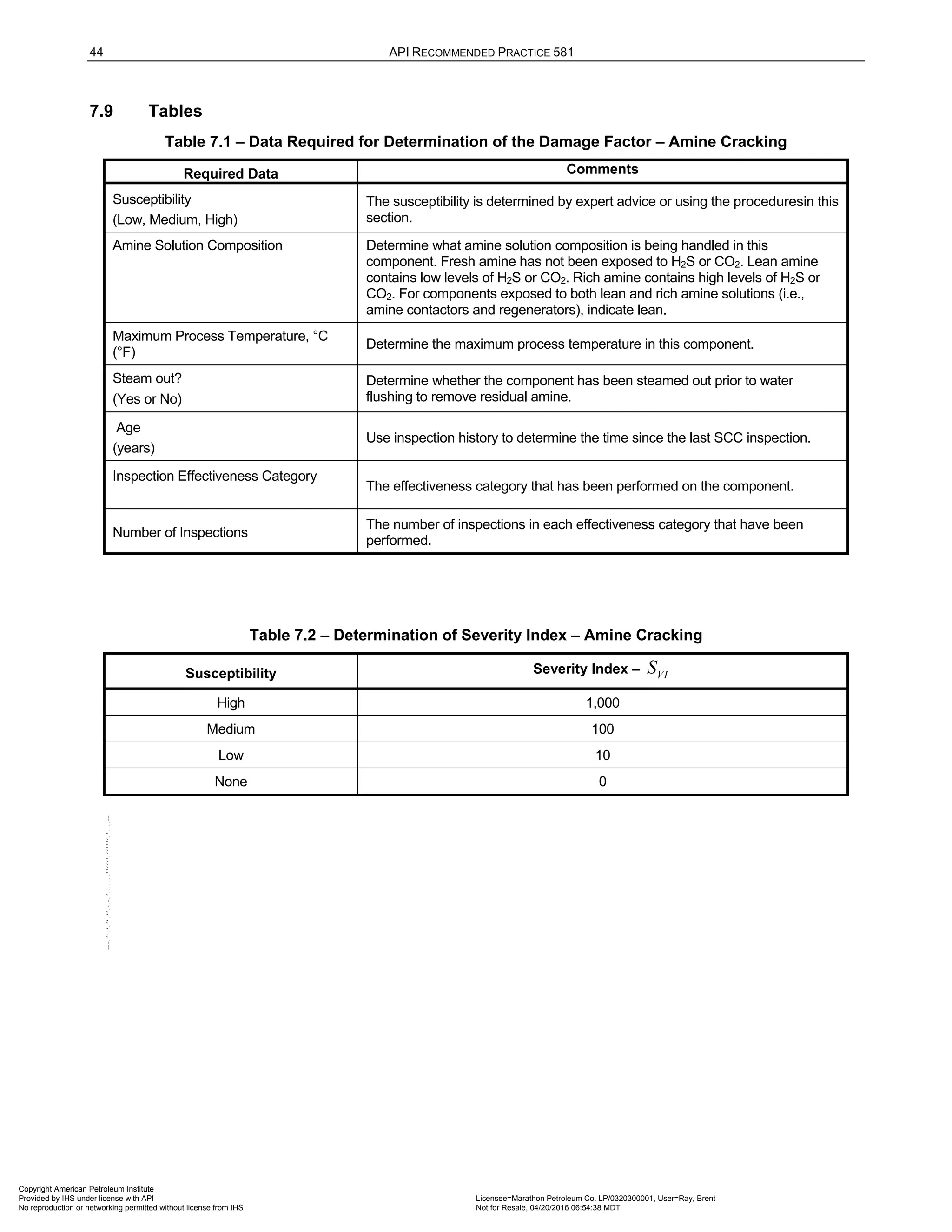
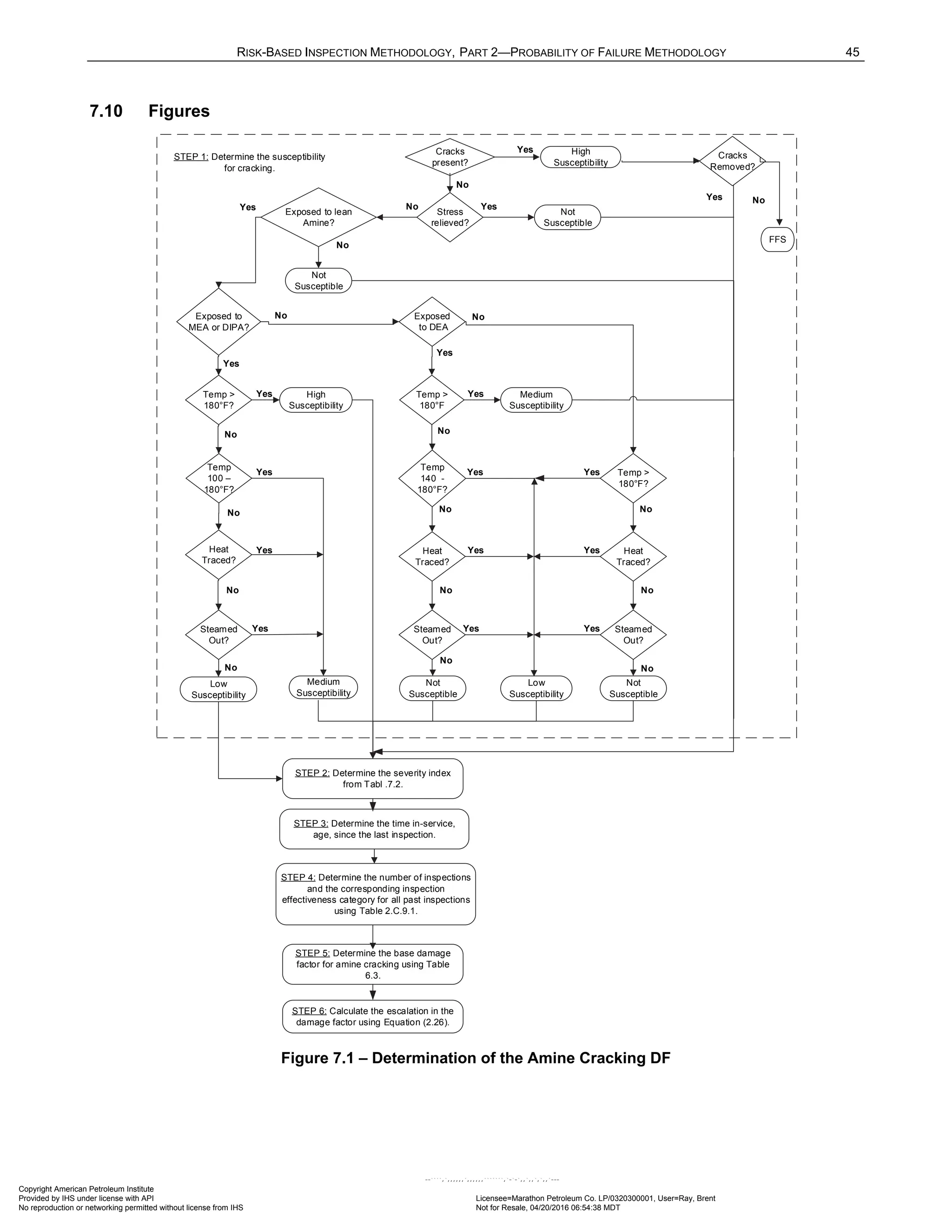
![46 API RECOMMENDED PRACTICE 581
8 Scc Damage Factor – Sulfide Stress Cracking
8.1 Scope
The DF calculation for components subject to Sulfide Stress Cracking (SSC) is covered in this section.
8.2 Description of Damage
SSC is defined as cracking of a metal under the combined action of tensile stress and corrosion in the presence
of water and hydrogen sulfide. SSC is a form of hydrogen stress cracking resulting from absorption of atomic
hydrogen that is produced by the sulfide corrosion process on the metal surface. SSC usually occurs more
readily in high strength (high hardness) steels in hard weld deposits or hard heat-affected zones (HAZs) of
lower-strength steels. Susceptibility to SSC is related to the hydrogen permeation flux in the steel, which is
primarily associated with two environmental parameters, pH and H2S content of the water. Typically, the
hydrogen flux in steels has been found to be lowest in near neutral pH solutions, with increasing flux at both
lower and higher pH values. Corrosion at low pH values is caused by H2S, whereas corrosion at high pH values
is caused by high concentrations of the bisulfide ion. Presence of cyanides at elevated pH can further aggravate
the hydrogen penetration into the steel. SSC susceptibility is known to increase with H2S content, e.g. H2S
partial pressure in the gas phase or H2S content of the water phase. The presence of as little as 1 ppm of H2S in
the water has been found to be sufficient to cause SSC.
Susceptibility to SSC is primarily related to two material parameters, hardness and stress level. High hardness
of the steel increases its susceptibility to SSC. SSC has not generally been a concern for carbon steel base
materials typically used for refinery pressure vessels and piping in wet hydrogen sulfide service because these
steels have sufficiently low strength (hardness) levels. However, weld deposits and HAZs may contain zones of
high hardness and high residual stresses from welding. High residual tensile stresses associated with welds
increases susceptibility to SSC. PWHT significantly reduces residual stresses and also tempers (softens) weld
deposits and HAZs. A post weld heat treatment of about 621°C (1150°F) for one hour per inch of thickness (one
hour minimum) is considered effective for carbon steel. Somewhat higher temperatures are required for low
alloy steels. Control of hardness and reduction of residual stresses are recognized methods for preventing SSC
as outlined in NACE Standard RP0472.
8.3 Screening Criteria
If the component’s material of construction is carbon or low alloy steel and the process environment contains
water and H2S in any concentration, then the component should be evaluated for susceptibility to SSC.
8.4 Required Data
The basic component data required for analysis is given in Table 4.1 and the specific data required for
determination of the sulfide stress cracking DF is provided in Table 8.1.
8.5 Basic Assumptions
The main assumption in determining the DF for SSC is that the damage can be characterized by a susceptibility
parameter that is designated as high, medium, or low based on process environment, material of construction,
and component fabrication variables (i.e. heat treatment). Based on the susceptibility parameter, a Severity
Index is assigned that is a measure of the component susceptibility to cracking (or the probability of initiating
cracks) and the probability that the crack will result in a loss of containment.
If cracking is detected in the component during an inspection, the susceptibility is designated as High, and this
will result in the maximum value for the Severity Index. Cracks or arrays of cracks that are found during an
inspection should be evaluated using Fitness-For-Service methods in API 579-1/ASME FFS-1 [10].
8.6 Determination of the Damage Factor
8.6.1 Overview
A flow chart of the steps required to determine the DF for SSC is shown in Figure 8.1. The following sections
provide additional information and the calculation procedure.
Copyright American Petroleum Institute
Provided by IHS under license with API Licensee=Marathon Petroleum Co. LP/0320300001, User=Ray, Brent
Not for Resale, 04/20/2016 06:54:38 MDT
No reproduction or networking permitted without license from IHS
--````,`,,,,,,`,,,,,,```````,`-`-`,,`,,`,`,,`---](https://image.slidesharecdn.com/api581-3rdedition-april2016-240227010601-3bf73ab5/75/Norma-API-581-3rd-Edition-April-2016-pdf-179-2048.jpg)
![RISK-BASED INSPECTION METHODOLOGY, PART 2—PROBABILITY OF FAILURE METHODOLOGY 47
8.6.2 Inspection Effectiveness
Inspections are ranked according to their expected effectiveness at detecting SSC. Examples of inspection
activities that are both intrusive (requires entry into the equipment) and non-intrusive (can be performed
externally), are provided in Annex 2.C, Table 2.C.9.6.
If multiple inspections of a lower effectiveness have been conducted during the designated time period, they can
be equated to an equivalent higher effectiveness inspection in accordance with Section 3.4.3.
8.6.3 Calculation of the Damage Factor
The following procedure may be used to determine the DF for sulfide stress cracking, see Figure 8.1.
a) STEP 1 – Determine the environmental severity (potential level of hydrogen flux) for cracking based on the
H2S content of the water and its pH using Table 8.2.
b) STEP 2 – Determine the susceptibility for cracking using Figure 8.1 and Table 8.3 based on the
environmental severity from STEP 1, the maximum Brinnell hardness of weldments, and knowledge of
whether the component was subject to PWHT. Note that a HIGH susceptibility should be used if cracking is
confirmed to be present.
c) STEP 3 – Based on the susceptibility in STEP 3, determine the severity index, VI
S , from Table 8.4.
d) STEP 4 – Determine the time in-service, age , since the last Level A, B or C inspection was performed
with no cracking detected or cracking was repaired. Cracking detected but not repaired should be
evaluated and future inspection recommendations based upon FFS evaluation.
e) STEP 5 – Determine the number of inspections, and the corresponding inspection effectiveness category
using Section 8.6.2 for past inspections performed during the in-service time. Combine the inspections to
the highest effectiveness performed using Section 3.4.3.
f) STEP 6 – Determine the base DF for sulfide stress cracking,
ssc
fB
D , using Table 6.3 based on the number
of, and the highest inspection effectiveness determined in STEP 5, and the severity index, VI
S , from STEP
3.
g) STEP 7 – Calculate the escalation in the DF based on the time in-service since the last inspection using
the age from STEP 4 and Equation (2.27). In this equation, it is assumed that the probability for cracking
will increase with time since the last inspection as a result of increased exposure to upset conditions and
other non-normal conditions.
( )
1.1
[ ,1.0]
ssc ssc
f fB
D D Max age
= ⋅ (2.27)
8.7 Nomenclature
age is the component in-service time since the last cracking inspection or service start date
ssc
f
D is the DF for sulfide stress cracking
ssc
fB
D is the base value of the DF for SSC
VI
S is the severity index
Copyright American Petroleum Institute
Provided by IHS under license with API Licensee=Marathon Petroleum Co. LP/0320300001, User=Ray, Brent
Not for Resale, 04/20/2016 06:54:38 MDT
No reproduction or networking permitted without license from IHS
--````,`,,,,,,`,,,,,,```````,`-`-`,,`,,`,`,,`---](https://image.slidesharecdn.com/api581-3rdedition-april2016-240227010601-3bf73ab5/75/Norma-API-581-3rd-Edition-April-2016-pdf-180-2048.jpg)
![48 API RECOMMENDED PRACTICE 581
8.8 References
1. NACE RP0472, Methods and Controls to Prevent In-Service Cracking of Carbon Steel Welds in Corrosive
Petroleum Refining Environments, NACE International, Houston, TX.
2. R. R. Petrie and E. M. Moore, Jr., “Determining the Suitability of Existing Pipelines and Producing Facilities
for Wet Sour Service,” Materials Performance 28, 6 (June 1989), pp. 59-65.
3. NACE Publication 8X294, Review of Published Literature on Wet H2S Cracking of Steels Through 1989
4. Stress Corrosion Cracking and Hydrogen Embrittlement of Iron Base Alloys, NACE-5, Edited by R. W.
Staehle, et. al., NACE International, Houston, TX, 1977, pp. 541-559.
5. C. M. Hudgins, et. al., “Hydrogen Sulfide Cracking of Carbon and Alloy Steels,” Corrosion, Vol. 22, pp. 238-
251.
6. NACE RP0296-96, Guidelines for Detection, Repair, and Mitigation of Existing Petroleum Refinery
Pressure Vessels in Wet H2S Environments, NACE International, Houston, TX.
8.9 Tables
Table 8.1 – Data Required for Determination of the Damage Factor – SSC
Required Data Comments
Susceptibility
(Low, Medium, High)
The susceptibility is determined by expert advice or using the proceduresin this
section.
Presence of Water
(Yes or No)
Determine whether free water is present in the component. Consider not
only normal operating conditions, but also startup, shutdown, process
upsets, etc.
H2S Content of Water Determine the H2S content of the water phase. If analytical results are not
readily available, it can be estimated using the approach of Petrie & Moore
[17].
pH of Water Determine the pH of the water phase. If analytical results are not readily
available, it should be estimated by a knowledgeable process engineer.
Presence of Cyanides
(Yes or No)
Determine the presence of cyanide through sampling and/or field analysis.
Consider primarily normal and upset operations but also startup and
shutdown conditions.
Max Brinnell Hardness Determine the maximum Brinnell hardness actually measured at the
weldments of the steel components. Report readings actually taken as
Brinnell, not converted from finer techniques (e.g., Vickers, Knoop, etc.) If
actual readings are not available, use the maximum allowable hardness
permitted by the fabrication specification.
Age
(years)
Use inspection history to determine the time since the last SCC inspection.
Inspection Effectiveness Category
The effectiveness category that has been performed on the component.
Number of Inspections
The number of inspections in each effectiveness category that have been
performed.
Copyright American Petroleum Institute
Provided by IHS under license with API Licensee=Marathon Petroleum Co. LP/0320300001, User=Ray, Brent
Not for Resale, 04/20/2016 06:54:38 MDT
No reproduction or networking permitted without license from IHS
--````,`,,,,,,`,,,,,,```````,`-`-`,,`,,`,`,,`---](https://image.slidesharecdn.com/api581-3rdedition-april2016-240227010601-3bf73ab5/75/Norma-API-581-3rd-Edition-April-2016-pdf-181-2048.jpg)
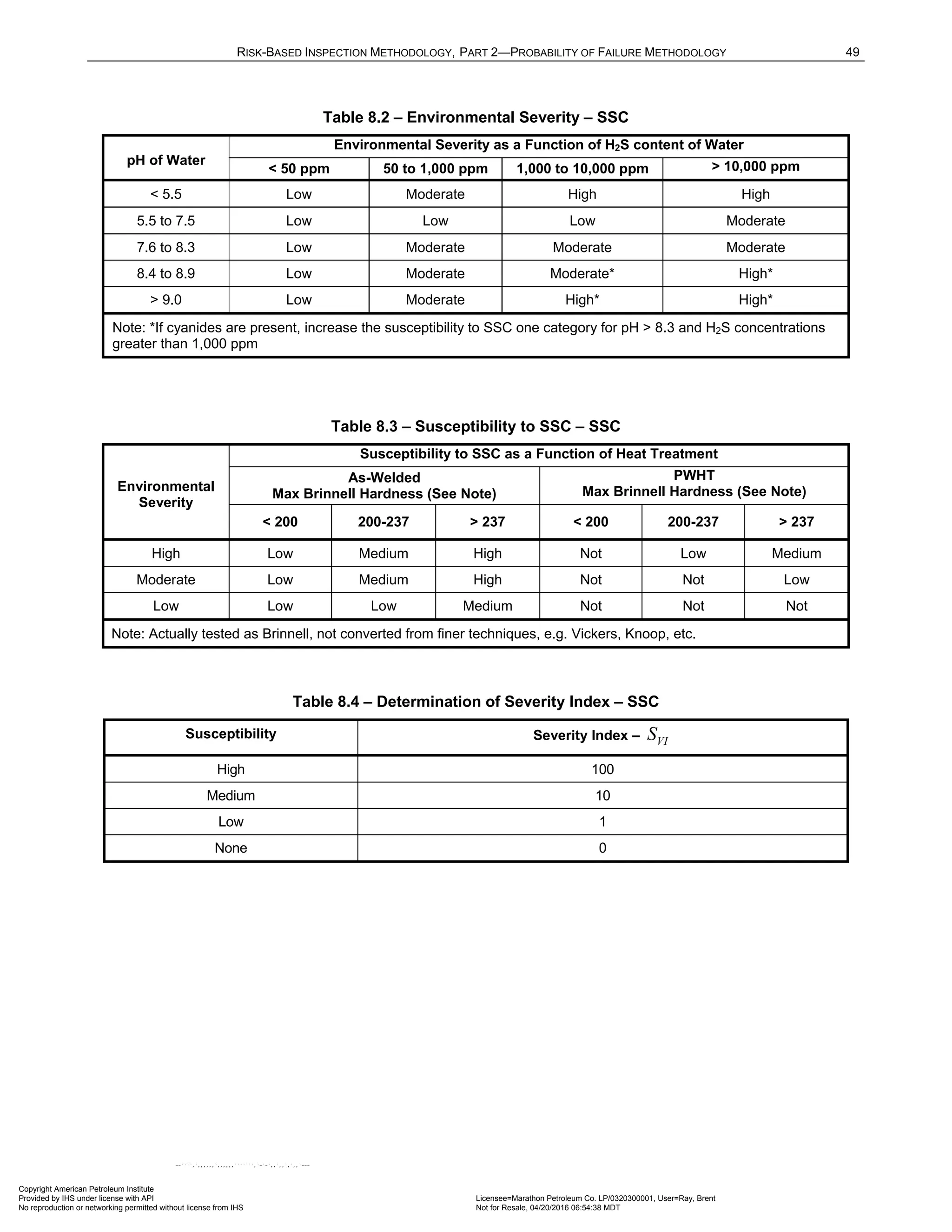
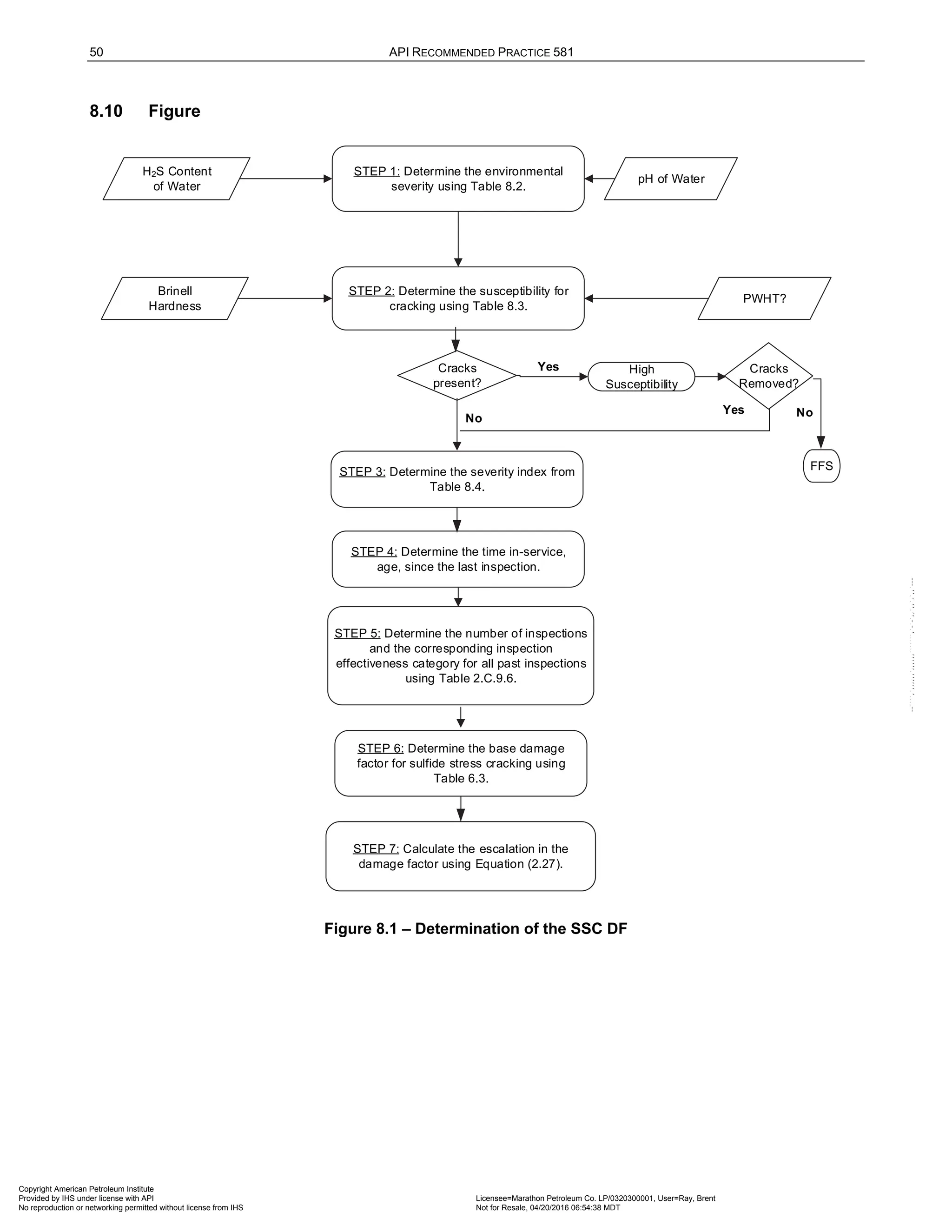
![52 API RECOMMENDED PRACTICE 581
9.5 Basic Assumptions
The main assumption in determining the DF for HIC/SOHIC-H2S cracking is that the damage can be
characterized by a susceptibility parameter that is designated as high, medium, or low based on process
environment, material of construction, and component fabrication variables (i.e. heat treatment). Based on the
susceptibility parameter, a Severity Index is assigned that is a measure of the component susceptibility to
cracking (or the probability of initiating cracks) and the probability that the crack will result in a leak.
If SOHIC is detected in the component during an inspection, the susceptibility is designated as High, and this
will result in the maximum value for the Severity Index. Known blisters or cracks that are found during an
inspection should be evaluated using Fitness-For-Service methods in API 579-1/ASME FFS-1 [10].
9.6 Determination of the Damage Factor
9.6.1 Overview
A flow chart of the steps required to determine the DF for HIC/SOHIC-H2S cracking is shown in Figure 9.1. The
following sections provide additional information and the calculation procedure.
9.6.2 Inspection Effectiveness
Inspections are ranked according to their expected effectiveness at detecting for HIC/SOHIC-H2S. Examples of
inspection activities that are both intrusive (requires entry into the equipment) and non-intrusive (can be
performed externally), are provided in Annex 2.C, Table 2.C.9.9.
If multiple inspections of a lower effectiveness have been conducted during the designated time period, they can
be equated to an equivalent higher effectiveness inspection in accordance with Section 3.4.3.
9.6.3 Adjustment for On-Line Monitoring
In addition to inspection, on-line monitoring using hydrogen probes and/or key process variables provides a
better understanding of HIC/SOHIC-H2S susceptibility. The advantage of on-line monitoring is that process
changes affecting SCC susceptibility can be detected before significant cracking occurs. This earlier detection
could permit more timely action to decrease the POF. For HIC/SOHIC-H2S, an on-line monitoring factor of 2 is
applied if either hydrogen probes or monitoring of key process variables are used. If both hydrogen probes and
monitoring of key process variables are used, an on-line monitoring factor is 4 is applied.
9.6.4 Calculation of the Damage Factor
The following procedure may be used to determine the DF for HIC/SOHIC-H2S cracking, see Figure 9.1.
a) STEP 1 – Determine the environmental severity (potential level of hydrogen flux) for cracking based on the
H2S content of the water and its pH using Table 9.2. Note that a HIGH environmental severity should be
used if cracking is confirmed to be present.
b) STEP 2 – Determine the susceptibility for cracking using Figure 9.1 and Table 9.3 based on the
environmental severity from STEP 1, the sulfur content of the carbon steel, product form and knowledge of
whether the component was subject to PWHT.
c) STEP 3 – Based on the susceptibility in STEP 2, determine the severity index, VI
S , from Table 9.4.
d) STEP 4 – Determine the time in-service, age , since the last Level A, B or C inspection was performed
performed with no cracking detected or cracking was repaired. Cracking detected but not repaired should
be evaluated and future inspection recommendations based upon FFS evaluation.
e) STEP 5 – Determine the number of inspections, and the corresponding inspection effectiveness category
using Section 9.6.2 for past inspections performed during the in-service time. Combine the inspections to
the highest effectiveness performed using Section 3.4.3.
f) STEP 6 – Determine the base DF for HIC/SOHIC-H2S cracking,
2
/
HIC SOHIC H S
fB
D −
, using Table 6.3 based on
the number of, and the highest inspection effectiveness determined in STEP 5, and the severity index, VI
S ,
from STEP 3.
Copyright American Petroleum Institute
Provided by IHS under license with API Licensee=Marathon Petroleum Co. LP/0320300001, User=Ray, Brent
Not for Resale, 04/20/2016 06:54:38 MDT
No reproduction or networking permitted without license from IHS
--````,`,,,,,,`,,,,,,```````,`-`-`,,`,,`,`,,`---](https://image.slidesharecdn.com/api581-3rdedition-april2016-240227010601-3bf73ab5/75/Norma-API-581-3rd-Edition-April-2016-pdf-185-2048.jpg)
![RISK-BASED INSPECTION METHODOLOGY, PART 2—PROBABILITY OF FAILURE METHODOLOGY 53
g) STEP 7 – Determine the on-line adjustment factor, OM
F , from Table 9.5.
h) STEP 8 – Calculate the final DF accounting for escalation based on the time in-service since the last
inspection using the age from STEP 4 and Equation (2.28). In this equation, it is assumed that the
probability for cracking will increase with time since the last inspection as a result of increased exposure to
upset conditions and other non-normal conditions. The equation also applies the adjustment factor for on-
line monitoring.
( )
2
2
1.1
/
/ [ ,1.0]
HIC SOHIC H S
fB
HIC SOHIC H S
f
OM
D Max age
D
F
−
− ⋅
= (2.28)
9.7 Nomenclature
age is the component in-service time since the last cracking inspection or service start date
2
/
HIC SOHIC H S
f
D −
is the DF for HIC/SOHIC-H2S cracking
2
/
HIC SOHIC H S
fB
D −
is the base value of the for HIC/SOHIC-H2S cracking
OM
F is the on-line monitoring adjustment factor
VI
S is the severity index
9.8 References
1. R. R. Petrie and E. M. Moore, Jr., “Determining the Suitability of Existing Pipelines and Producing Facilities
for Wet Sour Service,” Materials Performance 28, 6 (June 1989), pp. 59-65.
2. R. D. Merrick, “Refinery Experiences with Cracking in Wet H2S Environments,” Materials Performance 27, 1
(January 1988), pp. 30.
3. R. D. Merrick and M.L. Bullen, “Prevention of Cracking in Wet H2S Environments,” NACE Corrosion/89,
paper no. 269.
4. NACE Publication 8X194, Materials and Fabrication Practices for New Pressure Vessels Used in Wet H2S
Refinery Service, NACE International, Houston, TX.
5. NACE Publication 8X294, Review of Published Literature on Wet H2S Cracking of Steels Through 1989,
NACE International, Houston, TX.
6. API Publication 939, Research Report on Characterization and Monitoring of Cracking in Wet H2S Service,
American Petroleum Institute, Washington, D.C., 20005, October 1994.
7. M. S. Cayard and R. D. Kane, “Characterization and Monitoring of Cracking of Steel Equipment in Wet H2S
Service,” NACE Corrosion/95, Paper no. 329.
8. NACE RP0296-96, Guidelines for Detection, Repair, and Mitigation of Existing Petroleum Refinery Pressure
Vessels in Wet H2S Environments, NACE International, Houston, TX.
Copyright American Petroleum Institute
Provided by IHS under license with API Licensee=Marathon Petroleum Co. LP/0320300001, User=Ray, Brent
Not for Resale, 04/20/2016 06:54:38 MDT
No reproduction or networking permitted without license from IHS
--````,`,,,,,,`,,,,,,```````,`-`-`,,`,,`,`,,`---](https://image.slidesharecdn.com/api581-3rdedition-april2016-240227010601-3bf73ab5/75/Norma-API-581-3rd-Edition-April-2016-pdf-186-2048.jpg)
![54 API RECOMMENDED PRACTICE 581
9.9 Tables
Table 9.1 – Data Required for Determination of the Damage Factor – HIC/SOHIC-H2S Cracking
Required Data Comments
Susceptibility
(Low, Medium, High)
The susceptibility is determined by expert advice or using the proceduresin
this section.
Presence of Water
(Yes or No)
Determine whether free water is present in the component. Consider not
only normal operating conditions, but also startup, shutdown, process
upsets, etc.
H2S Content of Water Determine the H2S content of the water phase. If analytical results are not
readily available, it can be estimated using the approach of Petrie & Moore
[22].
pH of Water Determine the pH of the water phase. If analytical results are not readily
available, it should be estimated by a knowledgeable process engineer.
Presence of Cyanides
(Yes or No)
Determine the presence of cyanide through sampling and/or field analysis.
Consider primarily normal and upset operations but also startup and
shutdown conditions.
Sulfur Content of Plate Steel Determine the sulfur content of the steel used to fabricate the component.
This information should be available on MTR’s in equipment files. If not
available, it can be estimated from the ASTM or ASME specification of the
steel listed on the U-1 form in consultation with materials engineer.
Steel Product Form
(Plate or Pipe)
Determine what product form of steel was used to fabricate the component.
Most components are fabricated from rolled and welded steel plates (e.g.
A285, A515, A516,, etc.), but some small-diameter components is fabricated
from steel pipe and piping components. Most small-diameter piping is
fabricated from steel pipe (e.g. A106, A53, API 5L, etc.) and piping
components (e.g. A105, A234, etc.), but most large diameter piping (above
approximately NPS 16 diameter) is fabricated from rolled and welded plate
steel.
Age
(years)
Use inspection history to determine the time since the last SCC inspection.
Inspection Effectiveness Category
The effectiveness category that has been performed on the component.
On-Line Monitoring
(Hydrogen Probes, Process Variables
or Combination)
The type of proactive corrosion monitoring methods or tools employed such as
hydrogen probes and/or process variable monitoring.
Number of Inspections
The number of inspections in each effectiveness category that have been
performed.
Copyright American Petroleum Institute
Provided by IHS under license with API Licensee=Marathon Petroleum Co. LP/0320300001, User=Ray, Brent
Not for Resale, 04/20/2016 06:54:38 MDT
No reproduction or networking permitted without license from IHS
--````,`,,,,,,`,,,,,,```````,`-`-`,,`,,`,`,,`---](https://image.slidesharecdn.com/api581-3rdedition-april2016-240227010601-3bf73ab5/75/Norma-API-581-3rd-Edition-April-2016-pdf-187-2048.jpg)
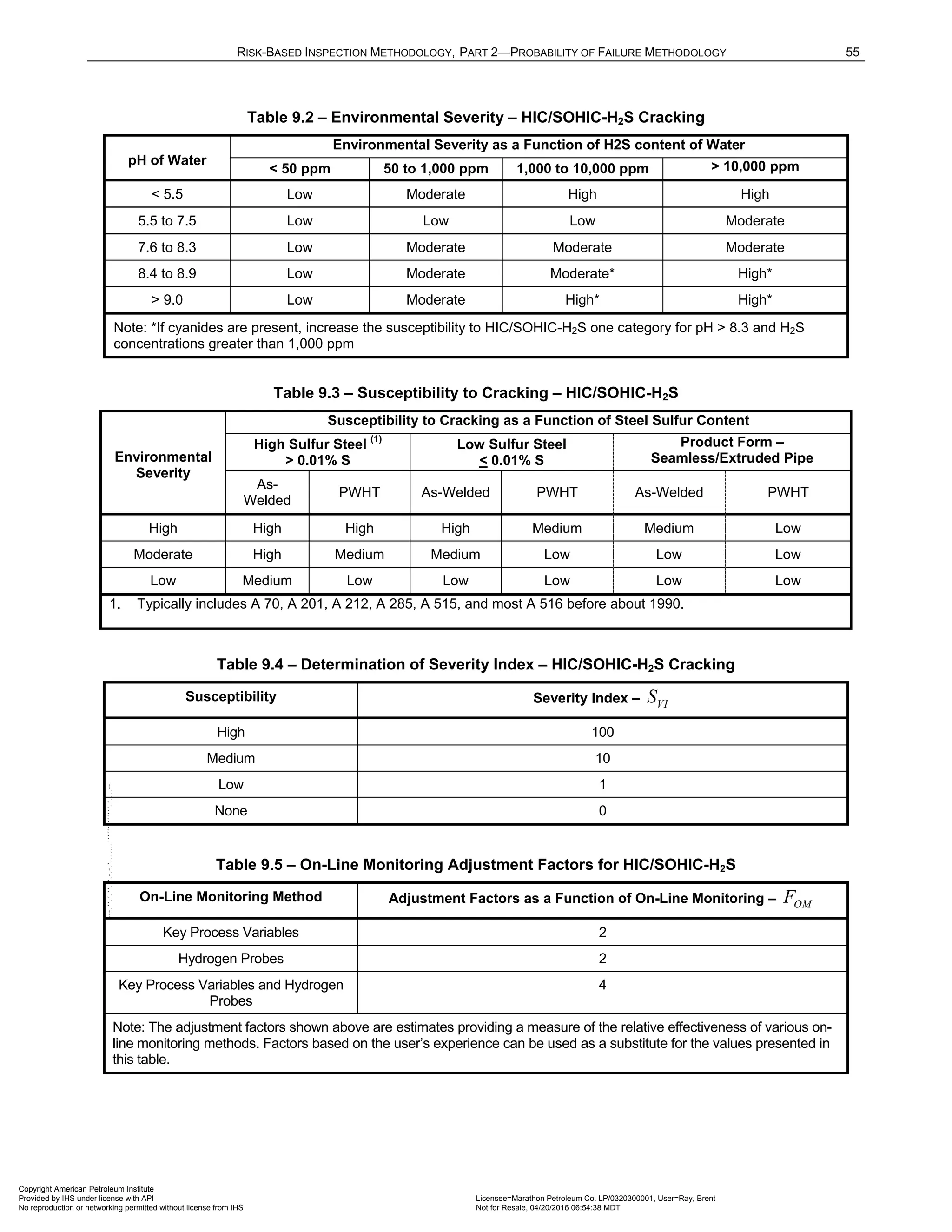
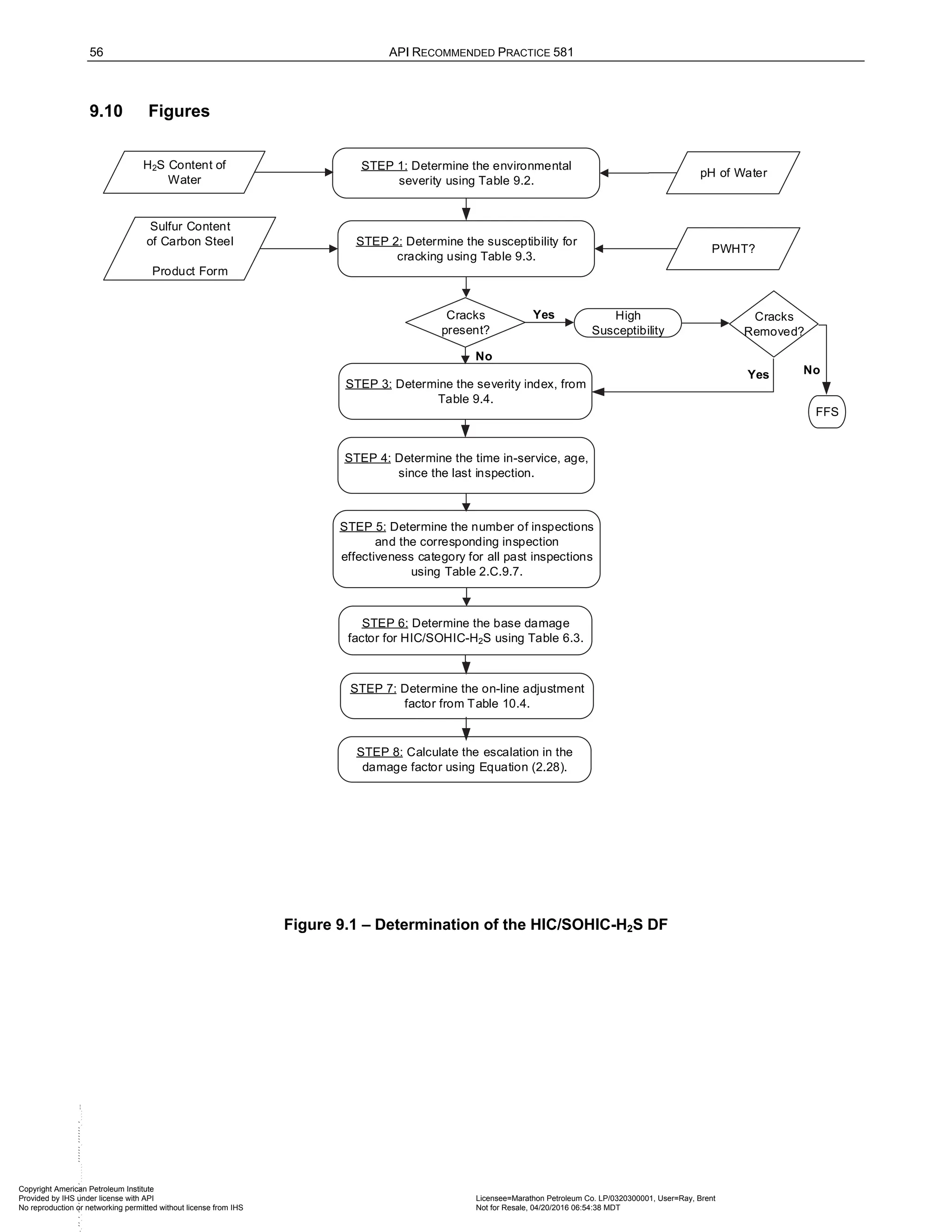

![58 API RECOMMENDED PRACTICE 581
10.3 Screening Criteria
If the component’s material of construction of the component is carbon or low alloy steel and the process
environment contains alkaline water at pH > 7.5 in any concentration, then the component should be considered
for evaluation for susceptibility to ACSCC. Another trigger would be changes in FCCU feed sulfur and nitrogen
contents particularly when feed changes have reduced sulfur (low sulfur feeds or hydroprocessed feeds) or
increased nitrogen [7].
10.4 Required Data
The basic component data required for analysis is given in Table 4.1 and the specific data required for
determination of the ACSCC DF is provided in Table 11.1.
10.5 Basic Assumptions
The main assumption in determining the DF for ACSCC is that the damage can be characterized by a
susceptibility parameter that is designated as high, medium, or low based on process environment, material of
construction, and component fabrication variables (i.e. heat treatment). Based on the susceptibility parameter, a
Severity Index is assigned that is a measure of the component susceptibility to cracking (or the probability of
initiating cracks) and the probability that the crack will result in a leak.
If cracks are detected in the component during an inspection, the susceptibility is designated as High, and this
will result in the maximum value for the Severity Index. Cracks that are found during an inspection should be
evaluated using Fitness-For-Service methods in API 579-1/ASME FFS-1 [10].
10.6 Determination of the Damage Factor
10.6.1 Overview
A flow chart of the steps required to determine the DF for ACSCC is shown in Figure 10.1. The following
sections provide additional information and the calculation procedure.
10.6.2 Inspection Effectiveness
Inspections are ranked according to their expected effectiveness at detecting for ACSCC. Examples of
inspection activities that are both intrusive (requires entry into the equipment) and non-intrusive (can be
performed externally), are provided in Annex 2.C, Table 2.C.9.4.
If multiple inspections of a lower effectiveness have been conducted during the designated time period, they can
be equated to an equivalent higher effectiveness inspection in accordance with Section 3.4.3.
10.6.3 Calculation of the Damage Factor
The following procedure may be used to determine the DF for ACSCC, see Figure 10.1
a) STEP 1 – Determine the susceptibility for cracking using Figure 10.1 and Table 10.2 based on the pH of
the water, and CO3 concentration, and knowledge of whether the component was subject to PWHT. Note
that a HIGH susceptibility should be used if cracking is confirmed to be present.
b) STEP 2 – Based on the susceptibility in STEP 1, determine the severity index, VI
S , from Table 10.3.
c) STEP 3 – Determine the time in-service, age , since the last Level A, B or C inspection was performed
with no cracking detected or cracking was repaired. Cracking detected but not repaired should be
evaluated and future inspection recommendations based upon FFS evaluation.
d) STEP 4 – Determine the number of inspections, and the corresponding inspection effectiveness category
using Section 10.6.2 for past inspections performed during the in-service time. Combine the inspections to
the highest effectiveness performed using Section 3.4.3.
e) STEP 5 – Determine the base DF for ACSCC,
ACSCC
fB
D , using Table 6.3 based on the number of, and the
highest inspection effectiveness determined in STEP 4, and the severity index, VI
S , from STEP 2.
Copyright American Petroleum Institute
Provided by IHS under license with API Licensee=Marathon Petroleum Co. LP/0320300001, User=Ray, Brent
Not for Resale, 04/20/2016 06:54:38 MDT
No reproduction or networking permitted without license from IHS
--````,`,,,,,,`,,,,,,```````,`-`-`,,`,,`,`,,`---](https://image.slidesharecdn.com/api581-3rdedition-april2016-240227010601-3bf73ab5/75/Norma-API-581-3rd-Edition-April-2016-pdf-191-2048.jpg)
![RISK-BASED INSPECTION METHODOLOGY, PART 2—PROBABILITY OF FAILURE METHODOLOGY 59
f) STEP 6 – Calculate the escalation in the DF based on the time in-service since the last inspection using
the age from STEP 3 and Equation (2.29). In this equation, it is assumed that the probability for cracking
will increase with time since the last inspection as a result of increased exposure to upset conditions and
other non-normal conditions.
( )
1.1
[ ,1.0]
ACSCC ACSCC
f fB
D D Max age
= ⋅ (2.29)
10.7 Nomenclature
age is the component in-service time since the last cracking inspection or service start date
ACSCC
f
D is the DF for ACSCC
ACSCC
fB
D is the base value of the DF for ACSCC
VI
S is the severity index
10.8 References
1. R. D. Merrick, “Refinery Experiences with Cracking in Wet H2S Environments,” Materials Performance 27, 1
(1988), pp. 30–36.
2. J. H. Kmetz and D. J. Truax, “Carbonate Stress Corrosion Cracking of Carbon Steel in Refinery FCC Main
Fractionator Overhead Systems,” NACE Paper #206, CORROSION/90.
3. H. U. Schutt, “Intergranular Wet Hydrogen Sulfide Cracking,” NACE Paper #454, Corrosion/92 (see also
“Stress Corrosion Cracking of Carbon Steel in Amine Systems,” NACE paper #187, Corrosion/87) (see also
Materials Performance 32, 11 (1993), pp. 55-60).
4. E. Mirabel et al, “Carbonate-type Cracking in a FCC Wet Gas Compressor Station”, Materials Performance,
July, 1991, pp.41-45.
5. NACE Publication 34108, “Review and Survey of Alkaline Carbonate Stress Corrosion Cracking in Refinery
Sour Water”, NACE International, Houston, TX, 2008.
6. M. Rivera et al, “Carbonate Cracking Risk Assessment for an FCCU Gas Plant”, Paper #04639, NACE
International, Houston, TX, 2004.
7. D. Milton et al, “FCCU Light Ends Plant Carbonate Cracking Experience”, Paper #07564, NACE
International, Houston, TX 2007.
8. WRC Bulletin 452, “Recommended Practices for Local Heating of Welds in Pressure Vessels”, Welding
Research Council (WRC), Shaker Heights, OH.
9. NACE International Publication 8X194, “Materials and Fabrication Practices for New Pressure Vessels Used
in Wet H2S Refinery Service”, December 2006.
10. NACE International Publication 34108, “Review and Survey of Alkaline Carbonate Stress Corrosion
Cracking in Refinery Sour Waters”, Appendix D, June 2013.
11. API RP 571, Damage Mechanisms Affecting Fixed Equipment in the Refining Industry, American Petroleum
Institute, 2nd
Edition, April 2011.
12. API STD 579-1/ASME FFS-1 Fitness-For-Service, American Petroleum Institute, Washington, D.C., 20005,
2007.
Copyright American Petroleum Institute
Provided by IHS under license with API Licensee=Marathon Petroleum Co. LP/0320300001, User=Ray, Brent
Not for Resale, 04/20/2016 06:54:38 MDT
No reproduction or networking permitted without license from IHS
--````,`,,,,,,`,,,,,,```````,`-`-`,,`,,`,`,,`---](https://image.slidesharecdn.com/api581-3rdedition-april2016-240227010601-3bf73ab5/75/Norma-API-581-3rd-Edition-April-2016-pdf-192-2048.jpg)
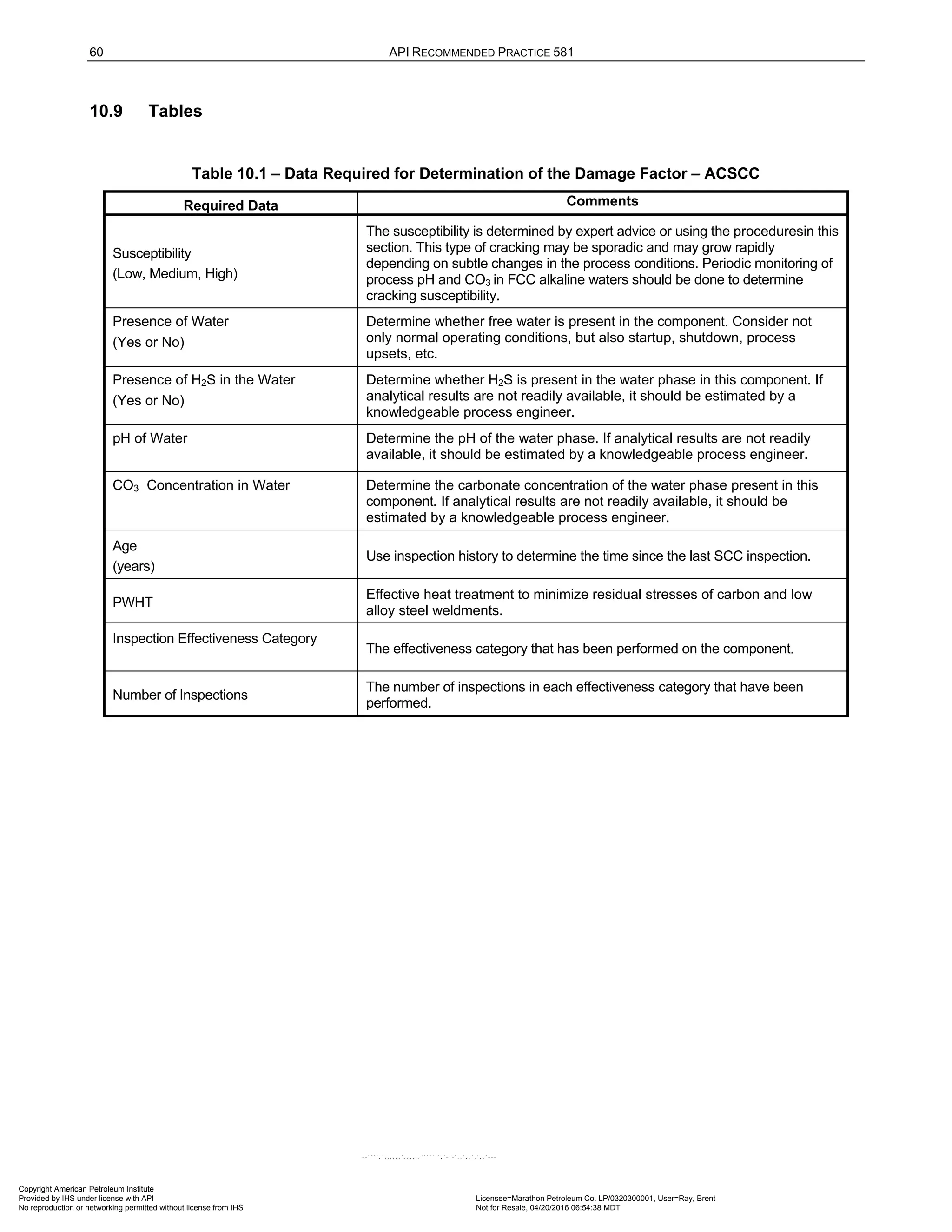
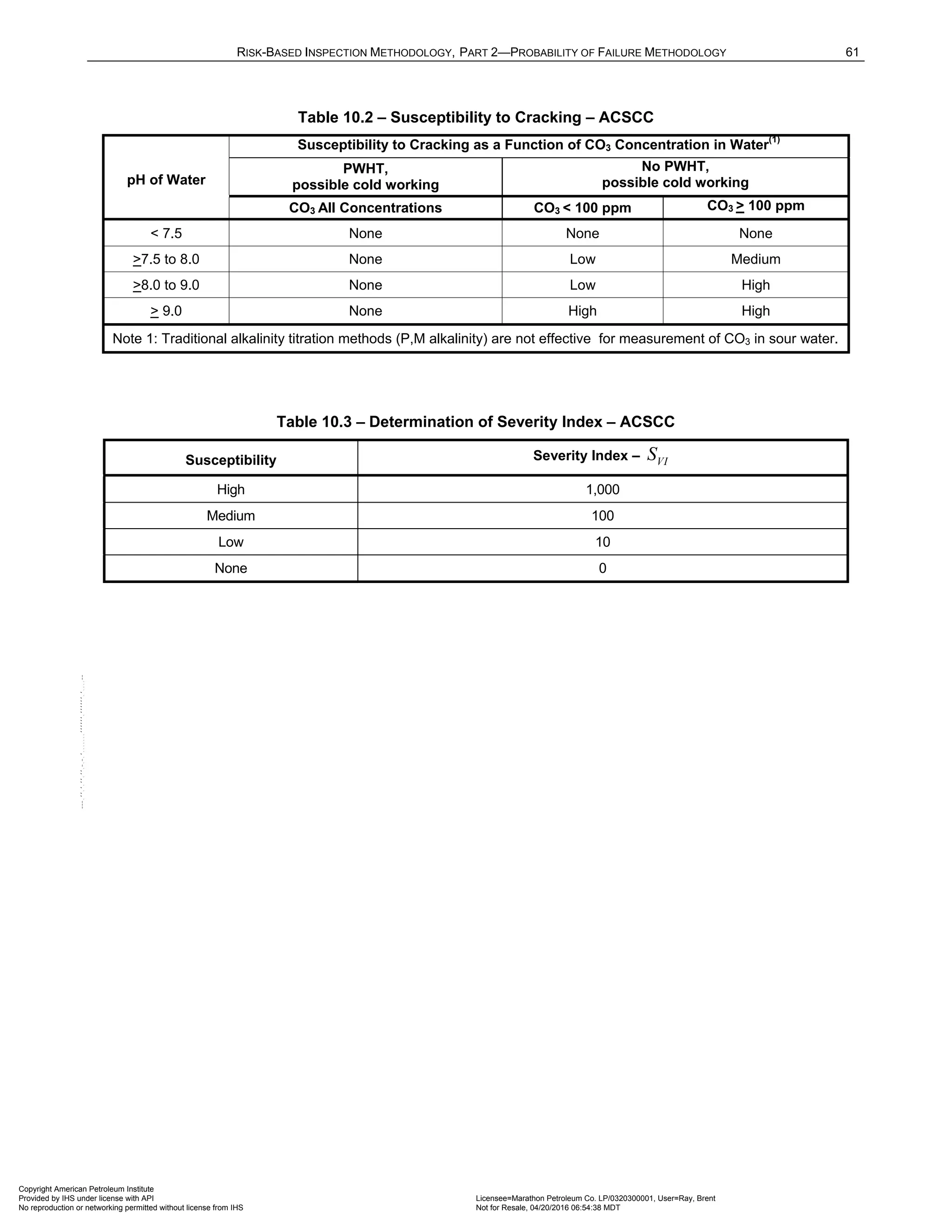

![RISK-BASED INSPECTION METHODOLOGY, PART 2—PROBABILITY OF FAILURE METHODOLOGY 63
11 Scc Damage Factor – Polythionic Acid Stress Corrosion Cracking
11.1 Scope
The DF calculation for components subject to Polythionic Acid Stress Corrosion Cracking (PASCC) is covered in
this section.
11.2 Description of Damage
Polythionic acid and sulfurous acid are major considerations in the petroleum-refining industry, particularly in
catalytic cracking, desulfurizer, hydrocracker and catalytic reforming processes. These complex acids typically
form in sulfide containing deposits during shutdown (or ambient) conditions when the component is exposed to
air and moisture. The acid environment, combined with susceptible materials of construction in the sensitized or
as-welded condition, results in rapid intergranular corrosion and cracking. Preventive measures to reduce or
eliminate PASCC include flushing the component with alkaline or soda ash solution to neutralize sulfides
immediately after shutdown and exposure to air or purging with dry nitrogen during the shutdown to prevent air
exposure, according to recommended practices established by NACE (RP0170).
Polythionic acid and sulfurous acid will cause SCC in sensitized austenitic stainless steels and nickel-base
alloys. Cracking is always intergranular and requires relatively low tensile stresses for initiation and propagation.
As-welded, regular and high carbon grade stainless steels, such as Types 304/304H and 316/316H, are
particularly susceptible to SCC in the weld heat-affected zone (HAZ). Low-carbon steels (i.e., C < 0.03%) are
less susceptible at temperatures less than 427°C (800°F). Chemically stabilized stainless steel grades, such as
Types 321 and 347 are less susceptible to PASCC, particularly if they are thermally stabilized. Susceptibility of
alloys and chemically or thermally stabilized materials to PASCC can be determined by laboratory corrosion
testing according to ASTM G35.
11.3 Screening Criteria
If the component’s material of construction is an austenitic stainless steel or nickel based alloys and the
component is exposed to sulfur bearing compounds, then the component should be evaluated for susceptibility to
PASCC.
11.4 Required Data
The basic component data required for analysis is given in Table 4.1 and the specific data required for
determination of the PASCC DF is provided in Table 11.1.
11.5 Basic Assumptions
The main assumption in determining the DF for PASCC is that the damage can be characterized by a
susceptibility parameter that is designated as high, medium, or low based on process environment, material of
construction, and component fabrication variables (i.e., heat treatment). Based on the susceptibility parameter, a
Severity Index is assigned that is a measure of the component susceptibility to cracking (or the probability of
initiating cracks) and the probability that the crack will result in a leak.
If cracks are detected in the component during an inspection, the susceptibility is designated as High, and this
will result in the maximum value for the Severity Index. Cracks that are found during an inspection should be
evaluated using Fitness-For-Service methods in API 579-1/ASME FFS-1 [13].
11.6 Determination of the Damage Factor
11.6.1 Overview
A flow chart of the steps required to determine the DF for PASCC is shown in Figure 11.1. The following
sections provide additional information and the calculation procedure.
Copyright American Petroleum Institute
Provided by IHS under license with API Licensee=Marathon Petroleum Co. LP/0320300001, User=Ray, Brent
Not for Resale, 04/20/2016 06:54:38 MDT
No reproduction or networking permitted without license from IHS
--````,`,,,,,,`,,,,,,```````,`-`-`,,`,,`,`,,`---](https://image.slidesharecdn.com/api581-3rdedition-april2016-240227010601-3bf73ab5/75/Norma-API-581-3rd-Edition-April-2016-pdf-196-2048.jpg)
![64 API RECOMMENDED PRACTICE 581
11.6.2 Inspection Effectiveness
Inspections are ranked according to their expected effectiveness at detecting for PASCC. Examples of
inspection activities that are both intrusive (requires entry into the equipment) and non-intrusive (can be
performed externally), are provided in Annex 2.C, Table 2.C.6.7.
If multiple inspections of a lower effectiveness have been conducted during the designated time period, they can
be equated to an equivalent higher effectiveness inspection in accordance with Section 3.4.3.
11.6.3 Calculation of the Damage Factor
The following procedure may be used to determine the DF for PASCC, see Figure 11.1.
a) STEP 1 – Determine the susceptibility for cracking using Figure 11.1 and Table 11.2 based on the
operating temperature and material of construction. Note that a HIGH susceptibility should be used if
cracking is confirmed to be present.
b) STEP 2 – Based on the susceptibility in STEP 1, determine the severity index, VI
S , from Table 11.3.
c) STEP 3 – Determine the time in-service, age , since the last Level A, B or C inspection was performed
with no cracking detected or cracking was repaired. Cracking detected but not repaired should be
evaluated and future inspection recommendations based upon FFS evaluation.
d) STEP 4 – Determine the number of inspections, and the corresponding inspection effectiveness category
using Section 12.9.2 for past inspections performed during the in-service time. Combine the inspections to
the highest effectiveness performed using Section 4.4.3.
e) STEP 5 – Determine the base DF for PASCC,
PASCC
fB
D , using Table 6.3 based on the number of, and the
highest inspection effectiveness determined in STEP 4, and the severity index, VI
S , from STEP 2.
f) STEP 6 – Calculate the escalation in the DF based on the time in-service since the last inspection using
the age from STEP 3 and Equation (2.30). In this equation, it is assumed that the probability for cracking
will increase with time since the last inspection as a result of increased exposure to upset conditions and
other non-normal conditions.
( )
1.1
[ ,1.0]
PASCC PASCC
f fB
D D Max age
= ⋅ (2.30)
11.7 Nomenclature
age is the component in-service time since the last cracking inspection or service start date
PASCC
f
D is the DF for PASCC cracking
PASCC
fB
D is the base value of the DF for PASCC cracking
VI
S is the severity index
11.8 References
1. Metals Handbook, Ninth Edition, ASM International, Metals Park, Ohio 44073, Volume 13 Corrosion, pp.
327.
2. D. R. McIntyre and C. P. Dillon, Guidelines for Preventing Stress Corrosion Cracking in the Chemical
Process Industries, Publication 15, Materials Technology Institute of the Chemical Process Industries, 1985,
pp. 69.
3. The Role of Stainless Steels in Petroleum Refining, American Iron and Steel Institute, 1977, pp. 42-44.
4. NACE RP0170-93, Protection of Austenitic Stainless Steels and Other Austenitic Alloys from Polythionic
Acid Stress Corrosion Cracking During Shutdown of Refinery Equipment, NACE International, Houston, TX
Copyright American Petroleum Institute
Provided by IHS under license with API Licensee=Marathon Petroleum Co. LP/0320300001, User=Ray, Brent
Not for Resale, 04/20/2016 06:54:38 MDT
No reproduction or networking permitted without license from IHS
--````,`,,,,,,`,,,,,,```````,`-`-`,,`,,`,`,,`---](https://image.slidesharecdn.com/api581-3rdedition-april2016-240227010601-3bf73ab5/75/Norma-API-581-3rd-Edition-April-2016-pdf-197-2048.jpg)
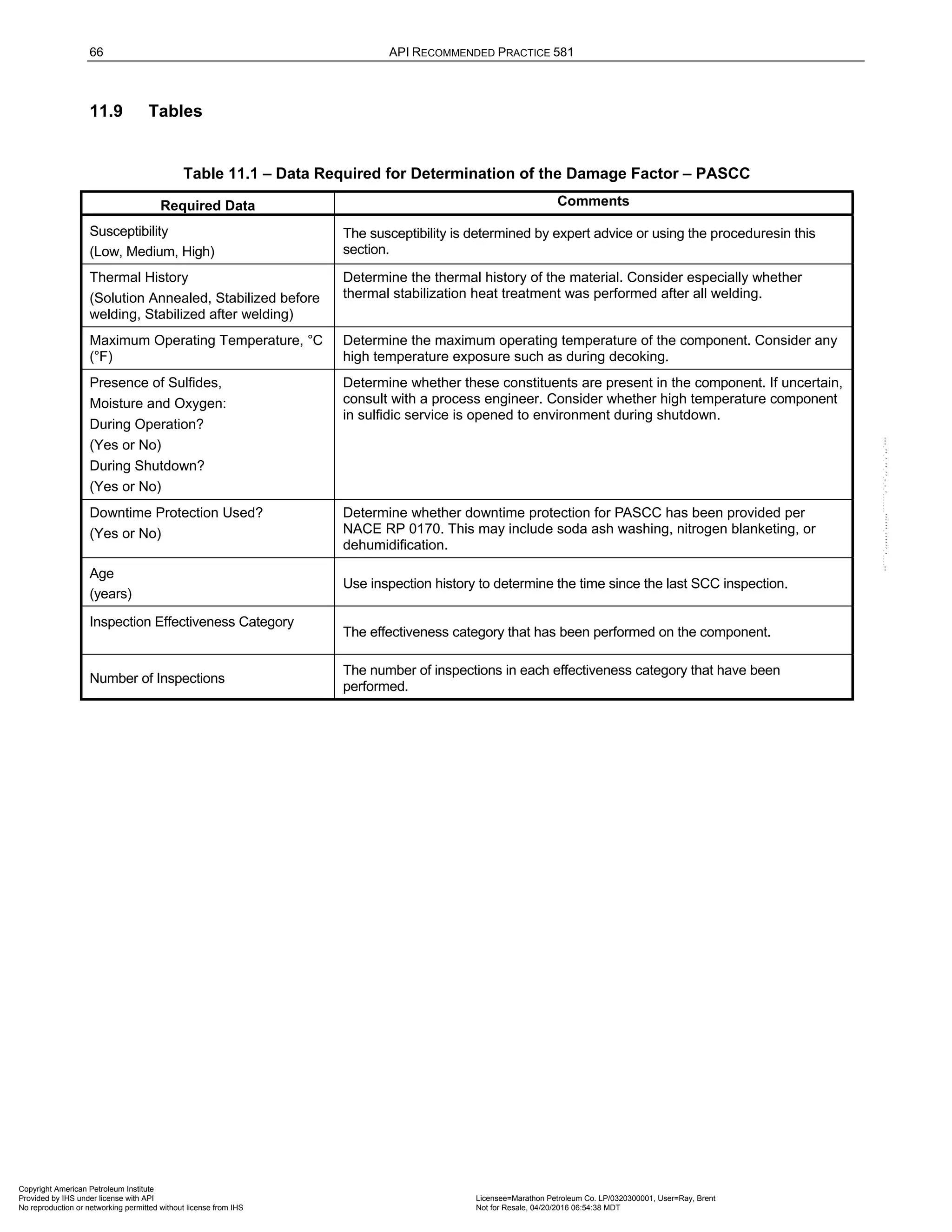
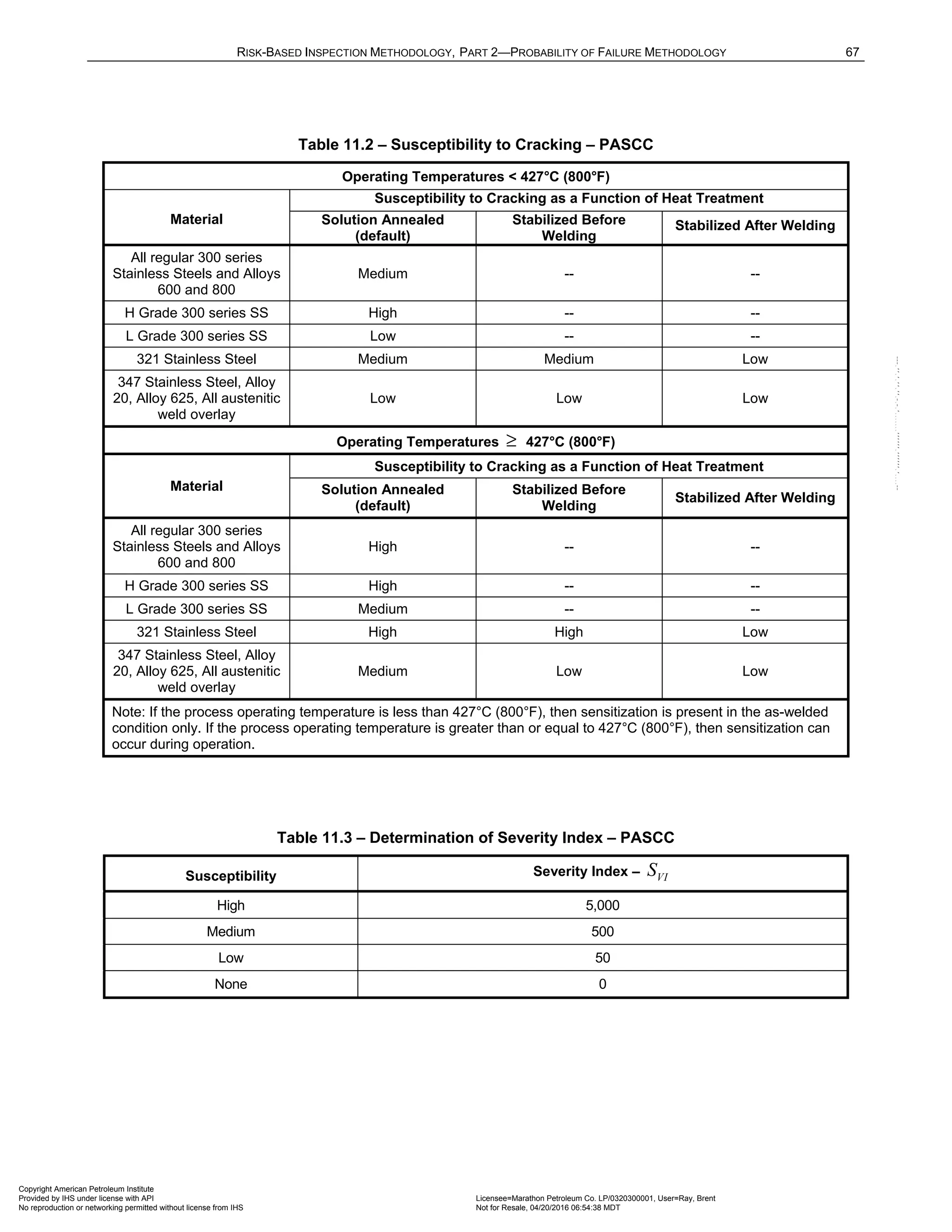
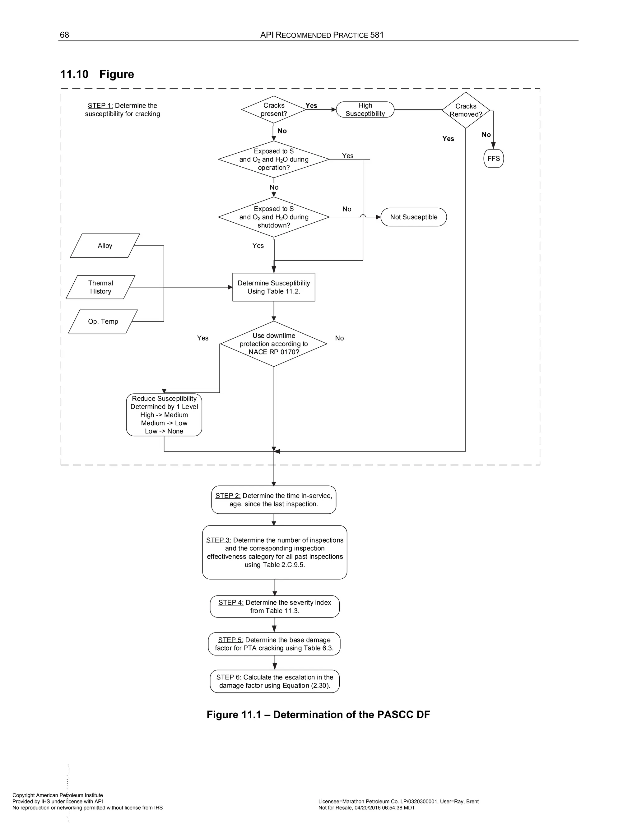
![70 API RECOMMENDED PRACTICE 581
If cracks are detected in the component during an inspection, the susceptibility is designated as High, and this
will result in the maximum value for the Severity Index. Cracks that are found during an inspection should be
evaluated using Fitness-For-Service methods in API 579-1/ASME FFS-1 [4].
12.6 Determination of the Damage Factor
12.6.1 Overview
A flow chart of the steps required to determine the DF for CLSCC is shown in Figure 12.1. The following
sections provide additional information and the calculation procedure.
12.6.2 Inspection Effectiveness
Inspections are ranked according to their expected effectiveness at detecting for CLSCC. Examples of
inspection activities that are both intrusive (requires entry into the equipment) and non-intrusive (can be
performed externally), are provided in Annex 2.C, Table 2.C.9.6.
If multiple inspections of a lower effectiveness have been conducted during the designated time period, they can
be equated to an equivalent higher effectiveness inspection in accordance with Section 3.4.3.
12.6.3 Calculation of the Damage Factor
The following procedure may be used to determine the DF for CLSCC, see Figure 12.1.
a) STEP 1 – Determine the susceptibility for cracking using Figure 12.1 and Table 12.2 based on the
operating temperature and concentration of the chloride ions. Note that a HIGH susceptibility should be
used if cracking is confirmed to be present.
b) STEP 2 – Based on the susceptibility in STEP 1, determine the severity index, VI
S , from Table 12.3.
c) STEP 3 – Determine the time in-service, age , since the last Level A, B or C inspection was performed with
no cracking detected or cracking was repaired. Cracking detected but not repaired should be evaluated and
future inspection recommendations based upon FFS evaluation.
d) STEP 4 – Determine the number of inspections, and the corresponding inspection effectiveness category
using Section 12.6.2 for past inspections performed during the in-service time. Combine the inspections to
the highest effectiveness performed using Section 3.4.3.
e) STEP 5 – Determine the base DF for CLSCC,
CLSCC
fB
D , using Table 6.3 based on the number of and the
highest inspection effectiveness determined in STEP 4, and the severity index, VI
S , from STEP 2.
f) STEP 6 – Calculate the escalation in the DF based on the time in-service since the last inspection using
the age from STEP 3 and Equation (2.31). In this equation, it is assumed that the probability for cracking
will increase with time since the last inspection as a result of increased exposure to upset conditions and
other non-normal conditions.
( )
1.1
[ ,1.0]
CLSCC CLSCC
f fB
D D Max age
= ⋅ (2.31)
12.7 Nomenclature
age is the component in-service time since the last cracking inspection or service start date
CLSCC
f
D is the DF for CLSCC
CLSCC
fB
D is the base value of the DF for CLSCC
VI
S is the severity index
Copyright American Petroleum Institute
Provided by IHS under license with API Licensee=Marathon Petroleum Co. LP/0320300001, User=Ray, Brent
Not for Resale, 04/20/2016 06:54:38 MDT
No reproduction or networking permitted without license from IHS
--````,`,,,,,,`,,,,,,```````,`-`-`,,`,,`,`,,`---](https://image.slidesharecdn.com/api581-3rdedition-april2016-240227010601-3bf73ab5/75/Norma-API-581-3rd-Edition-April-2016-pdf-203-2048.jpg)
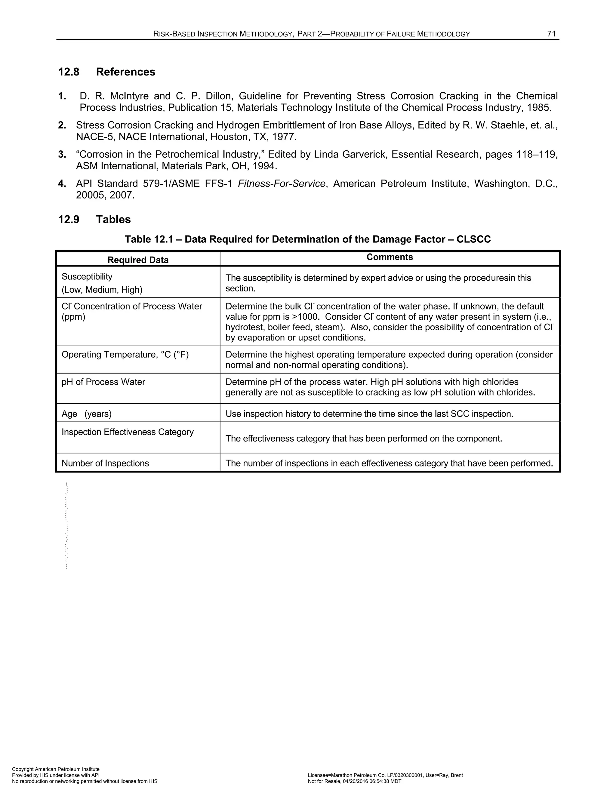
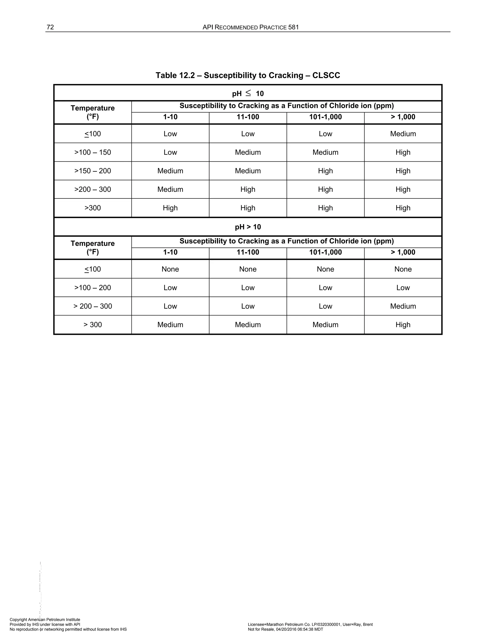
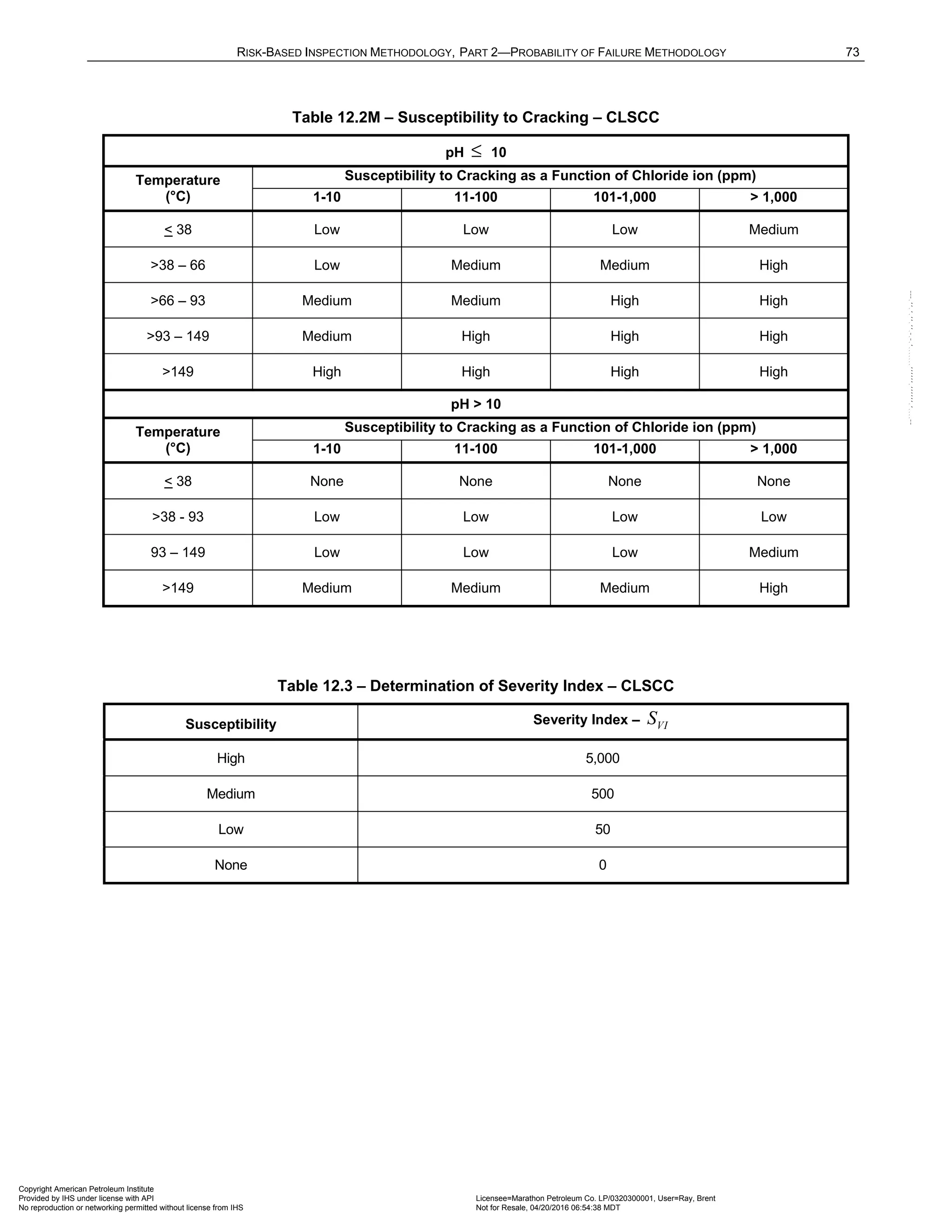
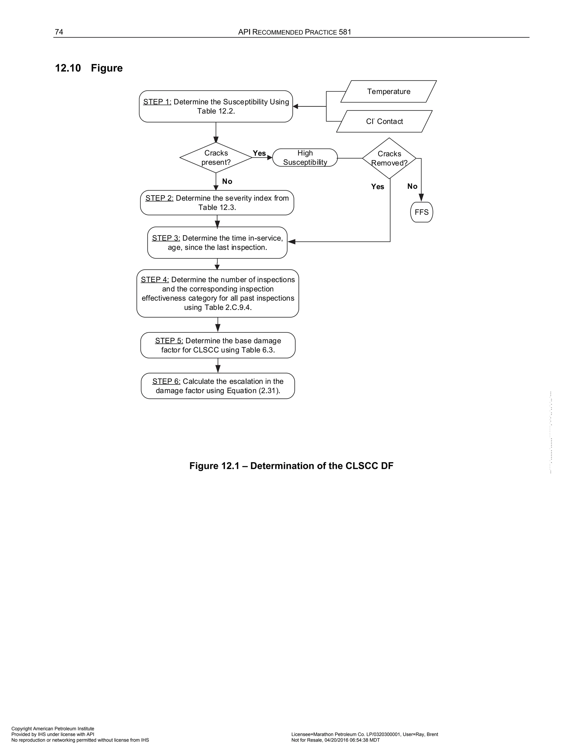
![RISK-BASED INSPECTION METHODOLOGY, PART 2—PROBABILITY OF FAILURE METHODOLOGY 75
13 Scc Damage Factor – Hydrogen Stress Cracking-Hf
13.1 Scope
The DF calculation for components subject to Hydrogen Stress Cracking in HF (HSC-HF) covered in this
section.
13.2 Description of Damage
HSC is defined as cracking of a metal under the combined action of tensile stress and a corrosion mechanism
that produces hydrogen which may diffuse into the metal. HSC may result from exposure to hydrogen sulfide,
see Section 8.0, or from exposure to hydrofluoric acid (HF). HSC-HF occurs in high-strength (high hardness)
steels or in hard weld deposits or hard heat-affected zones (HAZs) of lower-strength steels. In addition, HSC-HF
may occur in stressed Alloy 400 if oxygen or other oxidizers are present in the HF.
Concentrated hydrofluoric acid (HF) is used as the acid catalyst in HF alkylation units. The usual HF-in-water
concentrations are 96%–99+% and the temperatures are generally below 66°C (150°F). Under these conditions
a fully killed (deoxidized), low sulfur, clean soft carbon steel is the material of choice for most equipment except
where close tolerances are required for operation (i.e., pumps, valves, instruments).
Where close tolerances are required and at temperatures over 66°C (150°F) to approximately 178°C (350°F),
Alloy 400 is used. Corrosion in 80% and stronger HF-in-water solutions is equivalent to corrosion in anhydrous
hydrofluoric acid (AHF, <200 ppm H20) and reference to corrosion in AHF implies an HF-in-water concentration
as low as 80%. HF acid with a concentration lower than 80% HF in water is considered aqueous. Both aqueous
and anhydrous HF can cause hydrogen embrittlement of hardened carbon and alloy steels. To prevent
hydrogen embrittlement in welded steel structures, the requirements of NACE RP 0472, Methods and Controls
to Prevent In-Service Cracking of Carbon Steel Welds in Corrosive Petroleum Refining Environments should be
followed. Welds produced by all welding methods should be hardness tested.
Alloy steel fasteners have been a source of many failures in anhydrous HF service. ASTM A193 Grade B7,
chromium molybdenum steel bolts are hard and will crack in the presence of HF. Grade B7M, the same steel
tempered to a lower hardness of 201–235 Brinnell may be a better choice if contact by HF cannot be avoided.
However, B7M bolts will also crack if stressed beyond their yield point in an HF environment. Bolt torque may be
difficult to control in field flange make-up. In this case, B7 bolts may be specified and replacement of any bolt
which may have contacted HF as a result of flange leaks would be required.
13.3 Screening Criteria
If the component’s material of construction is carbon or low alloy steel and the component is exposed to
hydrofluoric acid in any concentration, then the component should be evaluated for susceptibility to HSC-HF.
13.4 Required Data
The basic component data required for analysis is given in Table 4.1 and the specific data required for
determination of the HSC-HF DF is provided in Table 13.1.
13.5 Basic Assumptions
The main assumption in determining the DF for HSC-HF is that the damage can be characterized by a
susceptibility parameter that is designated as high, medium, or low based on process environment, material of
construction, and component fabrication variables (i.e., heat treatment). Based on the susceptibility parameter, a
Severity Index is assigned that is a measure of the component susceptibility to cracking (or the probability of
initiating cracks) and the probability that the crack will result in a leak.
If cracks are detected in the component during an inspection, the susceptibility is designated as High, and this
will result in the maximum value for the Severity Index. Cracks that are found during an inspection should be
evaluated using Fitness-For-Service methods in API 579-1/ASME FFS-1 [3].
Copyright American Petroleum Institute
Provided by IHS under license with API Licensee=Marathon Petroleum Co. LP/0320300001, User=Ray, Brent
Not for Resale, 04/20/2016 06:54:38 MDT
No reproduction or networking permitted without license from IHS
--````,`,,,,,,`,,,,,,```````,`-`-`,,`,,`,`,,`---](https://image.slidesharecdn.com/api581-3rdedition-april2016-240227010601-3bf73ab5/75/Norma-API-581-3rd-Edition-April-2016-pdf-208-2048.jpg)
![76 API RECOMMENDED PRACTICE 581
13.6 Determination of the Damage Factor
13.6.1 Overview
A flow chart of the steps required to determine the DF for HSC-HF is shown in Figure 13.1. The following
sections provide additional information and the calculation procedure.
13.6.2 Inspection Effectiveness
Inspections are ranked according to their expected effectiveness at detecting for HSC. Examples of inspection
activities that are both intrusive (requires entry into the equipment) and non-intrusive (can be performed
externally), are provided in Annex 2.C, Table 2.C.9.8.
If multiple inspections of a lower effectiveness have been conducted during the designated time period, they can
be equated to an equivalent higher effectiveness inspection in accordance with Section 3.4.3.
13.6.3 Calculation of the Damage Factor
The following procedure may be used to determine the DF for HSC-HF, see Figure 13.1.
a) STEP 1 – Determine the susceptibility for cracking using Figure 13.1 and Table 13.2 based on the
maximum Brinnell hardness of weldments, and knowledge of whether the component was subject to
PWHT. Note that a HIGH susceptibility should be used if cracking is confirmed to be present.
b) STEP 2 – Based on the susceptibility in STEP 1, determine the severity index, VI
S , from Table 13.3.
c) STEP 3 – Determine the time in-service, age , since the last Level A, B or C inspection was performed
with no cracking detected or cracking was repaired. Cracking detected but not repaired should be
evaluated and future inspection recommendations based upon FFS evaluation.
d) STEP 4 – Determine the number of inspections, and the corresponding inspection effectiveness category
using Section 13.6.2 for past inspections performed during the in-service time. Combine the inspections to
the highest effectiveness performed using Section 3.4.3.
e) STEP 5 – Determine the base DF for HSC-HF,
HSC HF
fB
D −
, using Table 6.3 based on the number of, and the
highest inspection effectiveness determined in STEP 4, and the severity index, VI
S , from STEP 2.
f) STEP 6 – Calculate the escalation in the DF based on the time in-service since the last inspection using
the age from STEP 3 and Equation (2.32). In this equation, it is assumed that the probability for cracking
will increase with time since the last inspection as a result of increased exposure to upset conditions and
other non-normal conditions.
( )
1.1
[ ,1.0]
HSC HF HSC HF
f fB
D D Max age
− −
= ⋅ (2.32)
13.7 Nomenclature
age is the component in-service time since the last cracking inspection or service start date
HSC HF
f
D −
is the DF for HSC-HF
HSC HF
fB
D −
is the base value of the DF for HSC-HF
VI
S is the severity index
Copyright American Petroleum Institute
Provided by IHS under license with API Licensee=Marathon Petroleum Co. LP/0320300001, User=Ray, Brent
Not for Resale, 04/20/2016 06:54:38 MDT
No reproduction or networking permitted without license from IHS
--````,`,,,,,,`,,,,,,```````,`-`-`,,`,,`,`,,`---](https://image.slidesharecdn.com/api581-3rdedition-april2016-240227010601-3bf73ab5/75/Norma-API-581-3rd-Edition-April-2016-pdf-209-2048.jpg)
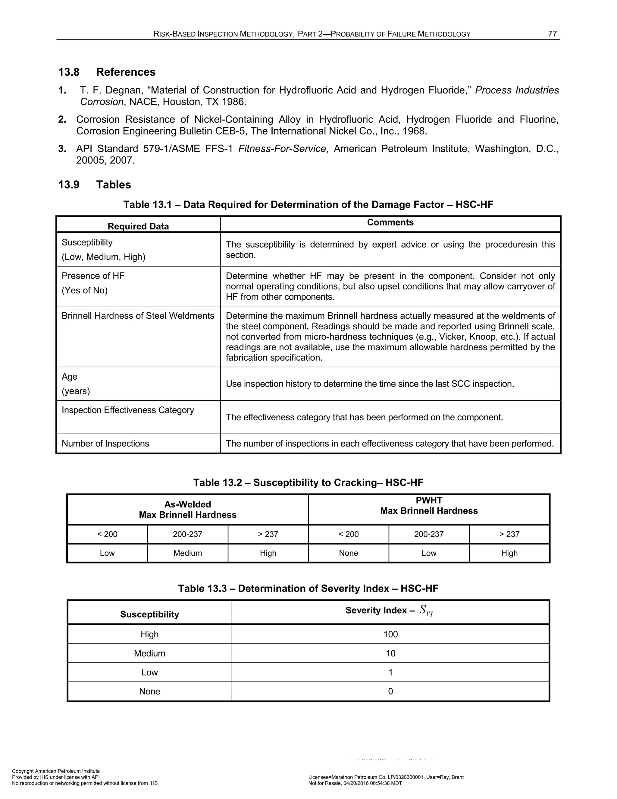
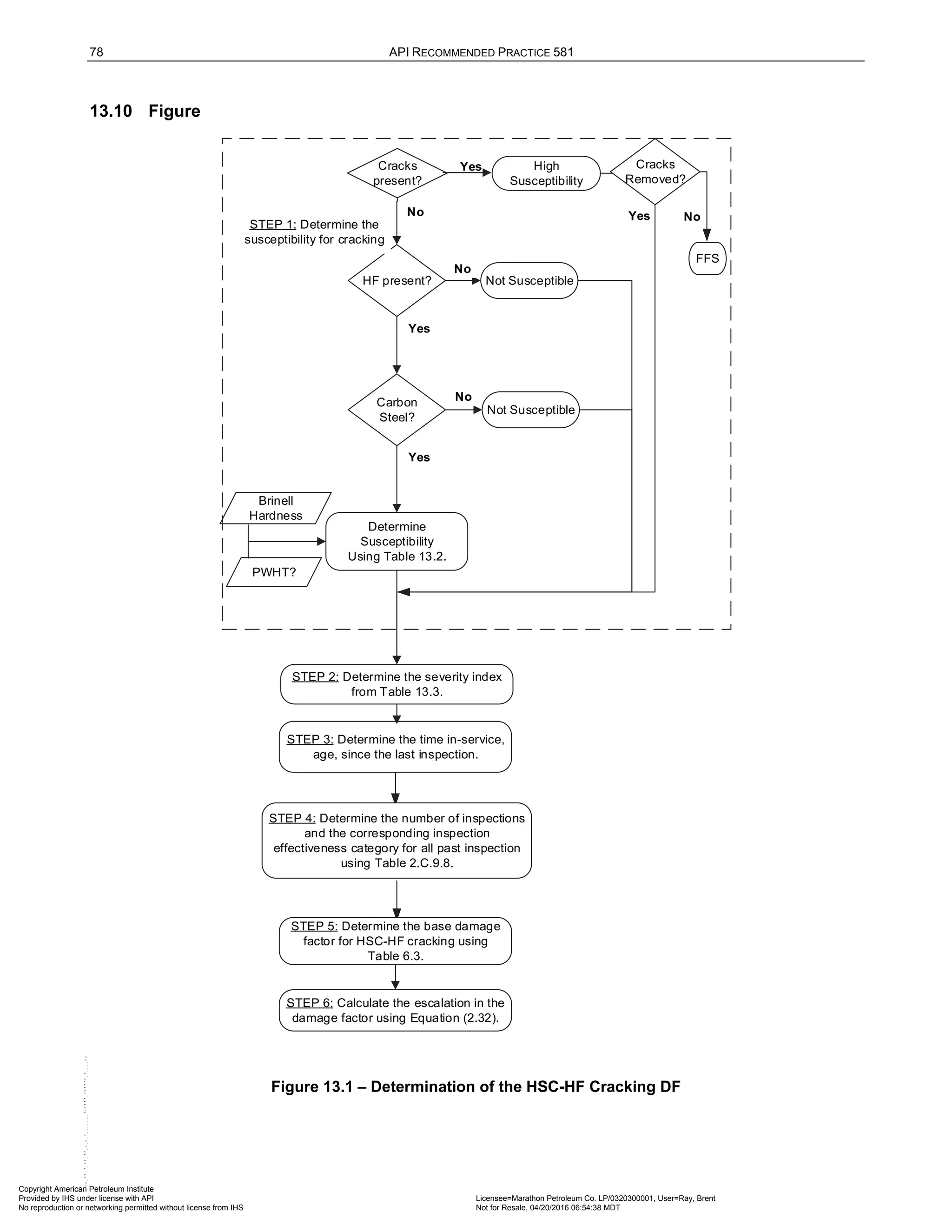
![80 API RECOMMENDED PRACTICE 581
Piping fabricated from wrought components of conventional steels (i.e., A 53, A 106, API 5L [not including 5LX],
A 234, A 105, etc.) should be considered to have a low susceptibility to HIC/SOHIC-HF. For components
fabricated from rolled and welded plate steel, the susceptibility should be determined using Table 14.4. The
susceptibility of the steel to blistering is directly related to the cleanliness of the steel. It should be recognized
that blistering is not a damage mechanism which will lead to a leak path unless it is accompanied by hydrogen-
induced cracking leading to the surface. Blistering does pose a danger to mechanical integrity particularly when
it approaches a weld which contains sufficient residual stresses to drive the hydrogen-induced cracking to the
surfaces. It is this last case, the most severe situation that is considered when determining the susceptibility to
HIC/SOHIC-HF.
If cracks are detected in the component during an inspection, the susceptibility is designated as High, and this
will result in the maximum value for the Severity Index. Cracks that are found during an inspection should be
evaluated using Fitness-For-Service methods in API 579-1/ASME FFS-1 [3].
14.6 Determination of the Damage Factor
14.6.1 Overview
A flow chart of the steps required to determine the DF for HIC/SOHIC-HF is shown in Figure 14.1. The following
sections provide additional information and the calculation procedure.
14.6.2 Inspection Effectiveness
Inspections are ranked according to their expected effectiveness at detecting for HIC/SOHIC-HF. Examples of
inspection activities that are both intrusive (requires entry into the equipment) and non-intrusive (can be
performed externally), are provided in Annex 2.C, Table 2.C.9.9.
If multiple inspections of a lower effectiveness have been conducted during the designated time period, they can
be equated to an equivalent higher effectiveness inspection in accordance with Section 3.4.3.
14.6.3 Adjustment for On-Line Monitoring
In addition to inspection, on-line monitoring using hydrogen probes and/or key process variables provides a
better understanding of HIC/SOHIC-HF susceptibility. The advantage of on-line monitoring is that process
changes affecting SCC susceptibility can be detected before significant cracking occurs. This earlier detection
could permit more timely action to decrease the POF. For HIC/SOHIC-HF, an on-line monitoring factor of 2 is
applied if either hydrogen probes or monitoring of key process variables are used. If both hydrogen probes and
monitoring of key process variables are used, an on-line monitoring factor is 4 is applied.
14.6.4 Calculation of the Damage Factor
The following procedure may be used to determine the DF for HIC/SOHIC-HF, see Figure 14.1.
a) STEP 1 – Determine the susceptibility for cracking using Figure 14.1 and Table 14.2 based on the material
of construction and knowledge of whether the component was subject to PWHT. Note that a HIGH
susceptibility should be used if cracking is confirmed to be present.
b) STEP 2 – Based on the susceptibility in STEP 1, determine the severity index, VI
S , from Table 14.3. In
determining the susceptibility, it should be noted that if HF is present in any concentration, then the
component is potentially susceptible to HIC/SOHIC-HF.
c) STEP 3 – Determine the time in-service, age , since the last Level A, B or C inspection was performed
with no cracking detected or cracking was repaired. Cracking detected but not repaired should be
evaluated and future inspection recommendations based upon FFS evaluation.
d) STEP 4 – Determine the number of inspections, and the corresponding inspection effectiveness category
using Section 14.6.2 for past inspections performed during the in-service time. Combine the inspections to
the highest effectiveness performed using Section 3.4.3.
e) STEP 5 – Determine the base DF for HIC/SOHIC-HF,
/
HIC SOHIC HF
fb
D −
, using Table 6.3 based on the
number of, and the highest inspection effectiveness determined in STEP 4, and the severity index, VI
S ,
from STEP 2.
Copyright American Petroleum Institute
Provided by IHS under license with API Licensee=Marathon Petroleum Co. LP/0320300001, User=Ray, Brent
Not for Resale, 04/20/2016 06:54:38 MDT
No reproduction or networking permitted without license from IHS
--````,`,,,,,,`,,,,,,```````,`-`-`,,`,,`,`,,`---](https://image.slidesharecdn.com/api581-3rdedition-april2016-240227010601-3bf73ab5/75/Norma-API-581-3rd-Edition-April-2016-pdf-213-2048.jpg)
![RISK-BASED INSPECTION METHODOLOGY, PART 2—PROBABILITY OF FAILURE METHODOLOGY 81
f) STEP 6 – Determine the on-line adjustment factor, OM
F , from Table 15.4.
g) STEP 7 – Calculate the final DF accounting for escalation based on the time in-service since the last
inspection using the age from STEP 3 and Equation (2.33). In this equation, it is assumed that the
probability for cracking will increase with time since the last inspection as a result of increased exposure to
upset conditions and other non-normal conditions. The equation also applies the adjustment factor for on-
line monitoring.
( )
1.1
/
/ [ ,1.0]
HIC SOHIC HF
fB
HIC SOHIC HF
f
OM
D Max age
D
F
−
− ⋅
= (2.33)
14.7 Nomenclature
age is the component in-service time since the last cracking inspection or service start date
/
HIC SOHIC HF
f
D −
is the DF for HIC/SOHIC-HF
/
HIC SOHIC HF
fB
D −
is the base value of the DF for HIC/SOHIC-HF
OM
F is the on-line monitoring adjustment factor
VI
S is the severity index
14.8 References
1. T. F. Degnan, “Material of Construction for Hydrofluoric Acid and Hydrogen Fluoride,” Process Industries
Corrosion, NACE, Houston, TX 1986.
2. Corrosion Resistance of Nickel-Containing Alloy in Hydrofluoric Acid, Hydrogen Fluoride and Fluorine,
Corrosion Engineering Bulletin CEB-5, The International Nickel Co., Inc., 1968.
3. API STD 579-1/ASME FFS-1 Fitness-For-Service, American Petroleum Institute, Washington, D.C., 20005,
2007.
Copyright American Petroleum Institute
Provided by IHS under license with API Licensee=Marathon Petroleum Co. LP/0320300001, User=Ray, Brent
Not for Resale, 04/20/2016 06:54:38 MDT
No reproduction or networking permitted without license from IHS
--````,`,,,,,,`,,,,,,```````,`-`-`,,`,,`,`,,`---](https://image.slidesharecdn.com/api581-3rdedition-april2016-240227010601-3bf73ab5/75/Norma-API-581-3rd-Edition-April-2016-pdf-214-2048.jpg)
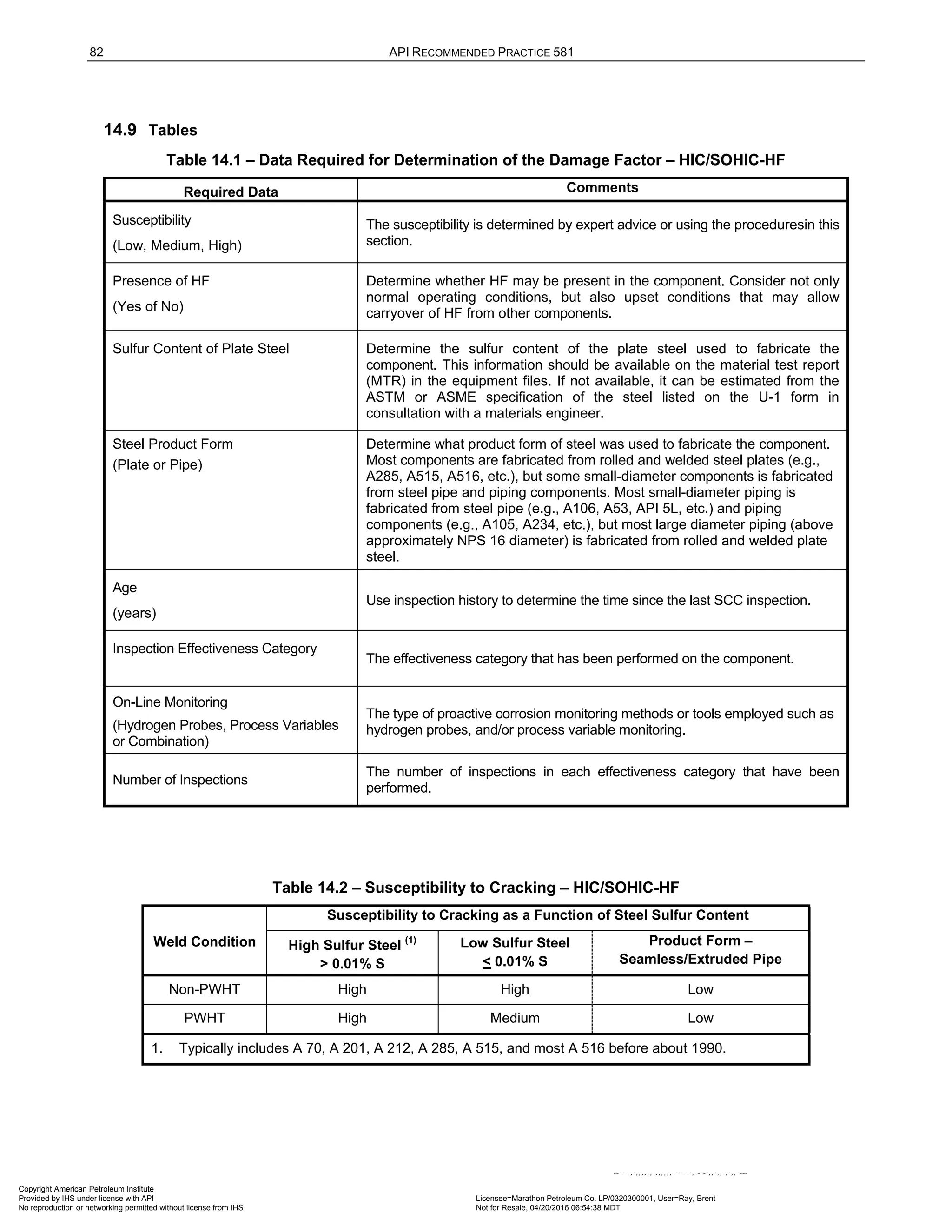
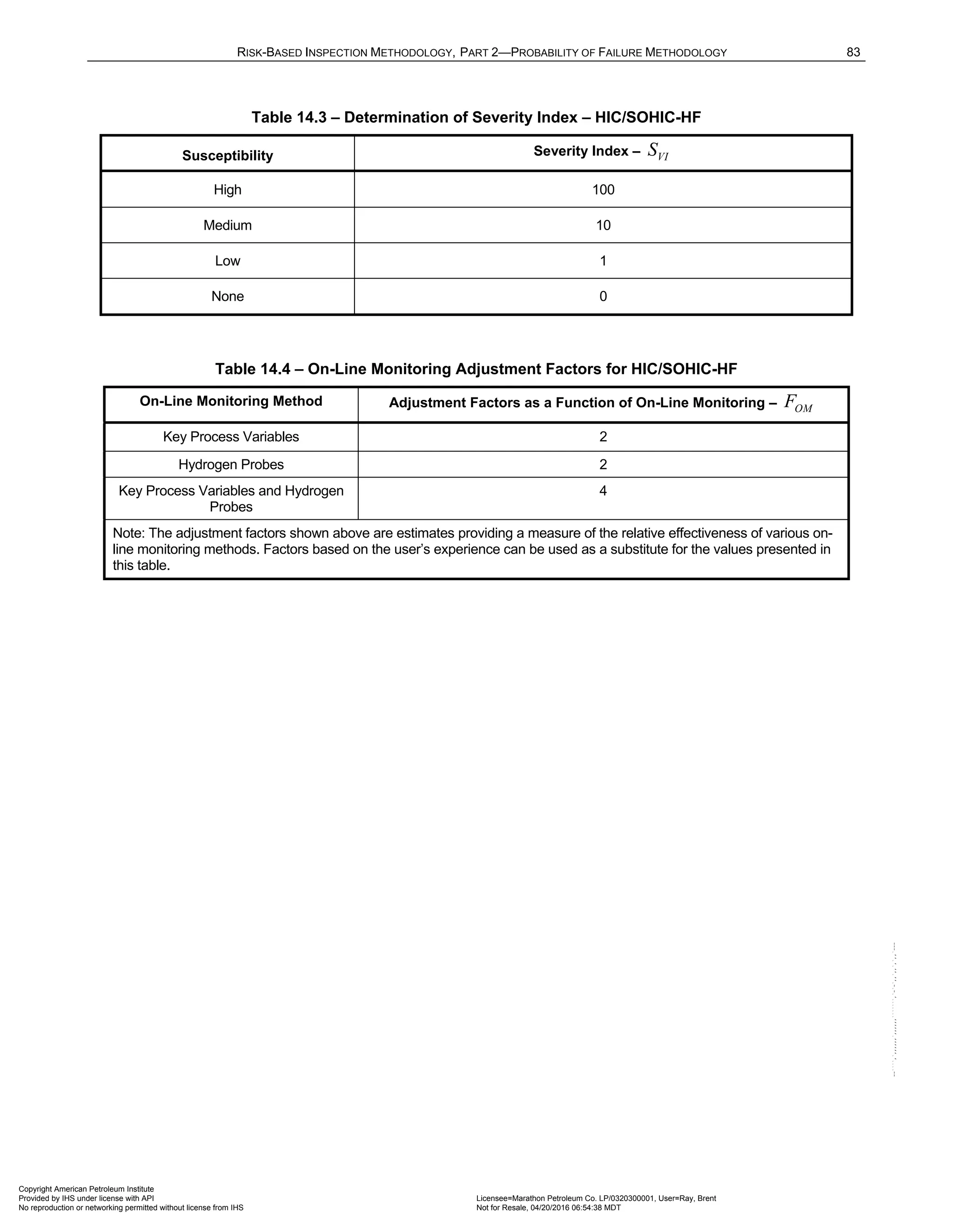
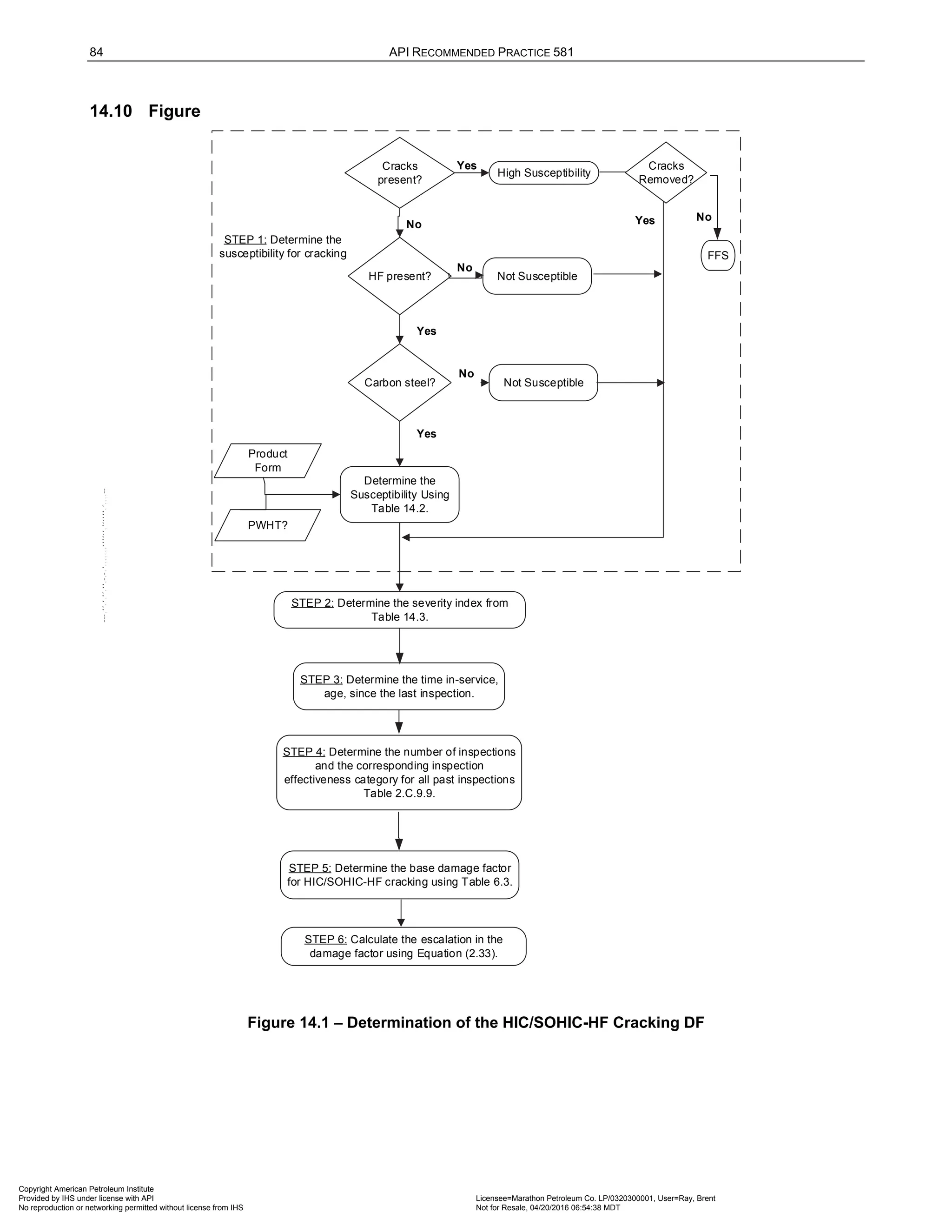
![86 API RECOMMENDED PRACTICE 581
15.6.3 Calculation of the Damage Factor
The following procedure may be used to determine the DF for external corrosion, see Figure 15.1.
a) STEP 1 – Determine the furnished thickness, t , and age, age , for the component from the installation
date.
b) STEP 2 – Determine the base corrosion rate, rB
C , based on the driver and operating temperature using
Table 15.2.
c) STEP 3 – Calculate the final corrosion rate, r
C , using Equation (2.34).
max ,
r rB EQ IF
C C F F
= ⋅ (2.34)
The adjustment factors are determined as follows.
1) Adjustment for Equipment Design or Fabrication, EQ
F – If the equipment has a design which allows water
to pool and increase metal loss rates, such as piping supported directly on beams, vessel stiffening rings or
insulation supports or other such configuration that does not allow water egress and/or does not allow for
proper coating maintenance, then 2
EQ
F = ; otherwise, 1
EQ
F = .
2) Adjustment for Interface, IF
F – If the piping has an interface where it enters either soil or water, then
2
IF
F = ; otherwise, 1
IF
F = .
d) STEP 4 – Determine the time in-service, tk
age , since the last known inspection thickness, rde
t (see Section
4.5.5. The rde
t is the starting thickness with respect to wall loss associated with external corrosion. If no
measured thickness is available, set rde
t t
= and tk
age age
= .
e) STEP 5 – Determine the in-service time, coat
age , since the coating has been installed using Equation
(2.35).
coat
age Calculation Date Coating Installation Date
= − (2.35)
f) STEP 6 – Determine coating adjustment, adj
Coat , using Equations (2.36) through (2.41).
If :
tk coat
age age
≥
0
adj
Coat No Coating or Poor Coating Quality
=
(2.36)
[ ]
min 5,
adj coat
Coat age Medium Coating Quality
= (2.37)
[ ]
min 15,
adj coat
Coat age High Coating Quality
= (2.38)
If :
tk coat
age age
<
0
adj
Coat No Coating or Poor Coating Quality
=
(2.39)
[ ] [ ]
min 5, min 5,
adj coat coat tk
Coat age age age Medium Coating Quality
= − − (2.40)
[ ] [ ]
min 15, min 15,
adj coat coat tk
Coat age age age High Coating Quality
= − − (2.41)
g) STEP 7 – Determine the in-service time, age , over which external corrosion may have occurred using
Equation (2.42).
tk adj
age age Coat
= − (2.42)
Copyright American Petroleum Institute
Provided by IHS under license with API Licensee=Marathon Petroleum Co. LP/0320300001, User=Ray, Brent
Not for Resale, 04/20/2016 06:54:38 MDT
No reproduction or networking permitted without license from IHS
--````,`,,,,,,`,,,,,,```````,`-`-`,,`,,`,`,,`---](https://image.slidesharecdn.com/api581-3rdedition-april2016-240227010601-3bf73ab5/75/Norma-API-581-3rd-Edition-April-2016-pdf-219-2048.jpg)
![RISK-BASED INSPECTION METHODOLOGY, PART 2—PROBABILITY OF FAILURE METHODOLOGY 87
h) STEP 8 – Determine the allowable stress, S , weld joint efficiency, E , and minimum required thickness,
min
t , per the original construction code or API 579-1/ASME FFS-1 [10]. In cases where components are
constructed of uncommon shapes or where the component's minimum structural thickness, c
t , may govern,
the user may use the c
t in lieu of min
t where pressure does not govern the minimum required thickness
criteria.
i) STEP 9 - Determine the rt
A parameter using Equation (2.43) based on the age and rde
t from STEP 4,
r
C from STEP 3.
r
rt
rde
C age
A
t
⋅
=
(2.43)
j) STEP 10 – Calculate the Flow Stress, extcorr
FS , using S from STEP 8 and Equation (2.44).
( ) 1.1
2
extcorr YS TS
FS E
+
= ⋅ ⋅ (2.44)
Note: Use Flow Stress ( Thin
FS ) at design temperature for conservative results, using the appropriate
Equation (2.45) or (2.46).
k) STEP 11 – Calculate the strength ratio parameter, Thin
P
SR , using Equation (2.45) or (2.46).
1) Use Equation (2.45) with rde
t from STEP 3, min
t or c
t , S and E from STEP 8, and extcorr
FS from STEP 10.
min
( , )
extcorr c
P extcorr
rde
S E Max t t
SR
FS t
⋅
= ⋅ (2.45)
Note: The min
t is based on a design calculation that includes evaluation for internal pressure hoop
stress, external pressure and/or structural considerations, as appropriate. The minimum required
thickness calculation is the design code min
t . Consideration for internal pressure hoop stress alone
may not be sufficient. c
t as defined in STEP 5 may be used when appropriate.
2) Using Equation (2.46) with rde
t from STEP 4 and extcorr
FS from STEP 10.
extcorr
P extcorr
rde
P D
SR
FS t
α
⋅
=
⋅ ⋅
(2.46)
Where α is the shape factor for the component type
2 ,4 ,1.13
for a cylinder for a sphere for a head
α = .
Note: This strength ratio parameter is based on internal pressure hoop stress only. It is not
appropriate where external pressure and/or structural considerations dominate. . When c
t dominates
or if the min
t is calculated using another method, Equation (2.45) should be used.
l) STEP 12 – Determine the number of inspections, extcorr
A
N , extcorr
B
N , extcorr
C
N , extcorr
D
N , and the
corresponding inspection effectiveness category using Section 15.6.2 for past inspections performed during
the in-service time (see Section 4.5.5).
Copyright American Petroleum Institute
Provided by IHS under license with API Licensee=Marathon Petroleum Co. LP/0320300001, User=Ray, Brent
Not for Resale, 04/20/2016 06:54:38 MDT
No reproduction or networking permitted without license from IHS
--````,`,,,,,,`,,,,,,```````,`-`-`,,`,,`,`,,`---](https://image.slidesharecdn.com/api581-3rdedition-april2016-240227010601-3bf73ab5/75/Norma-API-581-3rd-Edition-April-2016-pdf-220-2048.jpg)
![88 API RECOMMENDED PRACTICE 581
m) STEP 13 – Determine the inspection effectiveness factors, 1
extcorr
I , 2
extcorr
I , 3
extcorr
I , using Equation
(2.47), Prior Probabilities, 1
extcorr
p
Pr , 2
extcorr
p
Pr and 3
extcorr
p
Pr , from Table 4.5, Conditional Probabilities (for each
inspection effectiveness level), 1
extcorr
p
Co , 2
extcorr
p
Co and 3
extcorr
p
Co , from Table 4.6, and the number of
inspections inspections, extcorr
A
N , extcorr
B
N , extcorr
C
N , extcorr
D
N , in each effectiveness level obtained from STEP
12.
( ) ( ) ( ) ( )
( ) ( ) ( )
1 1 1 1 1 1
2 2 2 2 2 2
extcorr extcorr extcorr extcorr
A B C D
extcorr extcorr extcorr
A B C
N N N N
extcorr extcorr extcorrA extcorrB extcorrC extcorrD
p p p p p
N N N
extcorr extcorr extcorrA extcorrB extcorrC extcorr
p p p p p
I Pr Co Co Co Co
I Pr Co Co Co Co
=
= ( )
( ) ( ) ( ) ( )
3 3 3 3 3 3
extcorr
D
extcorr extcorr extcorr extcorr
A B C D
N
D
N N N N
extcorr extcorr extcorrA extcorrB extcorrC extcorrD
p p p p p
I Pr Co Co Co Co
=
(2.47)
p) STEP 14 – Calculate the Posterior Probabilities, 1
extcorr
p
Po , 2
extcorr
p
Po and 3
extcorr
p
Po using Equation (2.48)
with 1
extcorr
I , 2
extcorr
I and 3
extcorr
I in Step 12.
1
1
1 2 3
2
2
1 2 3
3
3
1 2 3
extcorr
extcorr
p extcorr extcorr extcorr
extcorr
extcorr
p extcorr extcorr extcorr
extcorr
extcorr
p extcorr extcorr extcorr
I
Po
I I I
I
Po
I I I
I
Po
I I I
=
+ +
=
+ +
=
+ +
(2.48)
q) STEP 15 – Calculate the parameters, 1 2 3
, ,
extcorr extcorr extcorr
β β β using Equation (2.49) and assigning
0.20
t
COVΔ = , 0.20
f
S
COV = and 0.05
P
COV = .
( )
( )
1
1 1
2
2 2
3
1 2
2 2 2 2 2 2
2 2
2 2 2 2 2 2
3
1
,
1 ( )
1
,
1 ( )
1
f
f
extcorr
S rt p
extcorr
extcorr
S rt t S rt S p P
extcorr
S rt p
extcorr
extcorr
S rt t S rt S p P
extcorr
S rt p
extcorr
D A SR
D A COV D A COV SR COV
D A SR
D A COV D A COV SR COV
D A SR
β
β
β
Δ
Δ
− ⋅ −
=
⋅ ⋅ + − ⋅ ⋅ + ⋅
− ⋅ −
=
⋅ ⋅ + − ⋅ ⋅ + ⋅
− ⋅ −
=
( )
3 3
2
2 2 2 2 2 2
.
1 ( )
f
extcorr
S rt t S rt S p P
D A COV D A COV SR COV
Δ
⋅ ⋅ + − ⋅ ⋅ + ⋅
(2.49)
Where 1
1
S
D = , 2
2
S
D = and 3
4
S
D = . These are the corrosion rate factors for damage states 1, 2 and 3 as
as discussed in 4.5.3 [35]. Note that the DF calculation is very sensitive to the value used for the
coefficient of variance for thickness, t
COVΔ . The t
COVΔ is in the range 0.10 0.20
t
COVΔ
≤ ≤ , with a
recommended conservative value of 0.20
t
COVΔ = .
r) STEP 16 – Calculate
extcorr
f
D using Equation (2.50).
( )
( ) ( )
( ) ( )
( )
1 1 2 2 3 3
1.56 04
extcorr extcorr extcorr extcorr extcorr extcorr
p p p
extcorr
f
Po Po Po
D
E
β β β
Φ − + Φ − + Φ −
=
−
(2.50)
Where Φ is the standard normal cumulative distribution function (NORMSDIST in Excel).
Copyright American Petroleum Institute
Provided by IHS under license with API Licensee=Marathon Petroleum Co. LP/0320300001, User=Ray, Brent
Not for Resale, 04/20/2016 06:54:38 MDT
No reproduction or networking permitted without license from IHS
--````,`,,,,,,`,,,,,,``](https://image.slidesharecdn.com/api581-3rdedition-april2016-240227010601-3bf73ab5/75/Norma-API-581-3rd-Edition-April-2016-pdf-221-2048.jpg)

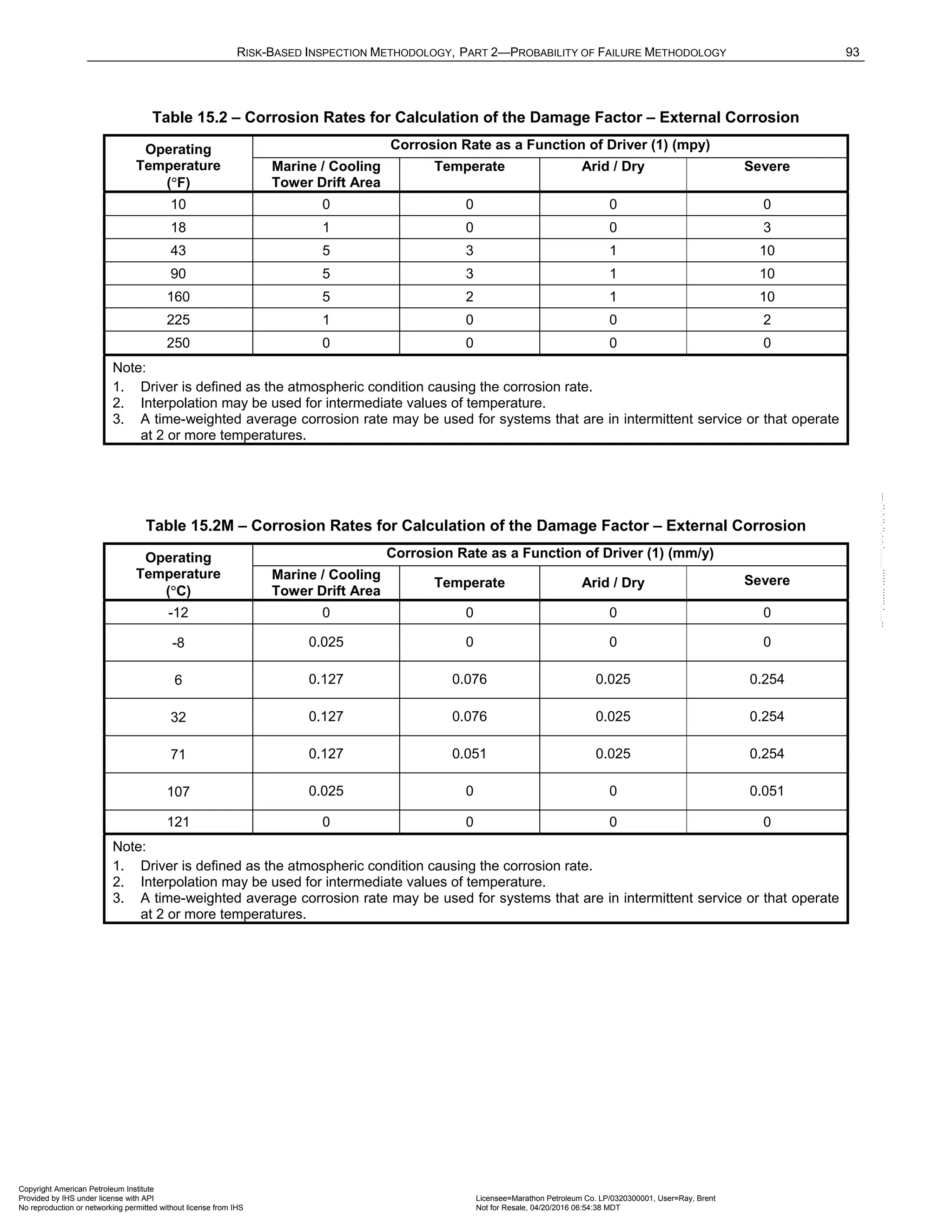
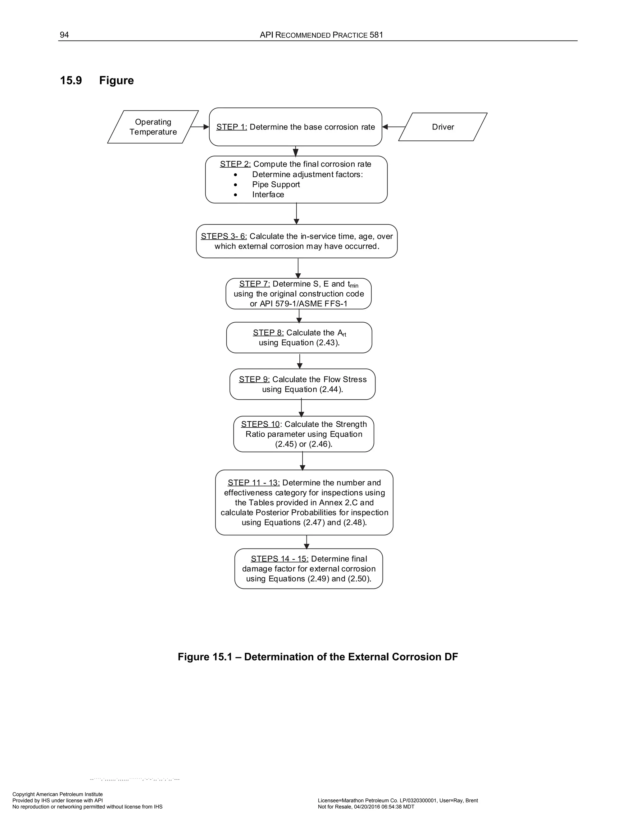
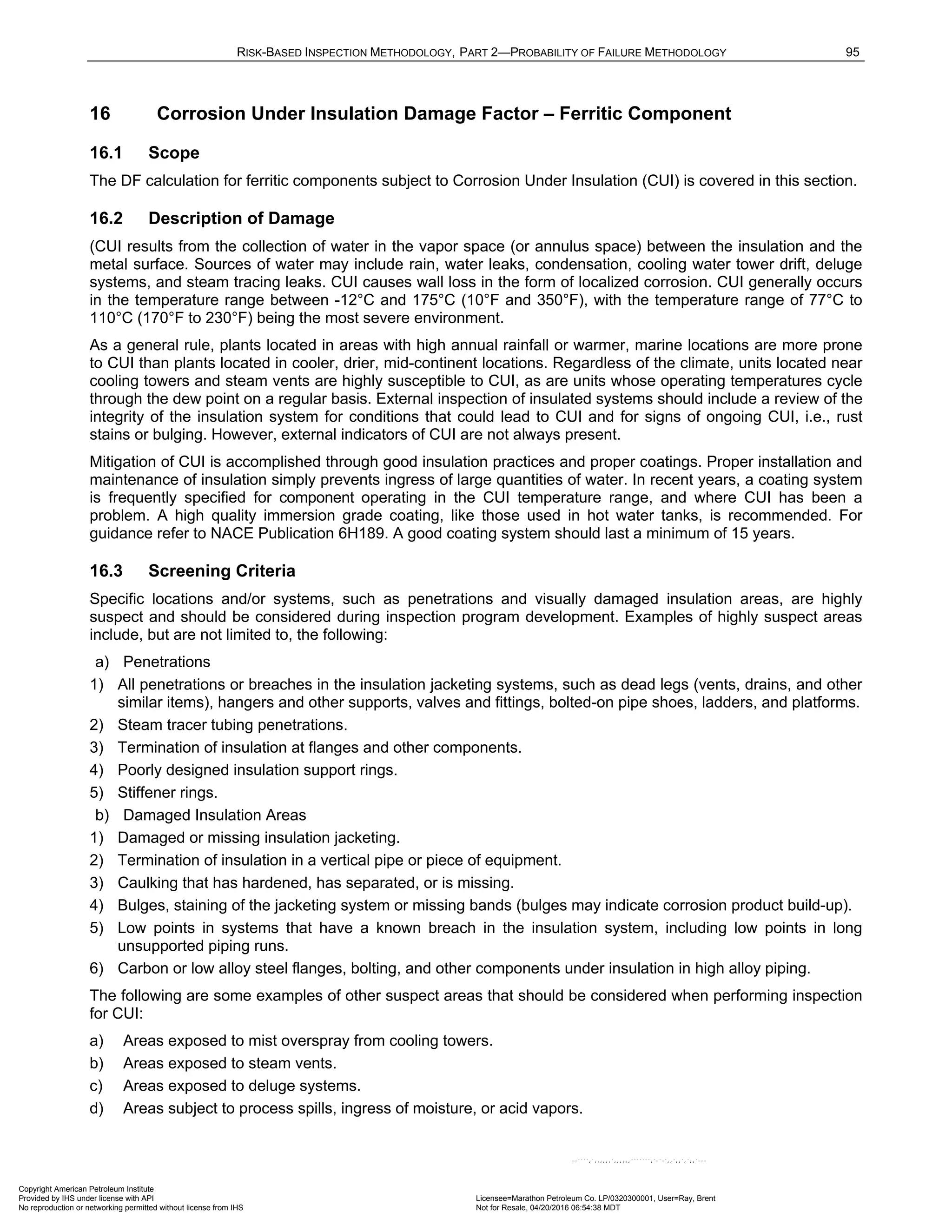
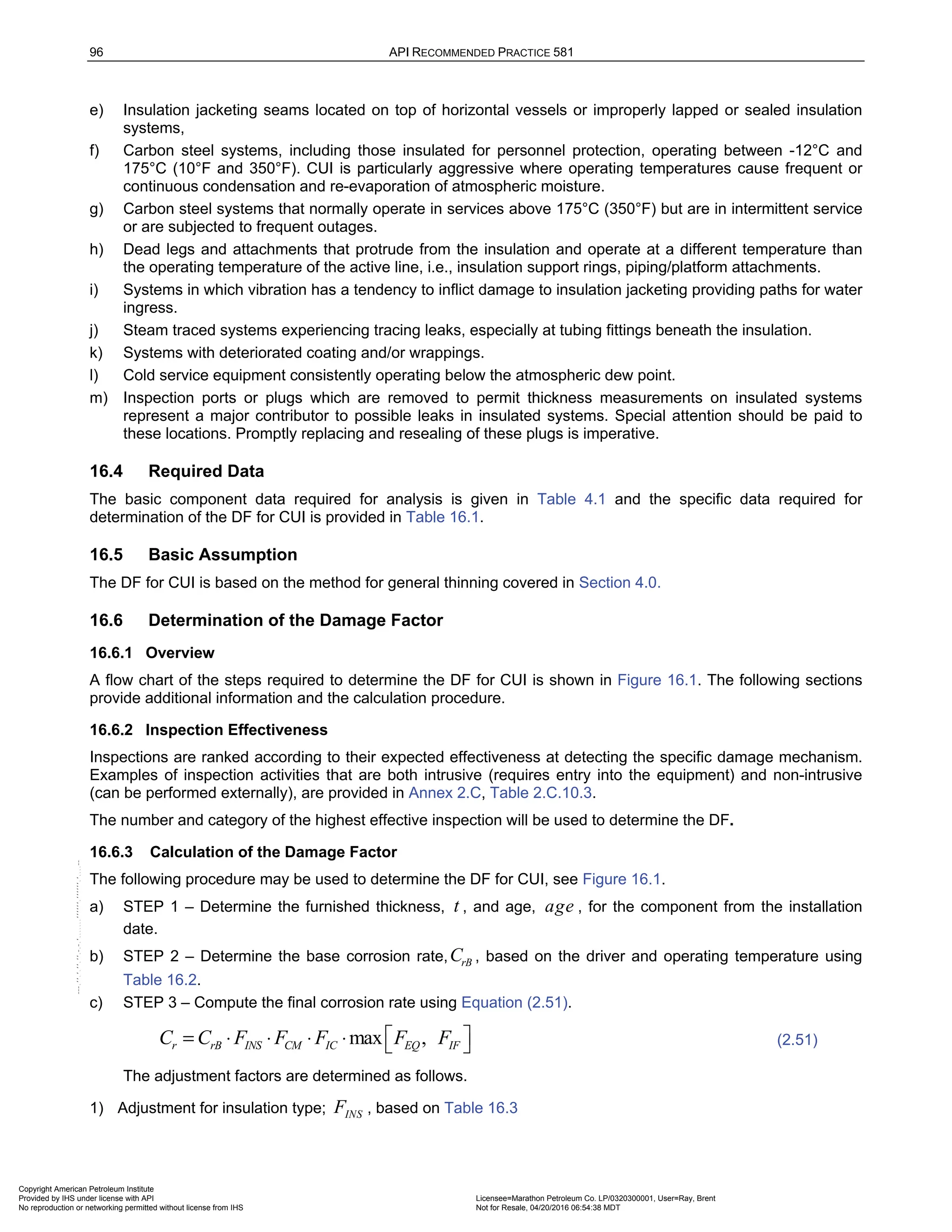
![RISK-BASED INSPECTION METHODOLOGY, PART 2—PROBABILITY OF FAILURE METHODOLOGY 97
2) Adjustment for Complexity, CM
F – Established based on the following criteria.
• If the complexity is below average, then 0.75
CM
F = .
• If the complexity is average, then 1.0
CM
F = .
• If the complexity is above average, then 1.25
CM
F = .
3) Adjustment for Insulation Condition, IC
F – Established based on the following criteria.
• If the insulation condition is below average, then 1.25
IC
F = .
• If the insulation condition is average, then 1.0
IC
F = .
• If the insulation condition is above average, then 0.75
IC
F = .
4) Adjustment for Equipment Design or Fabrication, EQ
F – If equipment has a design which allows water to
pool and increase metal loss rates, such as piping supported directly on beams, vessel external stiffening
rings or insulation supports or other such configuration that does not allow water egress and/or does not
allow for proper coating maintenance, then 2
EQ
F = ; otherwise, 1
EQ
F = .
5) Adjustment for Interface, IF
F – If the piping has an interface where it enters either soil or water, then
2
IF
F = ; otherwise, 1
IF
F = .
d) STEP 4 – Determine the time in-service, tk
age , since the last known thickness, rde
t (see Section 4.5.5).
The rde
t is the starting thickness with respect to wall loss associated with external corrosion (see Section
4.5.5). If no measured thickness is available, set rde
t t
= and tk
age age
= .
e) STEP 5 – Determine the in-service time, coat
age , since the coating has been installed using Equation
(2.52).
coat
age Calculation Date Coating Installation Date
= − (2.52)
f) STEP 6 – Determine the coating adjustment, adj
Coat , using Equations (2.53) through (2.58).
If :
tk coat
age age
≥
0
adj
Coat No Coating or Poor Coating Quality
=
(2.53)
[ ]
min 5,
adj coat
Coat age Medium Coating Quality
= (2.54)
[ ]
min 15,
adj coat
Coat age High Coating Quality
= (2.55)
If :
tk coat
age age
<
0
adj
Coat No Coating or Poor Coating Quality
=
(2.56)
[ ] [ ]
min 5, min 5,
adj coat coat tk
Coat age age age Medium Coating Quality
= − − (2.57)
[ ] [ ]
min 15, min 15,
adj coat coat tk
Coat age age age High Coating Quality
= − − (2.58)
g) STEP 7 – Determine the in-service time, age , over which CUI may have occurred using Equation (2.59).
tk adj
age age Coat
= − (2.59)
Copyright American Petroleum Institute
Provided by IHS under license with API Licensee=Marathon Petroleum Co. LP/0320300001, User=Ray, Brent
Not for Resale, 04/20/2016 06:54:38 MDT
No reproduction or networking permitted without license from IHS
--````,`,,,,,,`,,,,,,```````,`-`-`,,`,,`,`,,`---](https://image.slidesharecdn.com/api581-3rdedition-april2016-240227010601-3bf73ab5/75/Norma-API-581-3rd-Edition-April-2016-pdf-230-2048.jpg)
![98 API RECOMMENDED PRACTICE 581
h) STEP 8 – Determine the allowable stress, S , weld joint efficiency, E , and minimum required thickness,
min
t , per the original construction code or API 579-1/ASME FFS-1 [10]. In cases where components are
constructed of uncommon shapes or where the component's minimum structural thickness, c
t , may govern,
the user may use the c
t in lieu of min
t where pressure does not govern the minimum required thickness
criteria.
i) STEP 9 - Determine the rt
A parameter using Equation (2.60) based on the age and rde
t from STEP 4,
r
C from STEP 3.
r
rt
rde
C age
A
t
⋅
= (2.60)
j) STEP 10 – Calculate the Flow Stress, CUIF
FS , using E from STEP 8 and Equation (2.61).
( ) 1.1
2
CUIF YS TS
FS E
+
== ⋅ ⋅ (2.61)
Note: Use Flow Stress ( Thin
FS ) at design temperature for conservative results, using the appropriate
Equation (2.62) or (2.63).
k) STEP 11 – Calculate strength ratio parameter, Thin
P
SR , using Equation (2.62) or (2.63).
1) Use Equation (2.62) with rde
t from STEP 4 and S , E and min
t or c
t from STEP 8 and flow stress CUIF
FS
from STEP 10.
min
( , )
CUIF c
P CUIF
rde
S E Min t t
SR
FS t
⋅
= ⋅ (2.62)
Note: The min
t is based on a design calculation that includes evaluation for internal pressure hoop
stress, external pressure and/or structural considerations, as appropriate. The minimum required
thickness calculation is the design code min
t . Consideration for internal pressure hoop stress alone
may not be sufficient. c
t as defined in STEP 5 may be used when appropriate.
Use Equation (2.63) with rde
t from STEP 3 and flow stress CUIF
FS from STEP 10.
CUIF
P CUIF
rde
P D
SR
FS t
α
⋅
=
⋅ ⋅
(2.63)
Where α is the shape factor for the component type
2 ,4 ,1.13
for a cylinder for a sphere for a head
α = .
Note: This strength ratio parameter is based on internal pressure hoop stress only. It is not
appropriate where external pressure and/or structural considerations dominate. . When c
t dominates
or if the min
t is calculated using another method, Equation (2.62) should be used.
l) STEP 12 – Determine the number of inspections, C U IF
A
N , C U IF
B
N , C U IF
C
N , C U IF
D
N , and the corresponding
inspection effectiveness category using Section 16.6.2 for all past inspections.
Copyright American Petroleum Institute
Provided by IHS under license with API Licensee=Marathon Petroleum Co. LP/0320300001, User=Ray, Brent
Not for Resale, 04/20/2016 06:54:38 MDT
No reproduction or networking permitted without license from IHS
--````,`,,,,,,`,,,,,,```````,`-`-`,,`,,`,`,,`---](https://image.slidesharecdn.com/api581-3rdedition-april2016-240227010601-3bf73ab5/75/Norma-API-581-3rd-Edition-April-2016-pdf-231-2048.jpg)
![RISK-BASED INSPECTION METHODOLOGY, PART 2—PROBABILITY OF FAILURE METHODOLOGY 99
m) STEP 13 – Determine the inspection effectiveness factors, 1
CUIF
I , 2
CUIF
I , 3
CUIF
I , using Equation (2.64),
Prior Probabilities, 1
CUIF
p
Pr , 2
CUIF
p
Pr and 3
CUIF
p
Pr , from Table 5.6, Conditional Probabilities (for each
inspection effectiveness level), 1
CUIF
p
Co , 2
CUIF
p
Co and 3
CUIF
p
Co , from Table 5.7, and the number of
inspections, C U IF
A
N , C U IF
B
N , C U IF
C
N , C U IF
D
N , in each effectiveness level obtained from STEP 12.
( ) ( ) ( ) ( )
( ) ( ) ( ) ( )
( ) ( )
1 1 1 1 1 1
2 2 2 2 2 2
3 3 3 3 3
CUIF CUIF CUIF CUIF
A B C D
CUIF CUIF CUIF CUIF
A B C D
CUIF CUIF
A B
N N N N
CUIF CUIF CUIFA CUIFB CUIFC CUIFD
p p p p p
N N N N
CUIF CUIF CUIFA CUIFB CUIFC CUIFD
p p p p p
N N
CUIF CUIF CUIFA CUIFB C
p p p p
I Pr Co Co Co Co
I Pr Co Co Co Co
I Pr Co Co Co
=
=
= ( ) ( )
3
CUIF CUIF
C D
N N
UIFC CUIFD
p
Co
(2.64)
s) STEP 14 – Calculate the Posterior Probabilities, 1
CUIF
p
Po , 2
CUIF
p
Po and 3
CUIF
p
Po using Equation (2.65) with
1
CUIF
I , 2
CUIF
I and 3
CUIF
I in Step 13.
1
1
1 2 3
2
2
1 2 3
3
3
1 2 3
CUIF
CUIF
p CUIF CUIF CUIF
CUIF
CUIF
p CUIF CUIF CUIF
CUIF
CUIF
p CUIF CUIF CUIF
I
Po
I I I
I
Po
I I I
I
Po
I I I
=
+ +
=
+ +
=
+ +
(2.65)
t) STEP 15 – Calculate the parameters, 1 2 3
, ,
CUIF CUIF CUIF
β β β using Equation (2.66) and assigning
0.20
t
COVΔ = , 0.20
f
S
COV = and 0.05
P
COV = .
( )
( )
1
1 1
2
2 2
3
3 3
1 2
2 2 2 2 2 2
2 2
2 2 2 2 2 2
3
2 2 2
1
,
1 ( )
1
,
1 ( )
1
1
f
f
CUIF
S rt p
CUIF
CUIF
S rt t S rt S p P
CUIF
S rt p
CUIF
CUIF
S rt t S rt S p P
CUIF
S rt p
CUIF
S rt t S
D A SR
D A COV D A COV SR COV
D A SR
D A COV D A COV SR COV
D A SR
D A COV D A
β
β
β
Δ
Δ
Δ
− ⋅ −
=
⋅ ⋅ + − ⋅ ⋅ + ⋅
− ⋅ −
=
⋅ ⋅ + − ⋅ ⋅ + ⋅
− ⋅ −
=
⋅ ⋅ + − ⋅
( )
2
2 2 2
.
( )
f
CUIF
rt S p P
COV SR COV
⋅ + ⋅
(2.66)
Where 1
1
S
D = , 2
2
S
D = and 3
4
S
D = . These are the corrosion rate factors for damage states 1, 2 and 3 as
as discussed in 4.5.3 [35]. Note that the DF calculation is very sensitive to the value used for the coefficient
of variance for thickness, t
COVΔ . The t
COVΔ is in the range 0.10 0.20
t
COVΔ
≤ ≤ , with a
recommended conservative value of 0.20
t
COVΔ = .
Copyright American Petroleum Institute
Provided by IHS under license with API Licensee=Marathon Petroleum Co. LP/0320300001, User=Ray, Brent
Not for Resale, 04/20/2016 06:54:38 MDT
No reproduction or networking permitted without license from IHS
--````,`,,,,,,`,,,,,,```````,`-`-`,,`,,`,`,,`---](https://image.slidesharecdn.com/api581-3rdedition-april2016-240227010601-3bf73ab5/75/Norma-API-581-3rd-Edition-April-2016-pdf-232-2048.jpg)
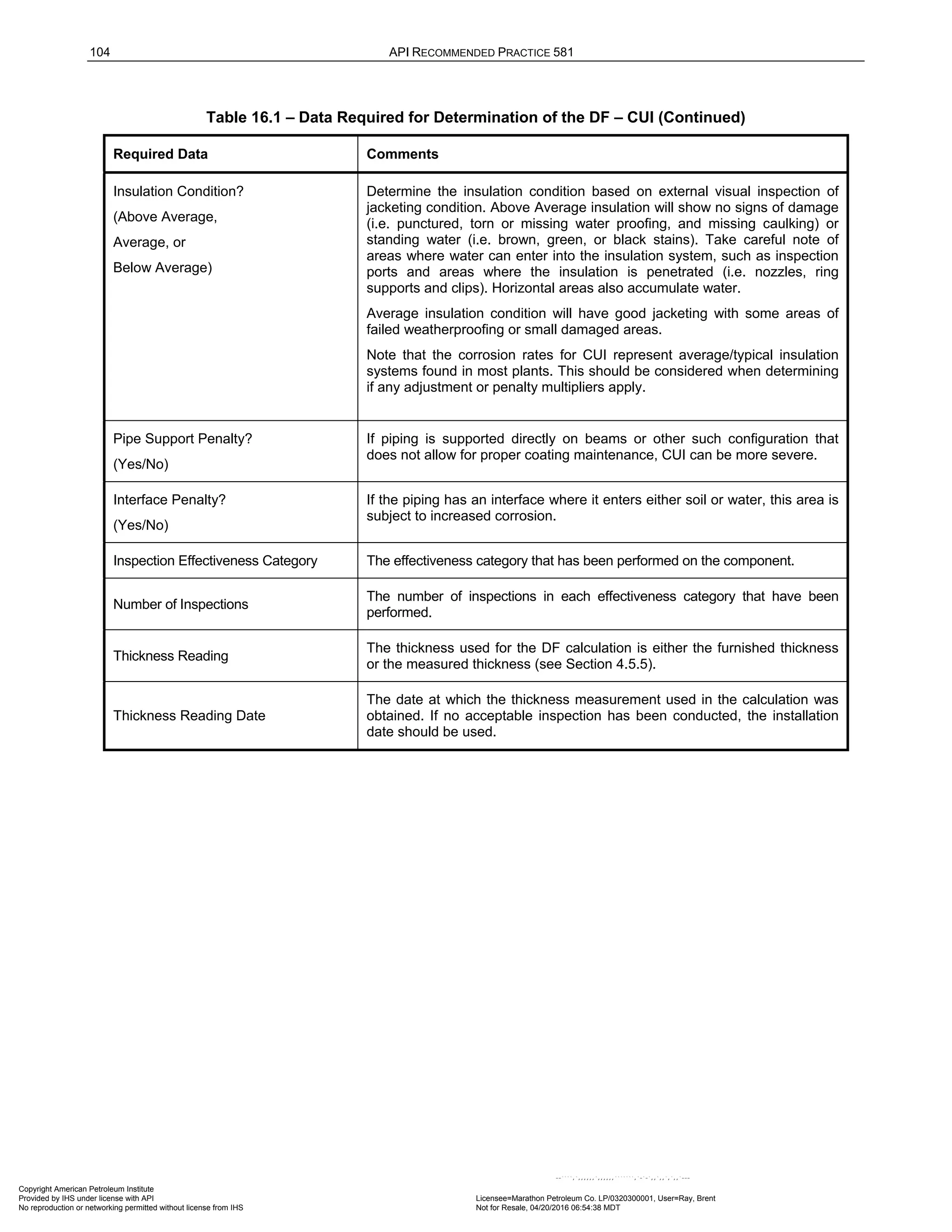
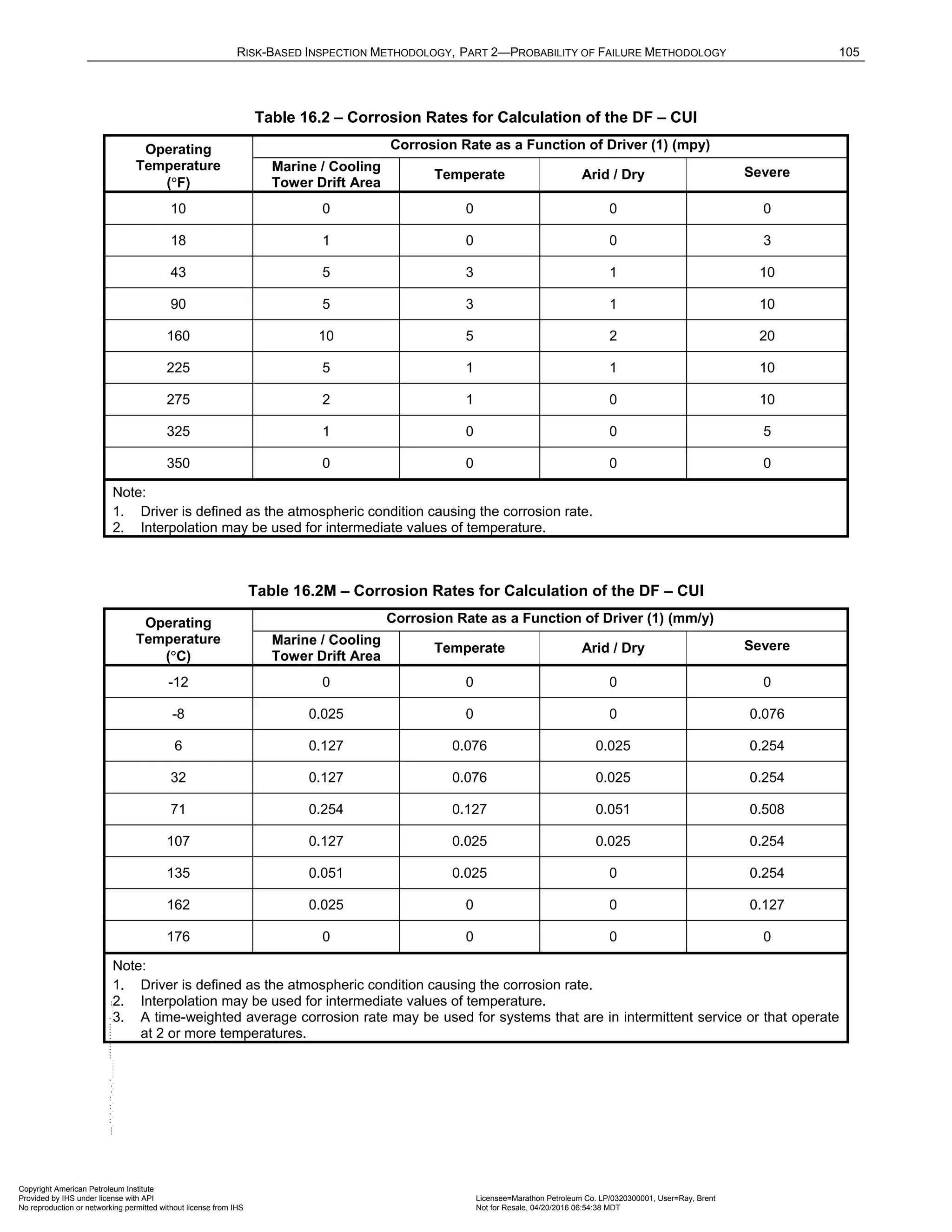
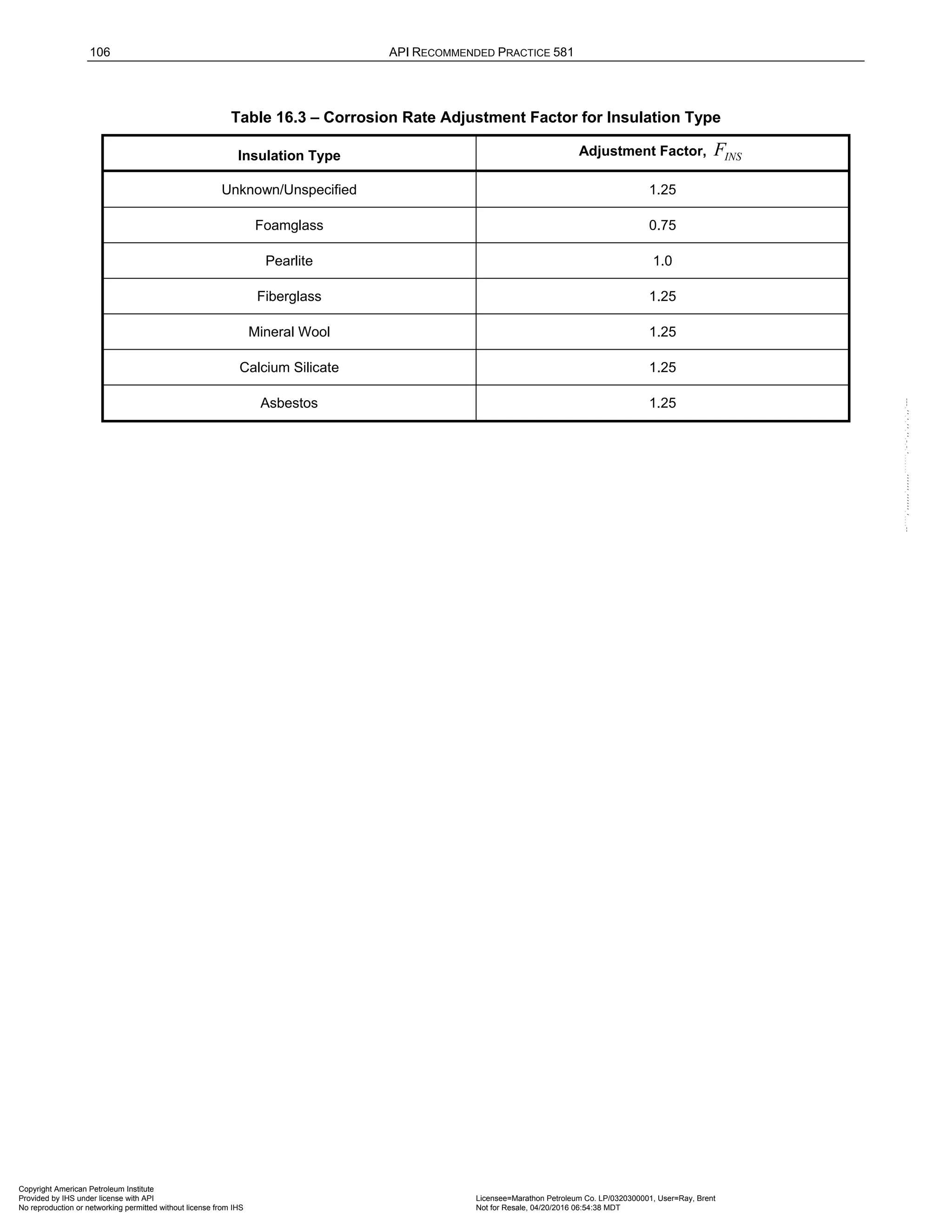
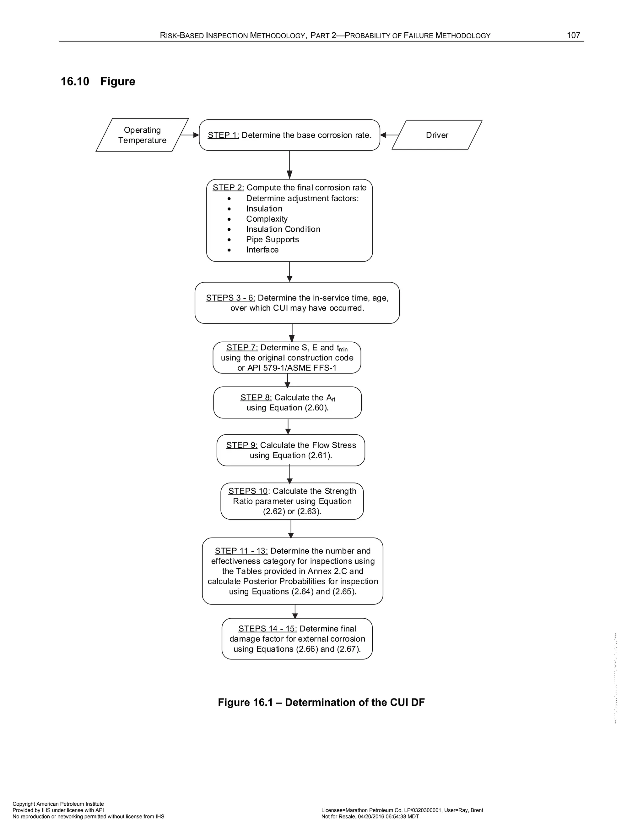
![RISK-BASED INSPECTION METHODOLOGY, PART 2—PROBABILITY OF FAILURE METHODOLOGY 109
17.6.3 Calculation of the Damage Factor
The following procedure may be used to determine the DF for external CLSCC, see Figure 17.1.
a) STEP 1 – Determine the susceptibility using Table 17.2 based on the driver and the operating temperature.
Note that a HIGH susceptibility should be used if cracking is confirmed to be present.
b) STEP 2 – Determine the Severity Index, VI
S , using Table 17.3 based on the susceptibility from STEP 1.
c) STEP 3 – Determine the in-service time, crack
age , over which external CLSCC. If no acceptable
inspections have been performed, the time in-service since installation should be used.
d) STEP 4 – Determine the in-service time, coat
age , since the coating has been installed using Equation
(2.68)
coat
age Calculation Date Coating Installation Date
= − (2.68)
e) STEP 5 – Determine the coating adjustment, adj
Coat , using Equations (2.69) through (2.74).
If :
crack coat
age age
≥
0
adj
Coat No Coating or Poor Coating Quality
=
(2.69)
[ ]
min 5,
adj coat
Coat age Medium Coating Quality
= (2.70)
[ ]
min 15,
adj coat
Coat age High Coating Quality
= (2.71)
If :
crack coat
age age
<
0
adj
Coat No Coating or Poor Coating Quality
=
(2.72)
[ ] [ ]
min 5, min 5,
adj coat coat crack
Coat age age age Medium Coating Quality
= − − (2.73)
[ ] [ ]
min 15, min 15,
adj coat coat crack
Coat age age age High Coating Quality
= − − (2.74)
f) STEP 6 – Determine the in-service time, age , over which external CLSCC may have occurred using
Equation (2.75).
crack adj
age age Coat
= − (2.75)
g) STEP 7 – Determine the number of inspections performed with no cracking detected or cracking was
repaired, and the corresponding inspection effectiveness category using Section 17.6.2 for past inspections
performed during the in-service time. Combine the inspections to the highest effectiveness performed using
Section 3.4.3. Cracking detected but not repaired should be evaluated and future inspection
recommendations based upon FFS evaluation.
h) STEP 8 – Determine the base DF for external CLSCC,
ext CLSCC
fB
D −
, using Table 6.3 based on the number
of, and the highest inspection effectiveness determined in STEP 7, and the severity index, VI
S , from STEP
2.
i) STEP 9 – Calculate the escalation in the DF based on the time in-service since the last inspection using
the age from STEP 6 and Equation (2.76). In this equation, it is assumed that the probability for cracking
will increase with time since the last inspection as a result of increased exposure to upset conditions and
other non-normal conditions.
Copyright American Petroleum Institute
Provided by IHS under license with API Licensee=Marathon Petroleum Co. LP/0320300001, User=Ray, Brent
Not for Resale, 04/20/2016 06:54:38 MDT
No reproduction or networking permitted without license from IHS
--````,`,,,,,,`,,,,,,```````,`-`-`,,`,,`,`,,`---](https://image.slidesharecdn.com/api581-3rdedition-april2016-240227010601-3bf73ab5/75/Norma-API-581-3rd-Edition-April-2016-pdf-242-2048.jpg)
![110 API RECOMMENDED PRACTICE 581
( )
1.1
[ ,1.0]
ext CLSCC ext CLSCC
f fB
D D Max age
− −
= ⋅ (2.76)
17.7 Nomenclature
age is the component in-service time since the last cracking inspection or service start date
coat
age is the in-service time since the coating installation
crack
age is the in-service time since the last CLSCC inspection
adj
Coat is the coating adjustment
ext CLSCC
f
D −
is the DF for external CLSCC
ext CLSCC
fB
D −
is the base value of the DF for external CLSCC
VI
S is the severity index
17.8 Tables
Table 17.1 – Data Required for Determination of the Damage Factor – External CLSCC
Required Data Comments
Driver The drivers for external CLSCC. This can be the weather at a
location (e.g., marine), the potential for cooling tower drift, the use of
sprinkler systems, or other contributors.
Crack Severity Crack severity based on susceptibility (Temperature, and Weather,
see below).
Date The date the component was installed or the date of the last
inspection where no damage was found
Coating Quality Relates to the type of coating applied, for example:
None – No coating or primer only.
Medium – Single coat epoxy.
High – Multi coat epoxy or filled epoxy.
Coating Date Determine the age of the coating.
Inspection Effectiveness Category
The effectiveness category that has been performed on the
component.
Number of Inspections
The number of inspections in each effectiveness category that have
been performed.
Operating Temperature, °C (°F) Determine the expected operating temperature (consider normal and
non-normal operating conditions).
Copyright American Petroleum Institute
Provided by IHS under license with API Licensee=Marathon Petroleum Co. LP/0320300001, User=Ray, Brent
Not for Resale, 04/20/2016 06:54:38 MDT
No reproduction or networking permitted without license from IHS
--````,`,,,,,,`,,,,,,```````,`-`-`,,`,,`,`,,`---](https://image.slidesharecdn.com/api581-3rdedition-april2016-240227010601-3bf73ab5/75/Norma-API-581-3rd-Edition-April-2016-pdf-243-2048.jpg)
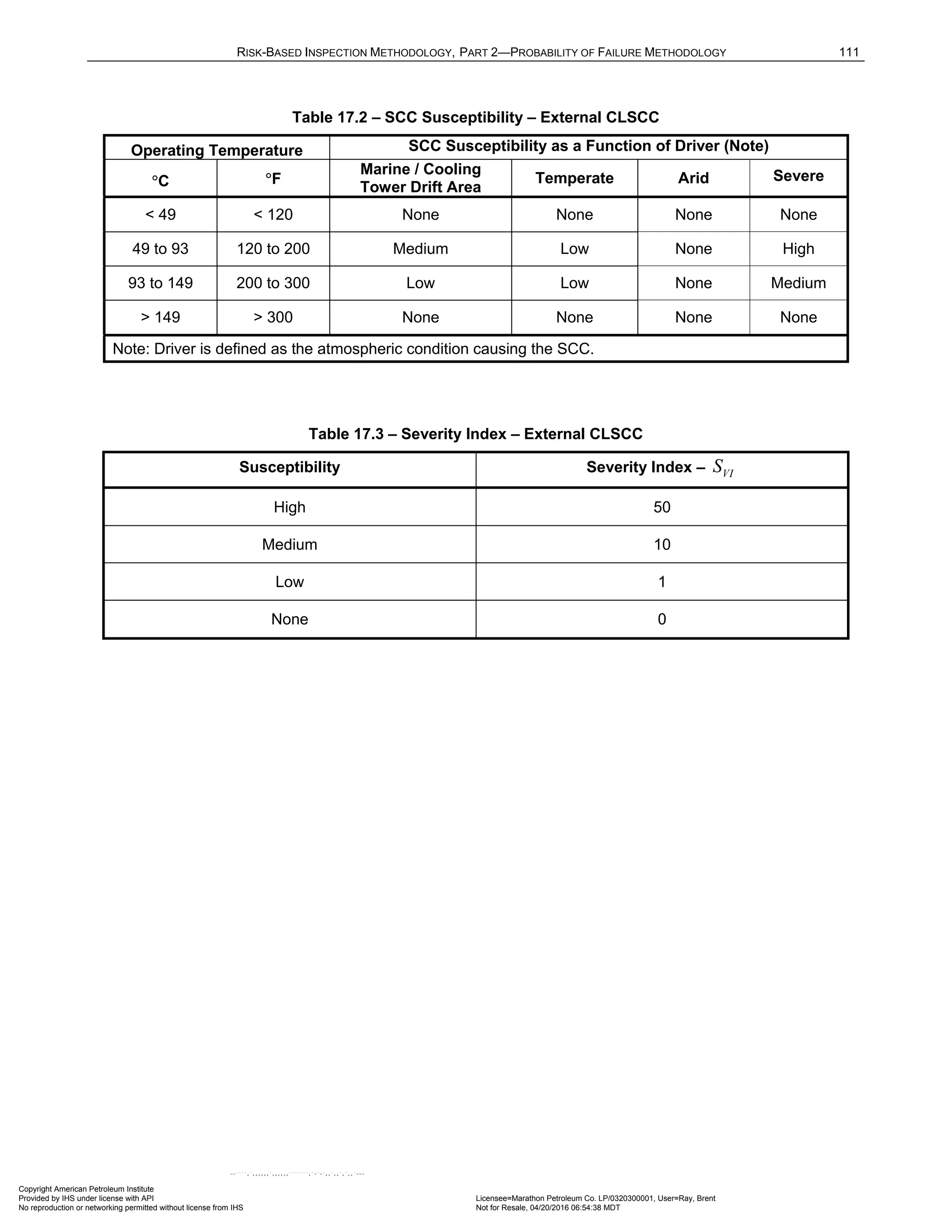
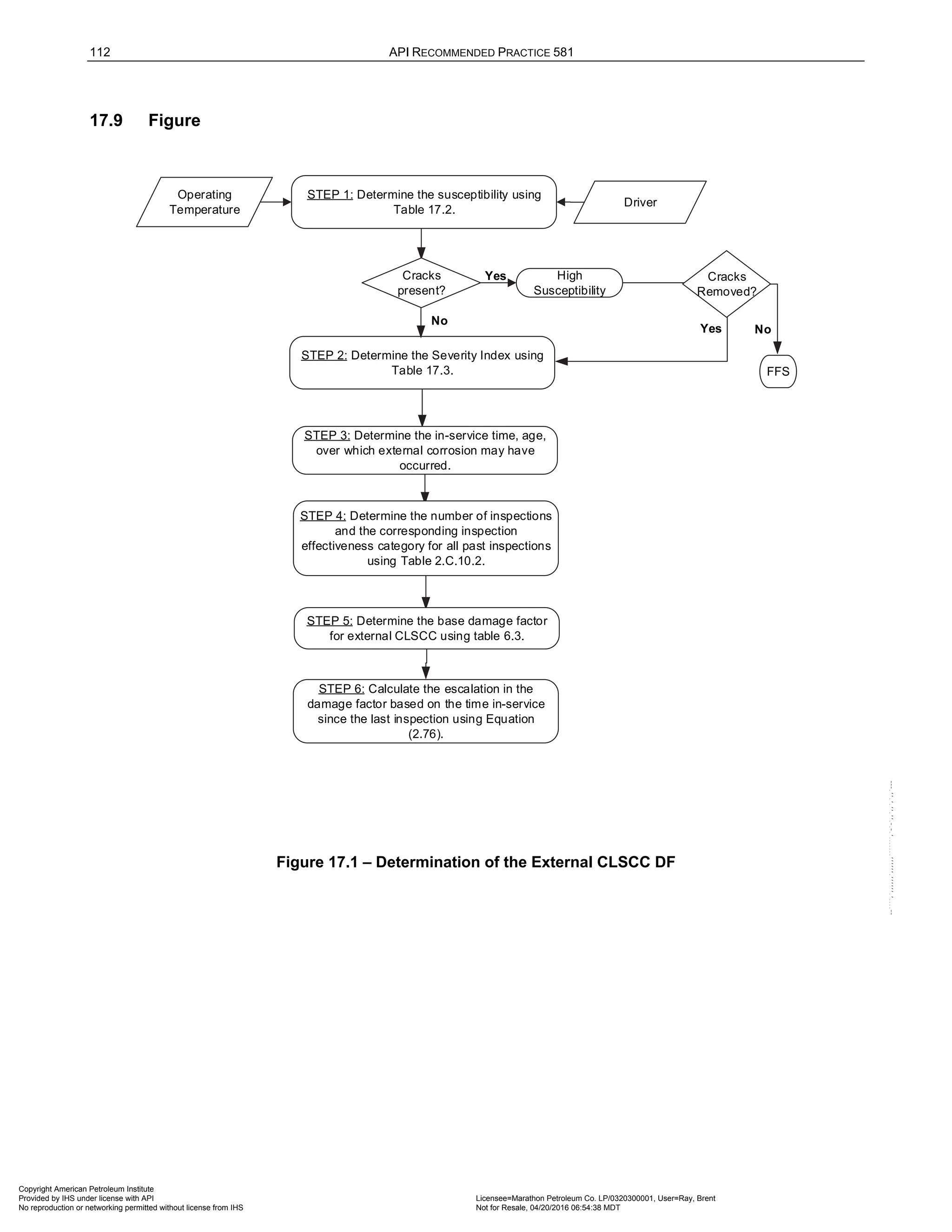
![114 API RECOMMENDED PRACTICE 581
18.6.2 Inspection Effectiveness
Inspections are ranked according to their expected effectiveness at detecting the specific damage mechanism.
Examples of inspection activities that are both intrusive (requires entry into the equipment) and non-intrusive
(can be performed externally), are provided in Annex 2.C, Table 2.C.10.4.
If multiple inspections of a lower effectiveness have been conducted during the designated time period, they can
be equated to an equivalent higher effectiveness inspection in accordance with Section 3.4.3.
18.6.3 Calculation of the Damage Factor
The following procedure may be used to determine the DF for CUI CLSCC, see Figure 18.1. Note that a HIGH
susceptibility should be used if cracking is known to be present.
a) STEP 1 – Determine the susceptibility using Table 18.2 based on the driver and the operating temperature
and the following adjustment factors.
1) Adjustments for Piping Complexity – If the piping complexity is Below Average, then decrease Susceptibility
one level (e.g. Medium to Low). If the piping complexity is Above Average, then increase Susceptibility one
level (e.g., Medium to High). If the piping complexity is Average, then there is no change in the
susceptibility.
2) Adjustments for Insulation Condition – If the insulation condition is Above Average, then decrease
Susceptibility one level (e.g., Medium to Low). If the insulation condition is Below Average, then increase
Susceptibility one level (e.g., Medium to High). If the insulation condition is Average, then there is no change
in the susceptibility.
3) Adjustments for Chloride Free Insulation – If the insulation contains chlorides, then there is no change in the
susceptibility. If the insulation is chloride free, then decrease the Susceptibility one level (e.g., Medium to
Low).
Note that a High susceptibility should be used if cracking is confirmed to be present.
b) STEP 2 – Determine the Severity Index, VI
S , using Table 17.3, based on the susceptibility from STEP 1.
c) STEP 3 – Determine the in-service time, crack
age , since the last inspection. If no acceptable inspections
have been performed, the time in-service since installation should be used.
d) STEP 4 – Determine the in-service time, coat
age , since the coating has been installed using Equation
(2.77).
age Calculation Date Coating Installation Date
= − (2.77)
e) STEP 5 – Determine the coating adjustment, , using Equations (2.78) through (2.83).
If :
crack coat
age age
≥
0
adj
Coat No Coating or Poor Coating Quality
=
(2.78)
[ ]
min 5,
adj coat
Coat age Medium Coating Quality
= (2.79)
[ ]
min 15,
adj coat
Coat age High Coating Quality
= (2.80)
If :
crack coat
age age
<
0
adj
Coat No Coating or Poor Coating Quality
=
(2.81)
[ ] [ ]
min 5, min 5,
adj coat coat crack
Coat age age age Medium Coating Quality
= − − (2.82)
(2.83)
[ ] [ ]
min 15, min 15,
adj coat coat crack
Coat age age age High Coating Quality
= − −
Copyright American Petroleum Institute
Provided by IHS under license with API Licensee=Marathon Petroleum Co. LP/0320300001, User=Ray, Brent
Not for Resale, 04/20/2016 06:54:38 MDT
No reproduction or networking permitted without license from IHS
--````,`,,,,,,`,,,,,,```````,`-`-`,,`,,`,`,,`---](https://image.slidesharecdn.com/api581-3rdedition-april2016-240227010601-3bf73ab5/75/Norma-API-581-3rd-Edition-April-2016-pdf-247-2048.jpg)
![RISK-BASED INSPECTION METHODOLOGY, PART 2—PROBABILITY OF FAILURE METHODOLOGY 115
f) STEP 5 – Determine the in-service time, age , over which external CUI CLSCC may have occurred using
Equation (2.84).
crack adj
age age Coat
= − (2.82)
g) STEP 6 – Determine the number of inspections performed with no cracking detected or cracking was
repaired, and the corresponding inspection effectiveness category using Section 18.6.2 for past inspections
performed during the in-service time. Combine the inspections to the highest effectiveness performed using
Section 3.4.3. Cracking detected but not repaired should be evaluated and future inspection
recommendations based upon FFS evaluation
h) STEP 8 – Determine the base DF for CUI CLSCC,
CUI CLSCC
fB
D −
, using Table 6.3 based on the number of,
and the highest inspection effectiveness determined in STEP 6, and the severity index, VI
S , from STEP 2.
i) STEP 9 – Calculate the escalation in the DF based on the time in-service since the last inspection using
the age from STEP 6 and Equation (2.85). In this equation, it is assumed that the probability for cracking
will increase with time since the last inspection as a result of increased exposure to upset conditions and
other non-normal conditions.
( )
1.1
[ ,1.0]
CUI CLSCC CUI CLSCC
f fB
D D Max age
− −
= ⋅ (2.85)
18.7 Nomenclature
age is the component in-service time since the last cracking inspection or service start date
coat
age is the in-service time since the coating installation
crack
age is the in-service time since the last CLSCC inspection
adj
Coat is the coating adjustment
CUI CLSCC
f
D −
is the DF for CUI CLSCC
CUI CLSCC
fB
D −
is the base value of the DF for CUI CLSCC
VI
S is the severity index
18.8 References
1. API Recommended Practice 583 Corrosion Under Insulation and Fireproofing, American Petroleum
Institute, Washington, D.C, 20005.
Copyright American Petroleum Institute
Provided by IHS under license with API Licensee=Marathon Petroleum Co. LP/0320300001, User=Ray, Brent
Not for Resale, 04/20/2016 06:54:38 MDT
No reproduction or networking permitted without license from IHS
--````,`,,,,,,`,,,,,,```````,`-`-`,,`,,`,`,,`---](https://image.slidesharecdn.com/api581-3rdedition-april2016-240227010601-3bf73ab5/75/Norma-API-581-3rd-Edition-April-2016-pdf-248-2048.jpg)
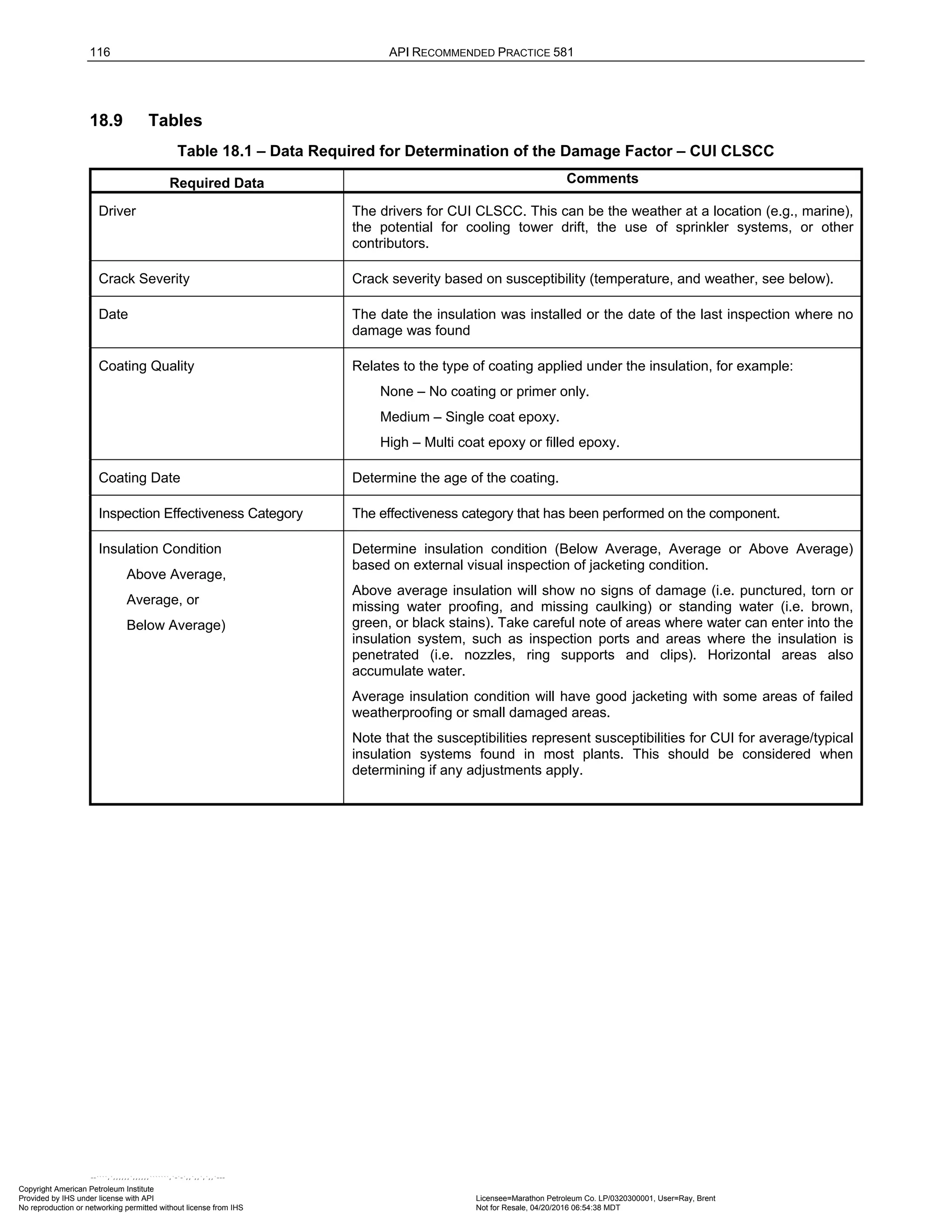
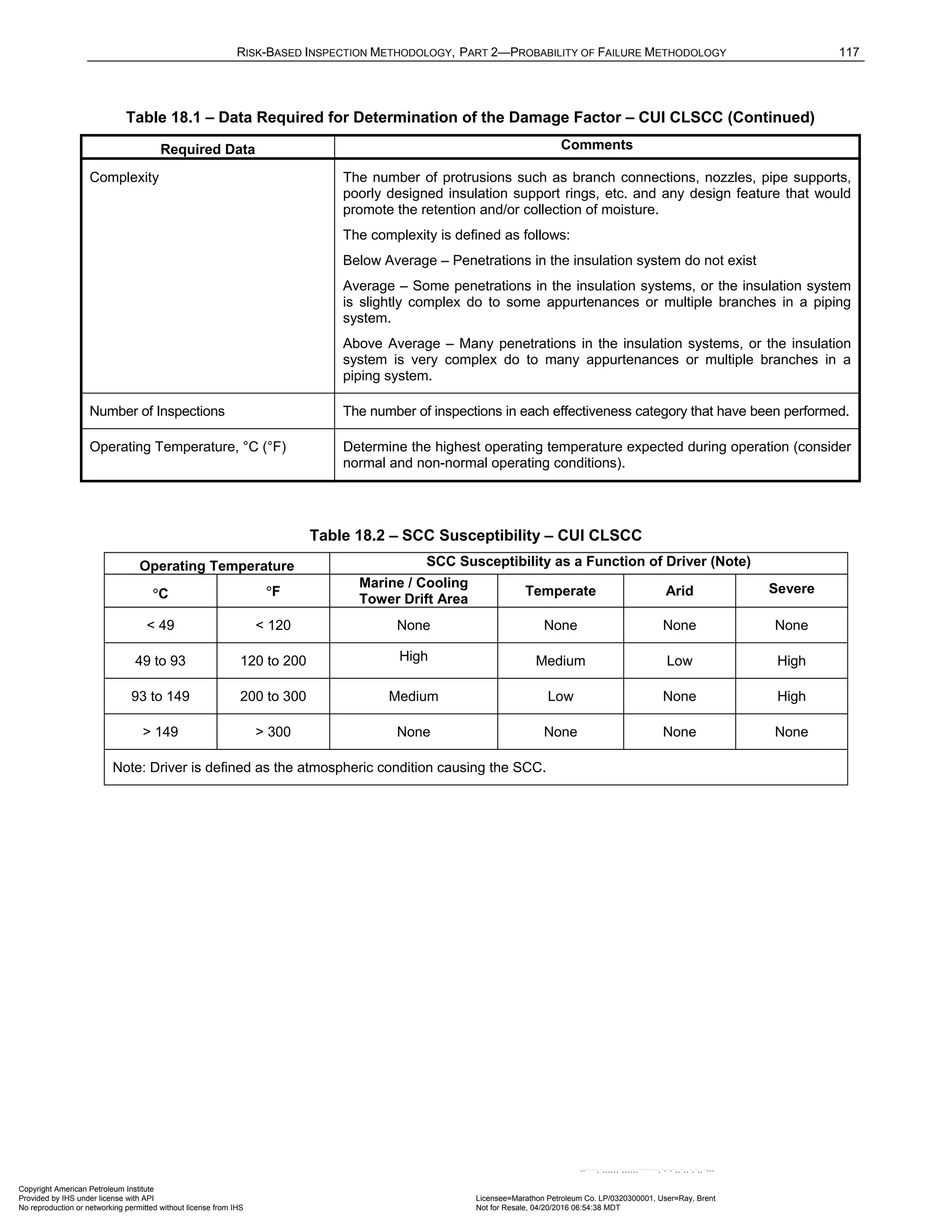
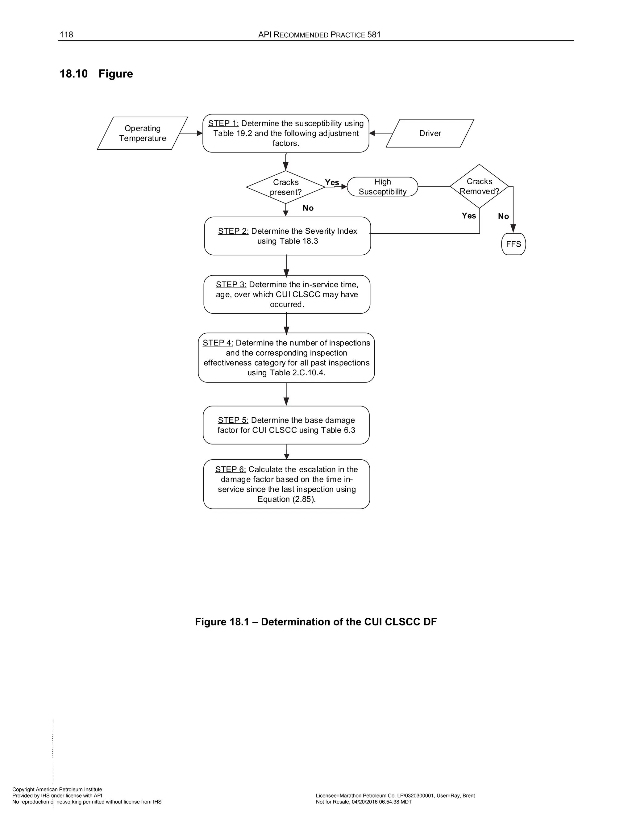
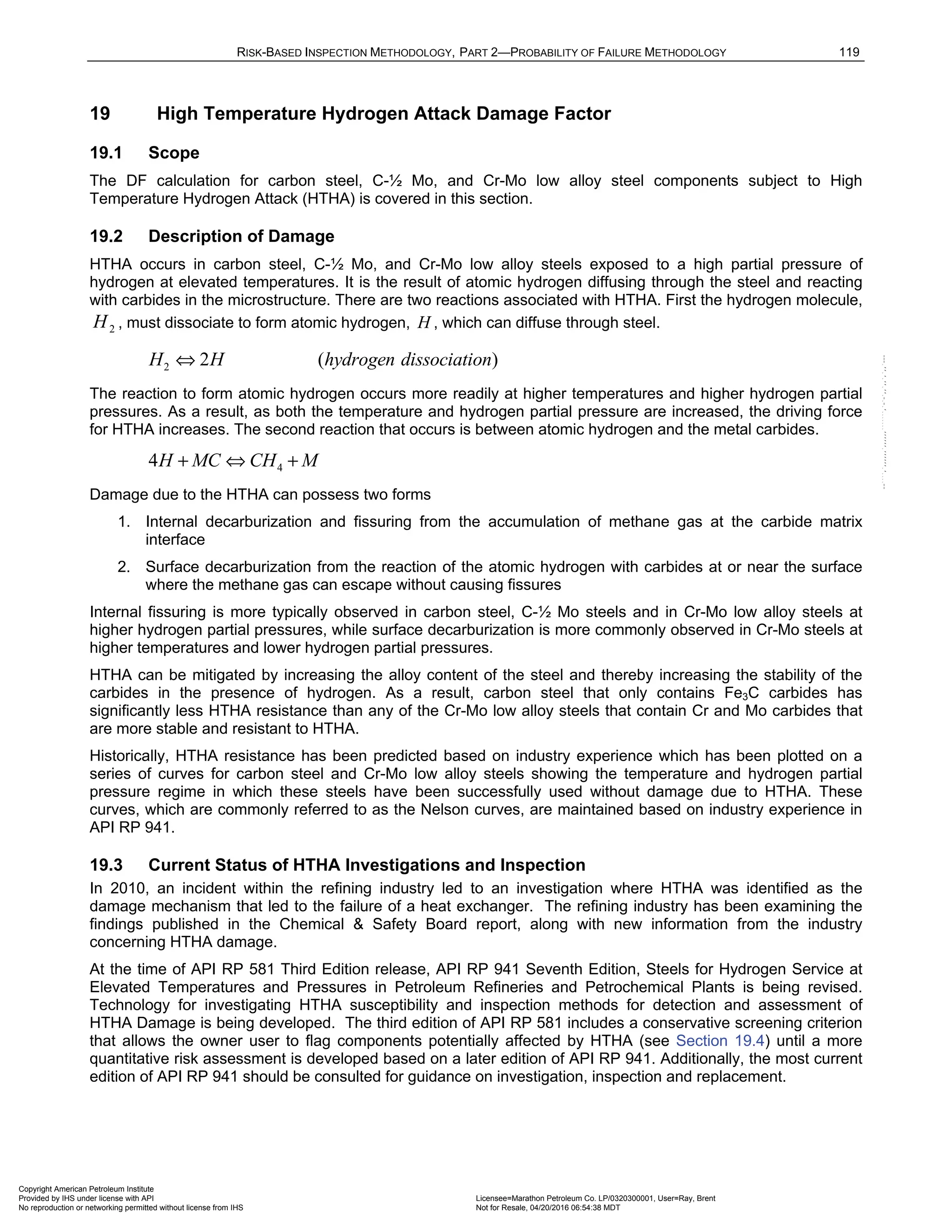
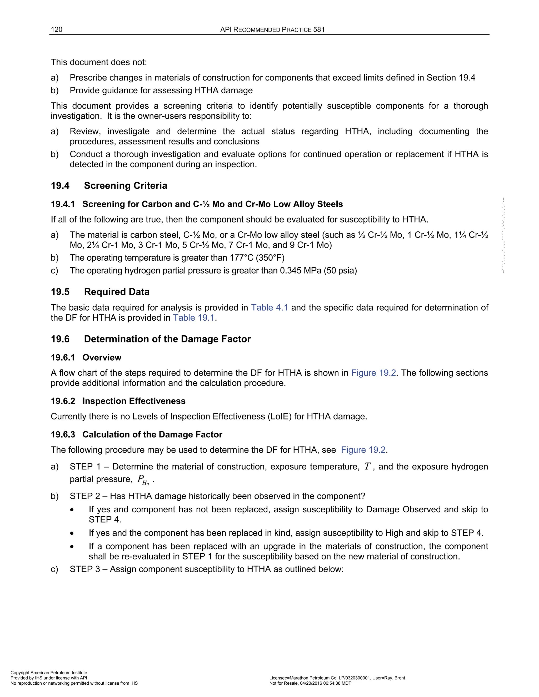
![RISK-BASED INSPECTION METHODOLOGY, PART 2—PROBABILITY OF FAILURE METHODOLOGY 121
1) For Carbon and C-½ Mo Alloy Steels:
a) If the exposure temperature is > 177°C (350°F) and the exposure hydrogen partial pressure is >
0.345 MPa (50 psia), assign a High susceptibility to HTHA.
b) If exposure temperature is < 177°C (350°F) and the exposure hydrogen partial pressure is < 0.345
MPa (50 psia), assign HTHA susceptibility to None.
2) For all other Cr-Mo Low Alloy Steels
a) If the exposure temperature is >177°C (> 350°F) and exposure hydrogen partial pressure is >0.345
MPa (> 50 psia) calculate T
Δ proximity to the API 941 curve usingT and 2
H
P from STEP 1. Assign
HTHA susceptibility using Figure 19.1.
Note that the approach used in Figure 19.1 is an example guideline using 27.7°C (50°F) increments. The
27.7°C (50°F) increments were used to represent relative changes in susceptibility. It is the owner-user’s
responsibility to customize the values to represent their practice for determining HTHA susceptibility.
d) STEP 4 – Determine the DF for HTHA,
HTHA
f
D , using Table 19.2 based on the susceptibility from STEP 2
or STEP 3.
19.6.4 Consideration of Susceptibility
The time in service of component significantly affects susceptibility to HTHA and should be considered during
the HTHA review. Additionally, steels fabricated prior to 1970 may contain impurities and/or inclusions that were
introduced during fabrication. As these steels age, they may become more susceptible to HTHA for similar
process conditions compared to steels fabricated in 1980 or later. As a result, the owner-user may choose more
conservative guidelines by increasing the susceptibilities in Table 19.2.
19.7 Nomenclature
HTHA
f
D is the DF for HTHA
2
H
P is the hydrogen partial pressure, MPa [psia]
T is the operating temperature, °C [°F]
19.8 Tables
Table 19.1 – Data Required for Determination of Susceptibility to HTHA
Required Data Comments
Material of Construction The component generic construction material (e.g. carbon steel, C-½ Mo, 2 ¼
Cr-1 Mo).
Hydrogen Partial Pressure,
MPa (psia)
Determine the hydrogen partial pressure, which is equal to the product of the mole
fraction of hydrogen and the total pressure (absolute).
Temperature, °C (°F) The temperature of exposure.
Copyright American Petroleum Institute
Provided by IHS under license with API Licensee=Marathon Petroleum Co. LP/0320300001, User=Ray, Brent
Not for Resale, 04/20/2016 06:54:38 MDT
No reproduction or networking permitted without license from IHS
--````,`,,,,,,`,,,,,,```````,`-`-`,,`,,`,`,,`---](https://image.slidesharecdn.com/api581-3rdedition-april2016-240227010601-3bf73ab5/75/Norma-API-581-3rd-Edition-April-2016-pdf-254-2048.jpg)
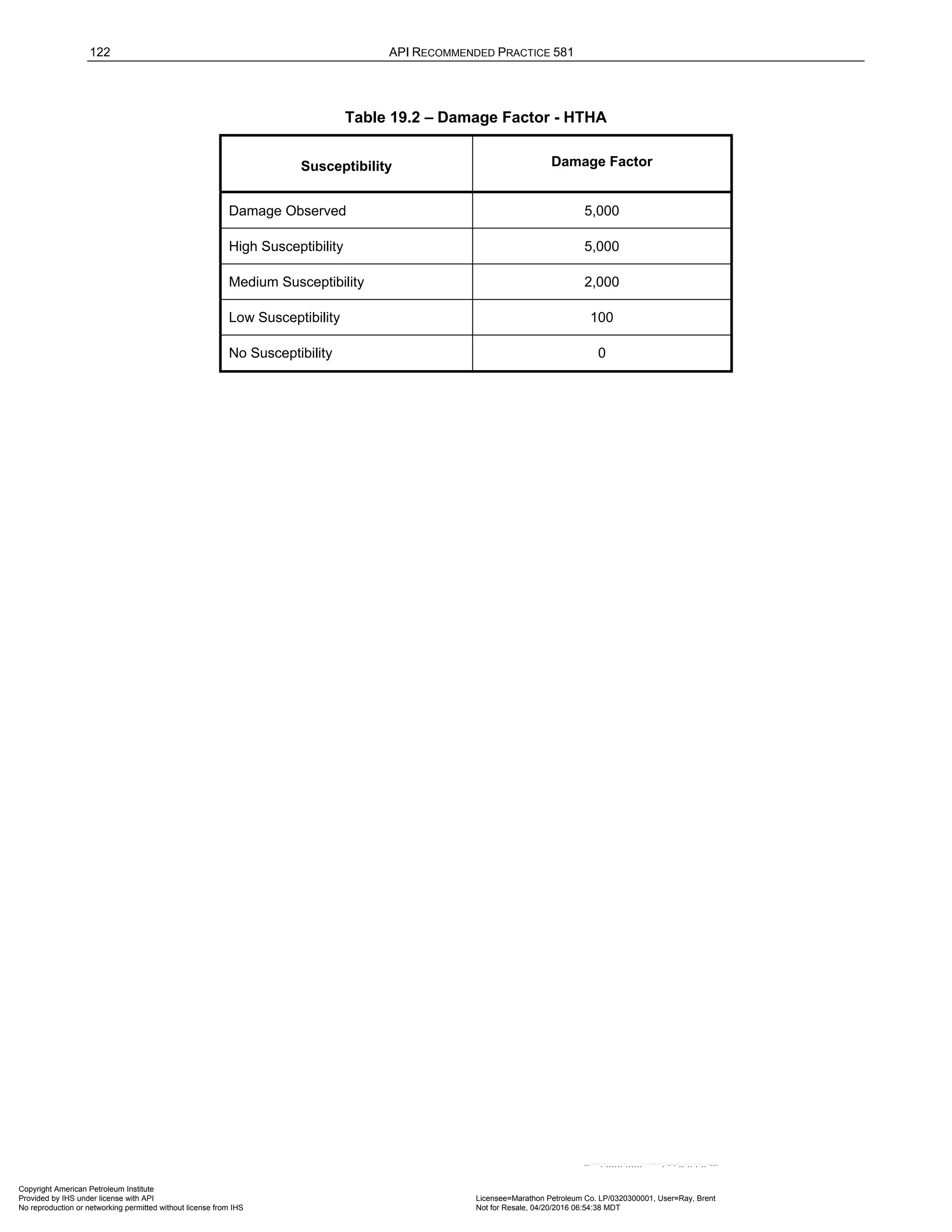
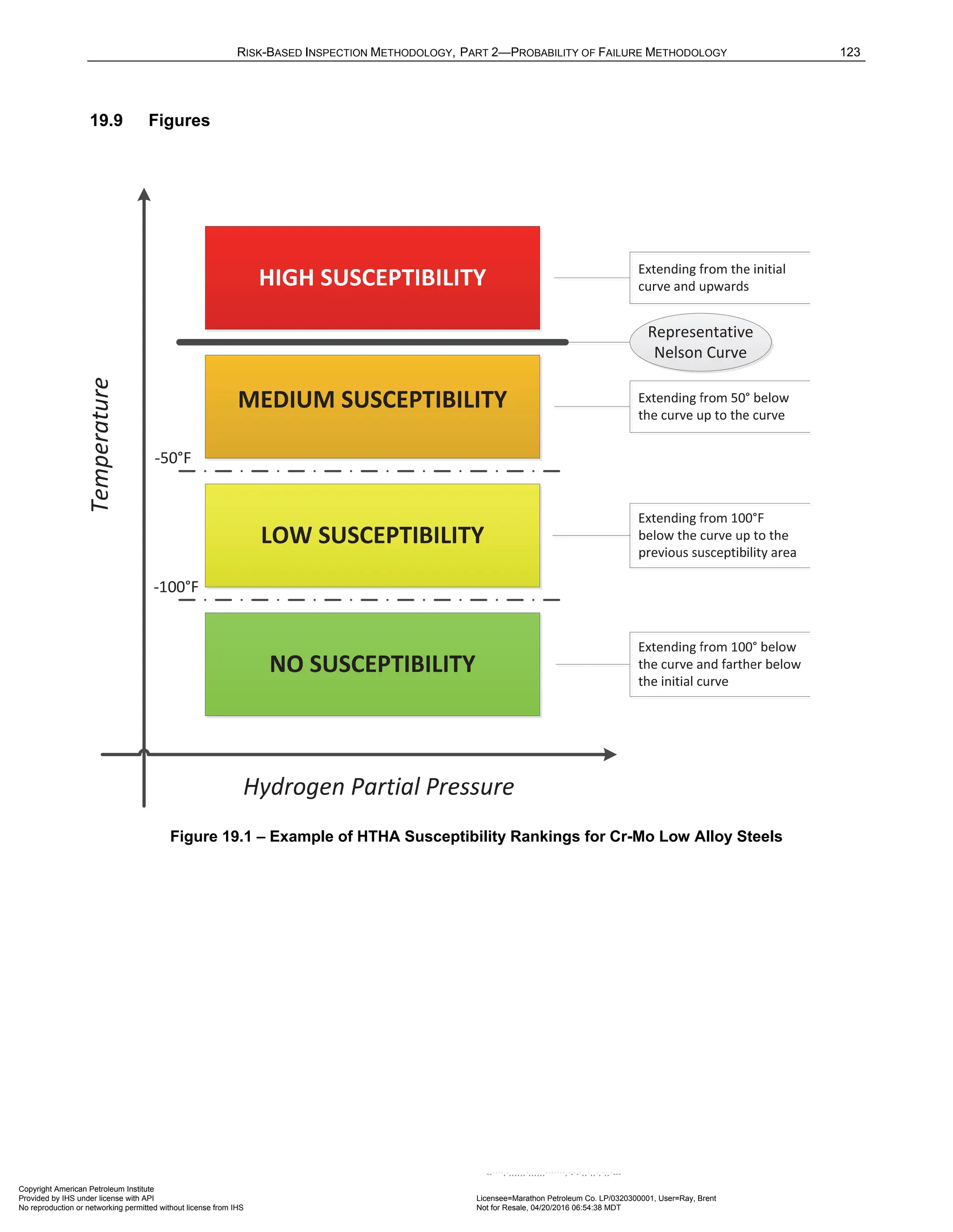
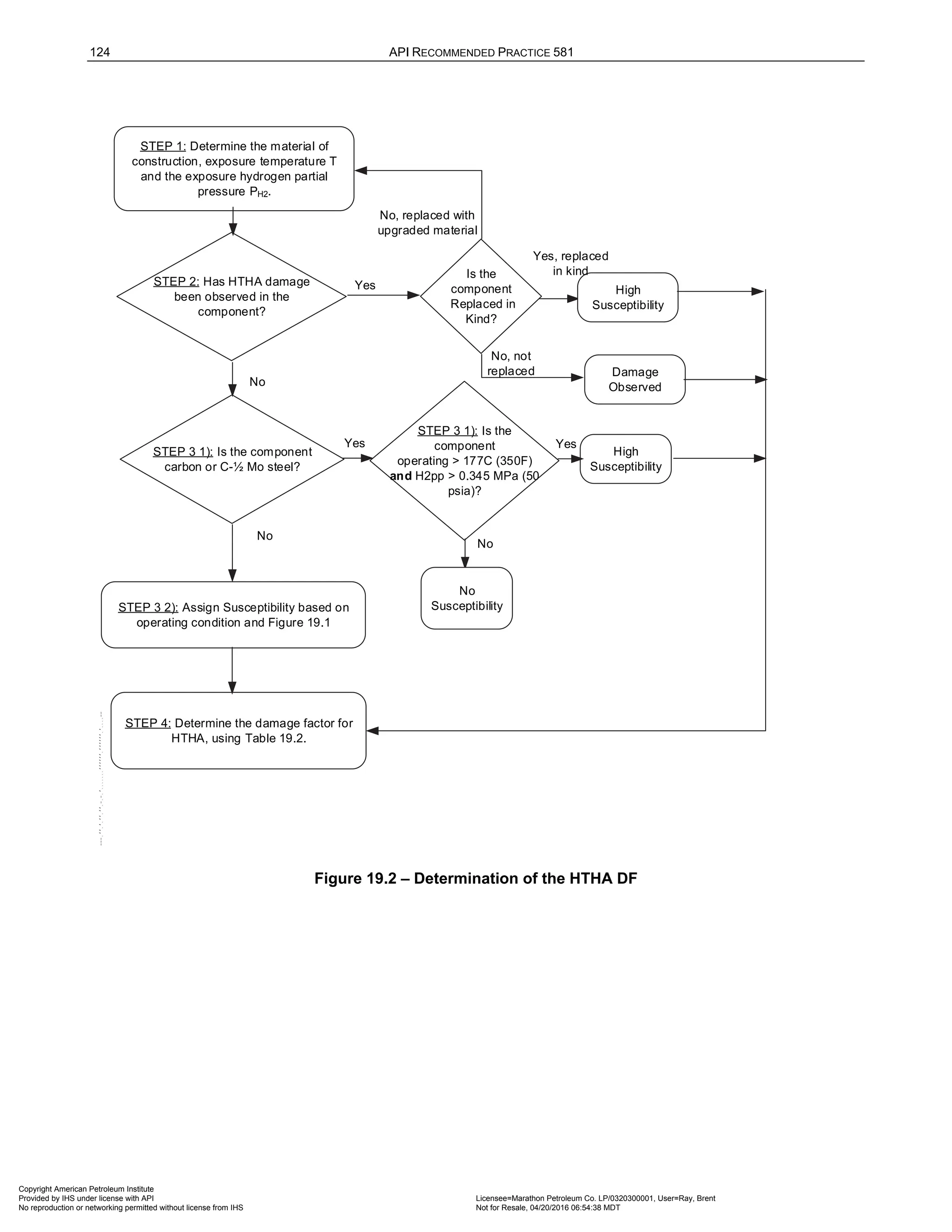
![126 API RECOMMENDED PRACTICE 581
20.6 Determination of the Damage Factor
20.6.1 Overview
A flow chart of the steps required to determine the DF for brittle fracture is shown in Figure 20.1. The following
sections provide additional information and the calculation procedure.
20.6.2 Inspection Effectiveness
Low temperature/low toughness fracture is prevented by a combination of appropriate design and operating
procedures. When low temperature/low toughness fracture does occur, it almost invariably initiates at some pre-
existing crack-like defect. From the initiation point, a crack will grow unstable, resulting in a serious leak or
sometimes complete catastrophic rupture of the component. Theoretically, an inspection to locate and remove
such pre-existing defects would reduce the POF. However, the initiating defect can be very small, and need not
be exposed to the surface where it could be found. For this reason, inspection for such defects is generally not
considered to be an effective method for prevention of brittle fracture.
If existing records of a component do not indicate if it is constructed of normalized plate, then a metallurgical
examination may help resolve this. In some cases, it may be possible to remove samples of the material large
enough for testing to determine the toughness, which can also improve the accuracy of the prediction of low
temperature/low toughness fracture likelihood.
For this damage mechanism, credit is not given for inspection. However, the results of metallurgical testing
together with impact testing can be used to update the inputs to the DF calculation that may result in a change
in this value.
20.6.3 Calculation of the Damage Factor
The following procedure may be used to determine the DF for brittle fracture, see Figure 20.1.
a) STEP 1 – Determine if administrative or process controls exist that will prevent the component from being
fully pressurized below some temperature. If so, use this temperature for Critical Exposure Temperature,
C E T , and go to STEP 3.
b) STEP 2 – Determine the CET that the component may be subjected to during operation, use guidance of
Part 3, API 579-1/ASME FFS-1.
c) STEP 3 – Determine the reference temperature, ref
T , using the material Yield Strength, YS , from Table
20.3 and ASME Exemption Curve from Table 20.1, in accordance with API 579-1/ASME FFS-1 [10].
d) STEP 4 – Determine ref
CET T
− from STEP 1 or STEP 2, as applicable, ref
T is from STEP 3.
e) STEP 5 – Determine the base DF,
brit
fB
D , using the component thickness, t, and Table 20.4 or Table 20.5
based on the component PWHT condition and ref
CET T
− from STEP 4.
f) STEP 6 – Determine the DF,
brit
f
D using Equation (2.86).
brit brit
f fb SE
D D F
= ⋅ (2.86)
In general, the adjustment factor for service experience is 1 or 1.00
SE
F = . However, this factor is reduced to
FSE = 0.01, if the component under assessment has a thickness less than or equal to 12.7 mm (0.5 inch) or
meets all of the following criteria:
1) It is fabricated from P-1 and P-3 steels where the design temperature is less than or equal to 343°C (650°F).
2) The equipment satisfied all requirements of a recognized code or standard at the time of fabrication.
3) The nominal operating conditions have been essentially the same and consistent with the specified design
conditions for a significant period of time, and more severe conditions (i.e., lower temperature and/or higher
stress) are not expected in the future.
Copyright American Petroleum Institute
Provided by IHS under license with API Licensee=Marathon Petroleum Co. LP/0320300001, User=Ray, Brent
Not for Resale, 04/20/2016 06:54:38 MDT
No reproduction or networking permitted without license from IHS
--````,`,,,,,,`,,,,,,```````,`-`-`,,`,,`,`,,`---](https://image.slidesharecdn.com/api581-3rdedition-april2016-240227010601-3bf73ab5/75/Norma-API-581-3rd-Edition-April-2016-pdf-259-2048.jpg)
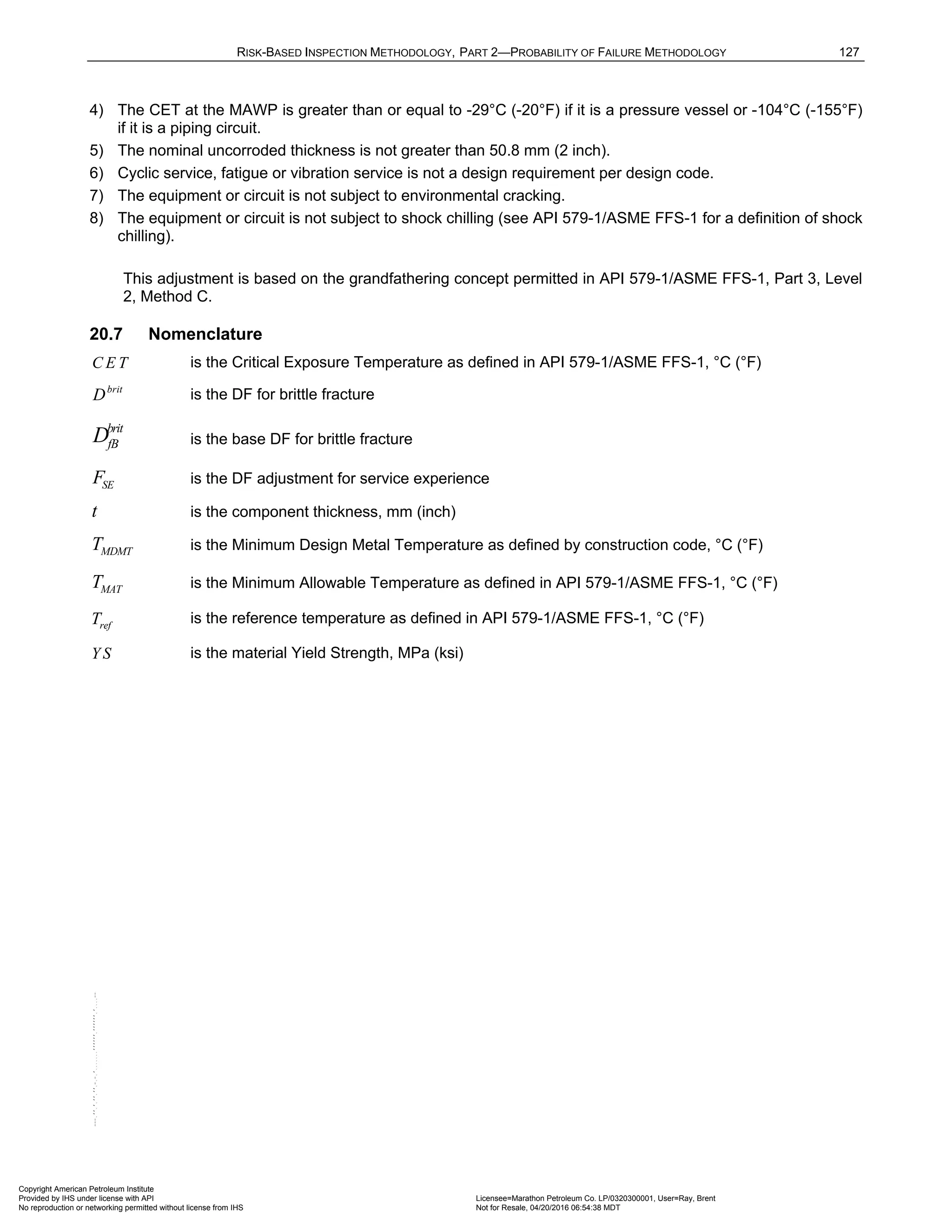
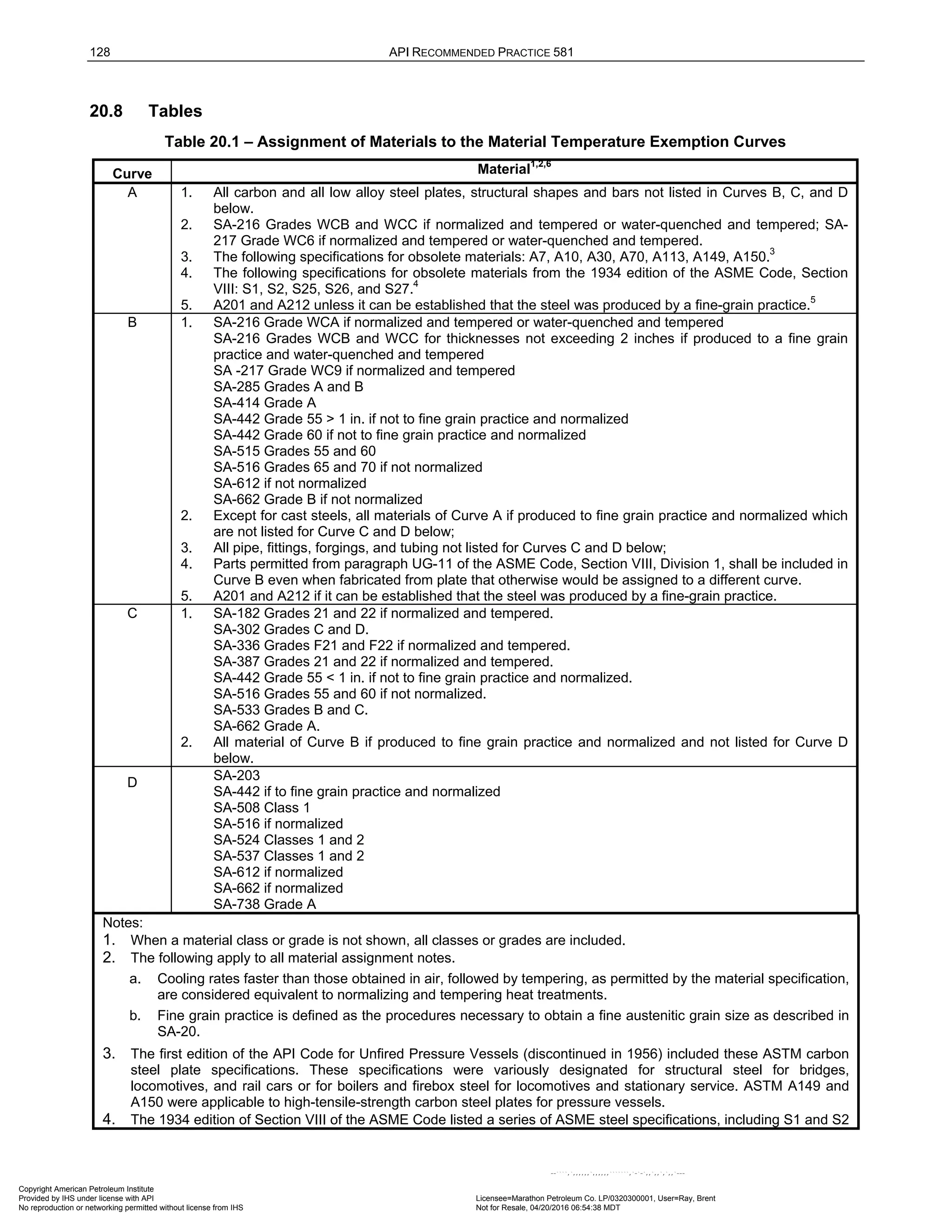
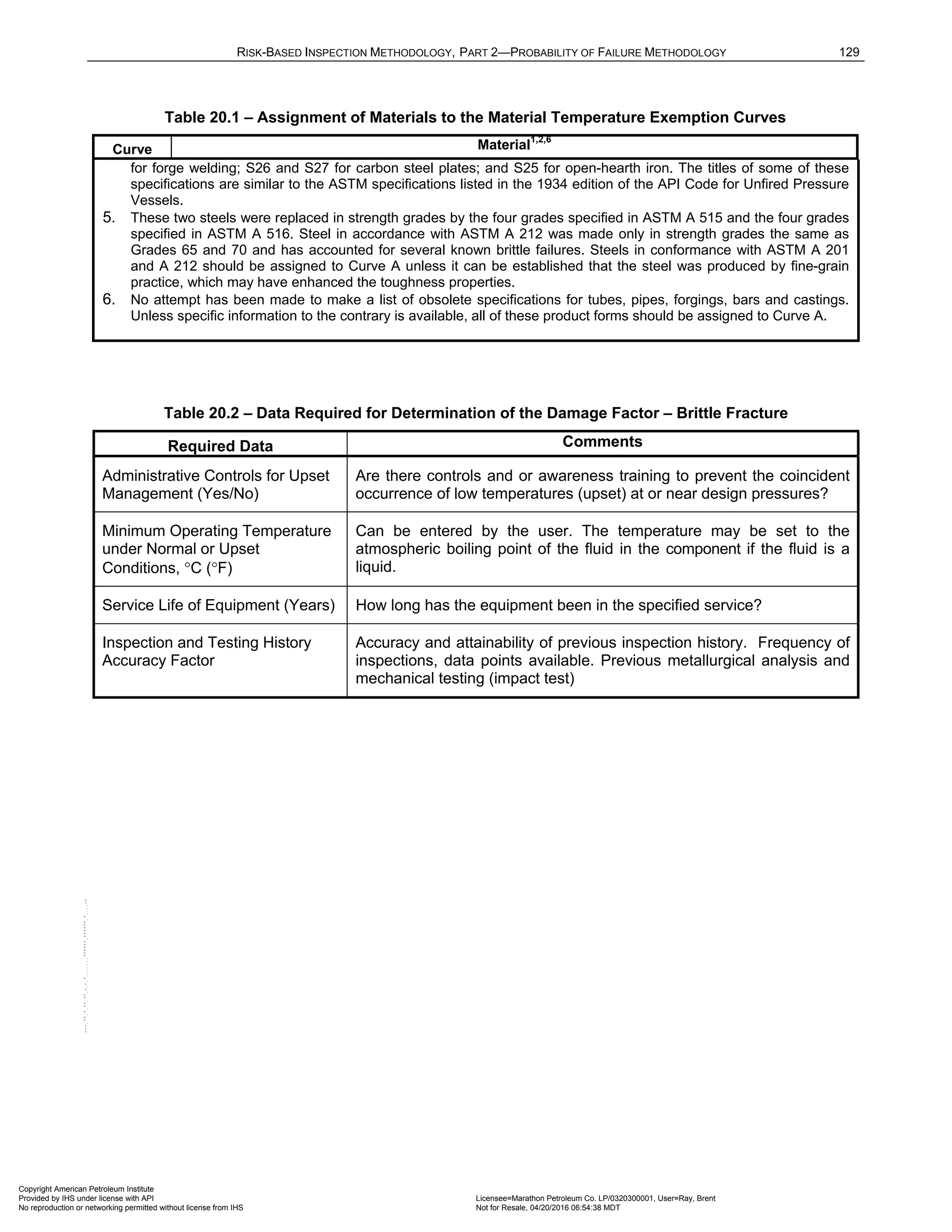
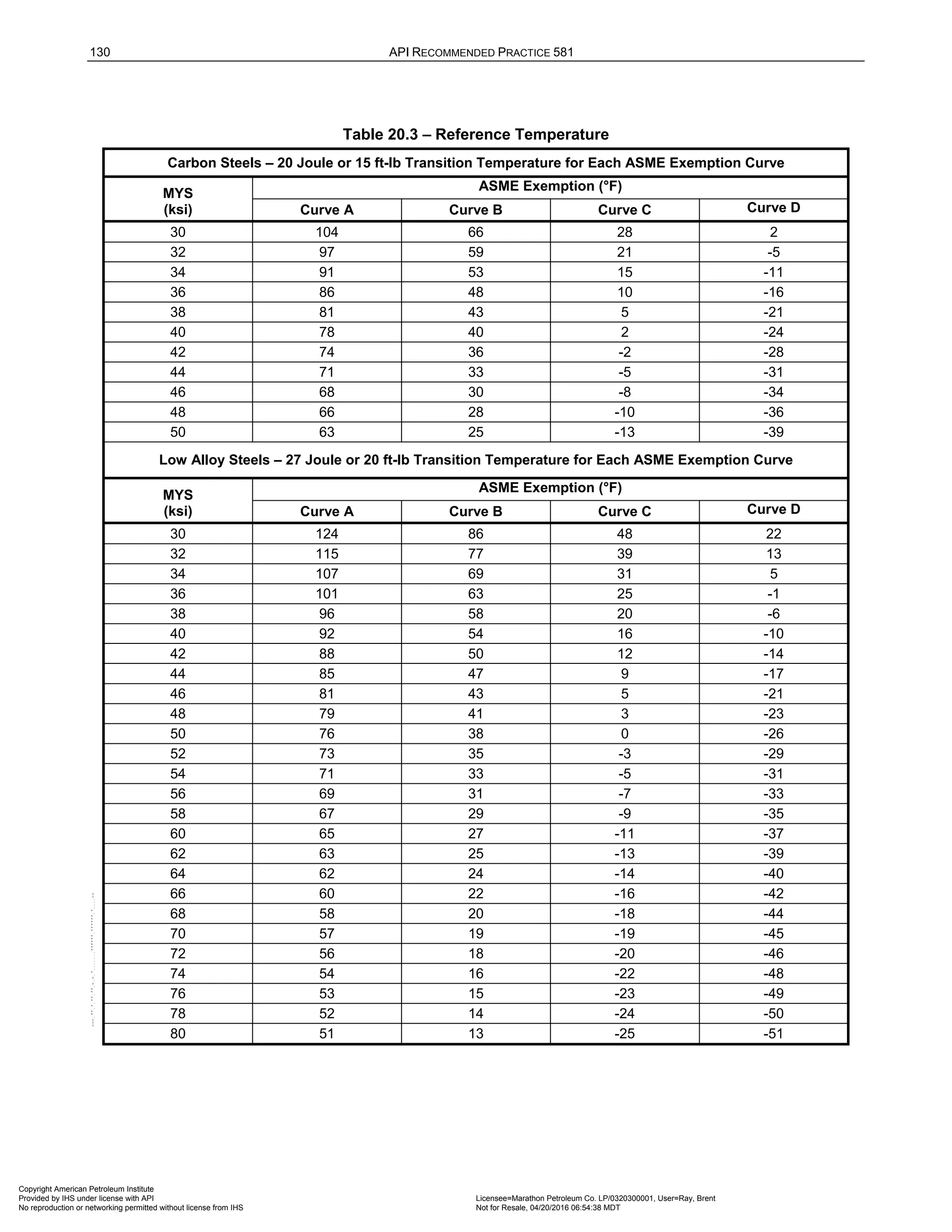
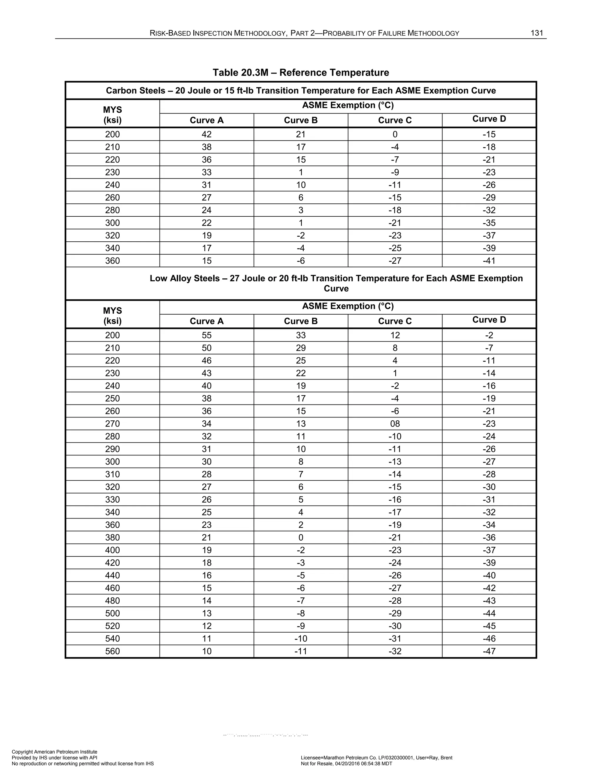
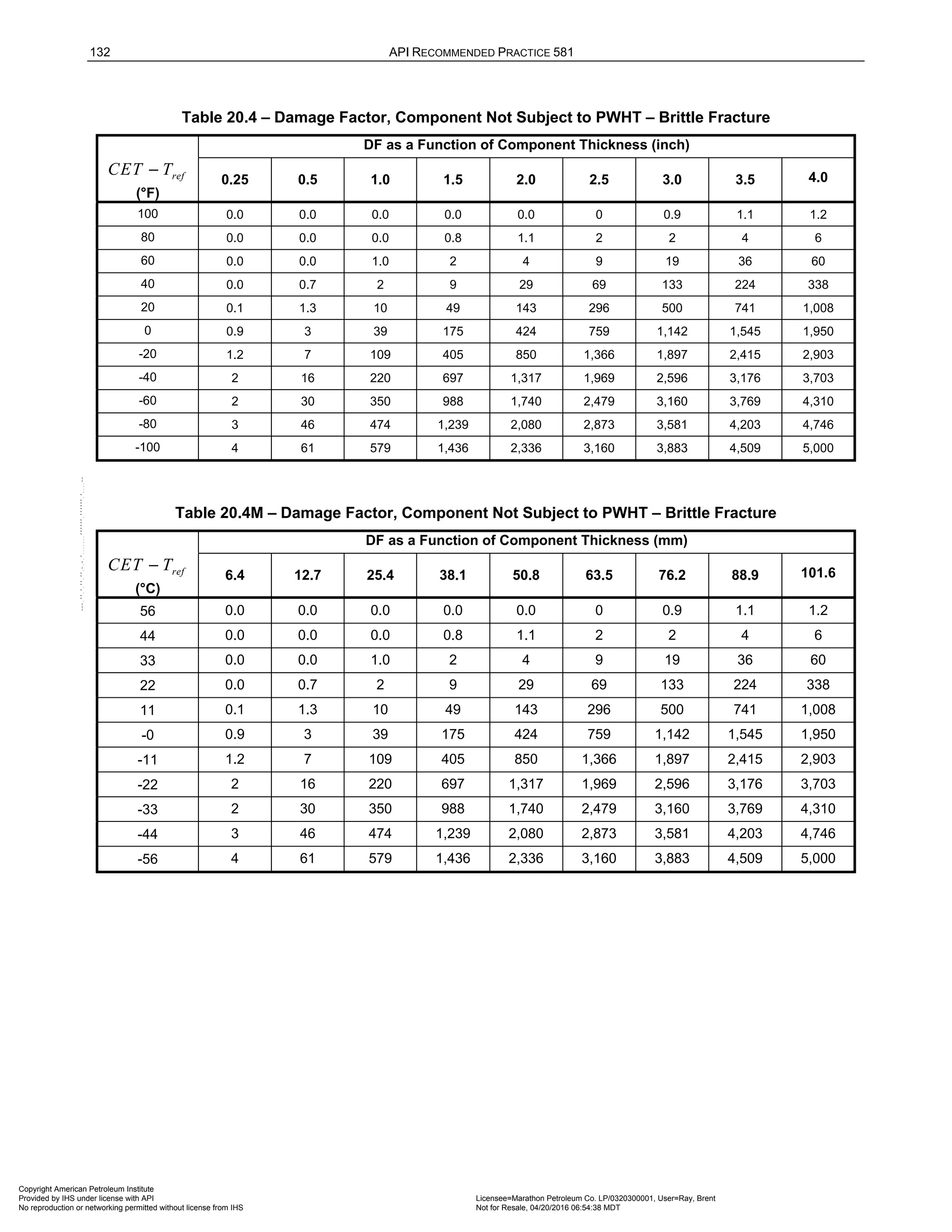
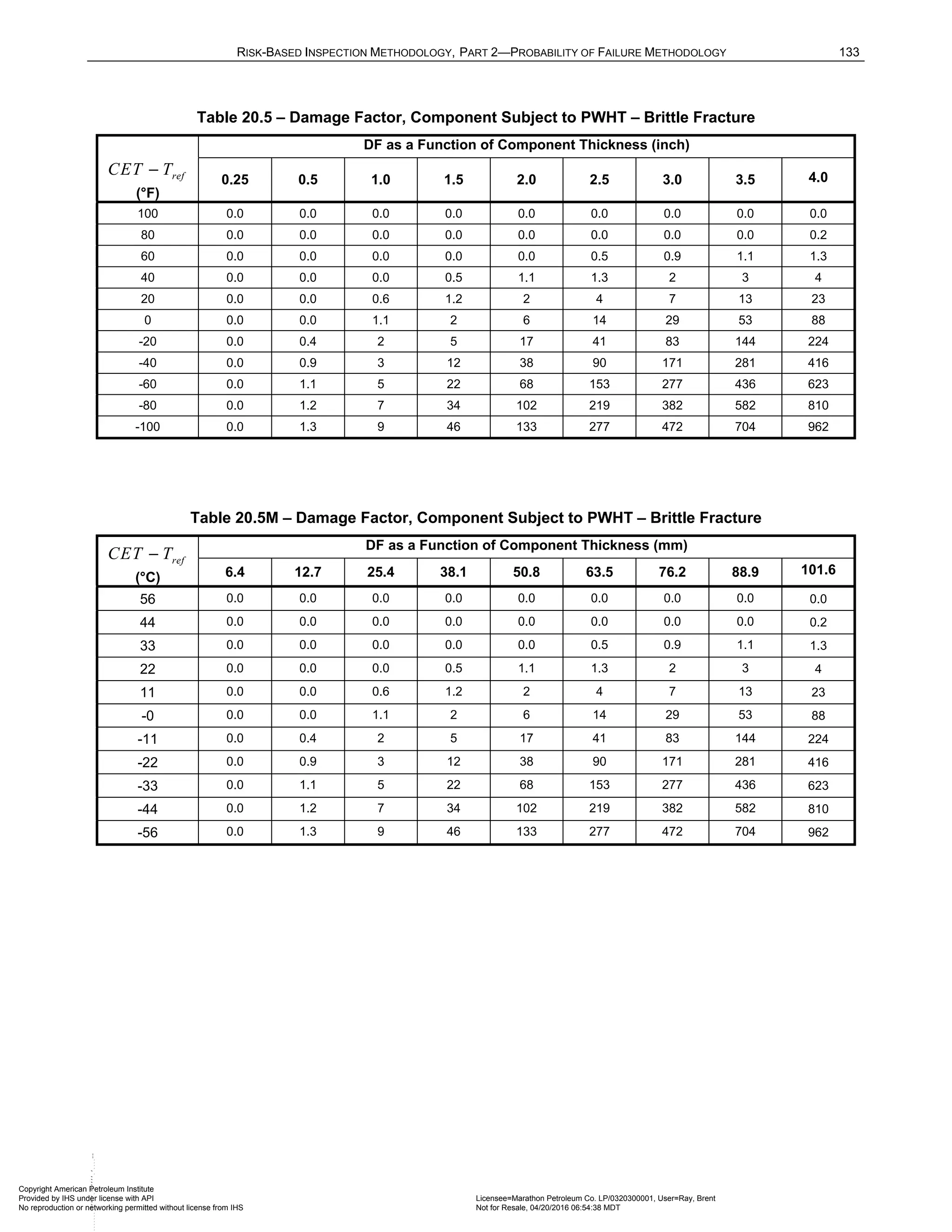
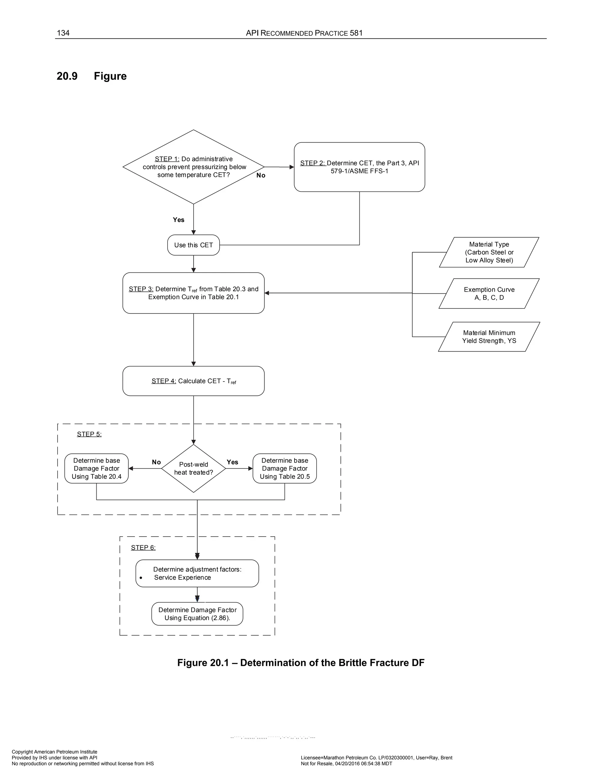
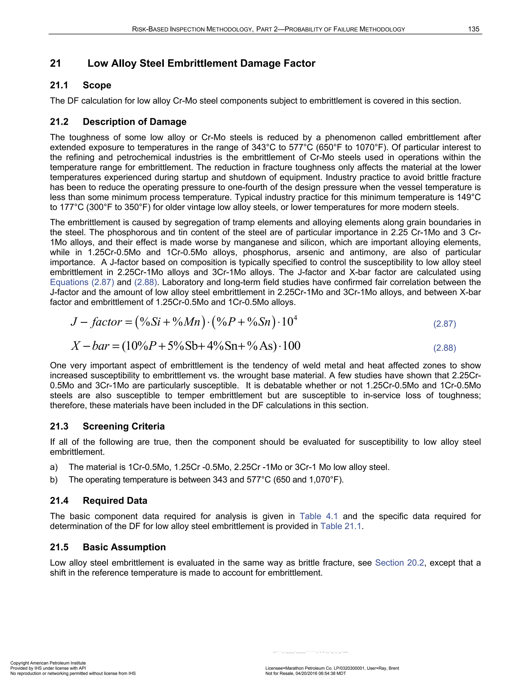
![136 API RECOMMENDED PRACTICE 581
21.6 Determination of the Damage Factor
21.6.1 Overview
A flow chart of the steps required to determine the DF for low alloy steel embrittlement is shown in Figure 21.1.
The following sections provide additional information and the calculation procedure.
21.6.2 Inspection Effectiveness
For this damage mechanism, credit is not given for inspection. However, the results of metallurgical testing
together with impact testing can be used to update the inputs to the DF calculation that may result in a change
in this value.
21.6.3 Calculation of the Damage Factor
The following procedure may be used to determine the DF for low alloy steel embrittlement, see Figure 21.1.
a) STEP 1 – Determine if administrative or process controls exist that will prevent the component from being
fully pressurized below some temperature. If so, use this as the Minimum Pressurization Temperature,
MPT
T , and go to STEP 3.
b) STEP 2 – Determine the MPT
T that the component may be subjected to during operation, use the lowest of
the following:
1) The minimum design temperature, MDT
T
2) The MPT
T as estimated by the process engineer, including upsets
c) STEP 3 – Determine the reference temperature, ref
T , from Table 20.3 using material Yield Strength, Y S ,
and the ASME Exemption Curve from Table 20.1 [10].
d) STEP 4 – Determine FATT
Δ . If FATT
Δ is not known it may be estimated by one of the following
methods, listed in decreasing order of accuracy.
1) Determined by engineering analysis or actual impact testing of metal samples.
2) Determined in a step cooling embrittlement test, S C E . The S C E can be related to the actual in-service
FATT
Δ using Equation (2.89) where age is the operating time in hours and SCE is the specified change
in FATT .
[ ]
( )
0.67 log 0.91
FATT age SCE
Δ = ⋅ − ⋅
(2.89)
3) Determined by chemical composition correlations. Use the chemical composition to determine the J-factor
or X-bar factor using Equations (2.87) and (2.88). The J-factor and X-bar factor may be correlated to the
expected FATT
Δ after long-term service. Based on long term exposures, this is conservatively correlated
to the J-factor and x-bar factor in Equations (2.90) and (2.91), respectively.
4 2
77.321 (0.57570 ) (5.5147 (10 ) ( ))
FATT J factor J factor
Δ = − + ⋅ − − ⋅ ⋅ − (2.90)
2
87.335 (11.437 ) (0.1472 ( bar ))
FATT X bar X
Δ = − + ⋅ − − ⋅ − (2.91)
4) Determined by using conservative assumptions based on year of fabrication. A conservative value of can
be assumed for the long term FATT
Δ depending on the year of fabrication as follows:
a) 4th
generation equipment (after to 1988): 66°C (150°F)
b) 3rd
generation equipment (1981 to 1987): 121°C (250°F)
c) 2nd
generation equipment (1973 to 1980): 149°C (300°F)
d) 1st
generation equipment (1965 to 1972): 177°C (350°F)
e) STEP 5 – Calculate ref
T FATT
+ Δ using ref
T from STEP 3 and FATT
Δ from STEP 4.
Copyright American Petroleum Institute
Provided by IHS under license with API Licensee=Marathon Petroleum Co. LP/0320300001, User=Ray, Brent
Not for Resale, 04/20/2016 06:54:38 MDT
No reproduction or networking permitted without license from IHS
--````,`,,,,,,`,,,,,,```````,`-`-`,,`,,`,`,,`---](https://image.slidesharecdn.com/api581-3rdedition-april2016-240227010601-3bf73ab5/75/Norma-API-581-3rd-Edition-April-2016-pdf-269-2048.jpg)
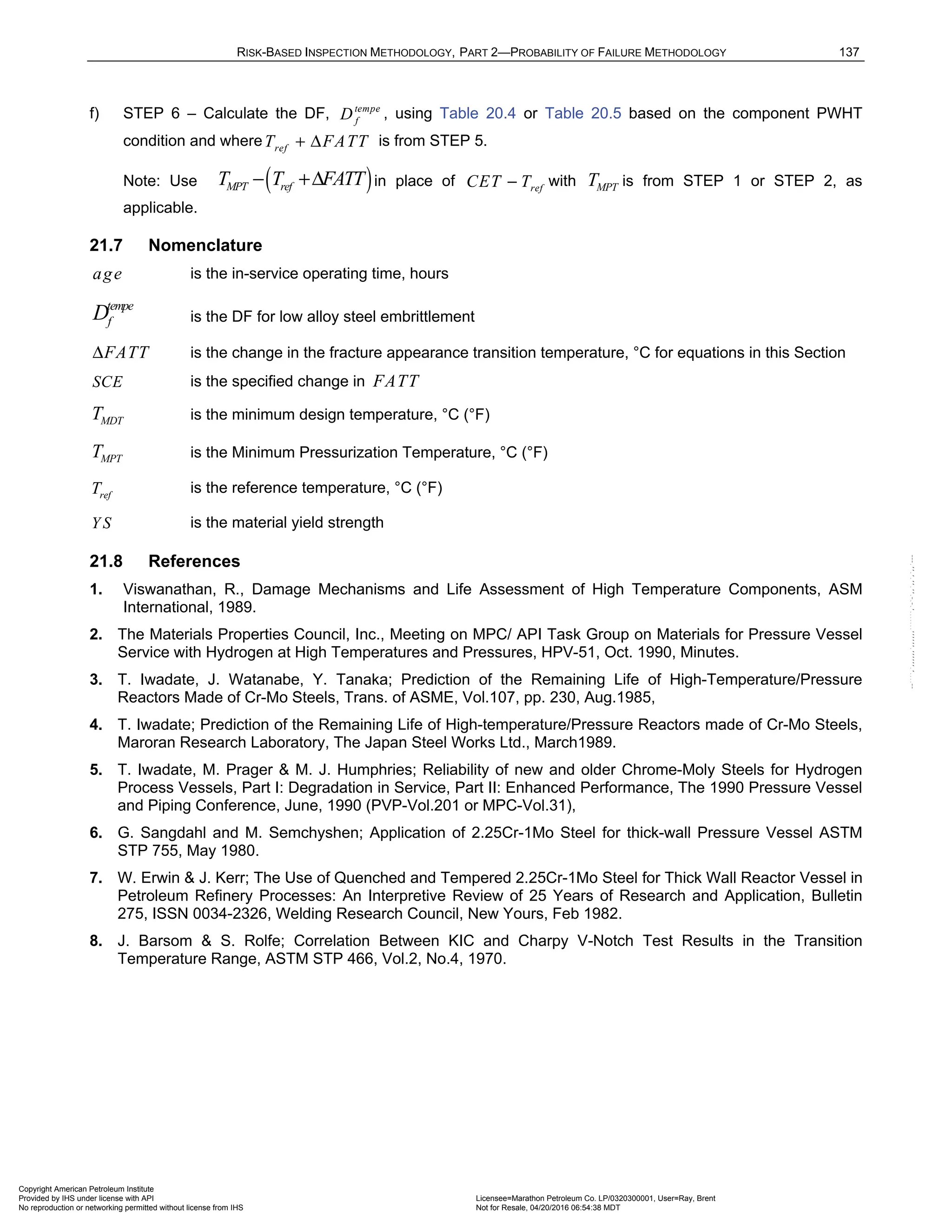
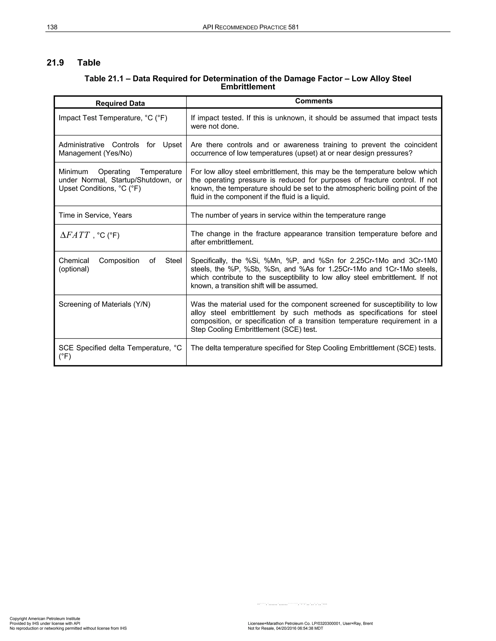
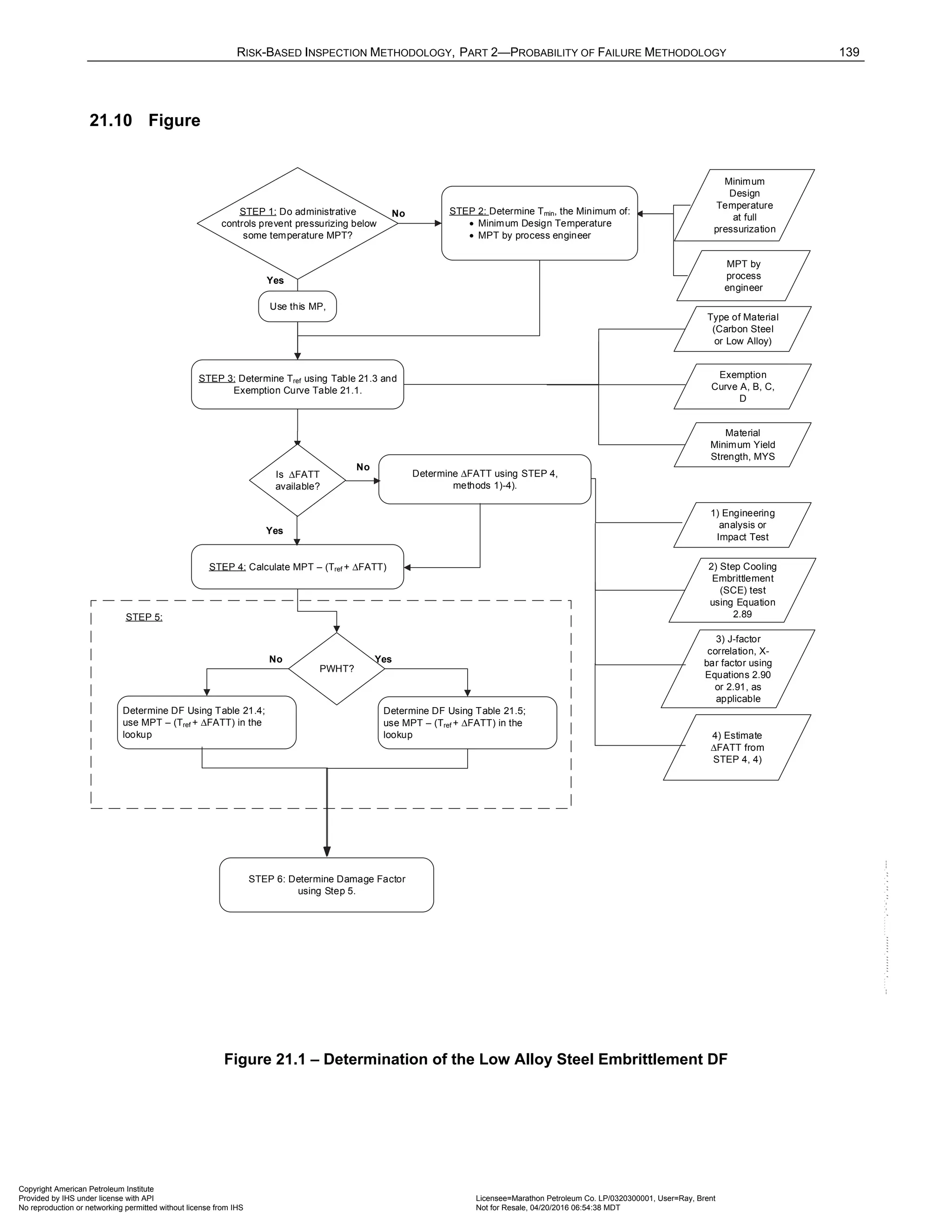
![140 API RECOMMENDED PRACTICE 581
22 885°F Embrittlement Damage Factor
22.1 Scope
The DF calculation for components subject to 885°F embrittlement is covered in this section.
22.2 Description of Damage
885°F embrittlement is a reduction in toughness of ferritic stainless steels with a chromium content of greater
than 13%, after exposure to temperatures between 371°C and 538°C (700°F and 1000°F). The reduction in
toughness is due to precipitation of a chromium-phosphorous intermetallic phase at elevated temperatures. As
is the case with other mechanisms that result in a loss of toughness due to metallurgical changes, the effect on
toughness is most pronounced not at the operating temperature, but at lower temperatures experienced during
plant shutdowns or upsets.
The precipitation of the intermetallic phase is believed to occur most readily at a temperature around 474°C
(885°F), hence the name for this mechanism. Steels with more than 27% chromium are most severely affected,
but these are not typically used in refinery or petrochemical processes. Martensitic stainless steels such as Type
410 are normally considered to be immune to this problem. Type 405 is a ferritic stainless steel that is subject to
the problem if it contains chromium levels at the high end of its composition range.
The existence of 885o
F embrittlement can reveal itself by an increase in hardness in affected areas. Physical
testing of samples removed from service is the most positive indicator of a problem.
885o
F embrittlement is reversible by appropriate heat treatment to dissolve precipitates, followed by rapid
cooling. Heat treatment temperature is typically in the range of 760°C to 816°C (1,400°F to 1,500°F), so this
may not be practical for many components.
22.3 Screening Criteria
If both of the following are true, then the component should be evaluated for susceptibility to 885o
F
embrittlement:
a) The material is a high chromium (>12% Cr) ferritic steel
b) The operating temperature is between 371°C and 566°C (700°F and 1,050 °F)
22.4 Required Data
The basic component data required for analysis is given in Table 4.1 and the specific data required for
determination of the DF for 885°F embrittlement is provided in Table 22.1.
22.5 Basic Assumption
Since 885°F embrittlement may occur in a relatively short period of time, it is assumed in the development of the
DF that any of the ferritic materials listed in Table 22.2 that have been exposed to temperatures in the 371°C to
538°C (700°F to 1,000°F) range are affected.
API 579-1/ASME FFS-1 [3] recommends that for embrittled materials, the toughness should be determined by
the Ir
K (fracture arrest) curves, truncated at 38°C (100°F). It is further recommended that for severely embrittled
materials, 50% of this value should be used. The ductile-to-brittle transition temperatures for ferritic stainless
steels (400 series) typically are in the 10°C to 38°C (50°F to 100°F) range.
22.6 Determination of the Damage Factor
22.6.1 Overview
A flow chart of the steps required to determine the DF for 885°F embrittlement is shown in Figure 22.1. The
following sections provide additional information and the calculation procedure.
Copyright American Petroleum Institute
Provided by IHS under license with API Licensee=Marathon Petroleum Co. LP/0320300001, User=Ray, Brent
Not for Resale, 04/20/2016 06:54:38 MDT
No reproduction or networking permitted without license from IHS
--````,`,,,,,,`,,,,,,```````,`-`-`,,`,,`,`,,`---](https://image.slidesharecdn.com/api581-3rdedition-april2016-240227010601-3bf73ab5/75/Norma-API-581-3rd-Edition-April-2016-pdf-273-2048.jpg)
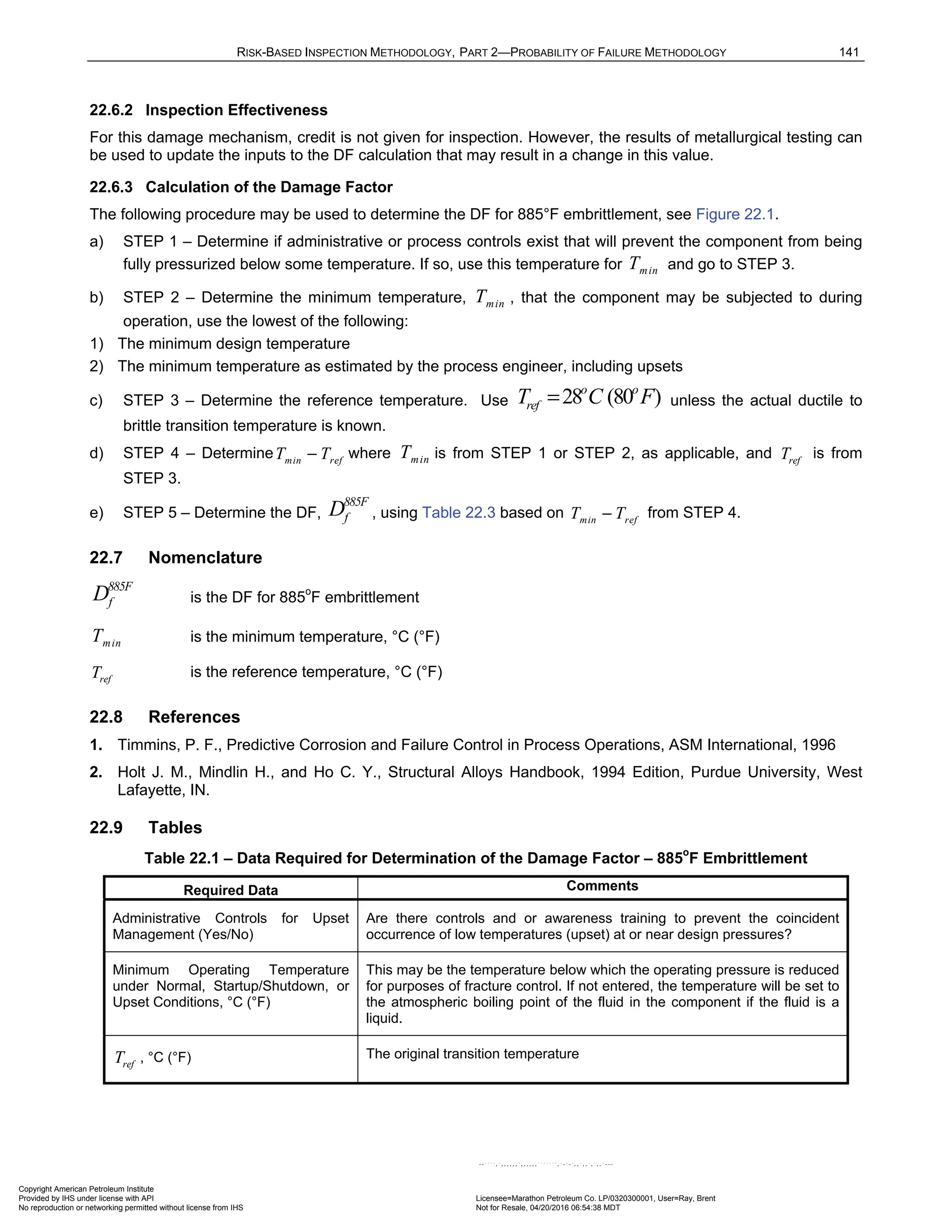
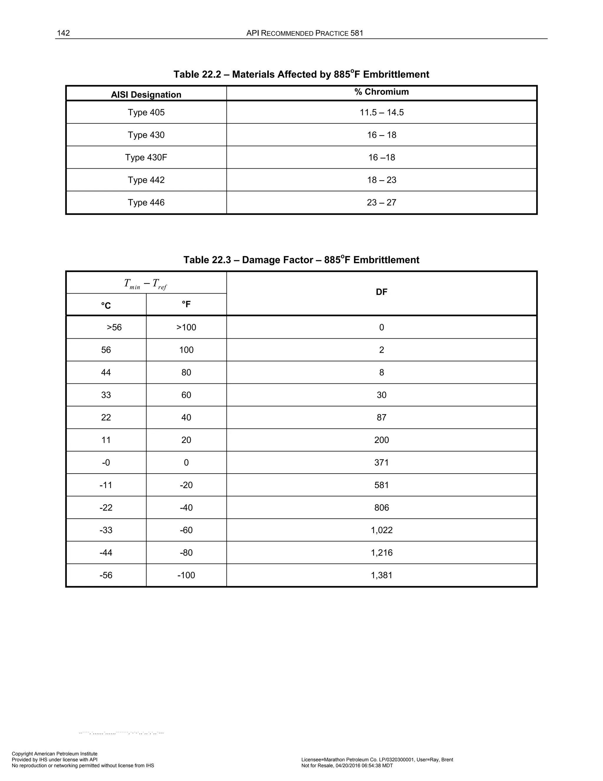
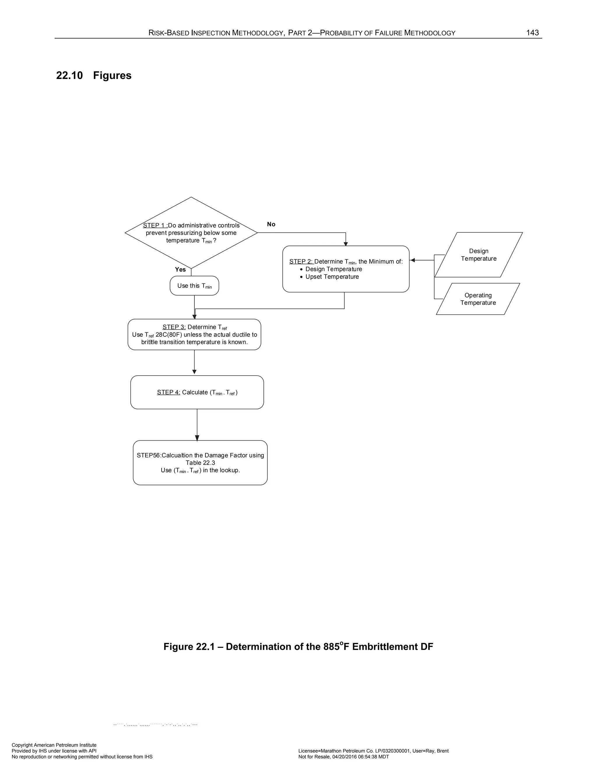
![RISK-BASED INSPECTION METHODOLOGY, PART 2—PROBABILITY OF FAILURE METHODOLOGY 145
23.3 Screening Criteria
If both of the following are true, then the component should be evaluated for susceptibility to sigma phase
embrittlement:
a) The material an austenitic stainless steel
b) The operating temperature between 593°C and 927°C (1,100 and 1,700 °F)
23.4 Required Data
The basic component data required for analysis is given in Table 4.1 and the specific data required for
determination of the DF for sigma phase embrittlement is provided in Table 23.1.
23.5 Basic Assumption
Since data is scarce and exhibits considerable scatter, it is assumed that sigmatized austenitic stainless steels
will behave in a brittle fashion similar to ferritic steels. The data available showed a reduction in properties, but
not the original properties. It is assumed that in the calculation of the DF, the original impact toughness of
austenitic stainless steels is about 330 [300 ]
MPa m ksi in
The references were searched for additional test data, which was scarce and exhibited considerable scatter.
The test data found is shown in Table 23.2. The data in this table was used to construct property trend lines of
Low Sigma (1% and 2%), High Sigma (10%), and Medium Sigma (Average of Low and High).
23.6 Determination of the Damage Factor
23.6.1 Overview
A flow chart of the steps required to determine the DF for sigma phase embrittlement is shown in Figure 23.1.
The following sections provide additional information and the calculation procedure.
23.6.2 Inspection Effectiveness
For this damage mechanism, credit is not given for inspection. However, the results of metallurgical testing can
be used to update the inputs to the DF calculation that may result in a change in this value.
23.6.3 Calculation of the Damage Factor
The following procedure may be used to determine the DF for sigma phase embrittlement, see Figure 23.1.
a) STEP 1 – Determine the evaluation temperature min
T . The material may be evaluated at normal operating
conditions, or at a lower temperature such as shutdown or upset temperature.
b) STEP 2 – Determine the estimated % sigma in the material. This can be made through comparisons with
materials in similar service, or via metallographic examination of a sample.
c) STEP 3 – Determine the DF,
sigma
f
D , using Table 23.3 based on min
T from STEP 1 and the estimated %
sigma from STEP 2.
23.7 Nomenclature
sigma
f
D is the DF for sigma phase embrittlement
min
T is the minimum temperature, °C (°F)
Copyright American Petroleum Institute
Provided by IHS under license with API Licensee=Marathon Petroleum Co. LP/0320300001, User=Ray, Brent
Not for Resale, 04/20/2016 06:54:38 MDT
No reproduction or networking permitted without license from IHS
--````,`,,,,,,`,,,,,,```````,`-`-`,,`,,`,`,,`---](https://image.slidesharecdn.com/api581-3rdedition-april2016-240227010601-3bf73ab5/75/Norma-API-581-3rd-Edition-April-2016-pdf-278-2048.jpg)

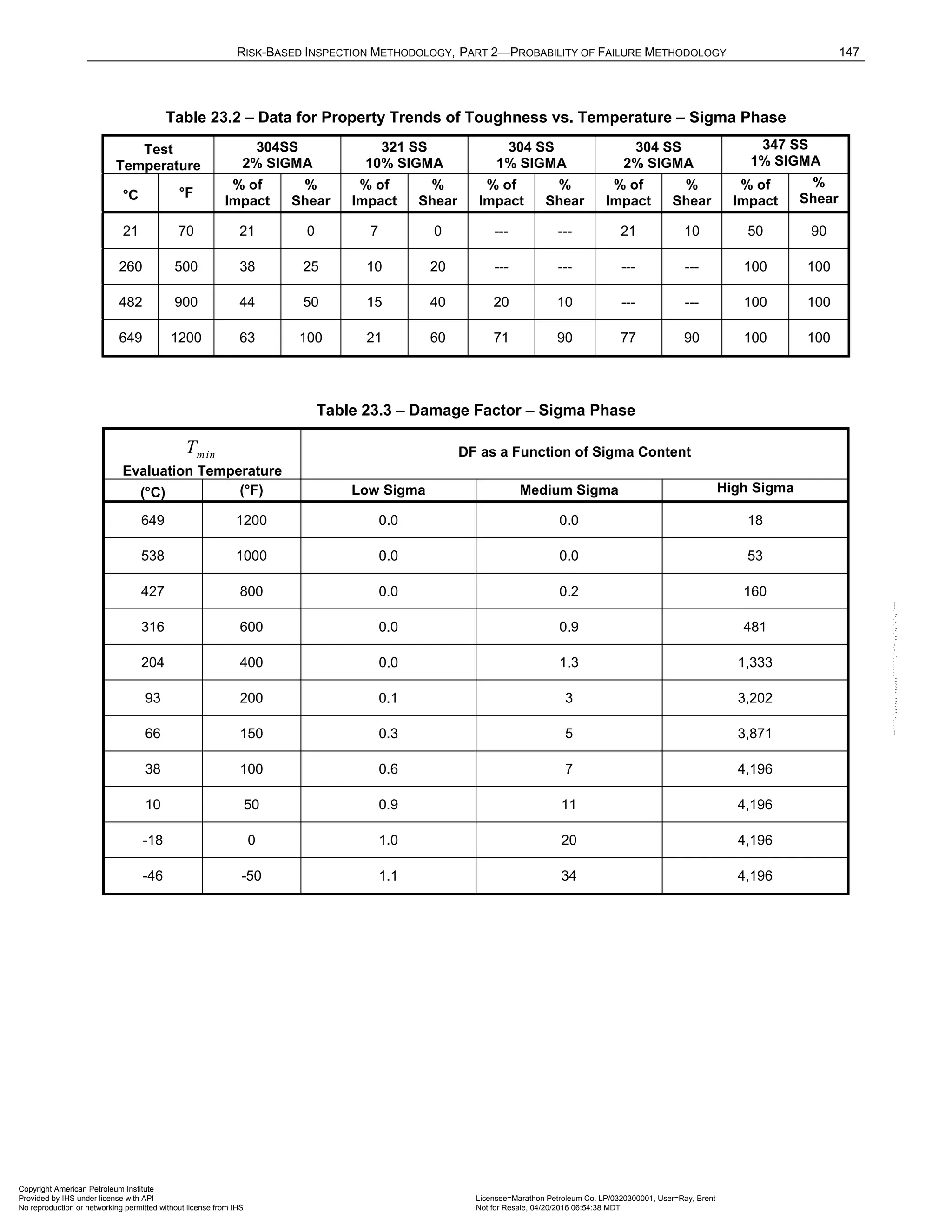
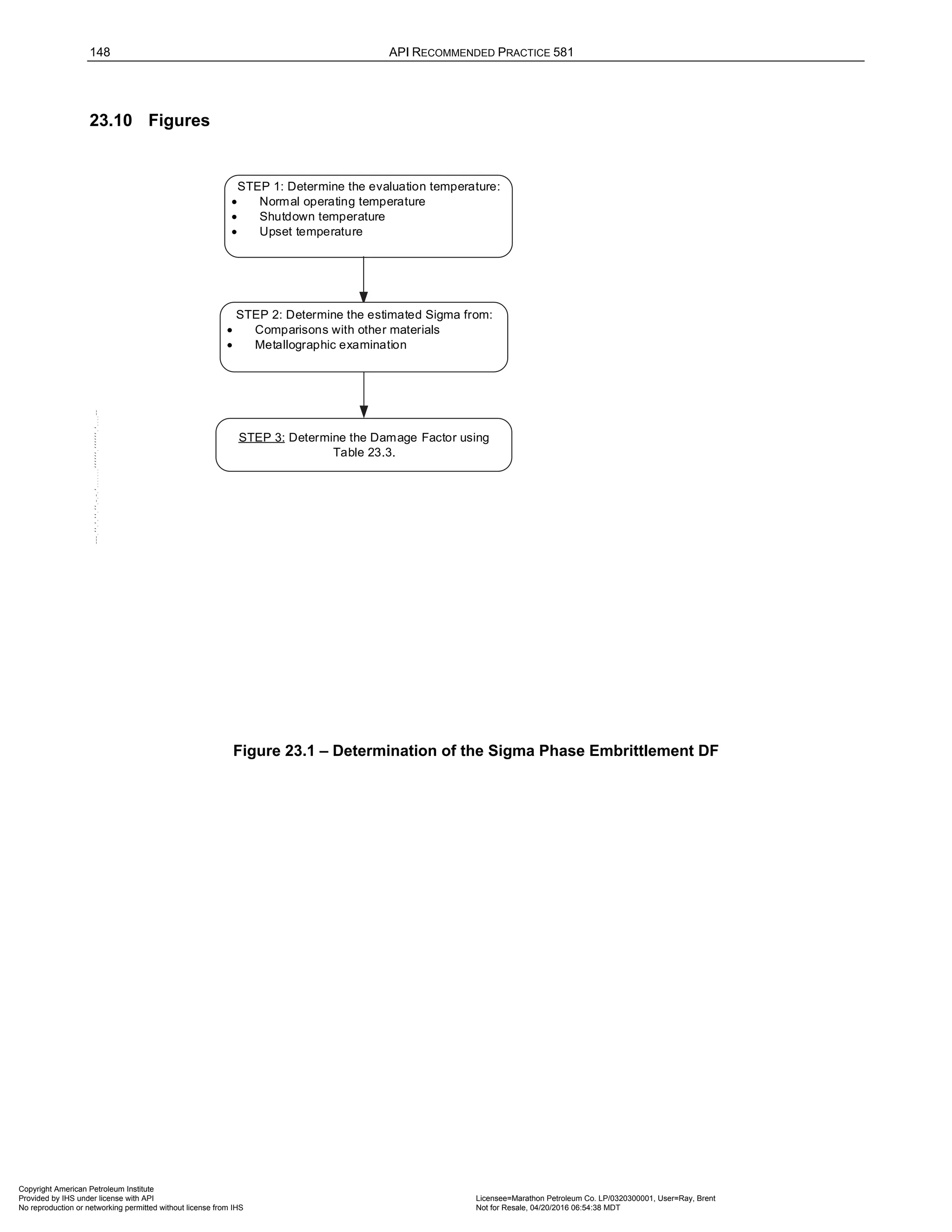
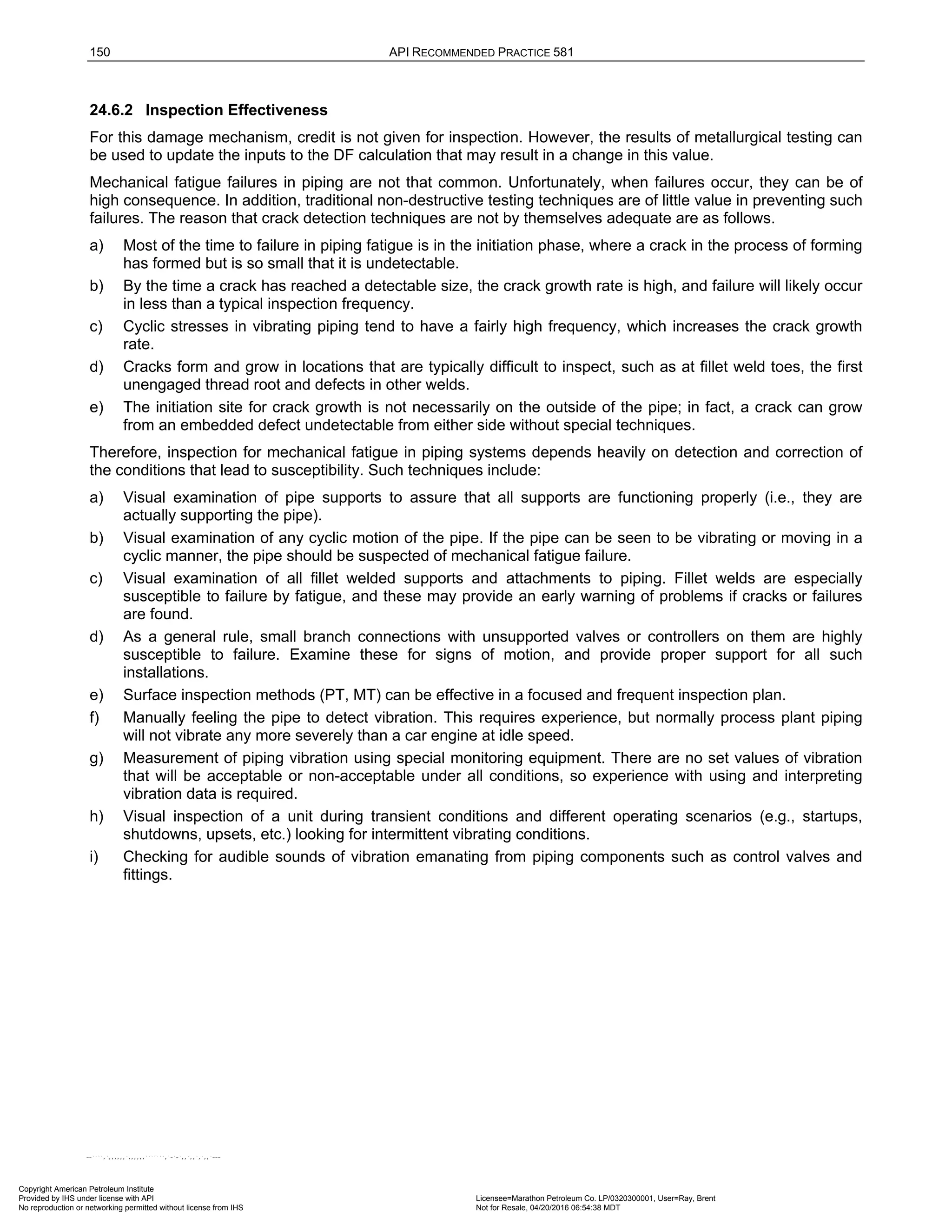


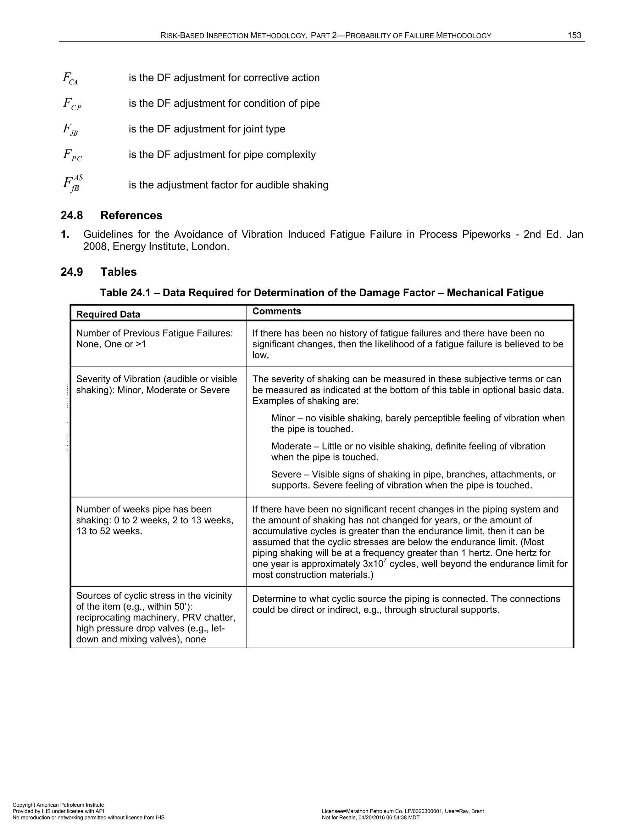
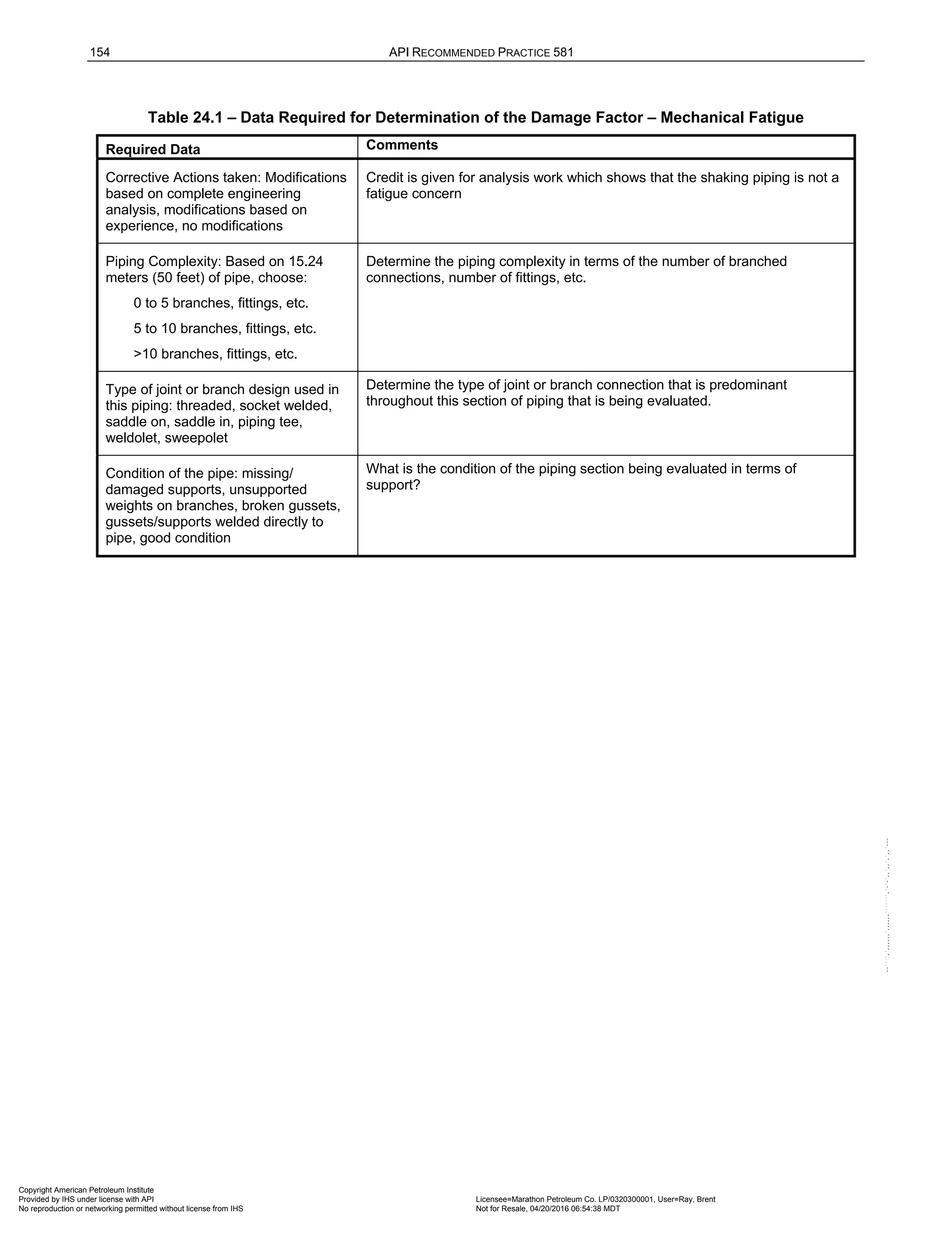
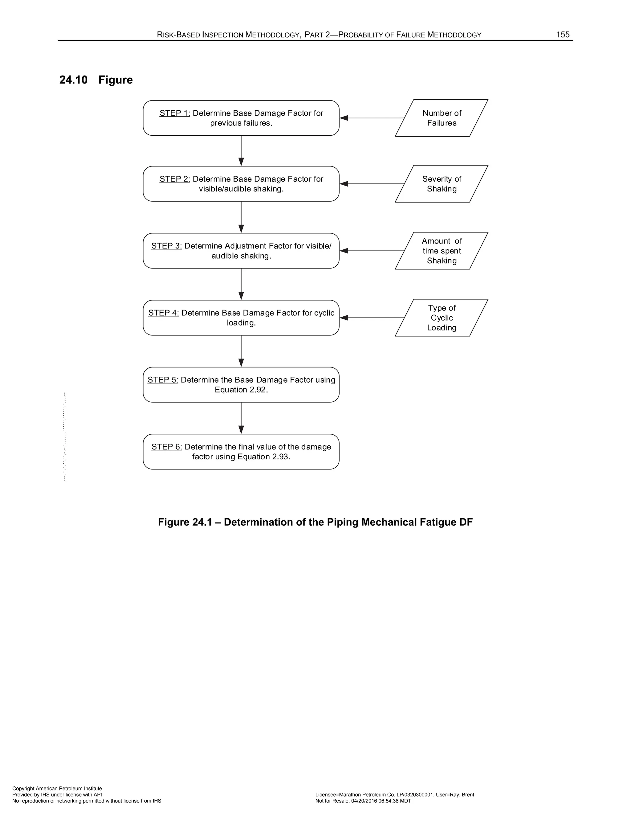

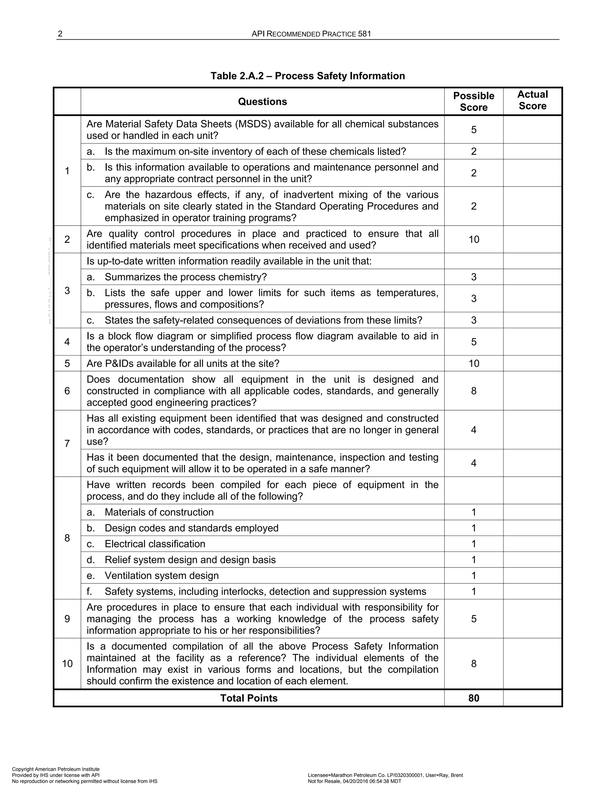
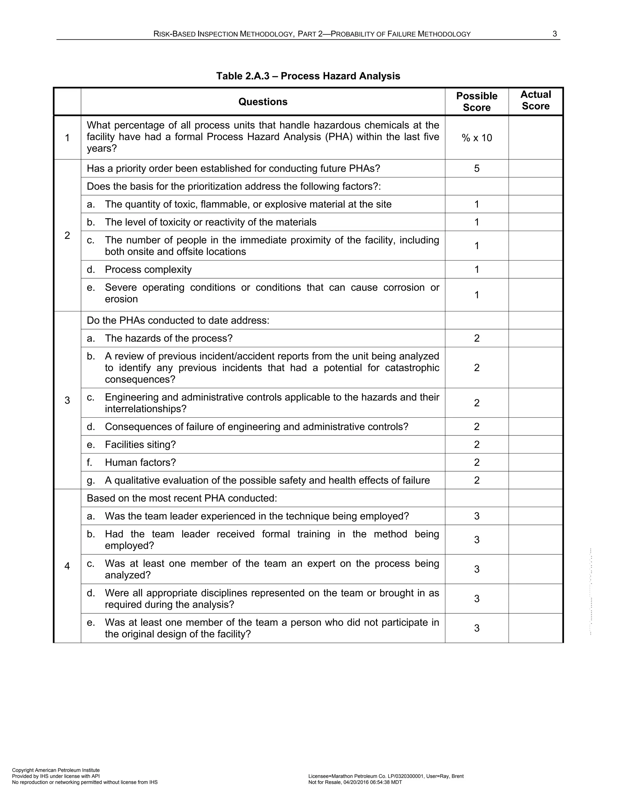
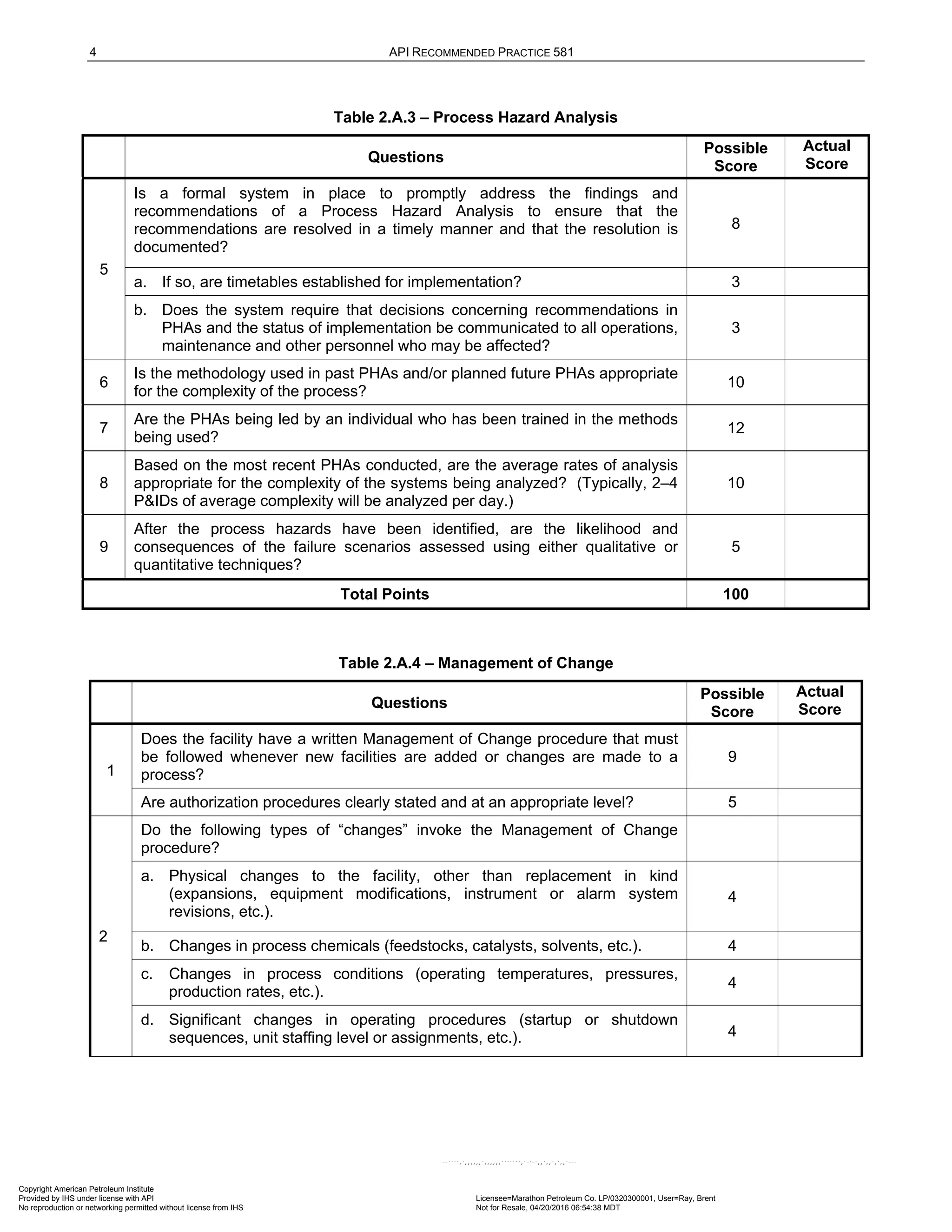

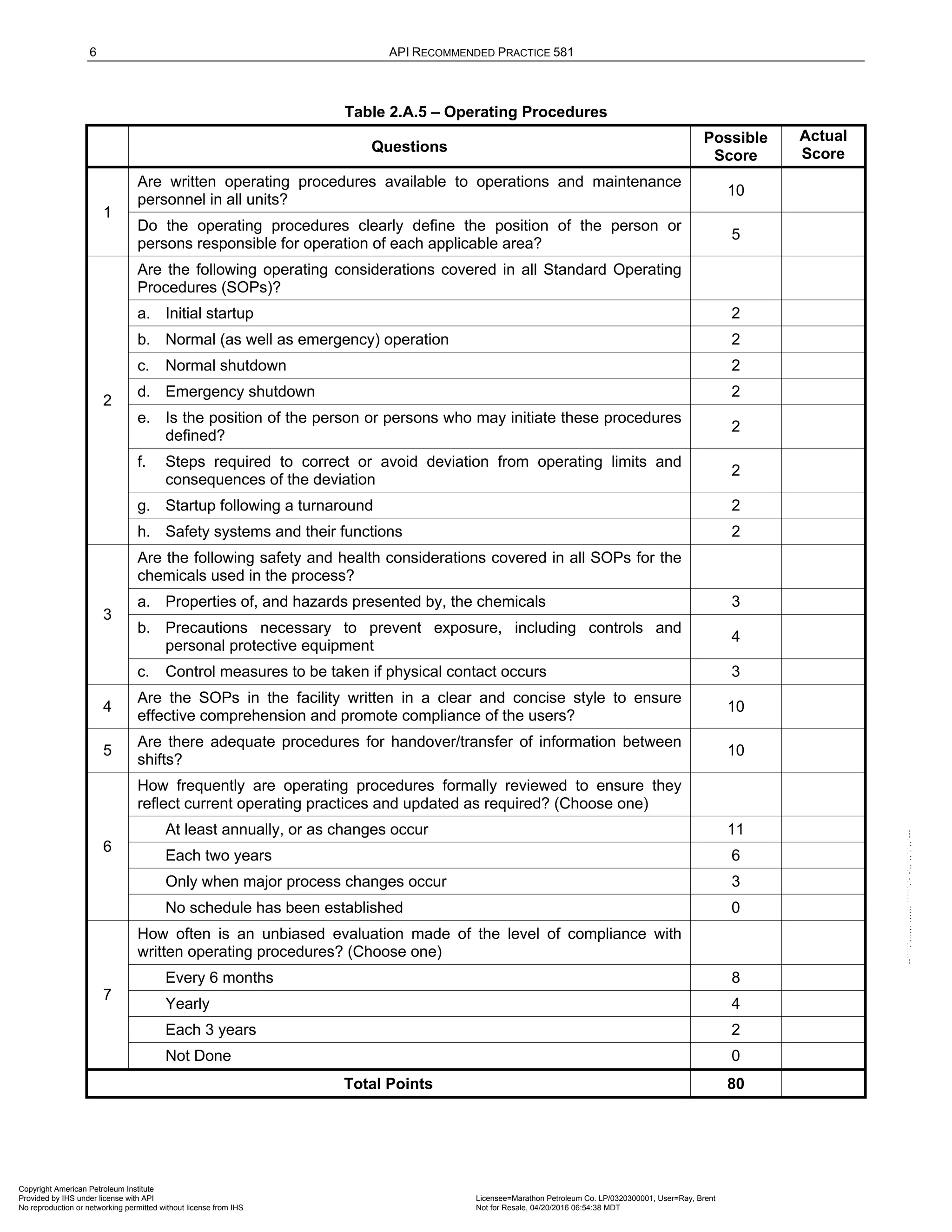
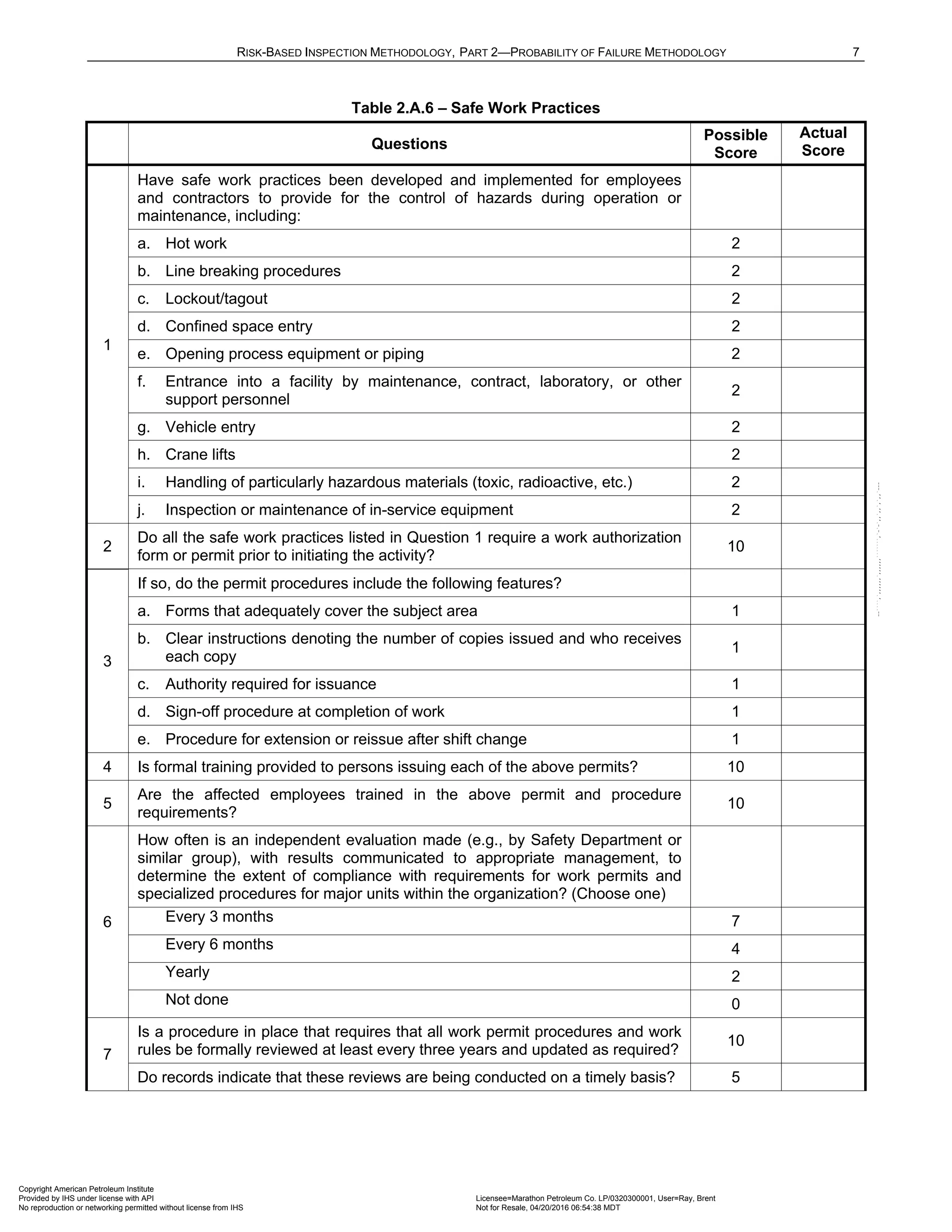
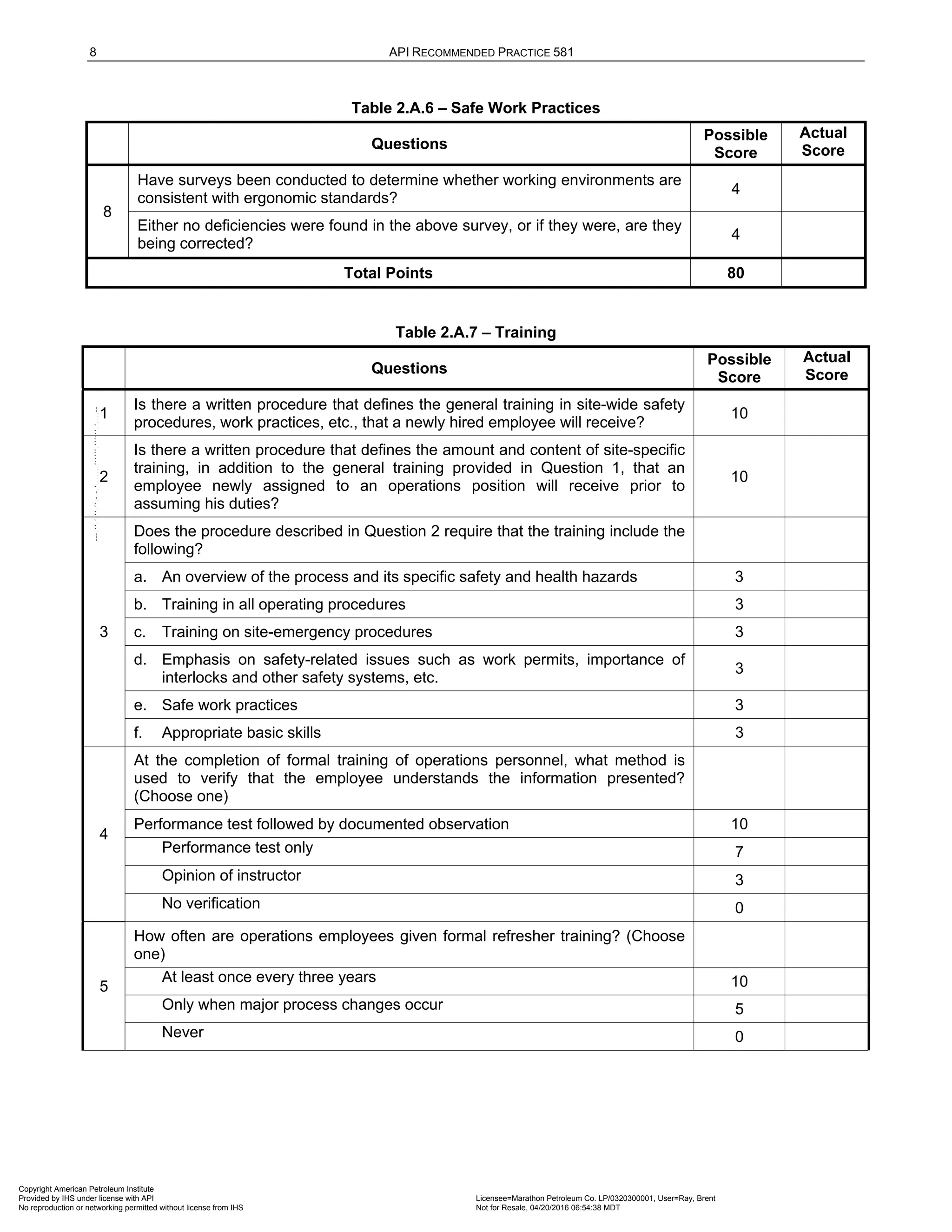
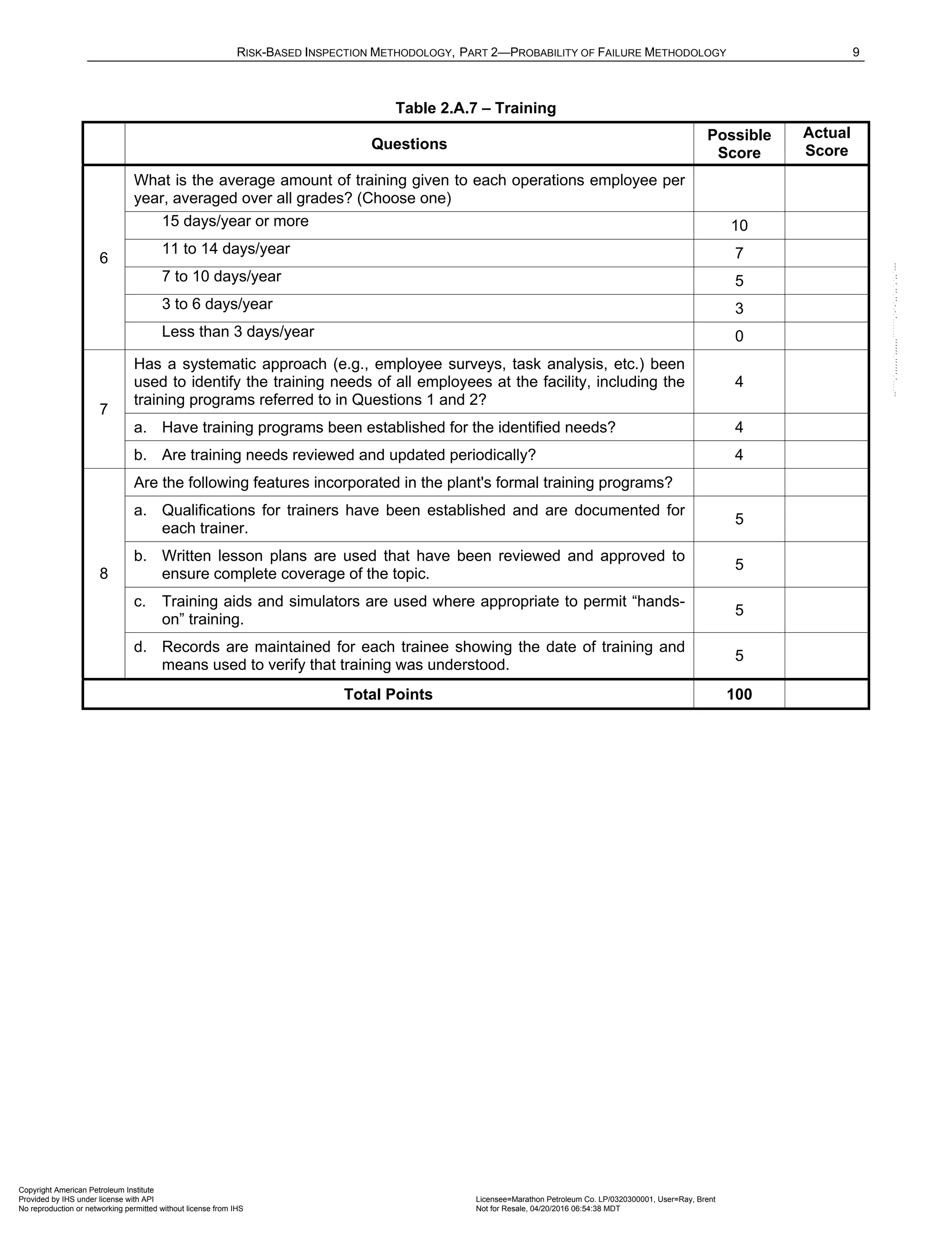
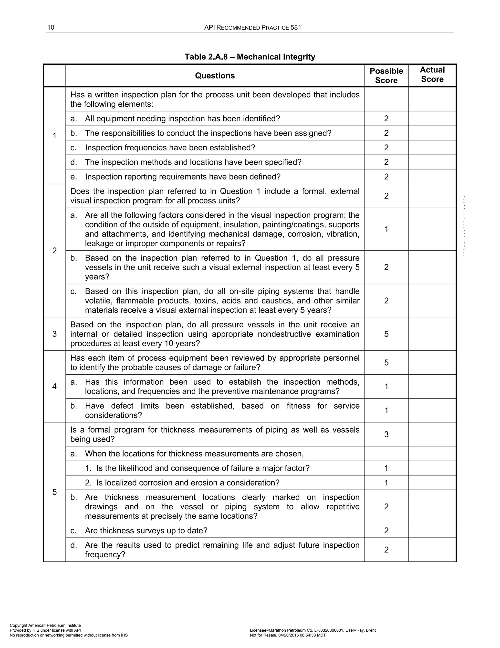
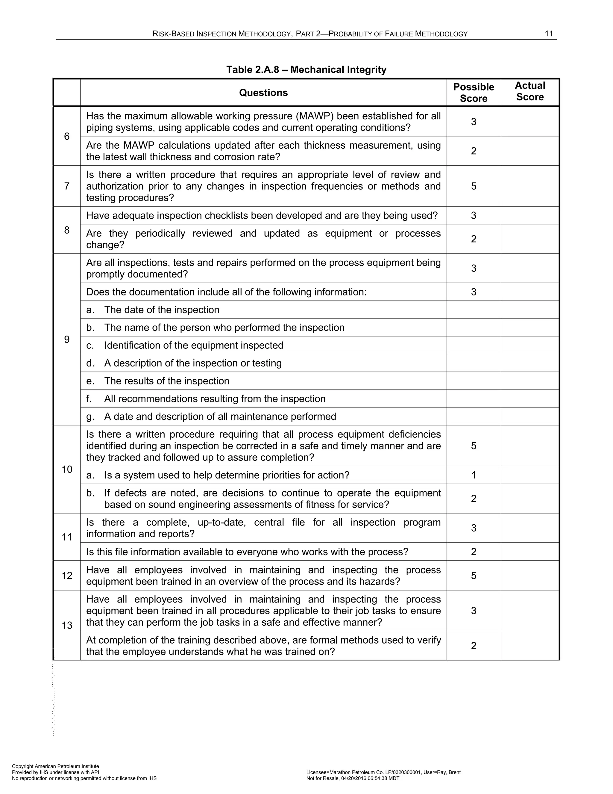
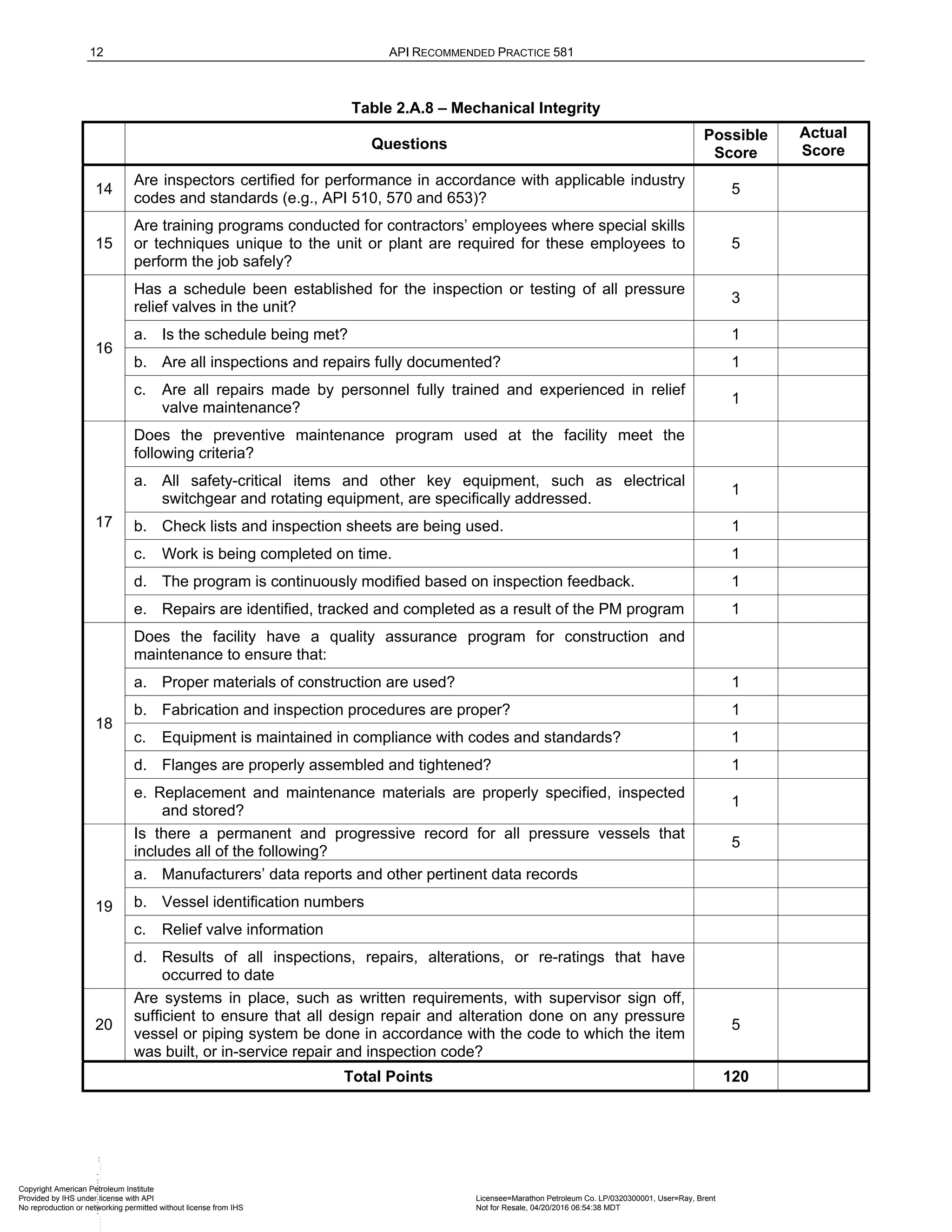
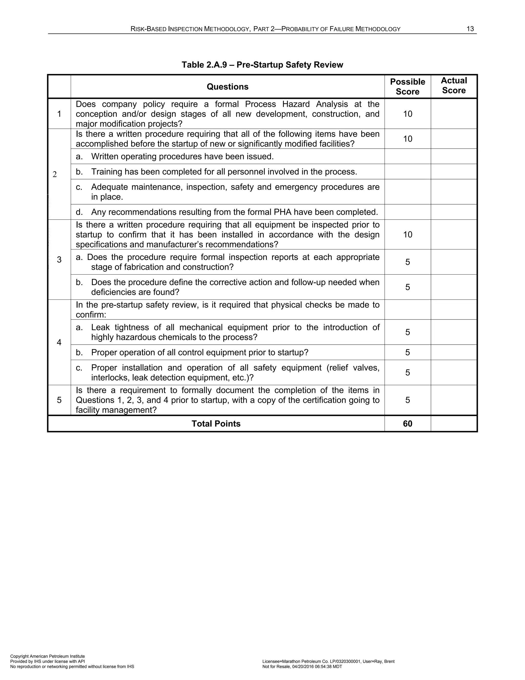

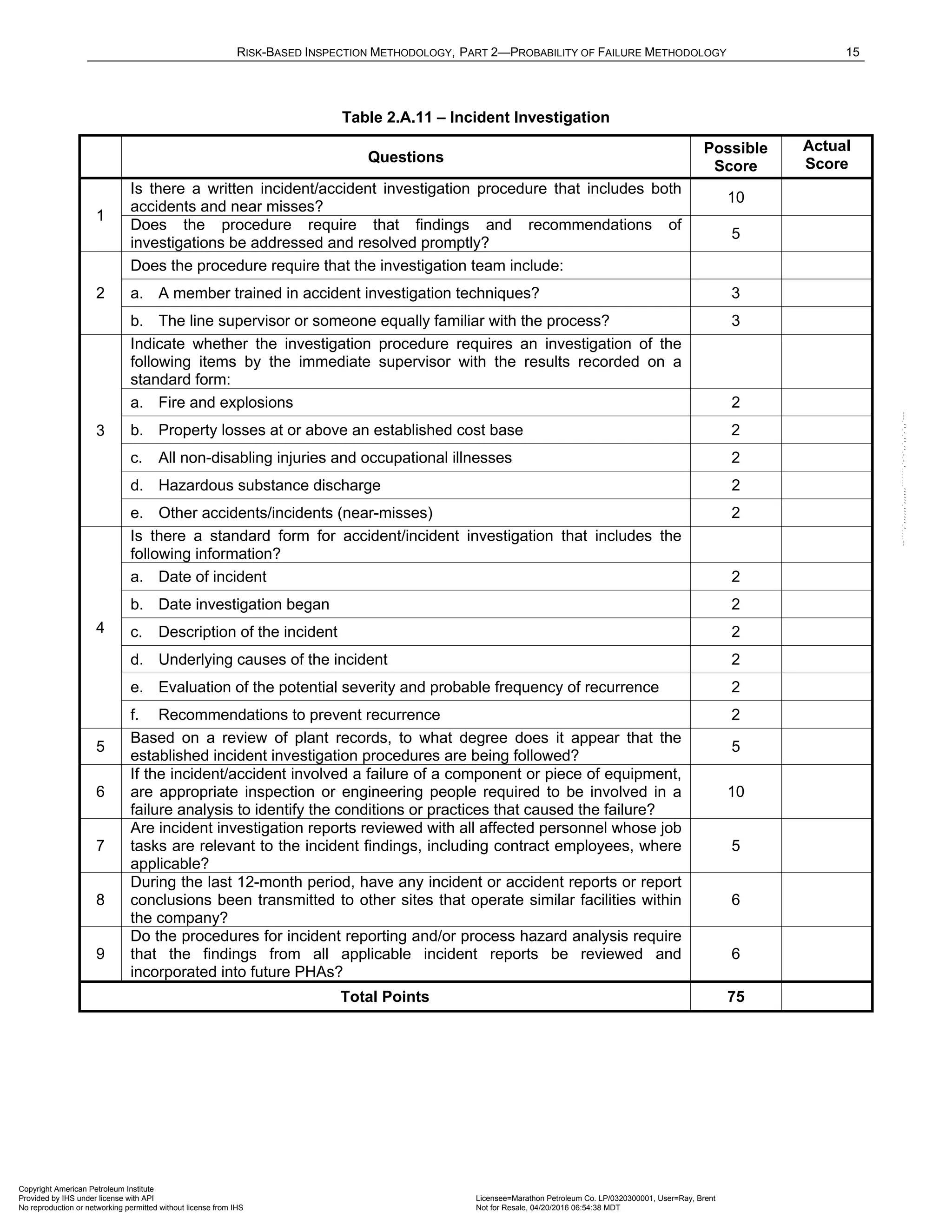
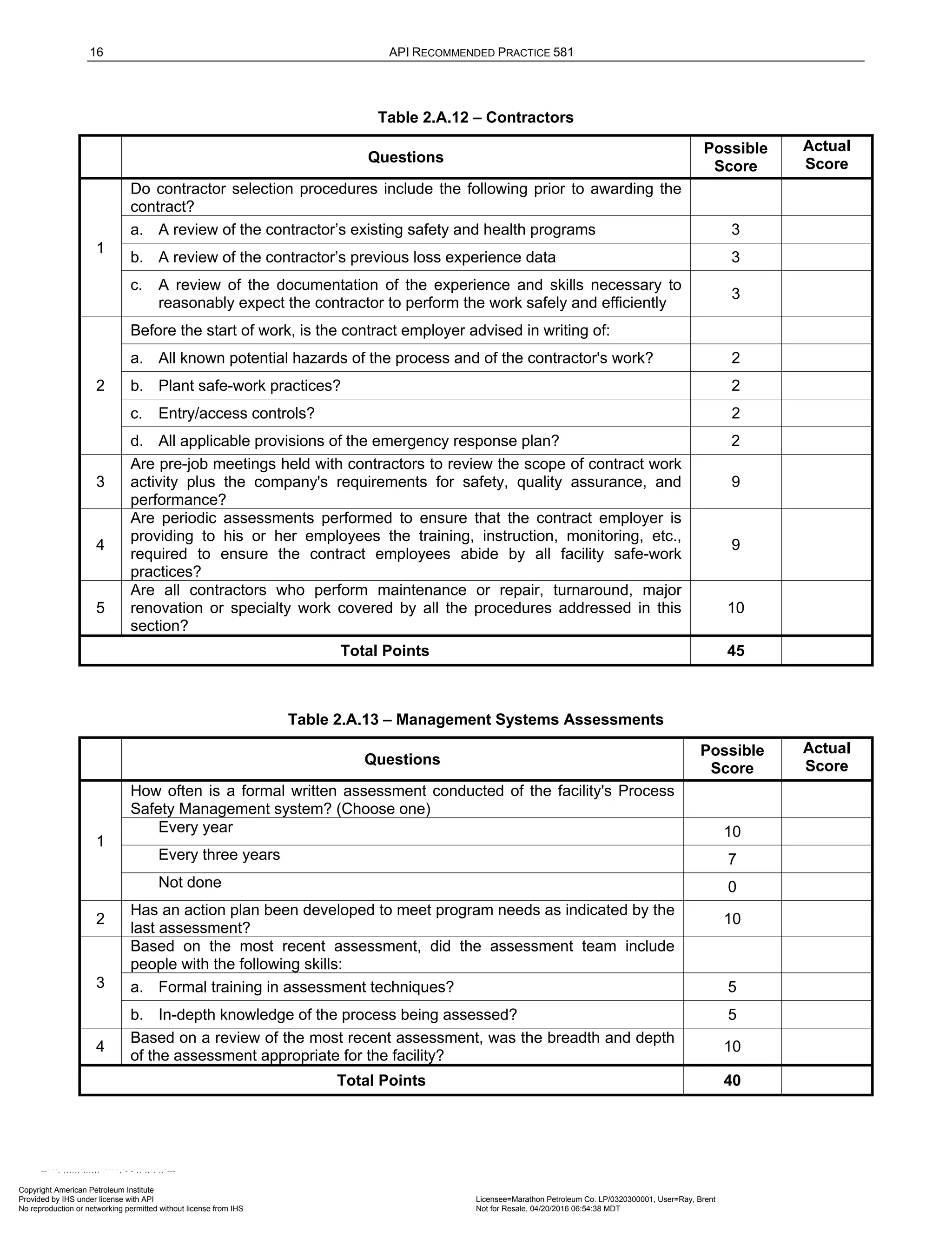

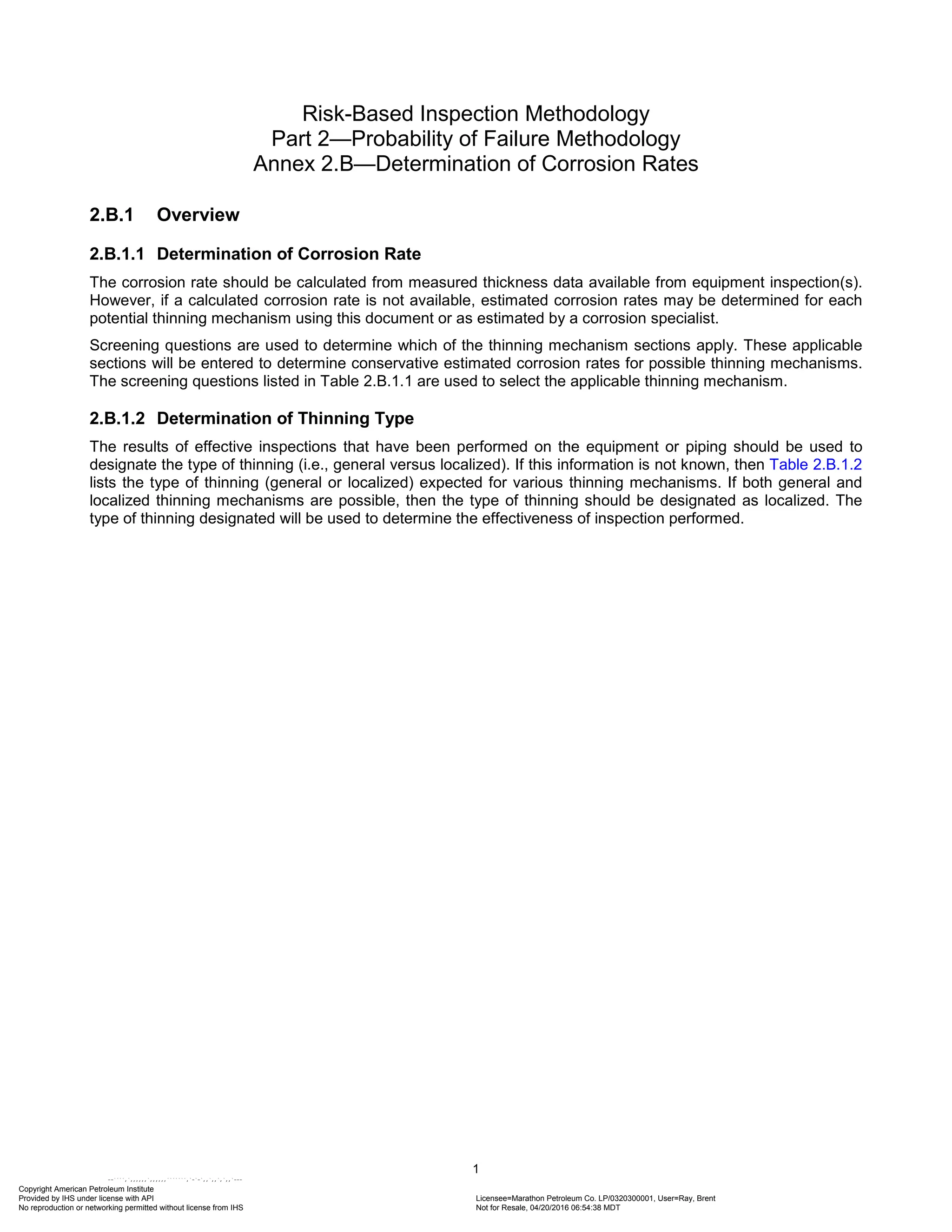
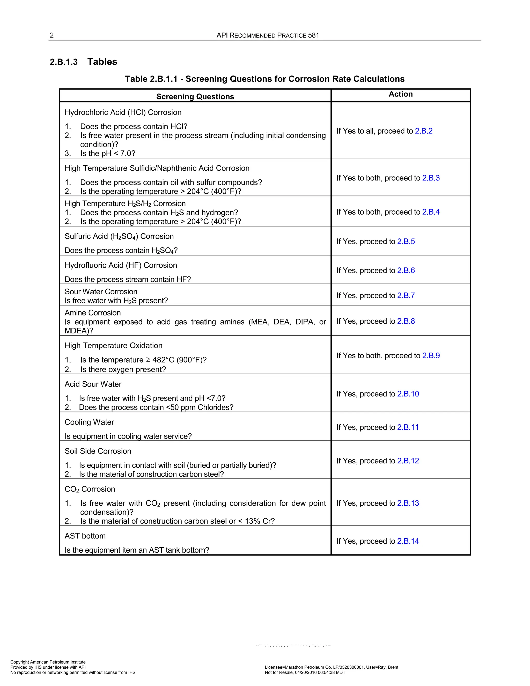
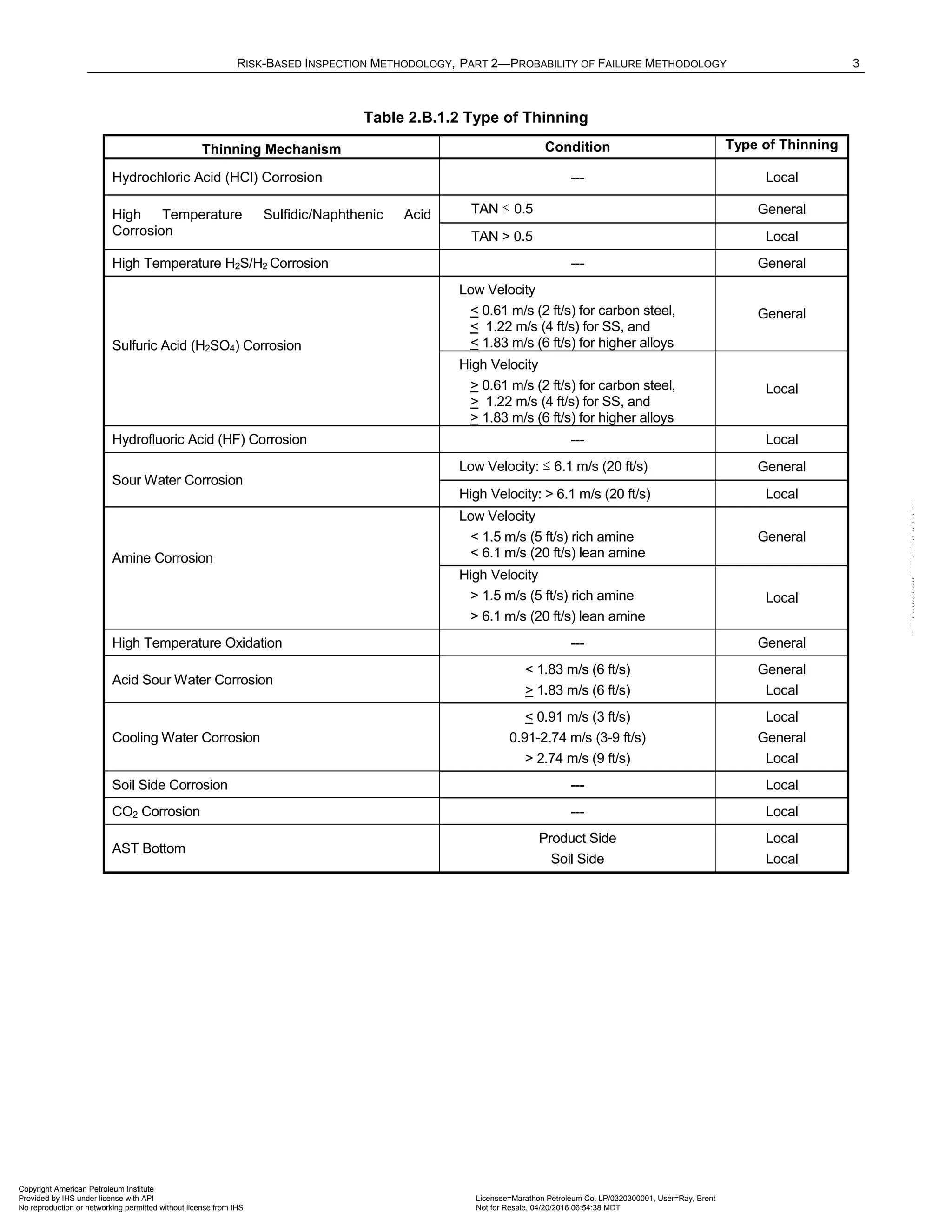
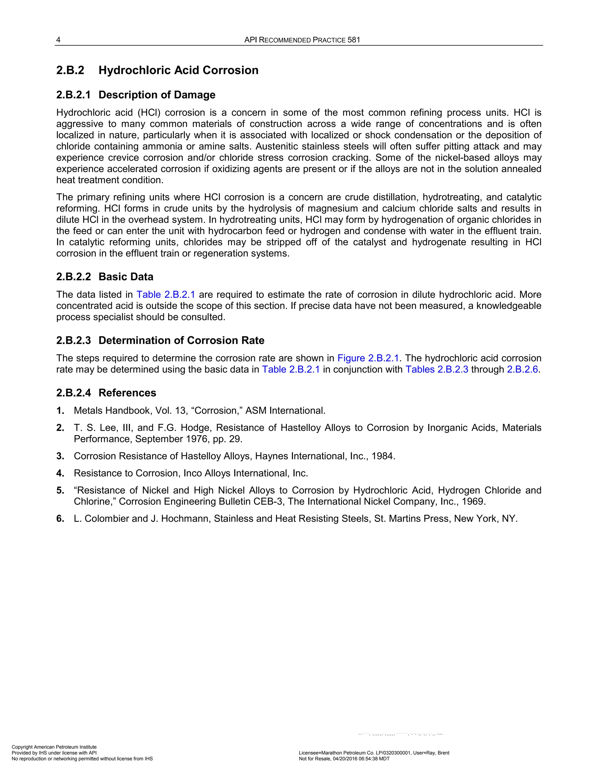
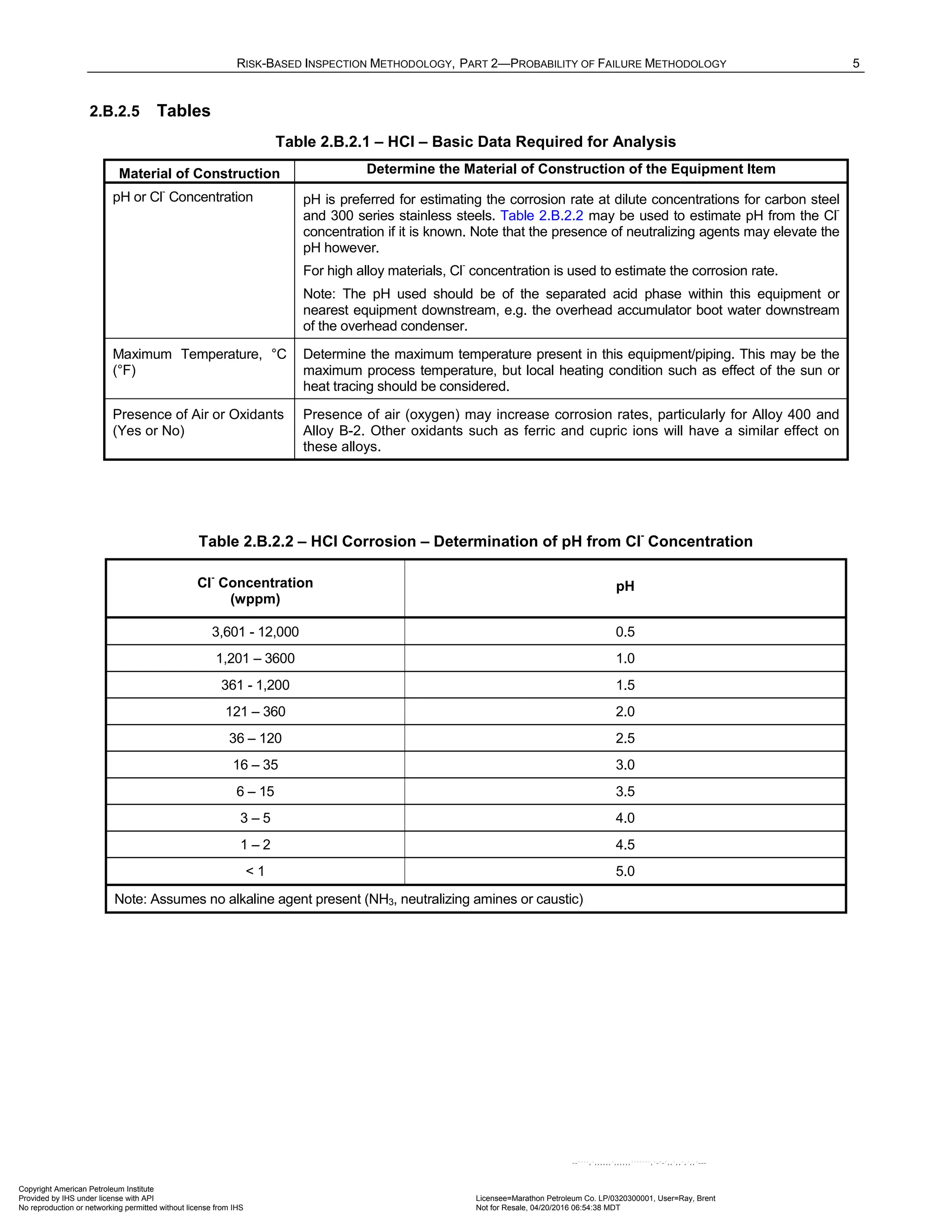
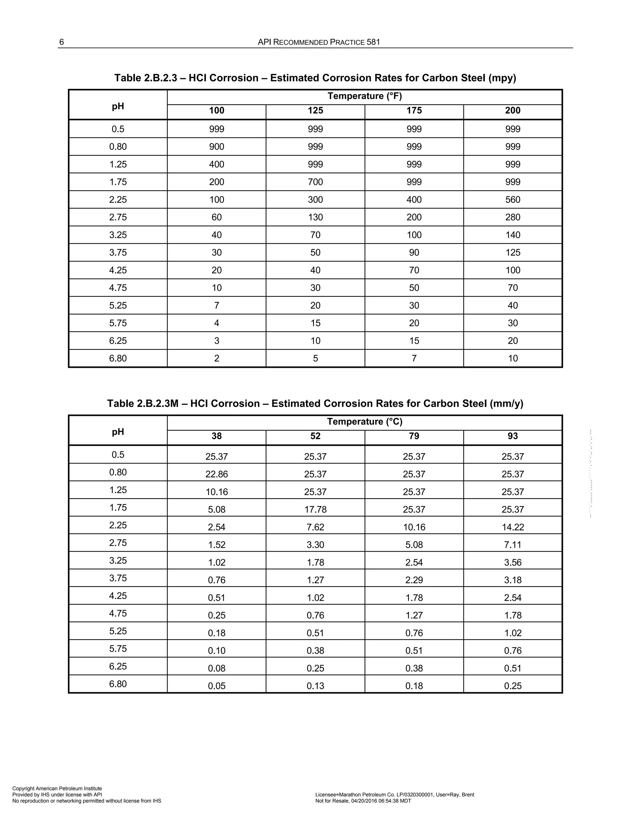
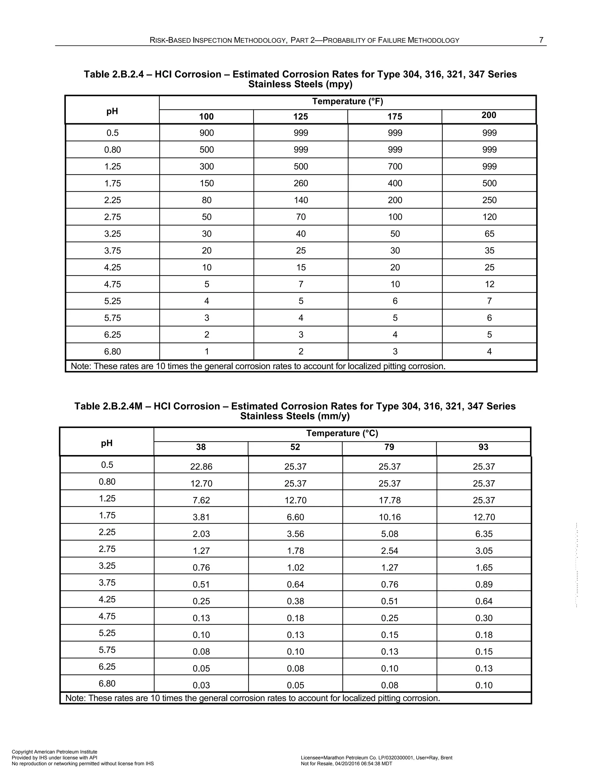
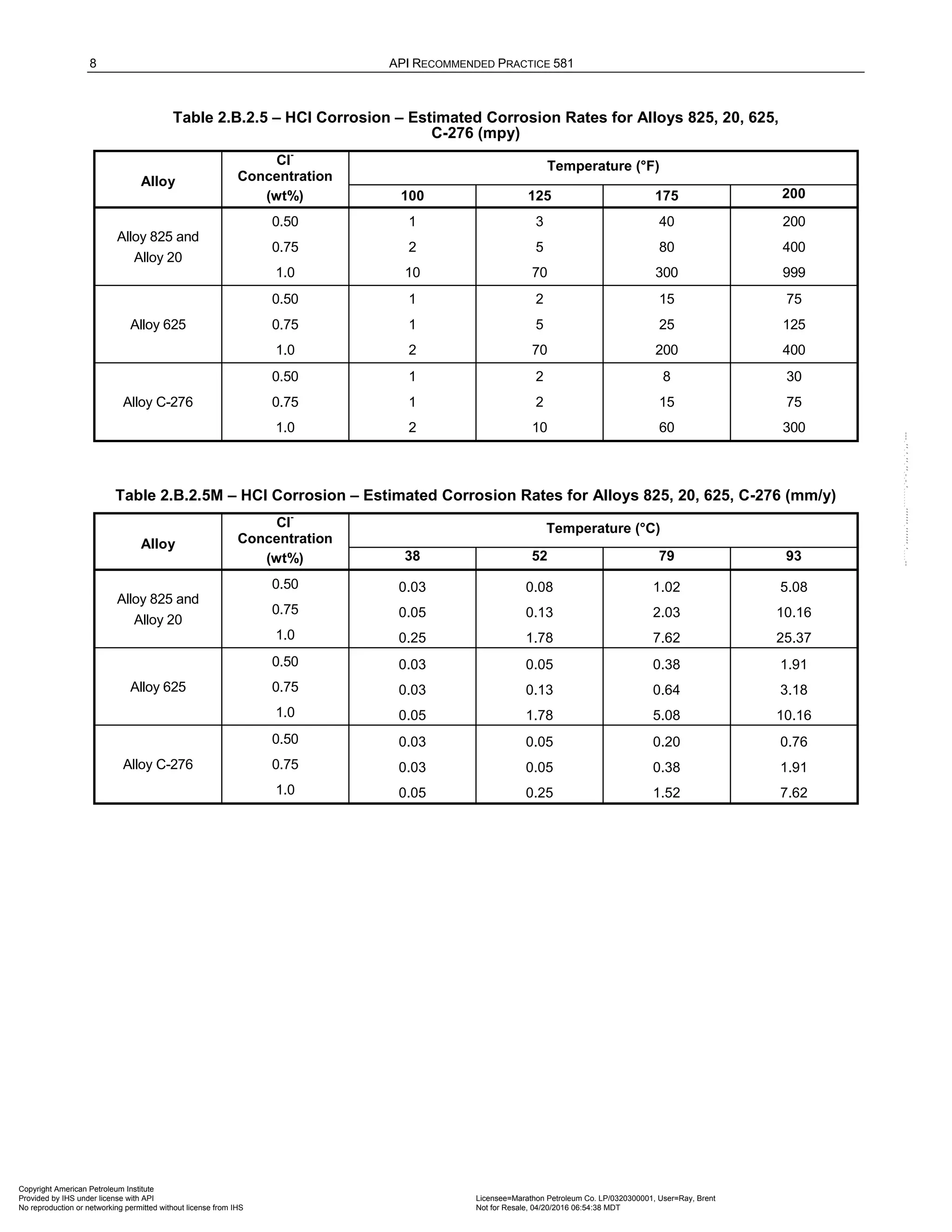
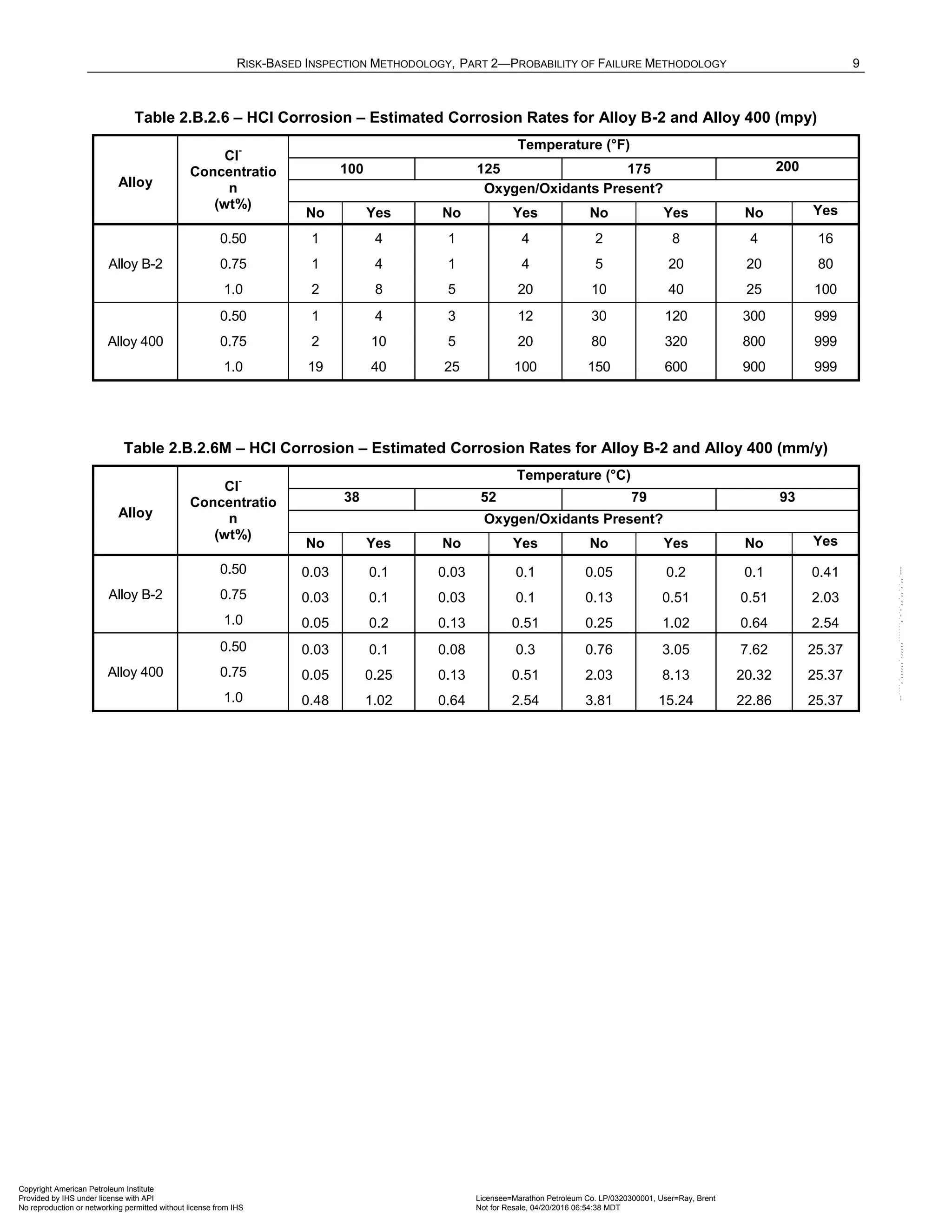
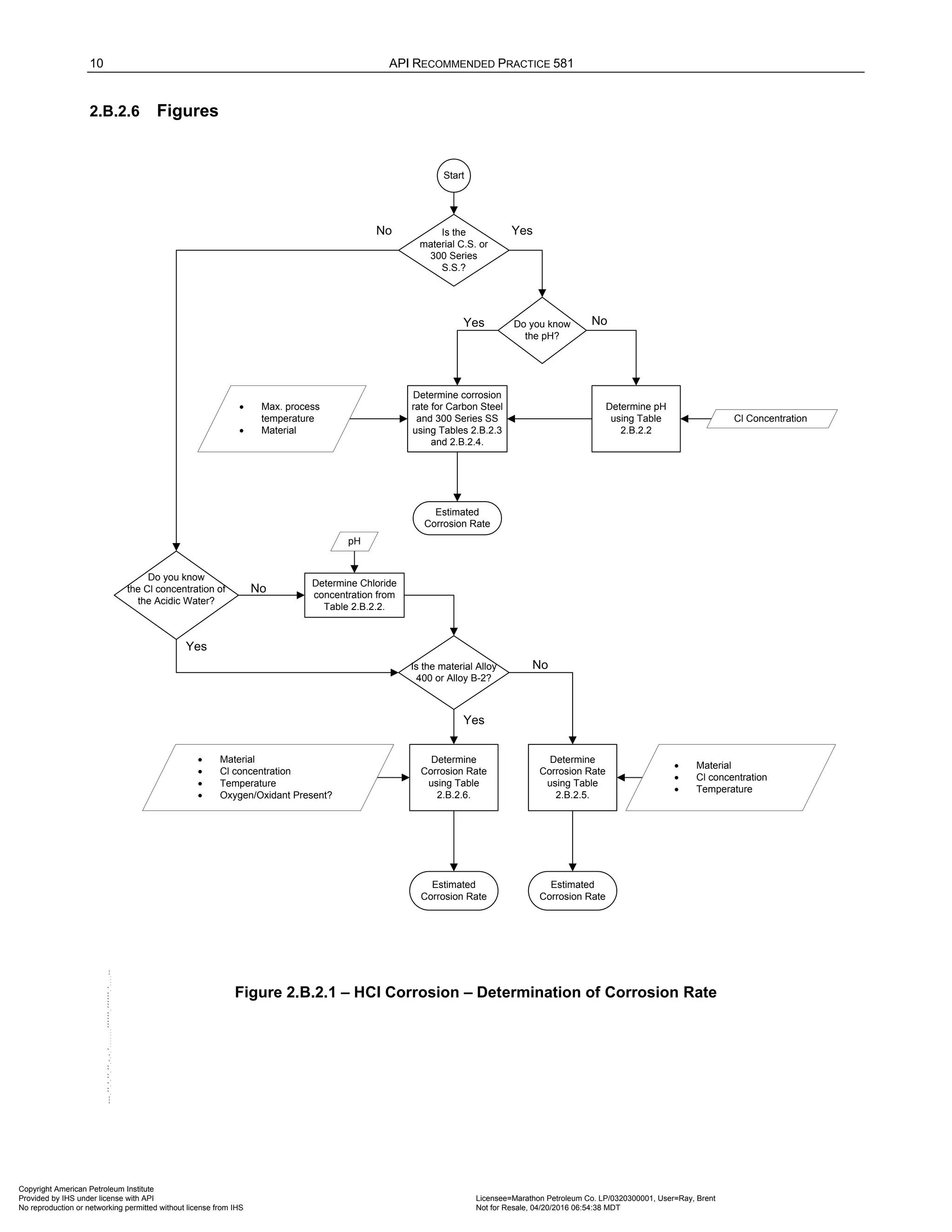
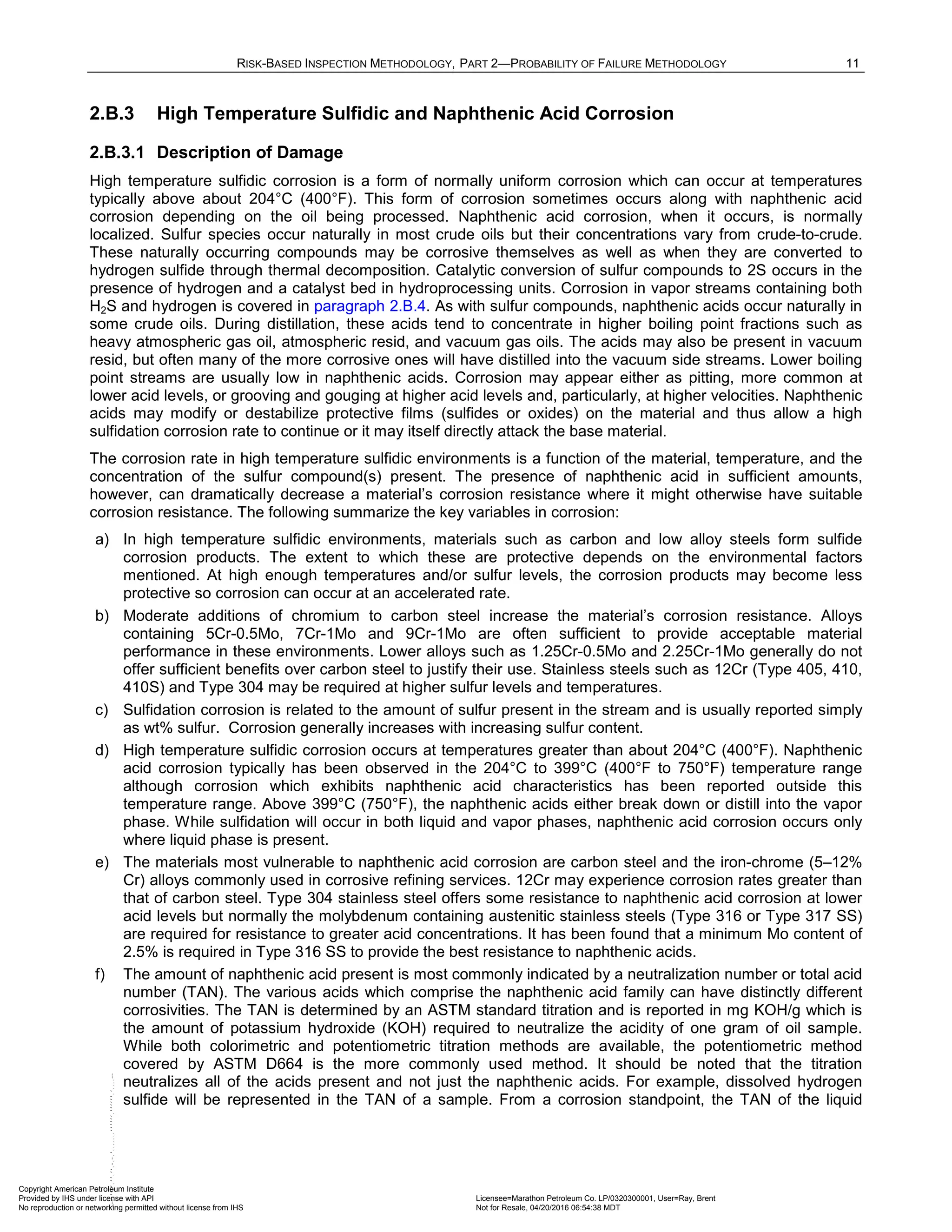
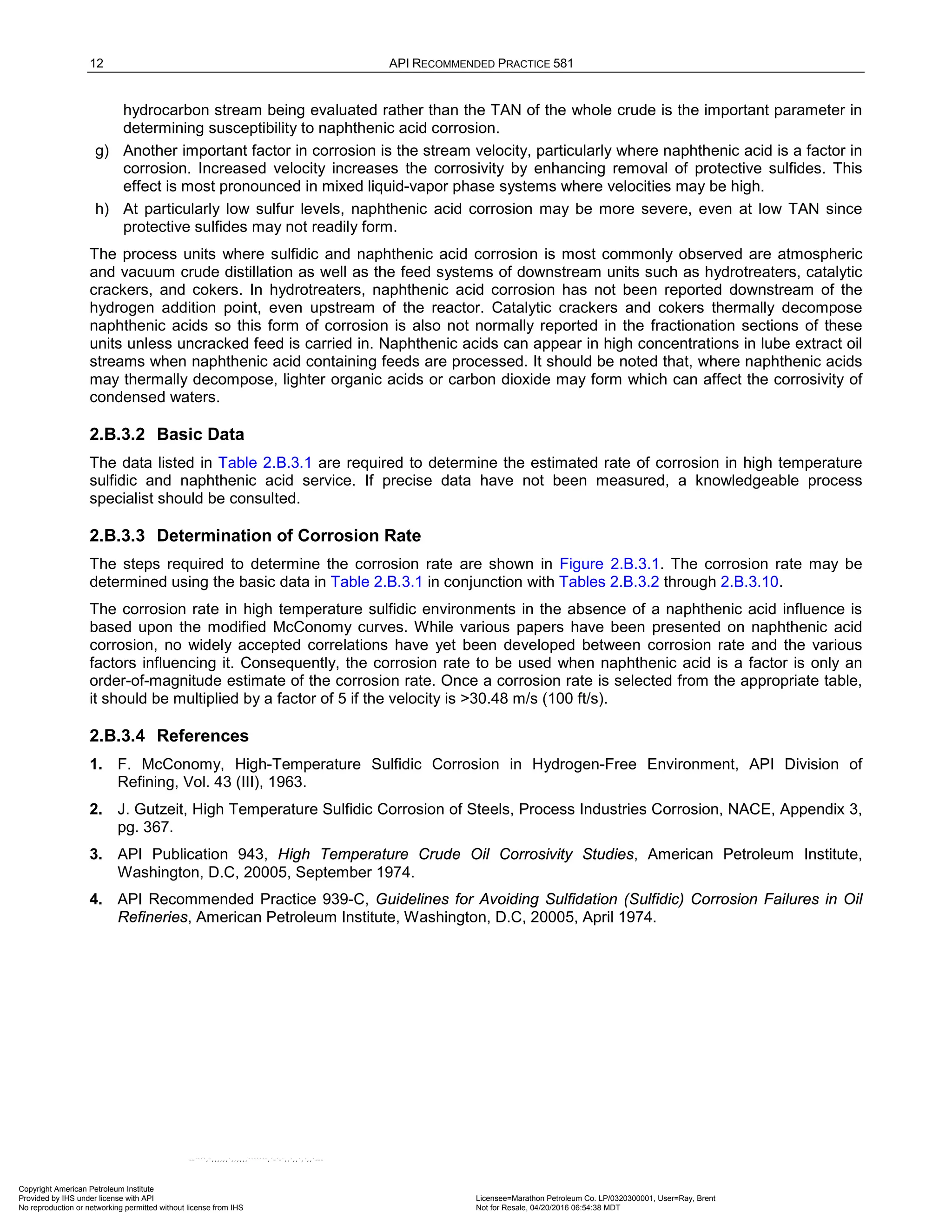
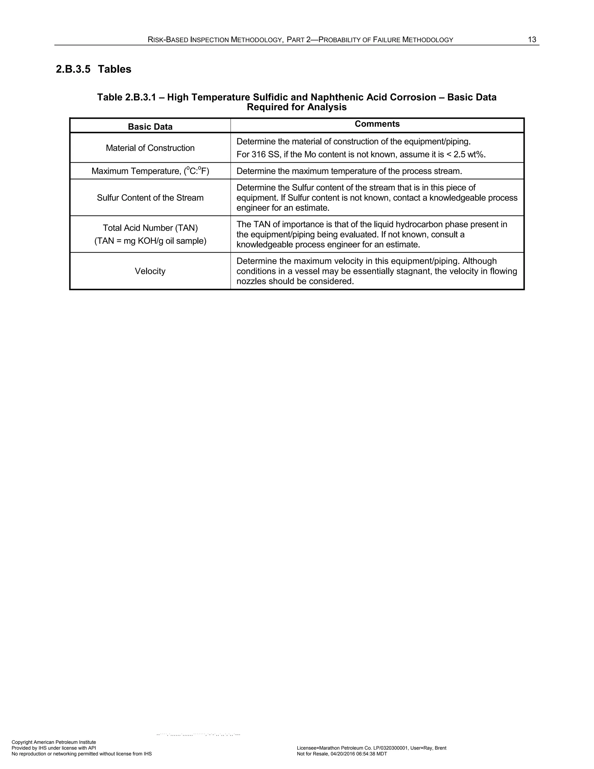
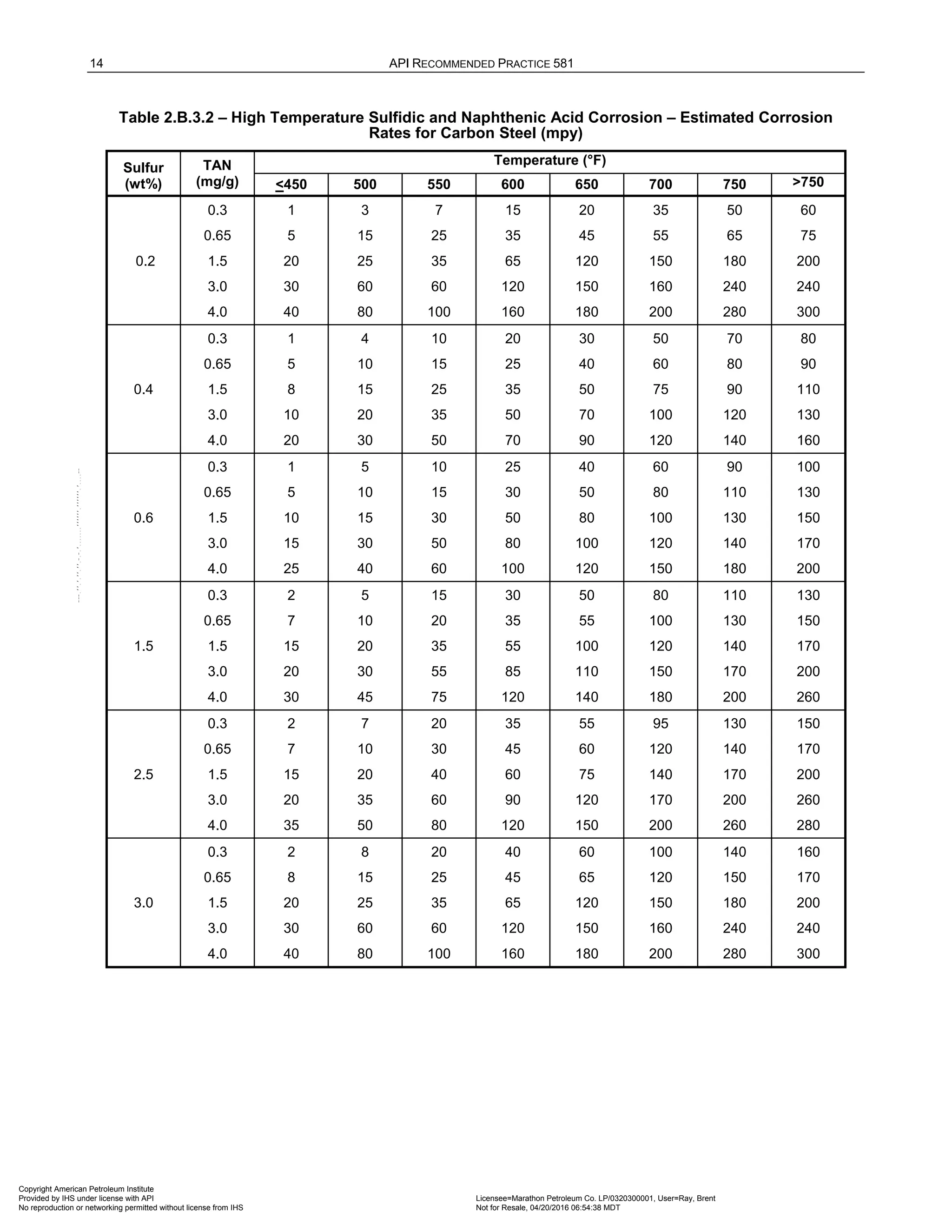

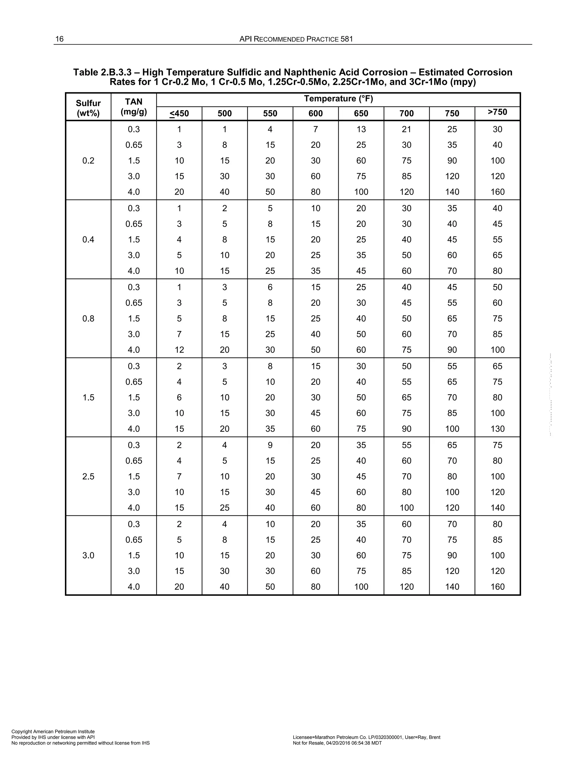
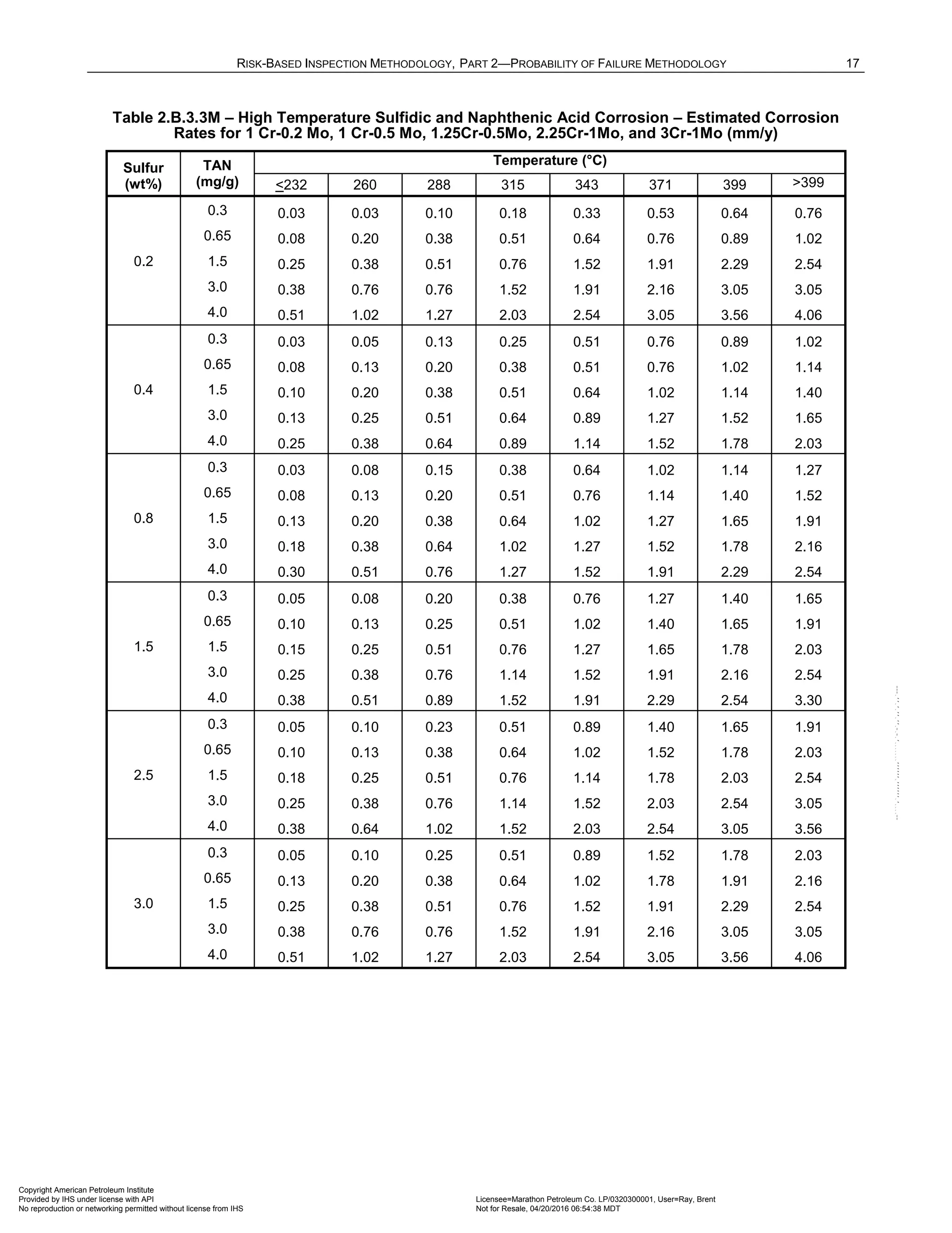
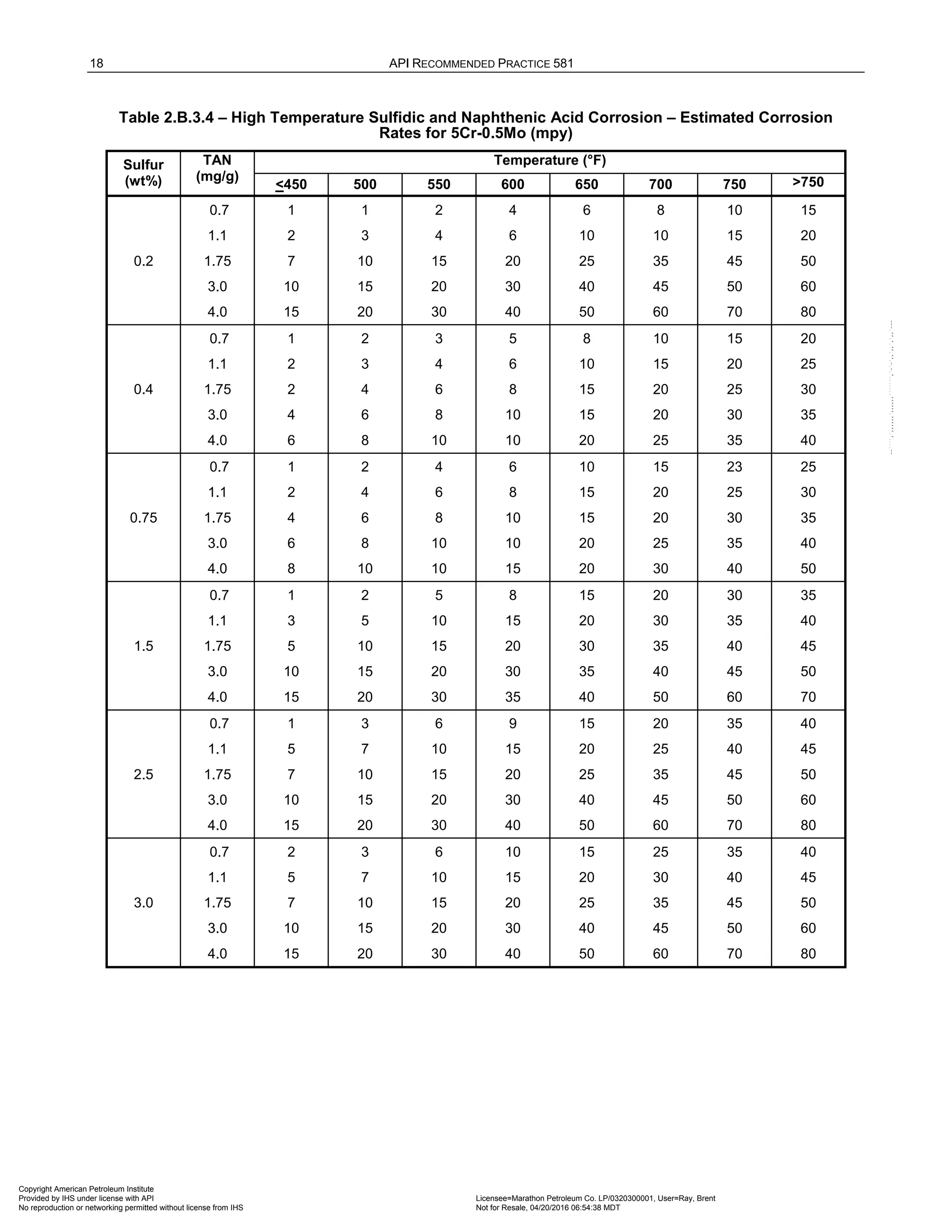
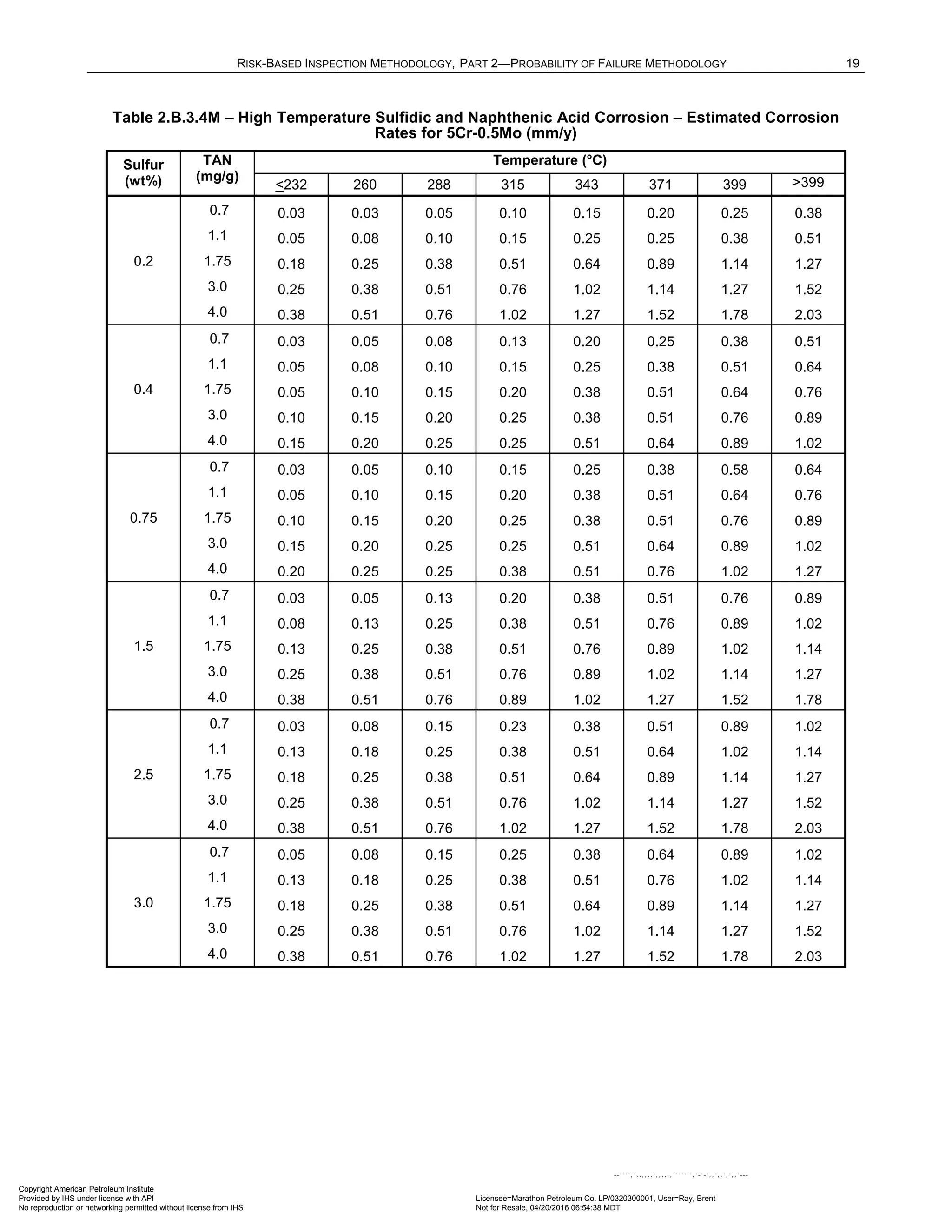
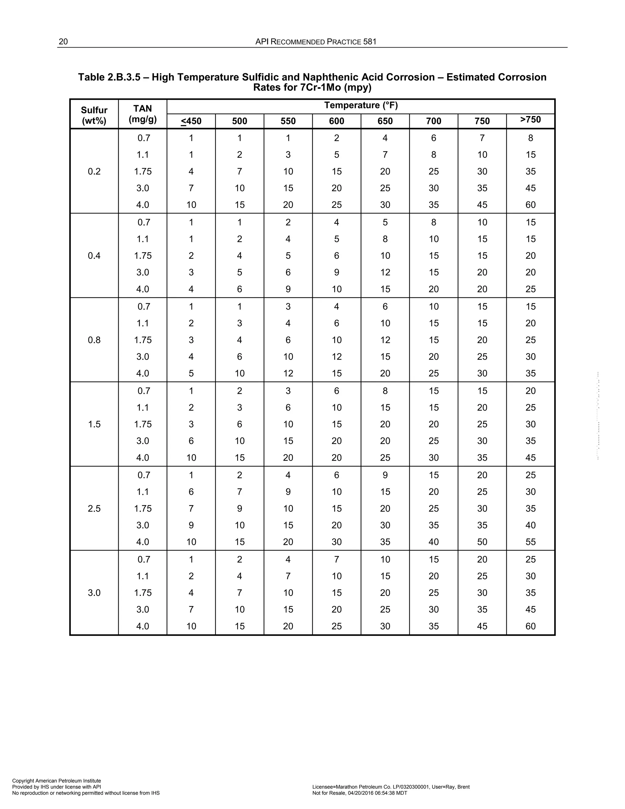

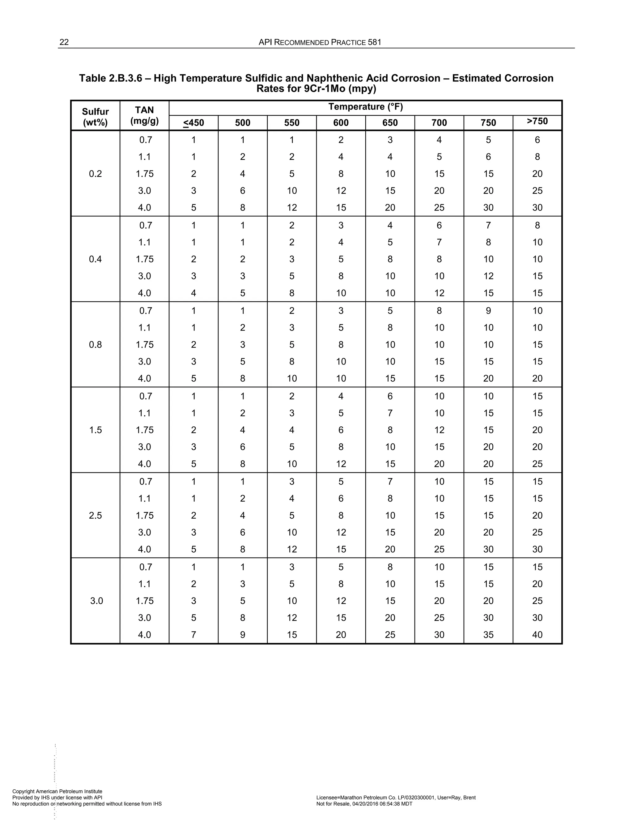

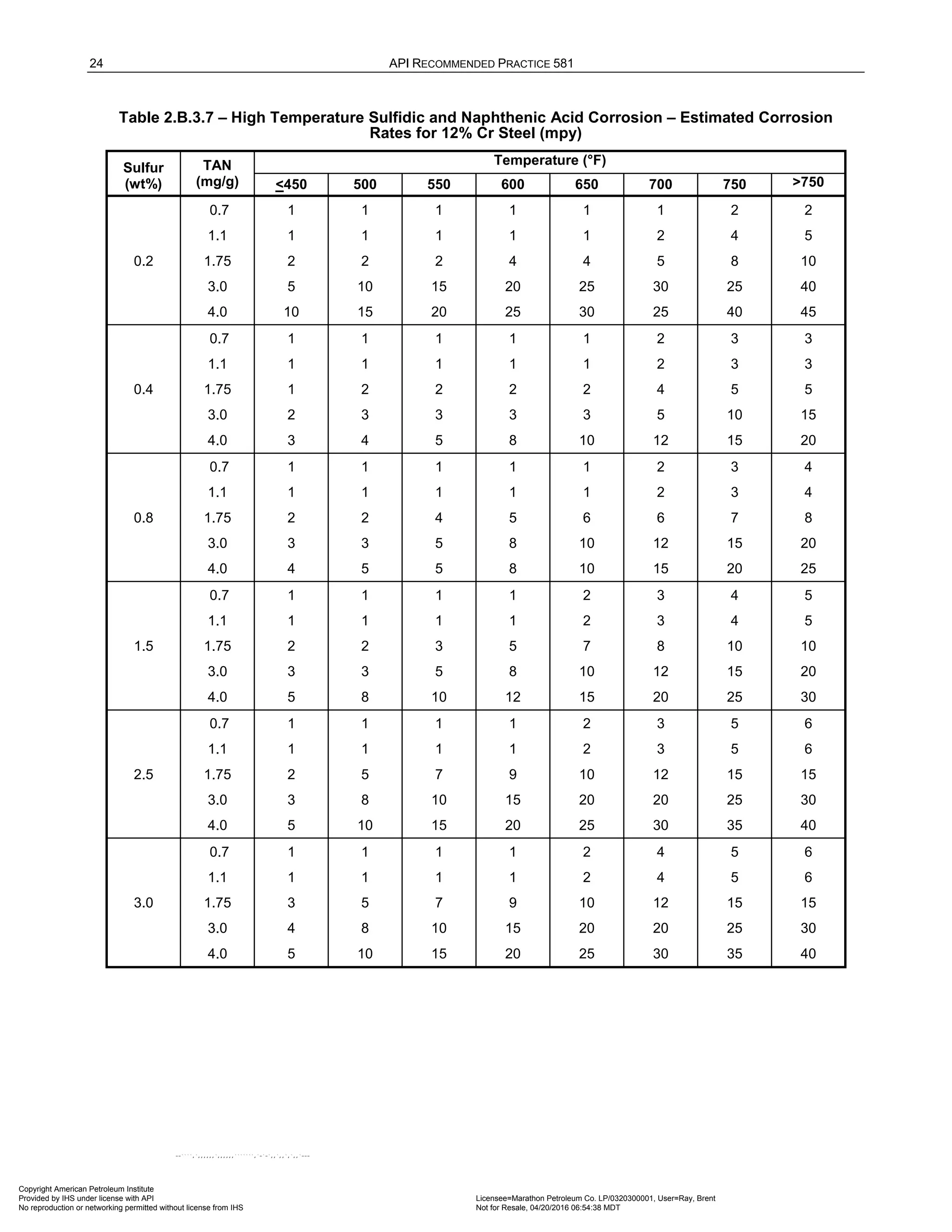
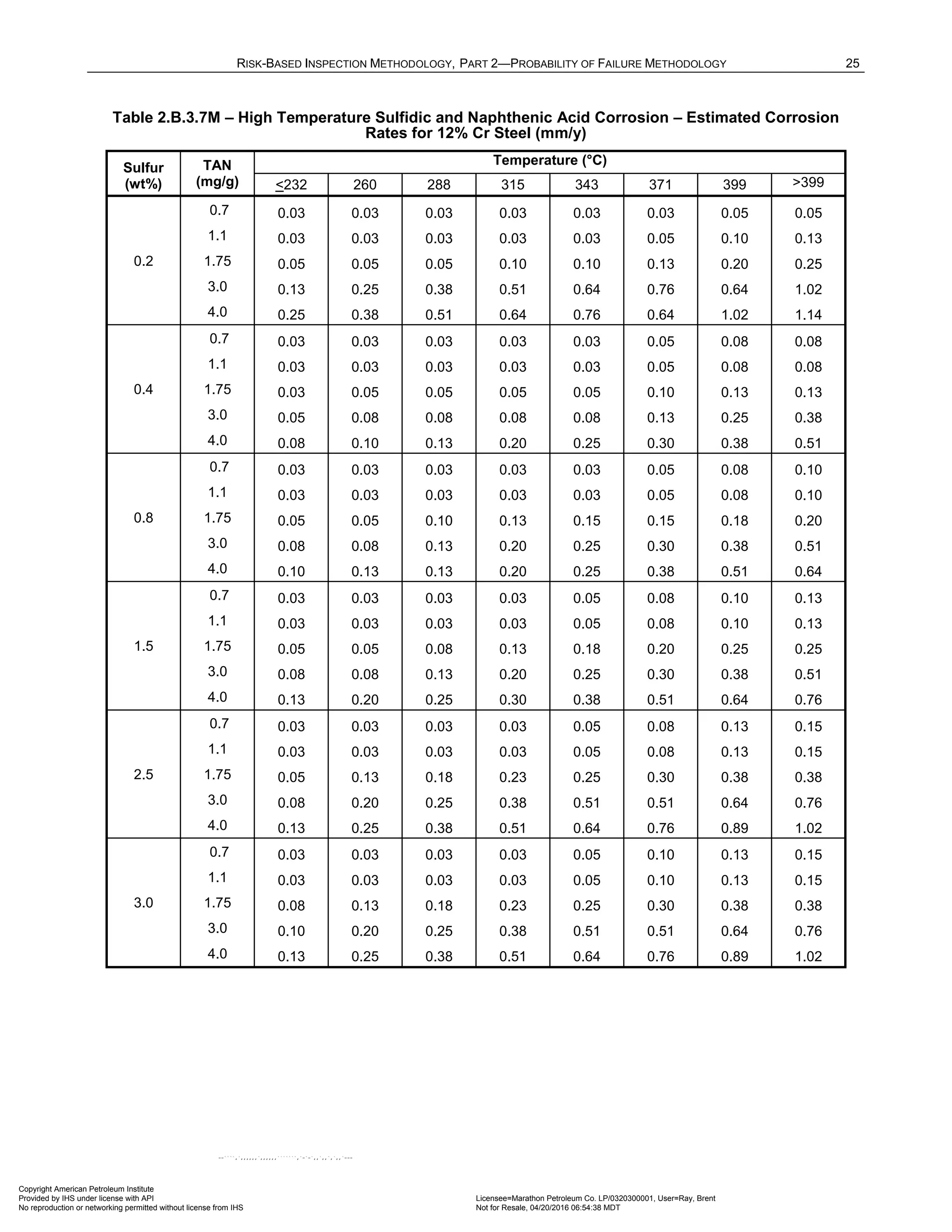
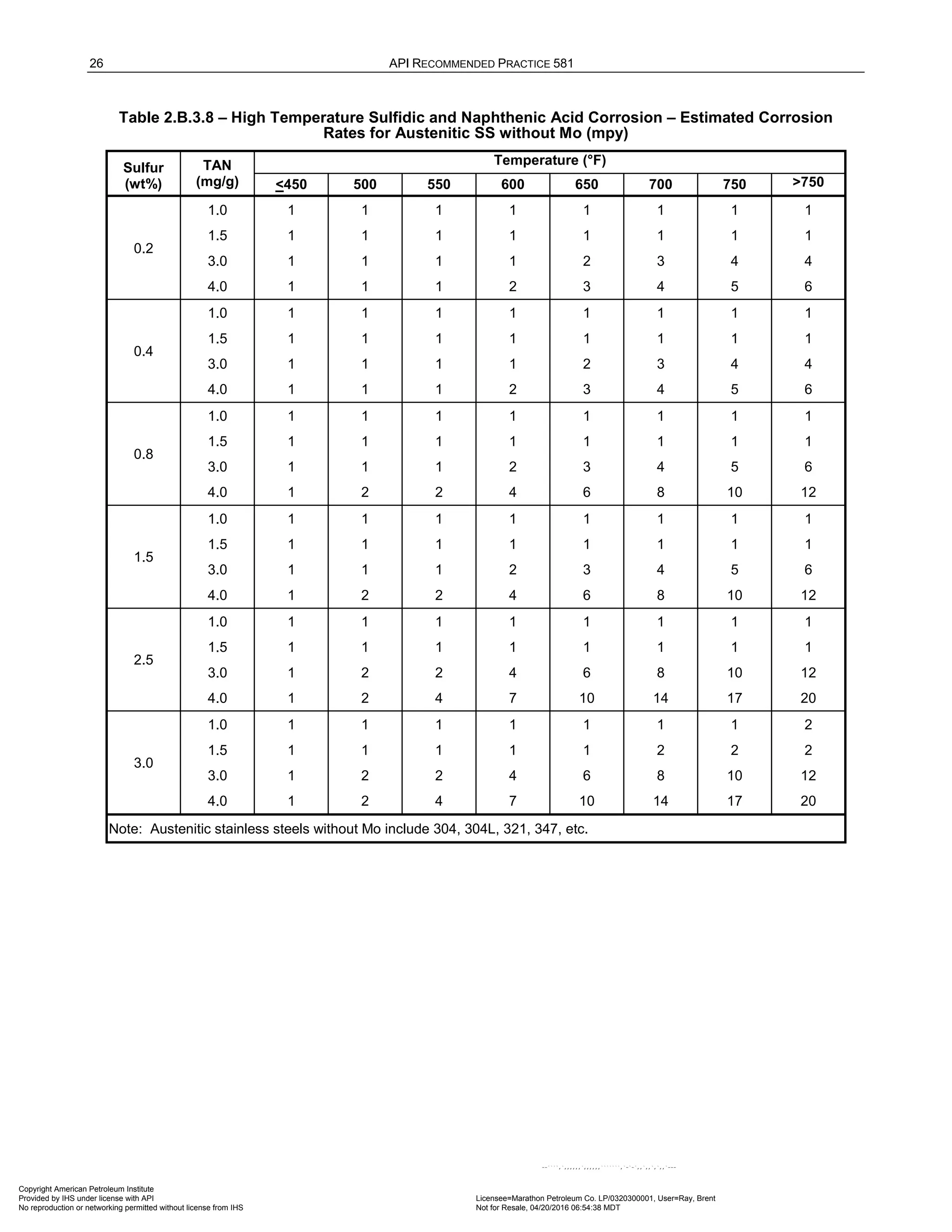
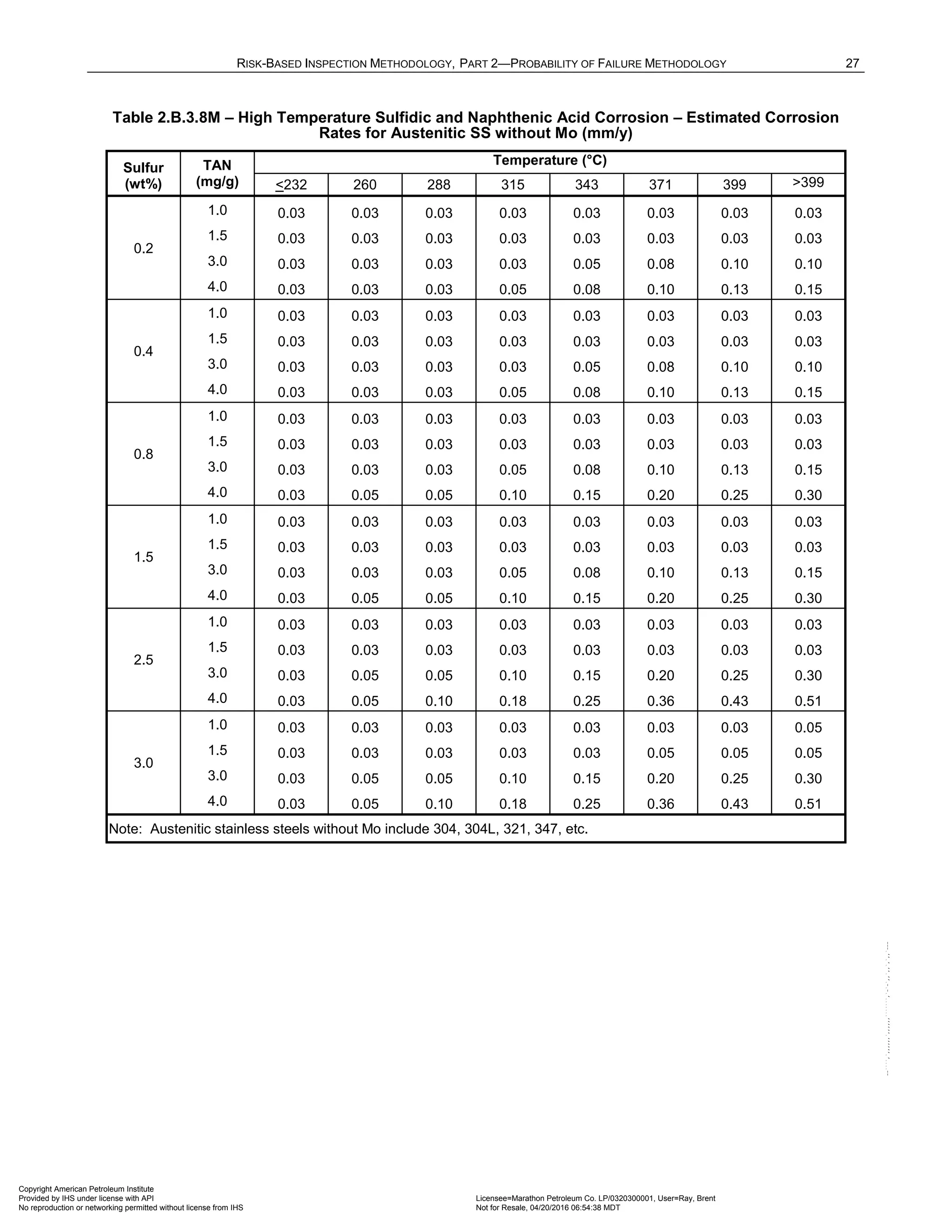
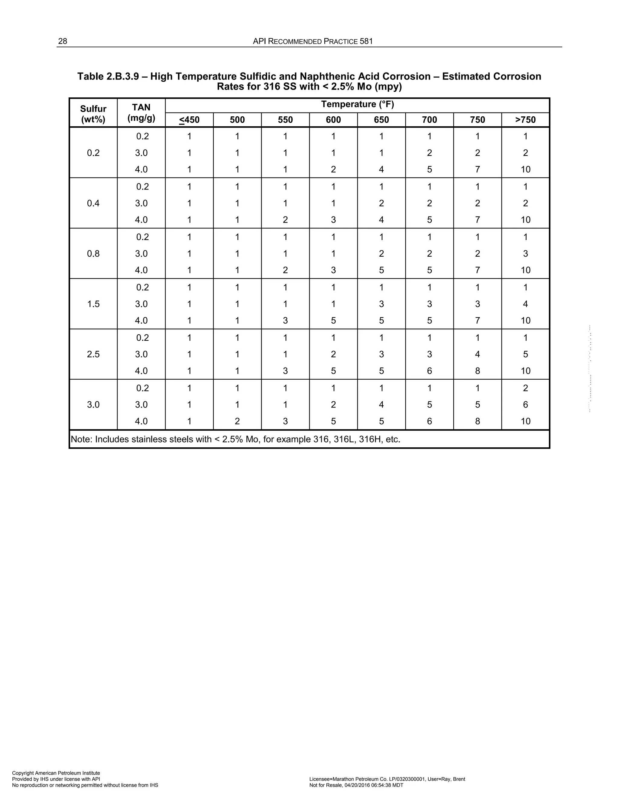
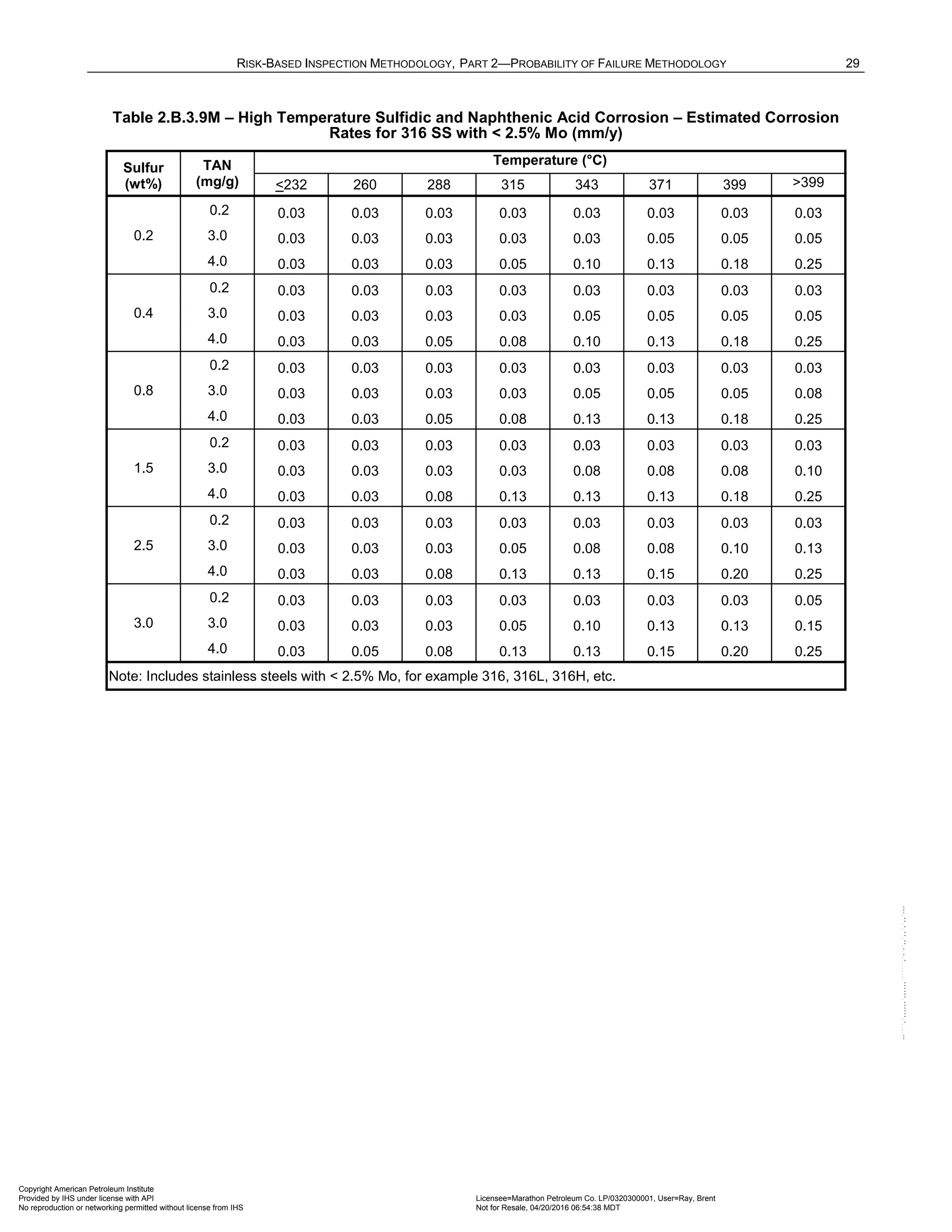
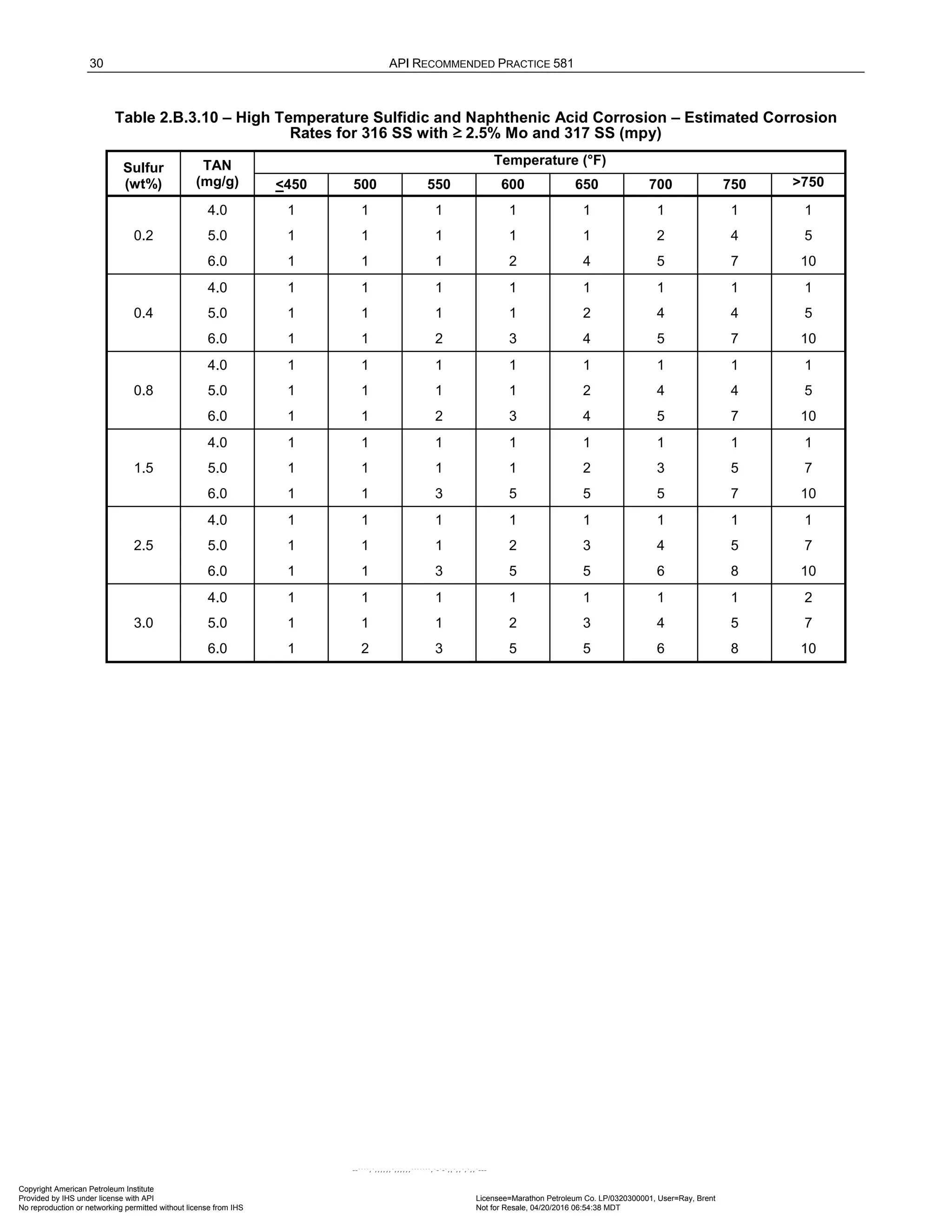
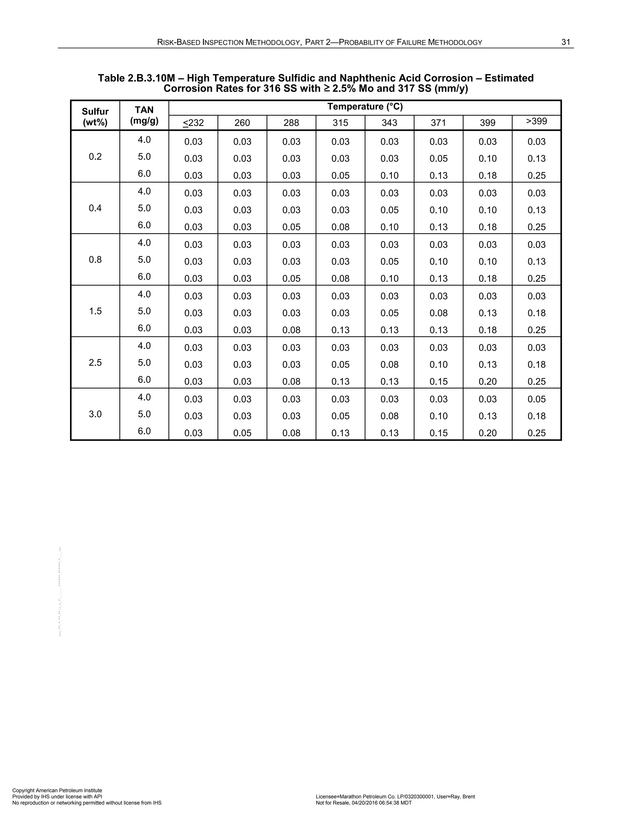
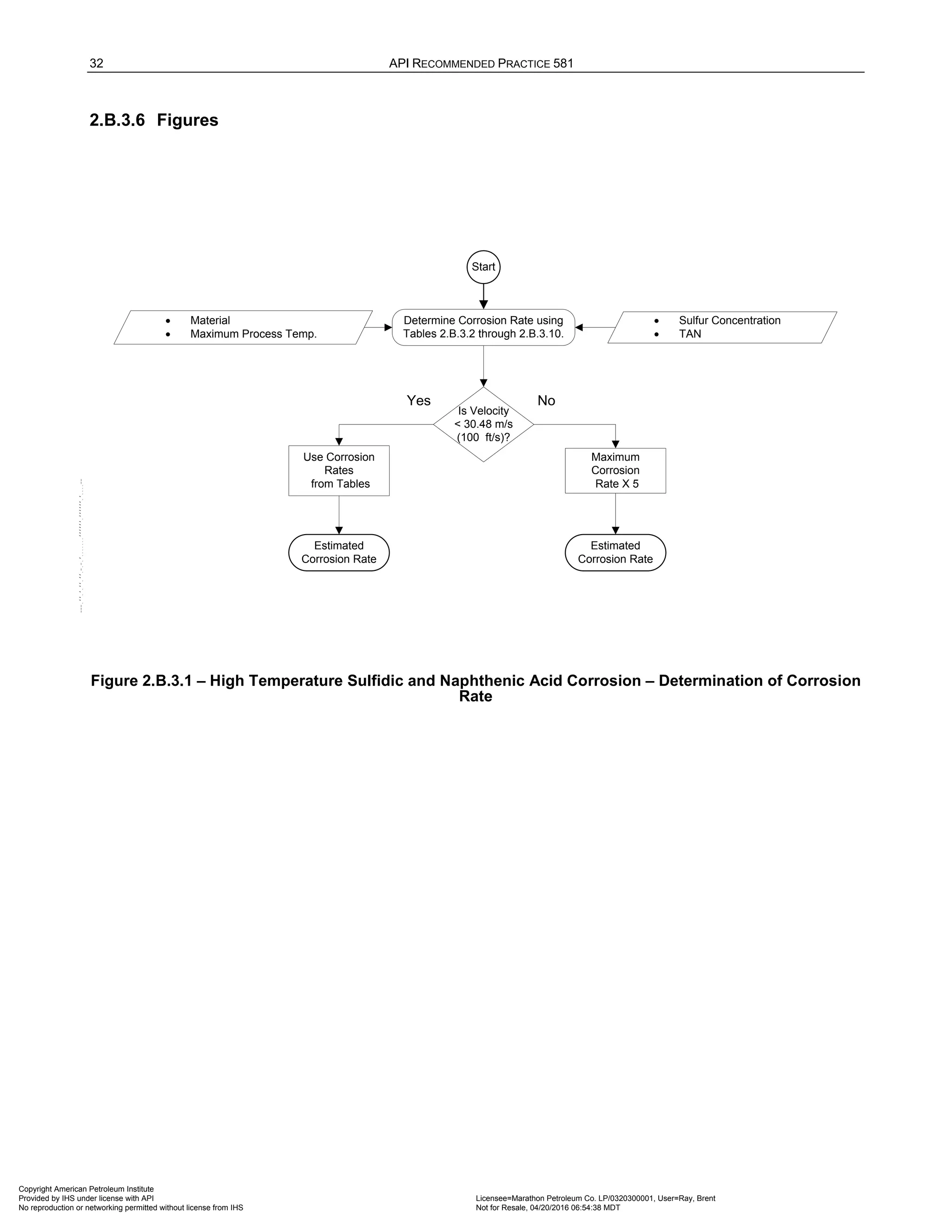
![34 API RECOMMENDED PRACTICE 581
2.B.4.5 Tables
Table 2.B.4.1 – High Temperature H2S/H2 Corrosion – Basic Data Required for Analysis
Basic Data Comments
Material of Construction Determine the material of construction of the equipment/piping.
Type of Hydrocarbon Present
(naphtha or gas oil)
The Couper-Gorman corrosion rate curves are dependent on the type of
hydrocarbon stream present [3, 4]. There are two categories as follows:
1) Naphtha refers to those hydrocarbon streams of both light and heavy
naphtha as well as light distillates (streams typically boiling at <430°F);
2) Gas Oil refers to those hydrocarbon streams that include distillate,
atmospheric gas oils, resid, and other heavier process hydrocarbons (streams
typically boiling at >430°F).
Maximum Temperature (
o
C:°F) Determine the maximum process temperature.
H2S Content of the Vapor
(mole %)
Determine the H2S content in the vapor.
Note that mole% = volume % (not wt%)
Table 2.B.4.2 – High Temperature H2S/H2 Corrosion – Estimated Corrosion Rates for Carbon Steel,
1 Cr-0.2 Mo, 1 Cr-0.5 Mo, 1.25Cr-0.5Mo, 2.25Cr-1Mo, and 3Cr-1Mo (mpy)
H2S
(mole %)
Type of
Hydrocarbon
Temperature (°F)
425 475 525 575 625 675 725 775 825 875 925 975
0.002
Naphtha 1 1 1 1 2 3 4 6 8 10 14 18
Gas Oil 1 1 1 2 3 5 7 10 14 20 26 34
0.0035
Naphtha 1 1 1 2 4 6 8 12 16 22 29 37
Gas Oil 1 2 3 4 7 11 16 22 31 41 55 71
0.008
Naphtha 1 1 2 3 5 7 11 15 21 29 38 50
Gas Oil 1 2 4 6 9 14 21 29 41 55 73 94
0.035
Naphtha 1 2 3 5 9 13 19 27 38 51 67 87
Gas Oil 2 4 6 10 16 25 36 51 71 96 130 170
0.08
Naphtha 1 2 4 7 10 16 23 33 46 62 82 110
Gas Oil 2 4 8 13 20 30 44 63 87 120 160 200
0.30
Naphtha 2 3 6 10 15 23 34 48 66 90 120 150
Gas Oil 3 6 11 18 29 44 64 91 130 170 230 300
0.75
Naphtha 2 4 7 11 17 26 38 54 75 100 130 170
Gas Oil 4 7 12 21 32 49 72 100 140 190 250 330
1.0
Naphtha 3 5 8 13 21 32 47 67 93 130 170 220
Gas Oil 5 9 15 26 40 61 89 130 180 240 310 410
Copyright American Petroleum Institute
Provided by IHS under license with API Licensee=Marathon Petroleum Co. LP/0320300001, User=Ray, Brent
Not for Resale, 04/20/2016 06:54:38 MDT
No reproduction or networking permitted without license from IHS
--````,`,,,,,,`,,,,,,```````,`-`-`,,`,,`,`,,`---](https://image.slidesharecdn.com/api581-3rdedition-april2016-240227010601-3bf73ab5/75/Norma-API-581-3rd-Edition-April-2016-pdf-344-2048.jpg)


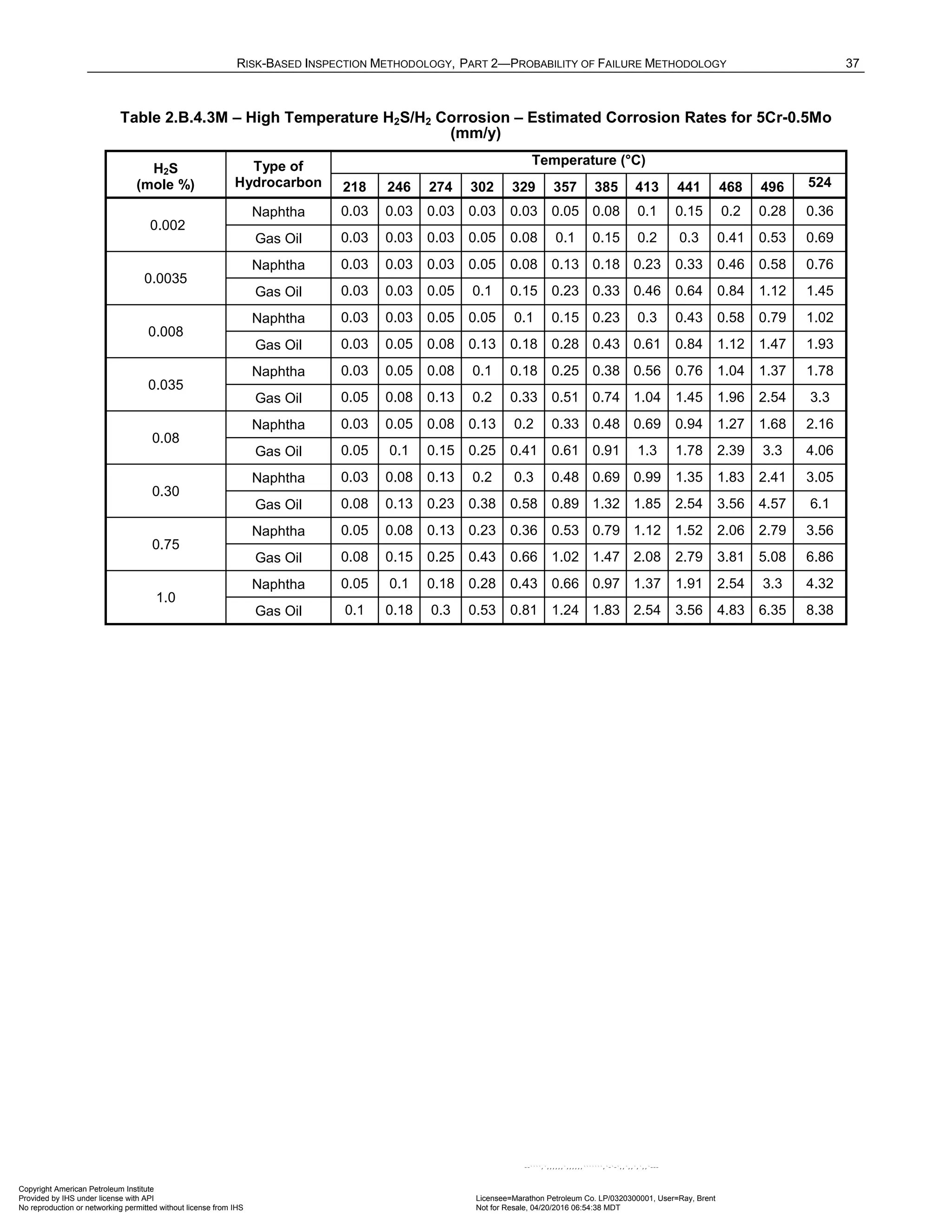

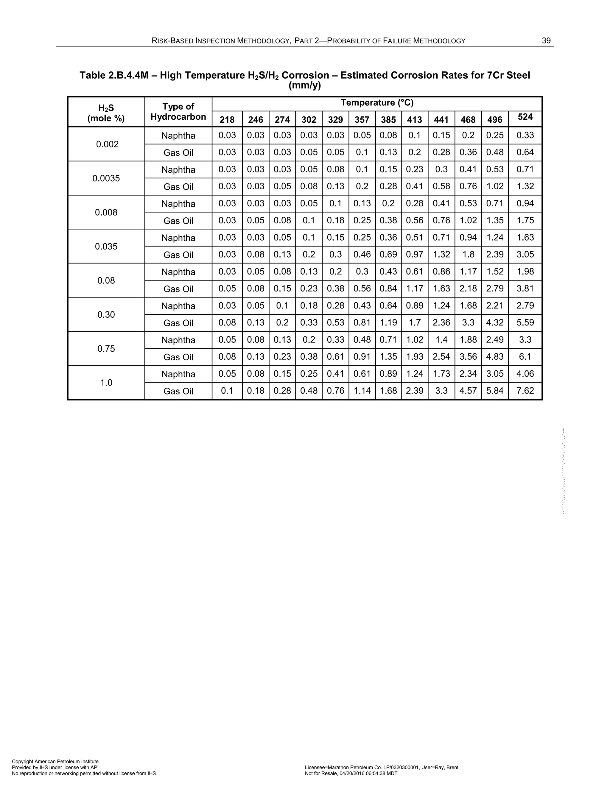
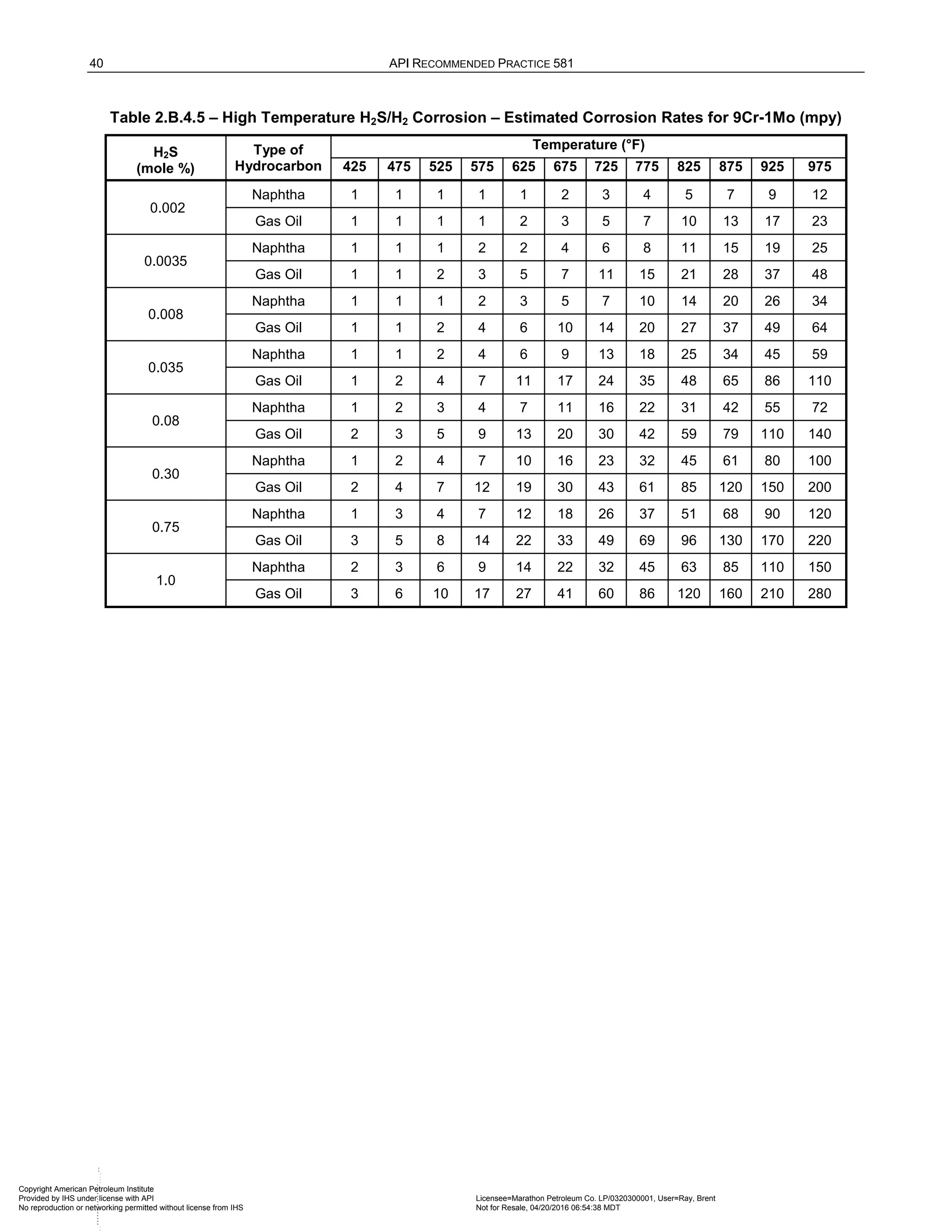
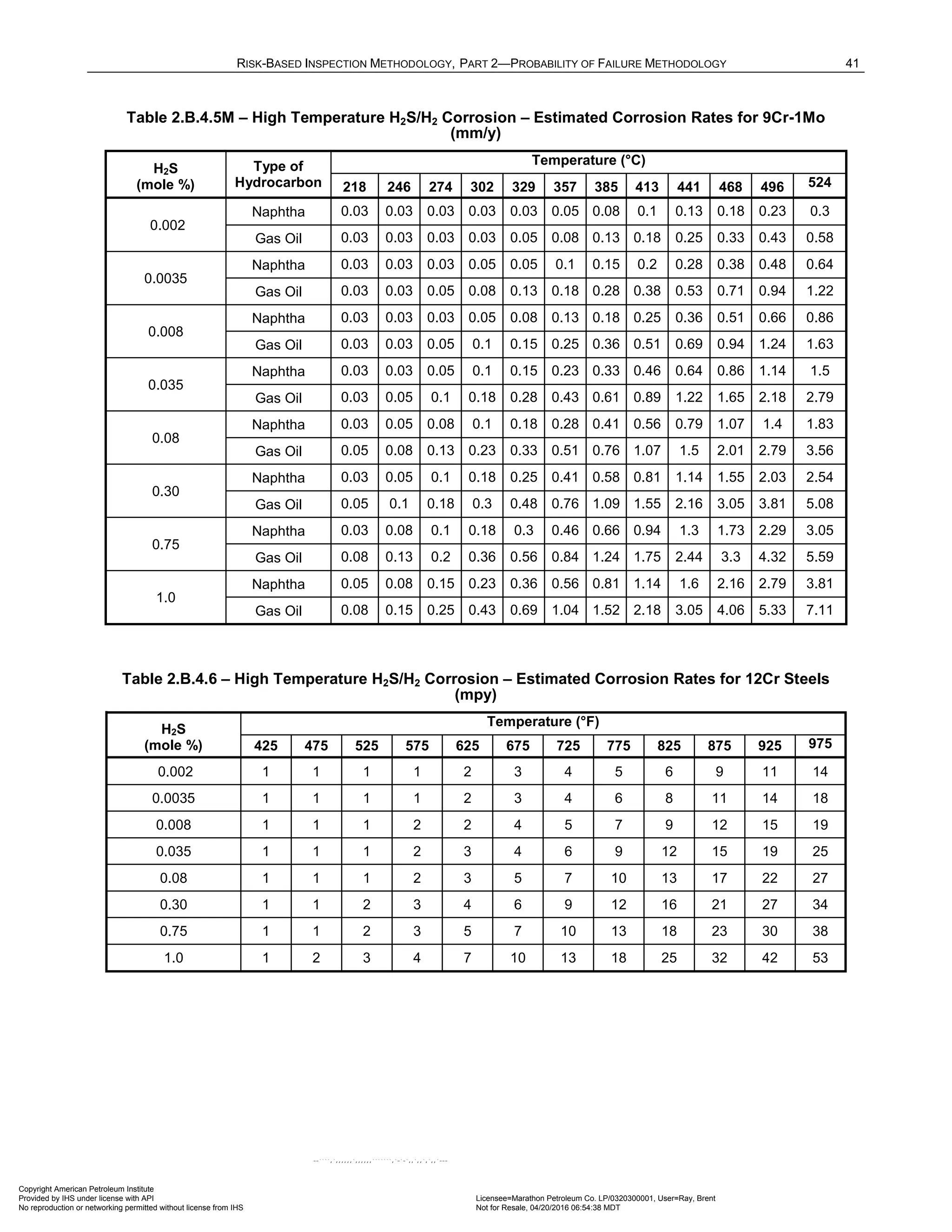
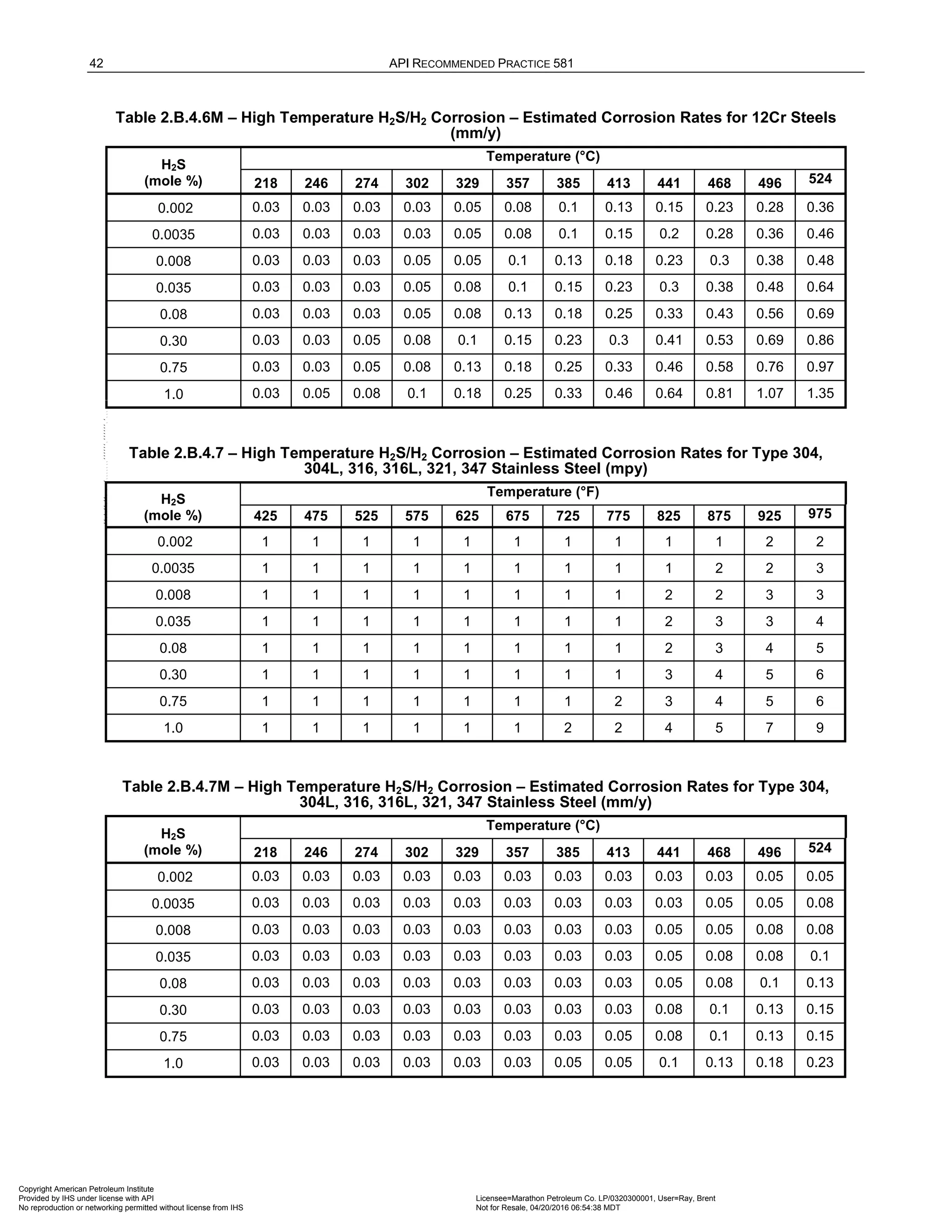
![RISK-BASED INSPECTION METHODOLOGY, PART 2—PROBABILITY OF FAILURE METHODOLOGY 43
2.B.4.6 Figures
Type of Hydrocarbon
(except 12% Cr steel
and 300 Series S.S. )
• Material
• Temperature
• H2S Concentration
Start
Estimated
Corrosion Rate
Determine estimated
corrosion rate from Tables
2.B.4.2 through 2.B.4.7 as
applicable.
Figure 2.B.4.1 – High Temperature H2S/H2 Corrosion – Determination of Corrosion Rate
2.B.5 Sulfuric Acid Corrosion
2.B.5.1 Description of Damage
Sulfuric acid (H2SO4) is one of the most widely used industrial chemicals. One common use of concentrated
H2SO4 is as a catalyst for the alkylation process. H2SO4is a very strong acid that can be extremely corrosive
under certain conditions. The corrosiveness of H2SO4 varies widely, and depends on many factors. Acid
concentration and temperature are the foremost factors that influence corrosion. In addition, velocity effects and
presence of impurities in the acid, especially oxygen or oxidants, can have a significant impact on corrosion.
Although H2SO4corrodes carbon steel, it is the material typically chosen for equipment and piping handling
concentrated H2SO4 at near ambient temperatures. The corrosion rate of steel by H2SO4 as a function of acid
concentration and temperature under stagnant conditions is provided in NACE Publication 5A151 [12]. Stagnant
or low flow (<0.91 m/s or 3 ft/s) conditions typically cause general thinning of carbon steel. The ferrous sulfate
corrosion product film is somewhat protective, and as it builds on the metal surface the corrosion rate
decreases. The mass transfer of ferrous sulfate away from the corroding steel surface is the rate-limiting step for
the corrosion. Acid solution velocity above approximately 0.91 m/s (3 ft/s) (turbulent flow) has a significant
impact on this mass transfer rate and thus the corrosion rate. Corrosion rates for steel pipelines carrying H2SO4
at various conditions and velocities have been calculated from a well-established mathematical model [13]. The
calculated rates were based on pure H2SO4 solutions with no ferrous sulfate present in the acid solution. These
rates for turbulent flow in straight pipes were then multiplied by a factor of 3 (based on experience cited in [13] to
account for the enhanced localized corrosion that occurs at elbows, tees, valves, and areas of internal surface
roughness such as protuberances at welded joints. This provides maximum estimated corrosion rates. Actual
corrosion rates could be 20 to 50% of these estimated maximum corrosion rates.
Although the performance of many alloys in H2SO4service is primarily related to the acid concentration and
temperature, velocity and the presence of an oxidant can play a significant role as well. This is because these
alloys often depend upon formation of a protective oxide film to provide passivity, and therefore corrosion
resistance. The presence of an oxidant usually improves the corrosion performance in H2SO4 service of alloys
such as stainless steel and many nickel alloys. This is not the case with Alloy B-2, which can suffer drastically
high corrosion rates if an oxidant is present in the acid. The corrosion rates provided in these tables are from
published literature, and the corrosion rates for non-aerated acid services are used to provide conservatism,
except for Alloy B-2. This conservatism is appropriate because other acid contaminants and velocity can affect
the material’s passivity. The effect of velocity on corrosion rates is assumed to hold over a wide range of
conditions for very little information on the effect of velocity is published.
Copyright American Petroleum Institute
Provided by IHS under license with API Licensee=Marathon Petroleum Co. LP/0320300001, User=Ray, Brent
Not for Resale, 04/20/2016 06:54:38 MDT
No reproduction or networking permitted without license from IHS
--````,`,,,,,,`,,,,,,```````,`-`-`,,`,,`,`,,`---](https://image.slidesharecdn.com/api581-3rdedition-april2016-240227010601-3bf73ab5/75/Norma-API-581-3rd-Edition-April-2016-pdf-353-2048.jpg)
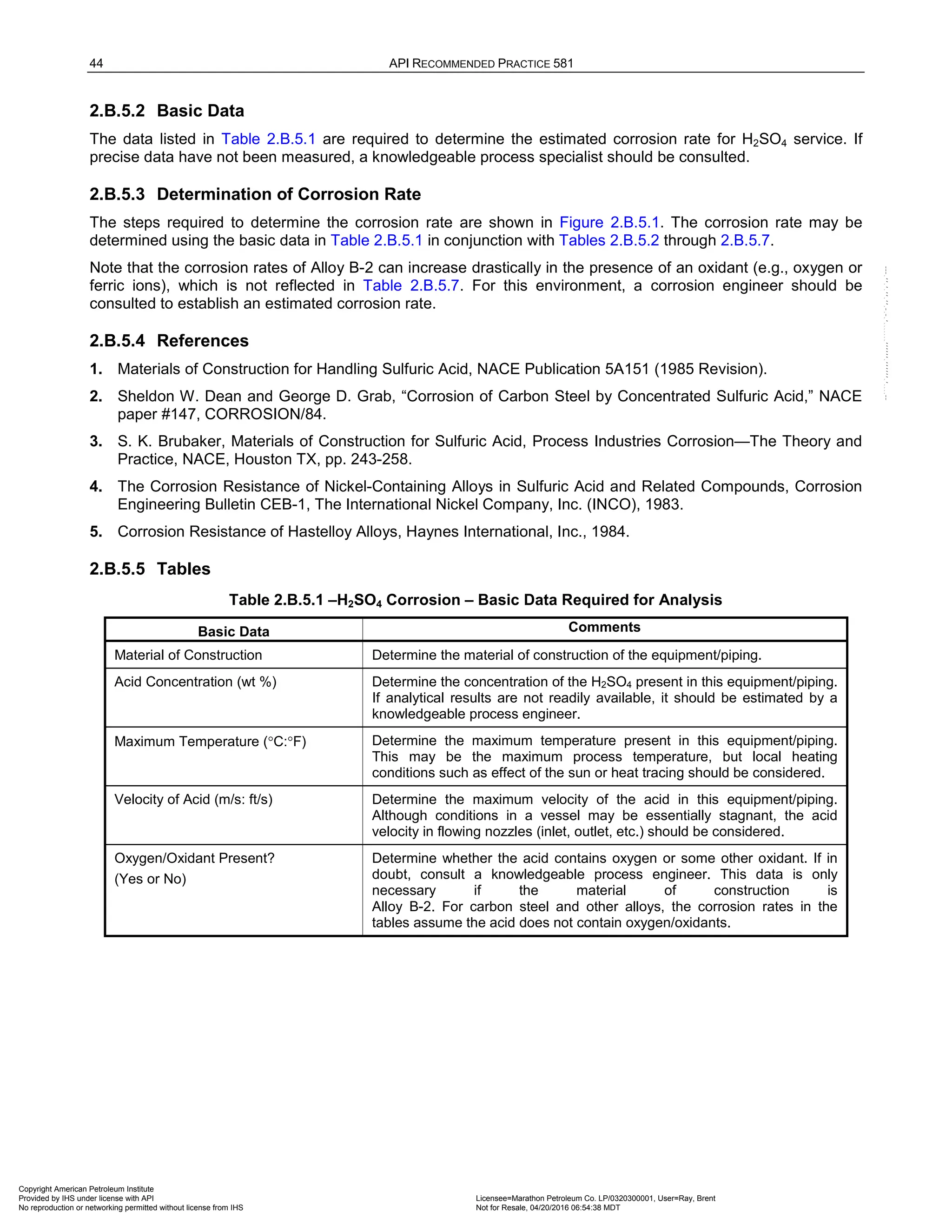
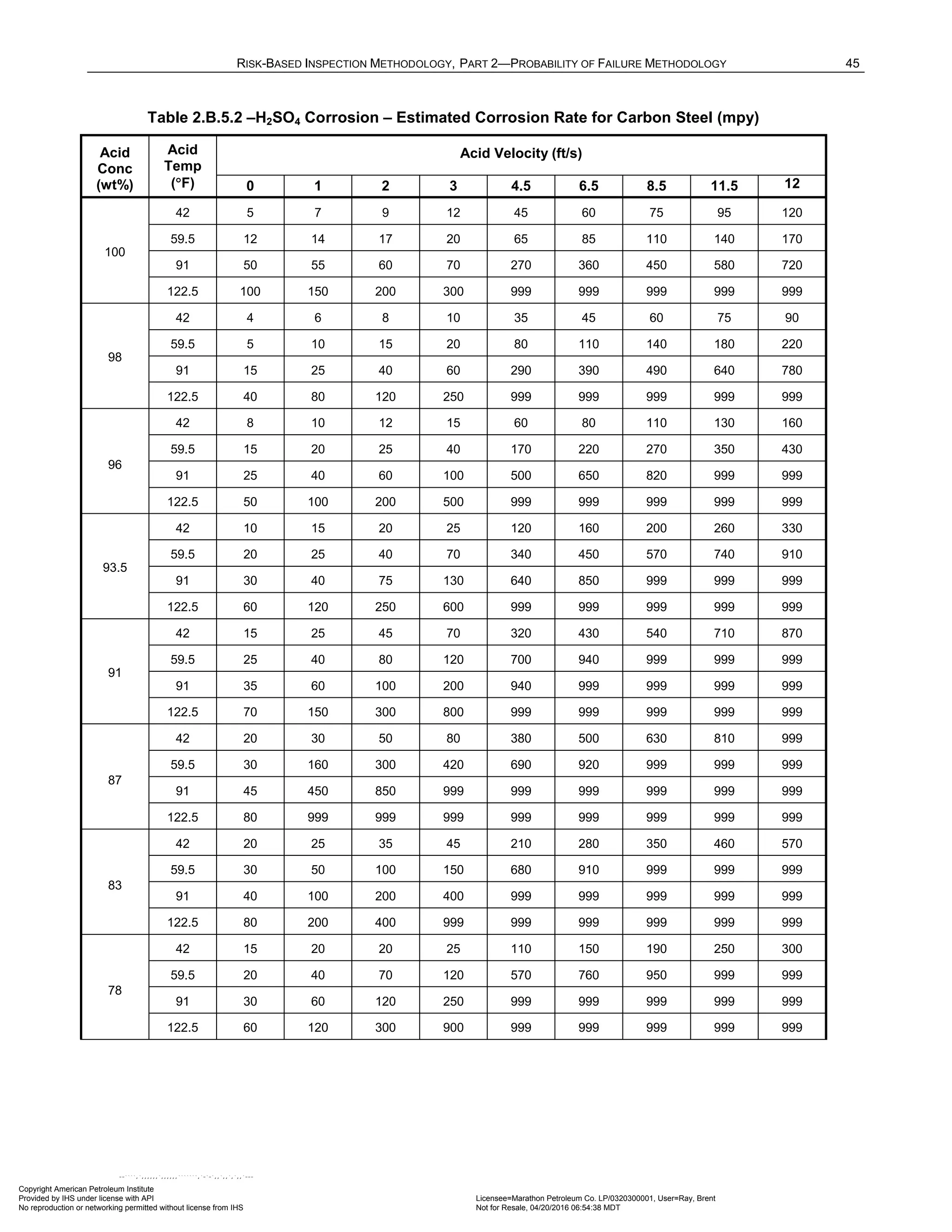
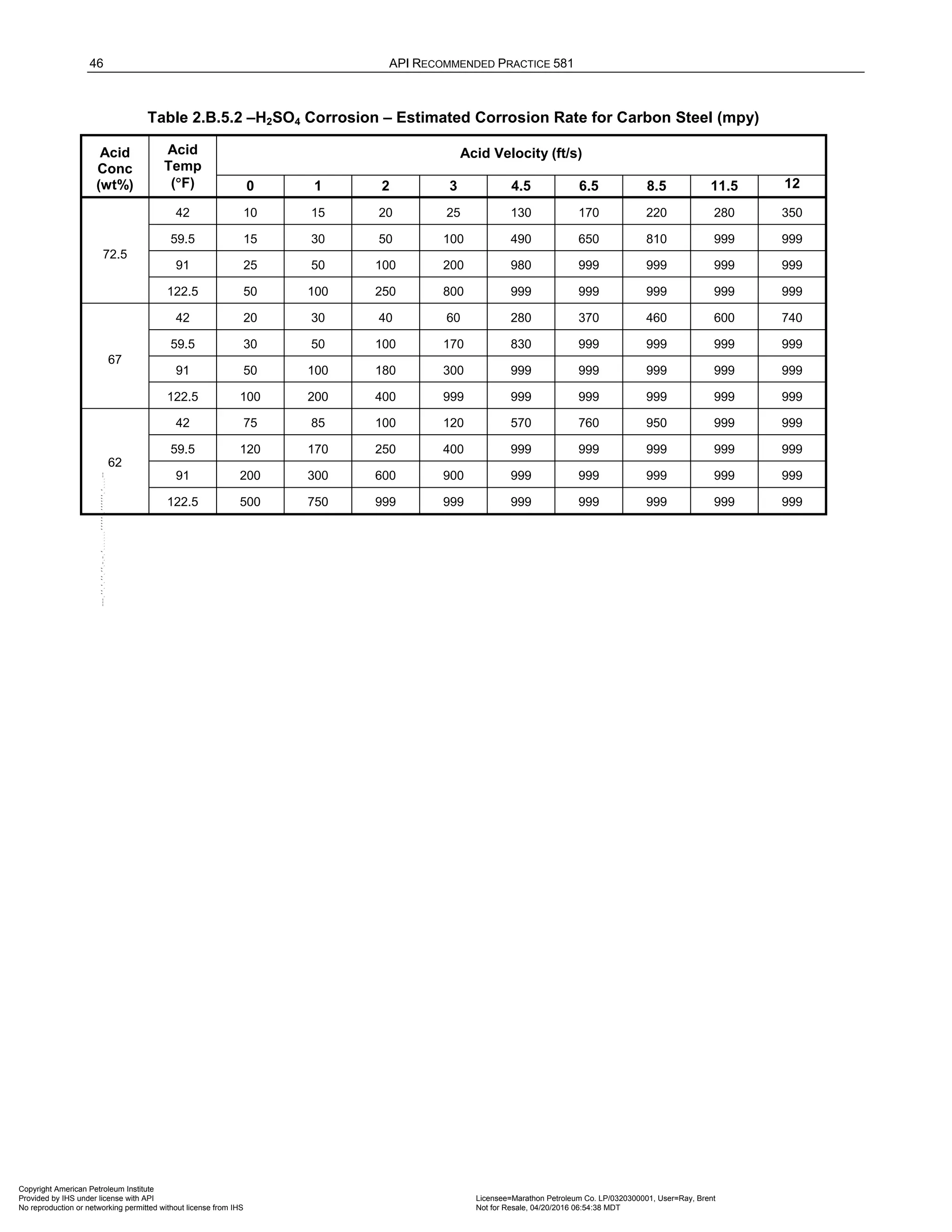
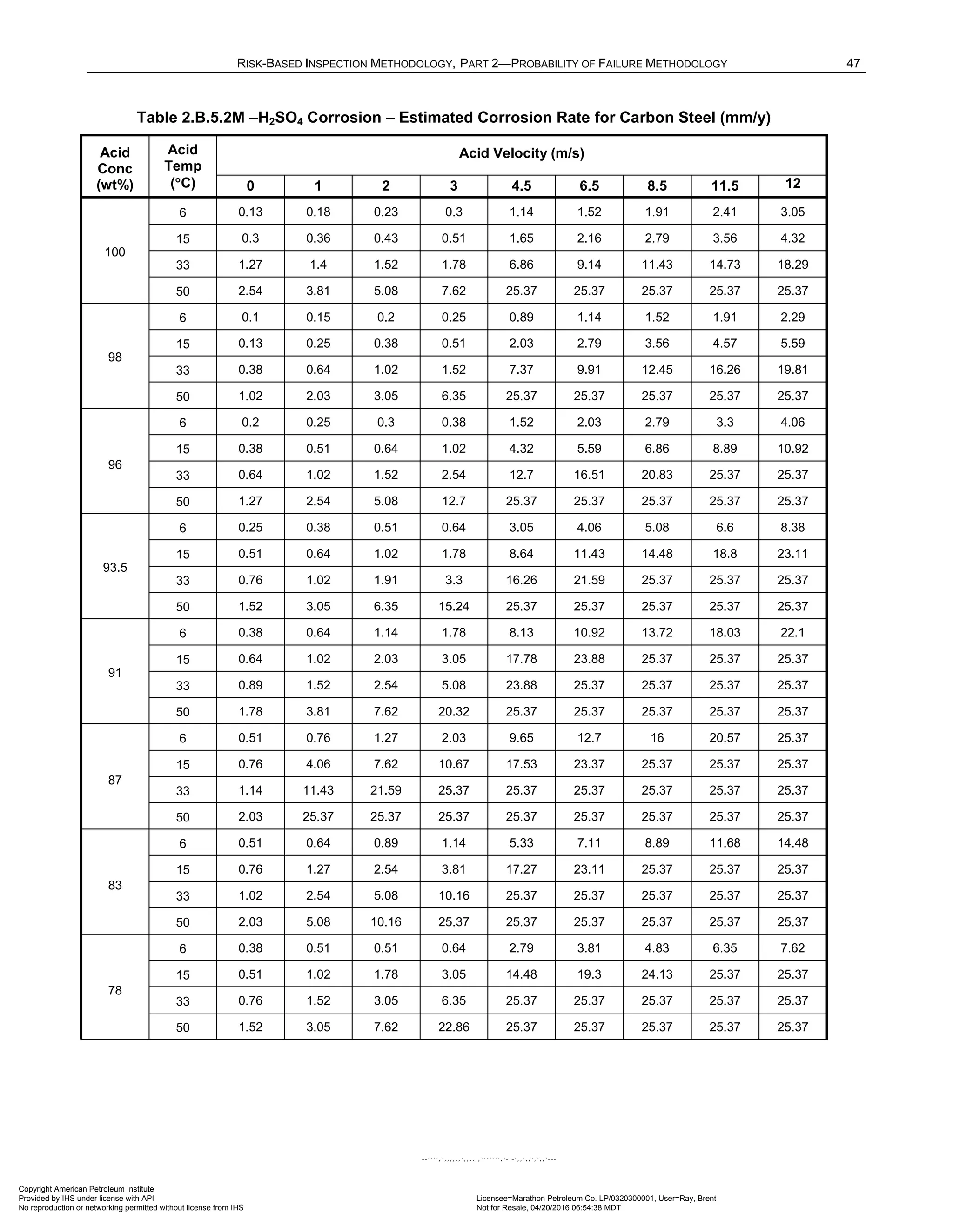
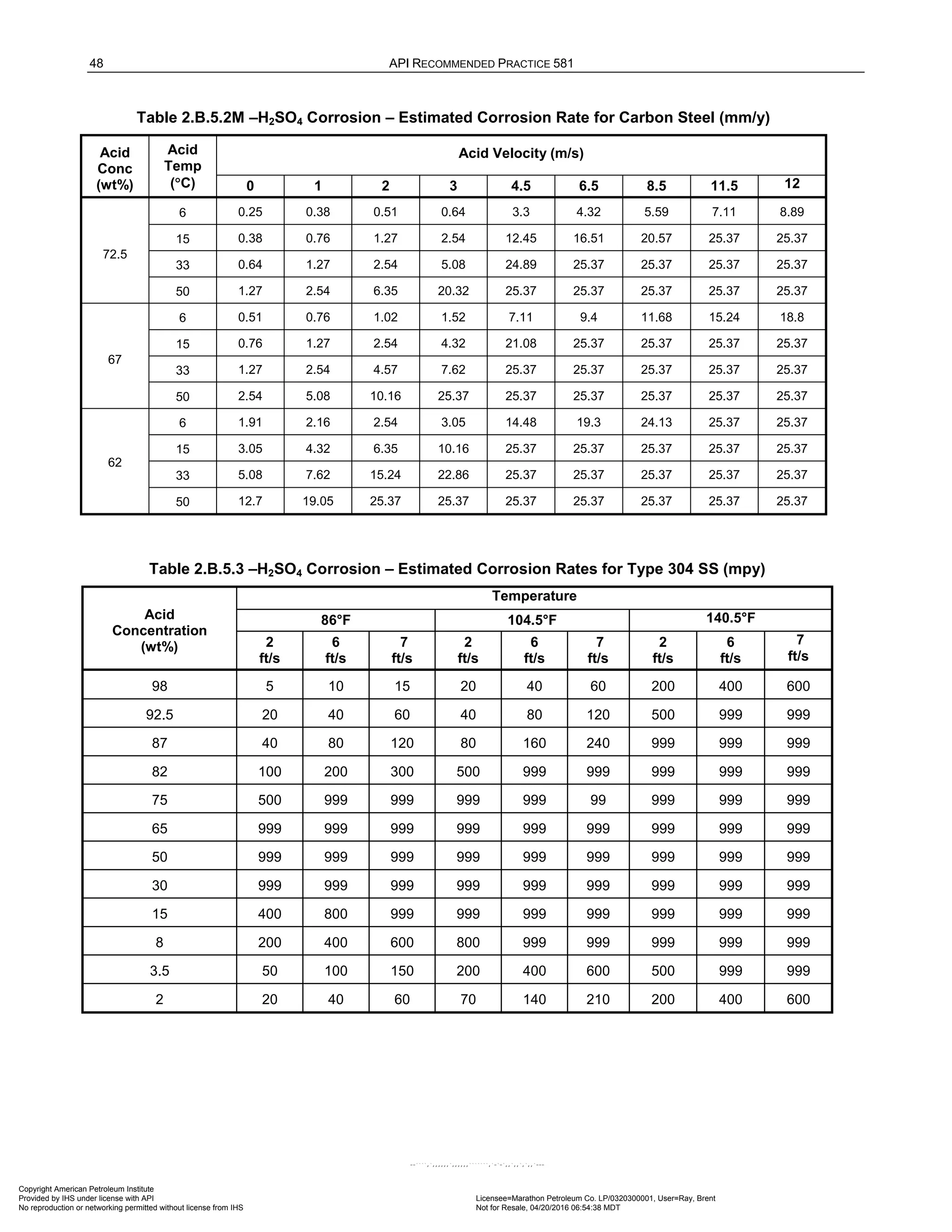
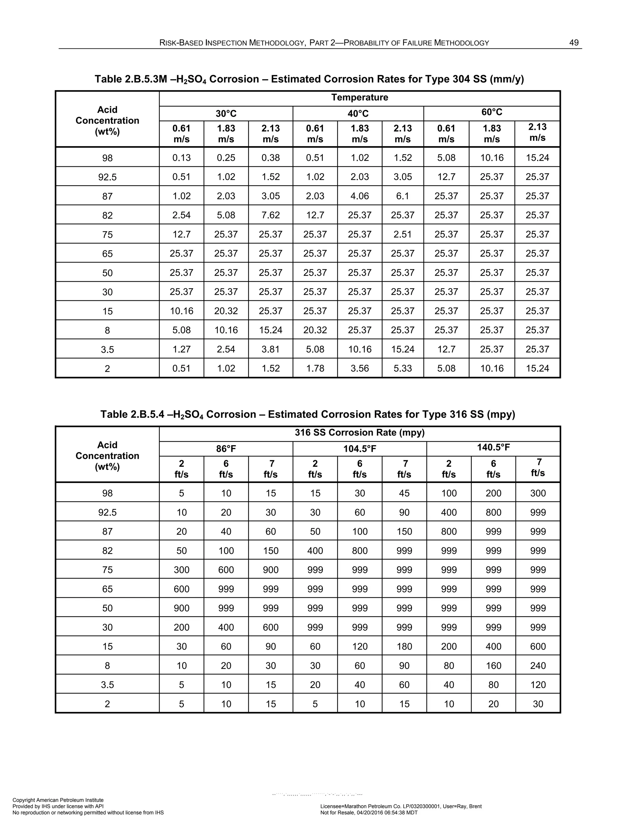
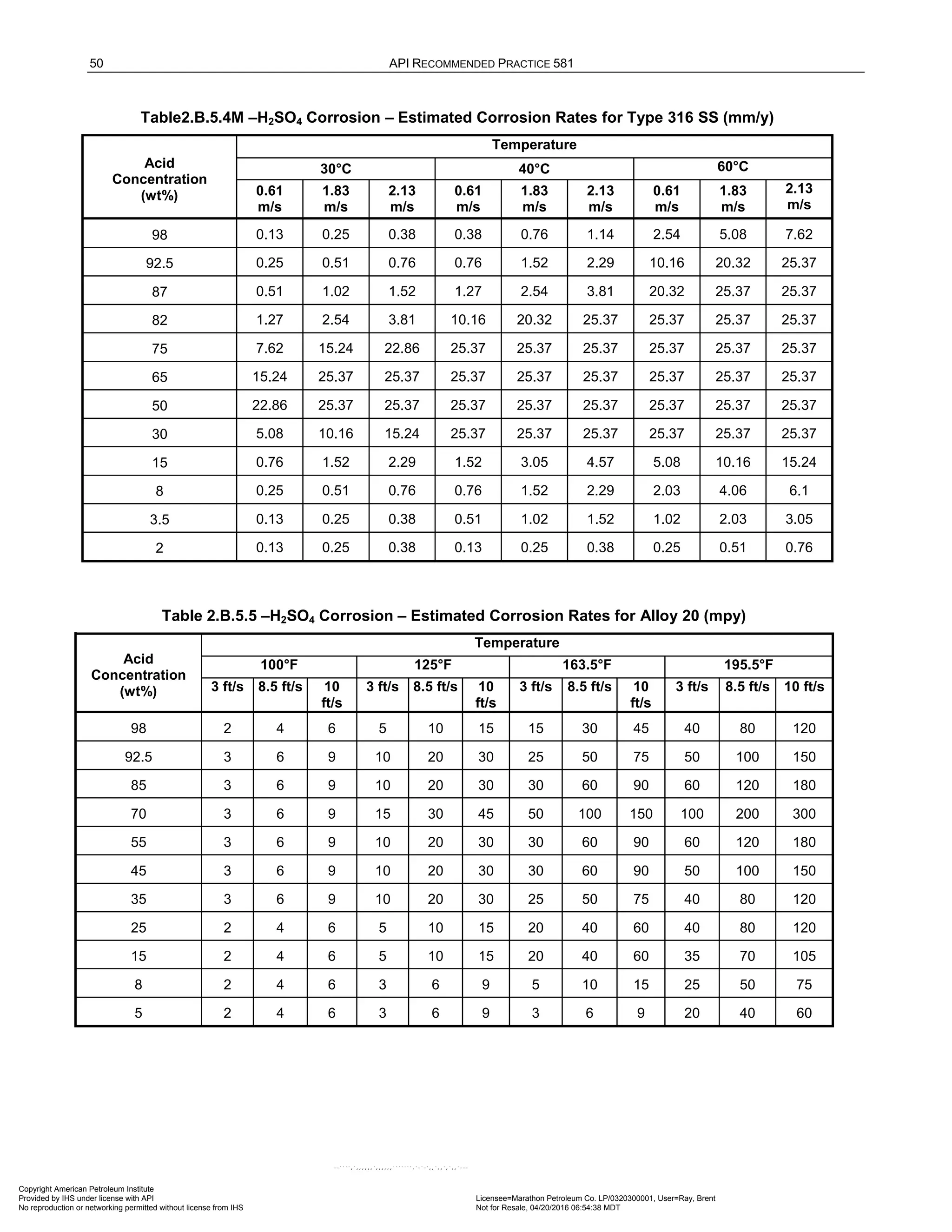
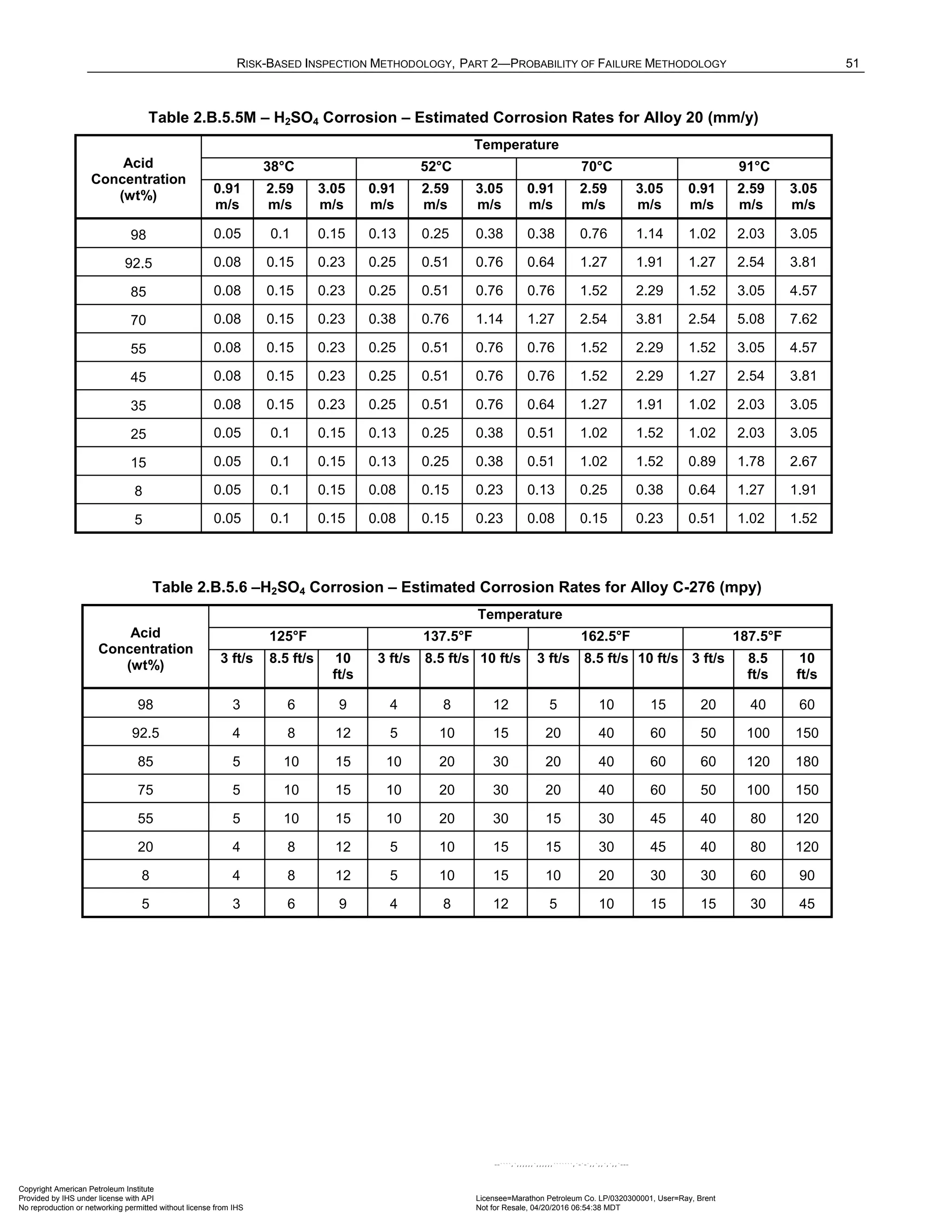
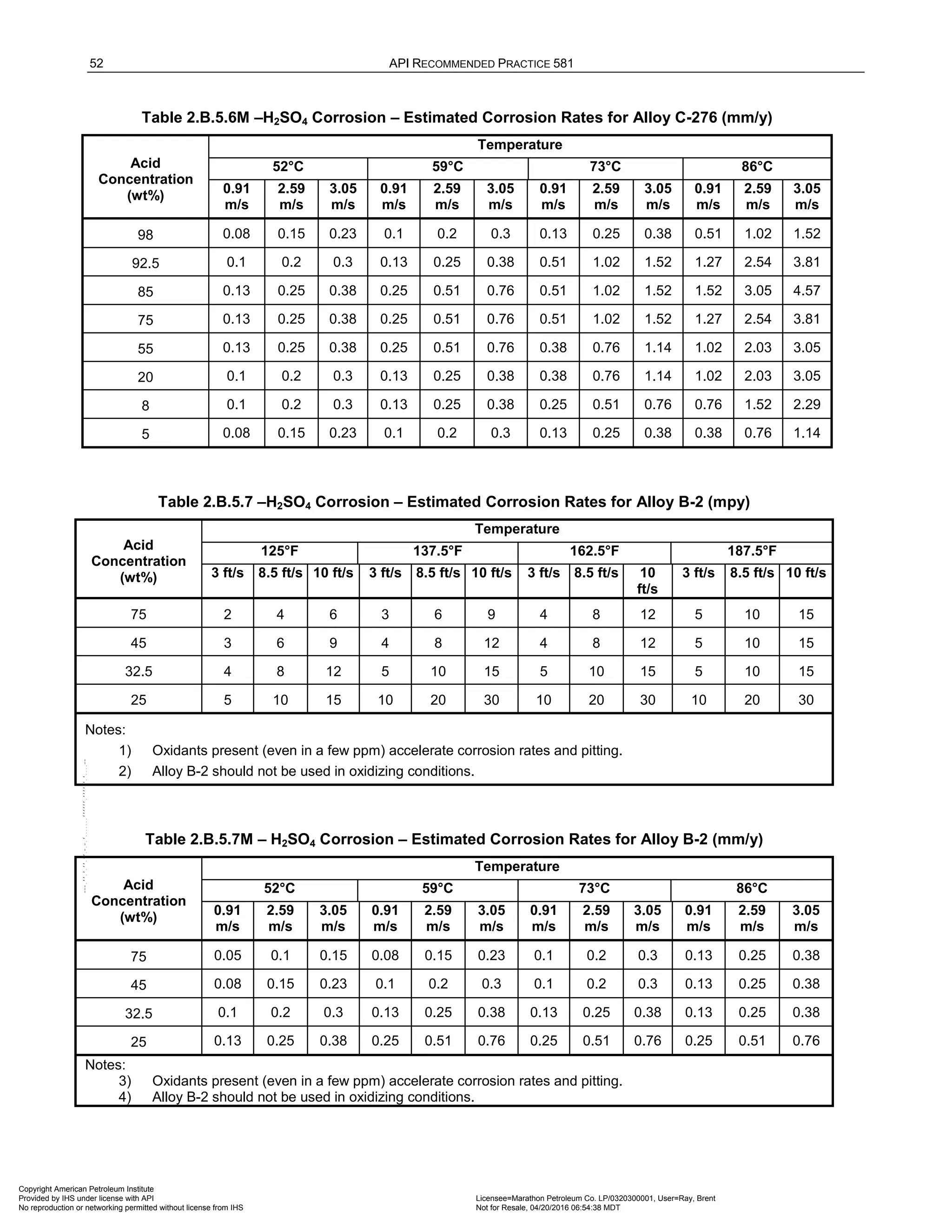
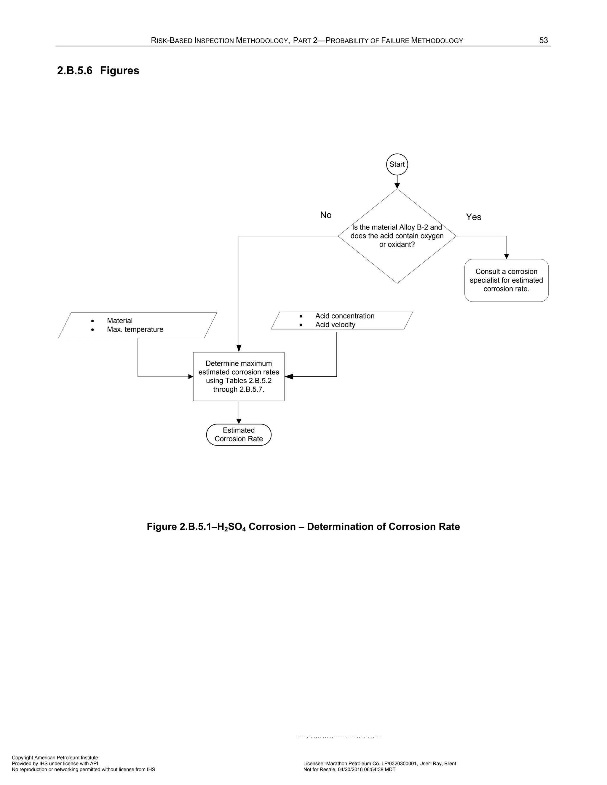
![54 API RECOMMENDED PRACTICE 581
2.B.6 Hydrofluoric Acid Corrosion
2.B.6.1 Description of Damage
Concentrated hydrofluoric acid (HF) is used as the acid catalyst in HF alkylation units. The alkylation reaction
chemically combines an alkane (usually isobutane) with an olefin (butylene, propylene, amylene) in the
presence of the acid catalyst. HF presents severe health hazards as both a liquid and vapor. If spilled, HF may
form a dense, low lying, toxic cloud. Extreme caution should be exercised when using HF.
Corrosion of materials in HF primarily depends on the HF-in-water concentration and the temperature. Other
variables, such as velocity, turbulence, aeration, impurities, etc., can strongly influence corrosion. Some metals
will form a protective fluoride film or scale which protects the surface. Loss of this protective film, especially
through high velocity or turbulence, will likely result in greatly accelerated corrosion rates. Corrosion in 80% and
stronger HF-in-water solutions is equivalent to corrosion in anhydrous hydrofluoric acid (AHF, 200 ppm H2O).
Below 80% HF, the acid is considered aqueous and metal corrosion is highly temperature and velocity
dependent and usually accelerated. The usual HF-in-water concentrations in typical HF alkylation units are
96%–99+% and the temperatures are generally below 66°C (150°F). Under these conditions carbon steel is
widely used for all equipment except where close tolerances are required for operation (i.e., pumps, valves,
instruments). Where close tolerances are required and at temperatures over 66°C (150°F) to approximately
149°C (300°F), Alloy 400 is typically used.
Accelerated corrosion from water dilution of the acid is often encountered in low points (bleeders, line pockets,
etc.) if unit dry out leaves residual free water in these areas.
2.B.6.2 Basic Data
The data listed in Table 2.B.6.1 are required to determine the estimated corrosion rate for sulfuric acid service. If
precise data have not been measured, a knowledgeable process specialist should be consulted.
2.B.6.3 Determination of Corrosion Rate
The steps required to determine the corrosion rate are shown in Figure 2.B.6.1. The corrosion rate may be
determined using the basic data in Table 2.B.6.1 in conjunction with Tables 2.B.6.2 through 2.B.6.3.
It is important to note that the corrosion rate is very high in the initial stages of exposure to HF as the protective
fluoride scale is being established. Once established, the fluoride scale protects the steel resulting in low
corrosion rates unless the scale is disturbed or removed.
Alloy steels have been found to exhibit higher corrosion rates than mild carbon steel in both dilute and
concentrated HF and generally are not specified for this service. Higher alloys are sometimes used in HF
service and corrosion rates, if unknown, should be obtained from published literature or from the manufacturer
[20]. It is important to consider the galvanic effects of welding carbon steel to Alloy 400 or other corrosion
resistant alloys. Accelerated and localized attack of the carbon steel may result from galvanic coupling.
Increased rates of corrosion have also been reported in carbon steels which contain high levels of residual
elements, notably Cu, Ni, and Cr [22].
Corrosion caused by HF results in general thinning except in the event of potential galvanic attack. The
presence of HF may also result in hydrogen stress cracking and blistering. These degradation modes are
considered in Part 2, paragraph 14.1.
Copyright American Petroleum Institute
Provided by IHS under license with API Licensee=Marathon Petroleum Co. LP/0320300001, User=Ray, Brent
Not for Resale, 04/20/2016 06:54:38 MDT
No reproduction or networking permitted without license from IHS
--````,`,,,,,,`,,,,,,```````,`-`-`,,`,,`,`,,`---](https://image.slidesharecdn.com/api581-3rdedition-april2016-240227010601-3bf73ab5/75/Norma-API-581-3rd-Edition-April-2016-pdf-364-2048.jpg)
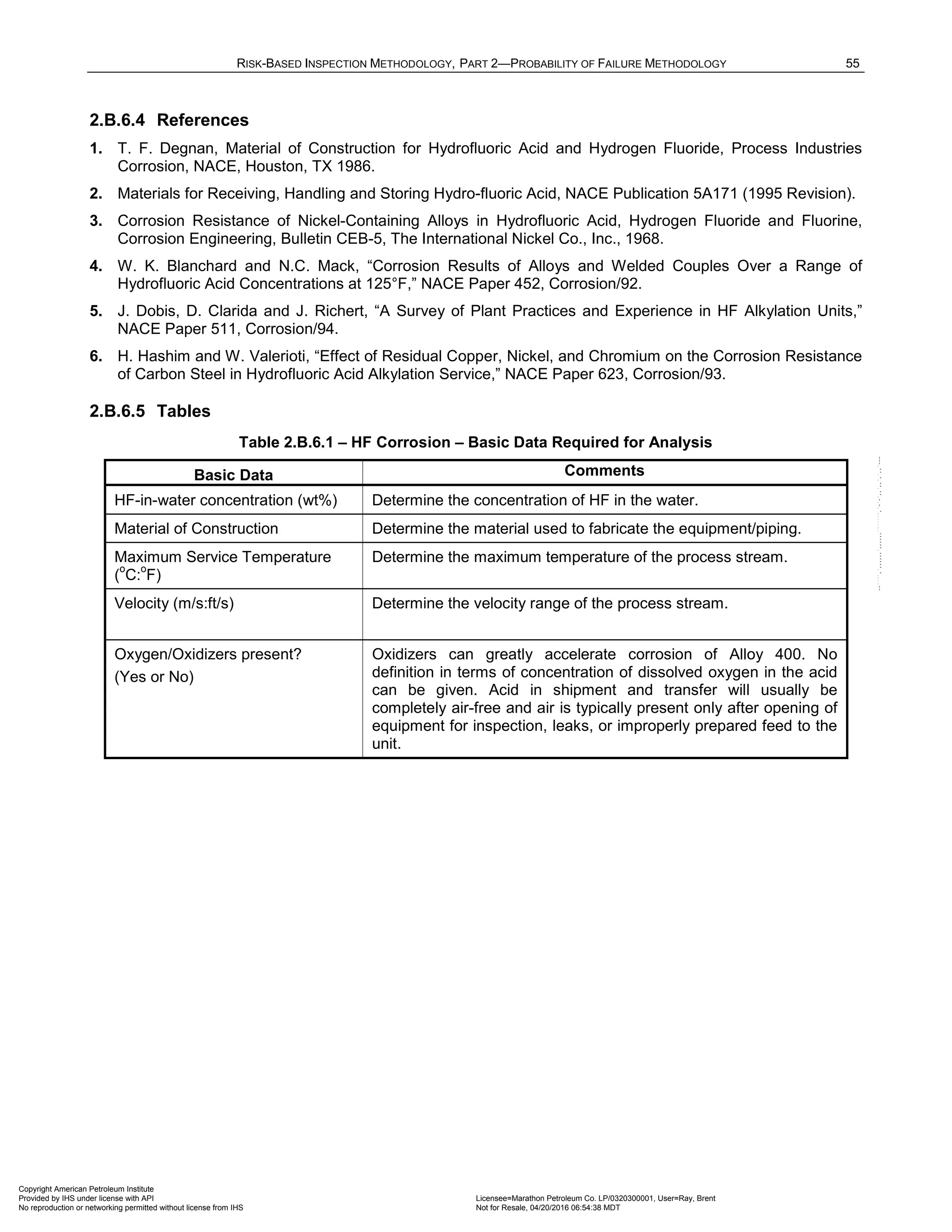
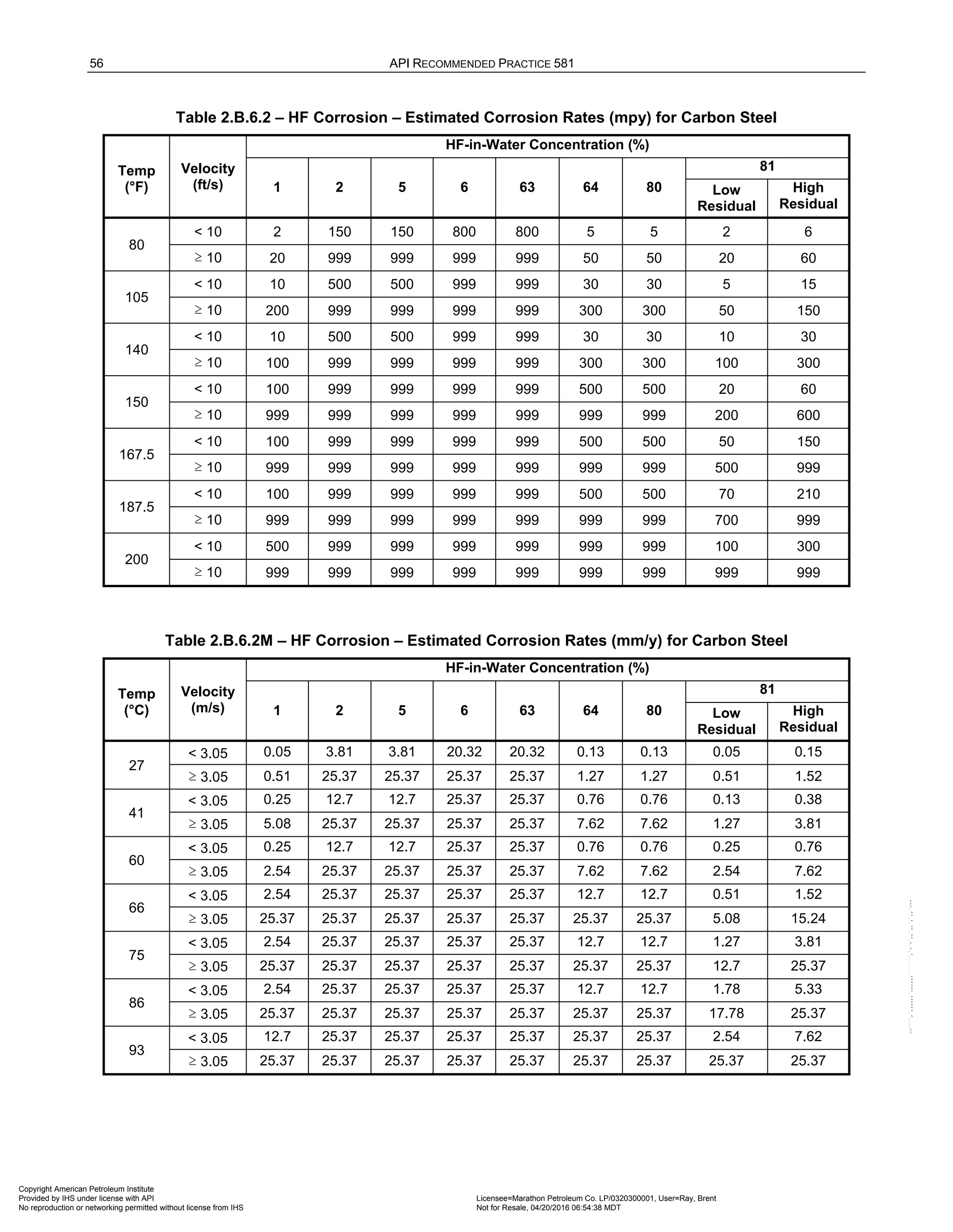
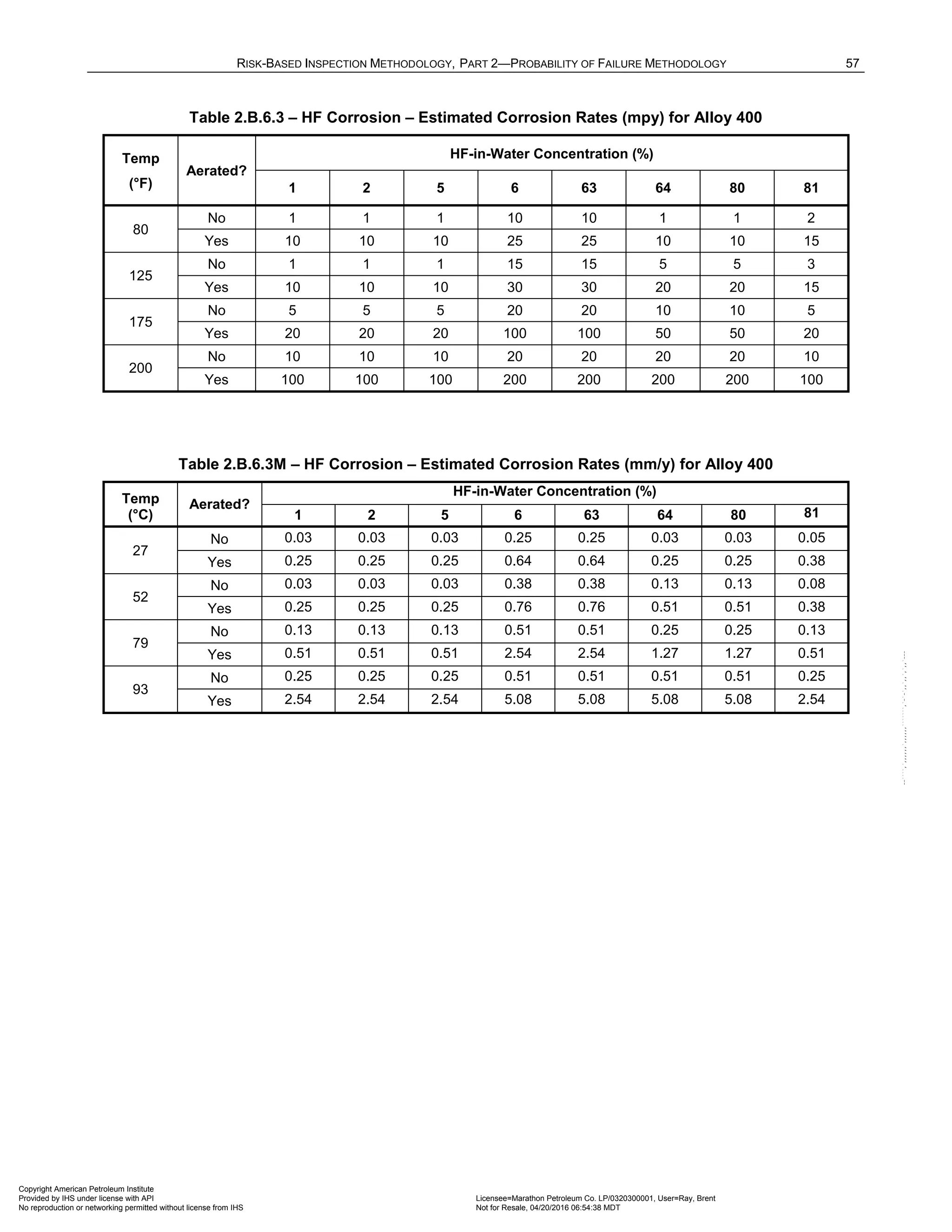
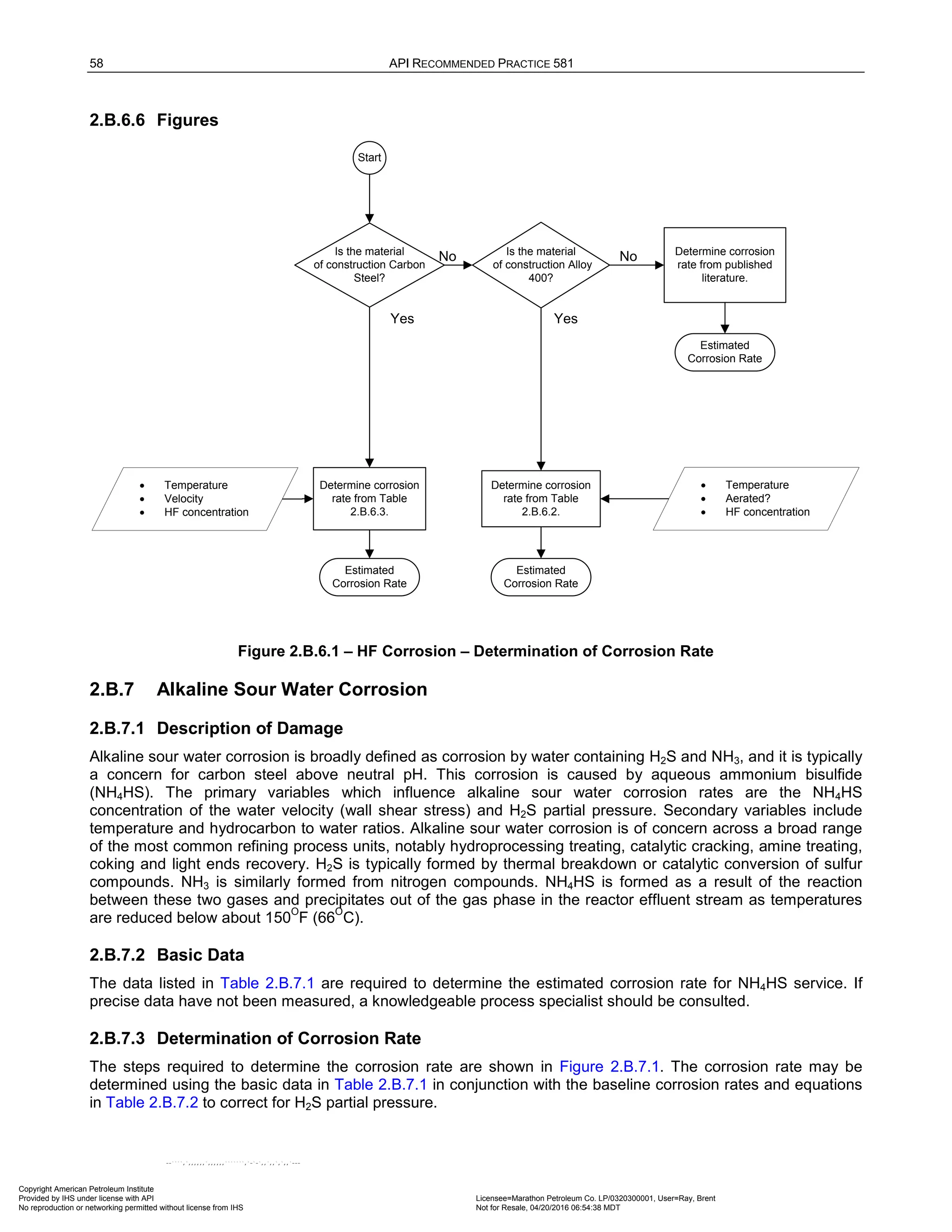
![RISK-BASED INSPECTION METHODOLOGY, PART 2—PROBABILITY OF FAILURE METHODOLOGY 59
2.B.7.4 References
1.
1. R. L. Piehl, “Survey of Corrosion in Hydrocracker Effluent Air Coolers,” Materials Protection, January, 1976
2. E. F. Ehmke, “Corrosion Correlation with Ammonia and Hydrogen Sulfide in Air Coolers,” Materials Protection, July,
1975.
3. D. G. Damin and J. D. McCoy, “Prevention of Corrosion in Hydrodesulfurizer Air Coolers and Condensers,” Materials
Performance, December, 1978, pp. 23–26 (See also NACE Corrosion/78 paper #131).
4. C. Scherrer, M. Durrieu, and G. Jarno, “Distillate and Resid Hydroprocessing: Coping with High Concentrations of
Ammonium Bisulfide in the Process Water,” Materials Performance, November, 1980, pp 25–31 (See also NACE
CORROSION/79 paper #27).
5. R.J. Horvath, M.S. Cayard and R.D. Kane, "Prediction and Assessment of Ammonium Bisulfide Corrosion Under
Refinery Sour Water Service Conditions,” CORROSION/06, paper no. 06576 (Houston, TX: NACE, 2006).
2.B.7.5 Tables
Table 2.B.7.1 – Alkaline Sour Water Corrosion – Basic Data Required for Analysis
Basic Data Comments
NH4HS concentration (wt%) Determine the NH4HS concentration of the condensed water. It is suggested to determine
this value with ionic process models. However, approximate values may be calculated from
analyses of H2S and NH3 as follows:
• If wt% H2S < 2 x (wt% NH3), wt% NH4HS =1.5 x (wt% H2S)
• If wt% H2S > 2 x (wt% NH3), wt% NH4HS =3.0 x (wt% H2S)
Stream Velocity, m/s [ft/s] The vapor phase velocity should be used in a two-phase system. The liquid phase velocity
should be used in a liquid full system.
H2S partial pressure, psia
[kPa]
Determine the partial pressure of H2S by multiplying the mole% of H2S in the gas phase by
the total system pressure.
Table 2.B.7.2 – Alkaline Sour Water Corrosion – Baseline Corrosion Rates for Carbon
Steel (mpy)
NH4HS
(wt%)
Velocity (ft/s)
10 15 20 25 30
2 3 4 5 8 11
5 6 9 12 15 18
10 20 27 35 43 50
15 45 70 100 150 200
Note:
1. For pH2S<50 psia, 2
max ( 50) ,0
25
Baseline CR
Adjusted CR pH S Baseline CR
= ⋅ − + ⋅
2. For pH2S>50 psia, 2
max ( 50) ,0
40
Baseline CR
Adjusted CR pH S Baseline CR
= ⋅ − +
Copyright American Petroleum Institute
Provided by IHS under license with API Licensee=Marathon Petroleum Co. LP/0320300001, User=Ray, Brent
Not for Resale, 04/20/2016 06:54:38 MDT
No reproduction or networking permitted without license from IHS
--````,`,,,,,,`,,,,,,```````,`-`-`,,`,,`,`,,`---](https://image.slidesharecdn.com/api581-3rdedition-april2016-240227010601-3bf73ab5/75/Norma-API-581-3rd-Edition-April-2016-pdf-369-2048.jpg)
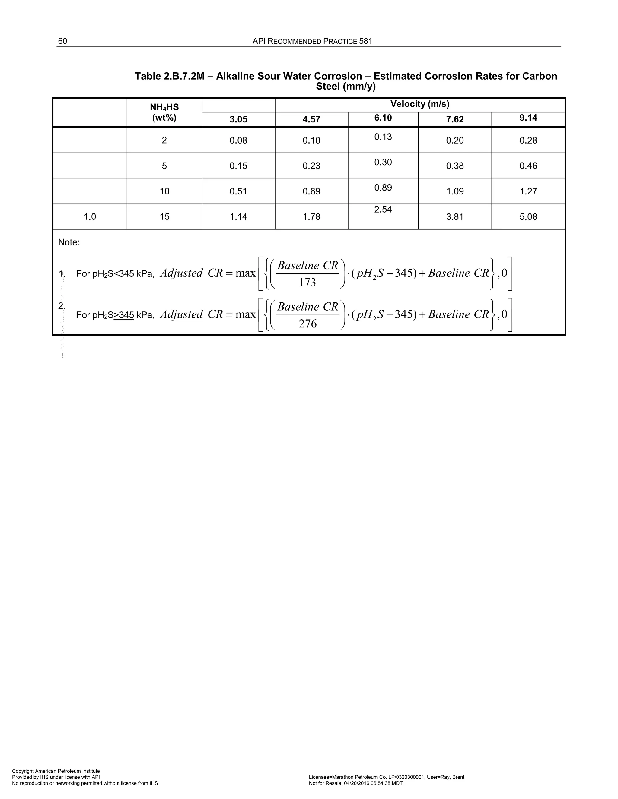
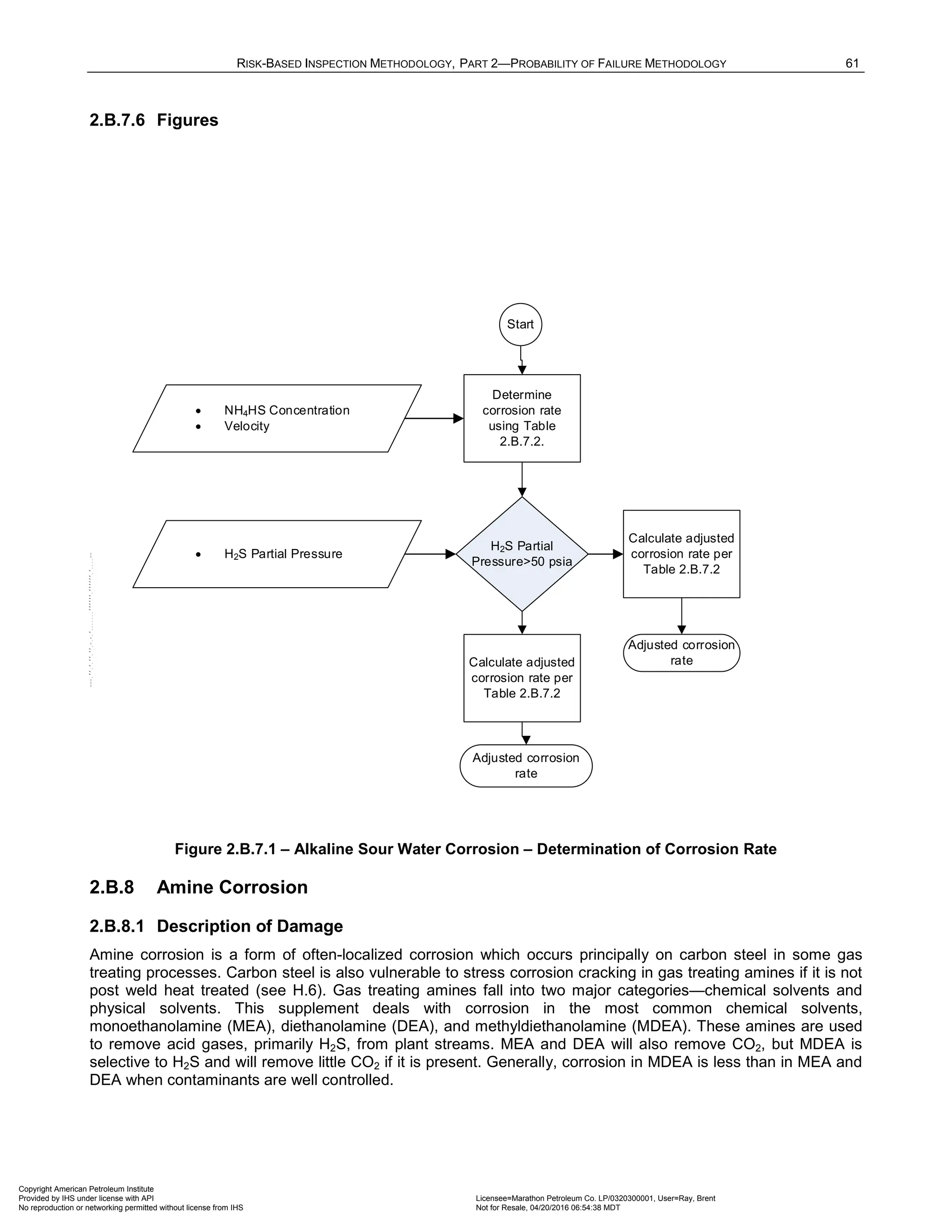
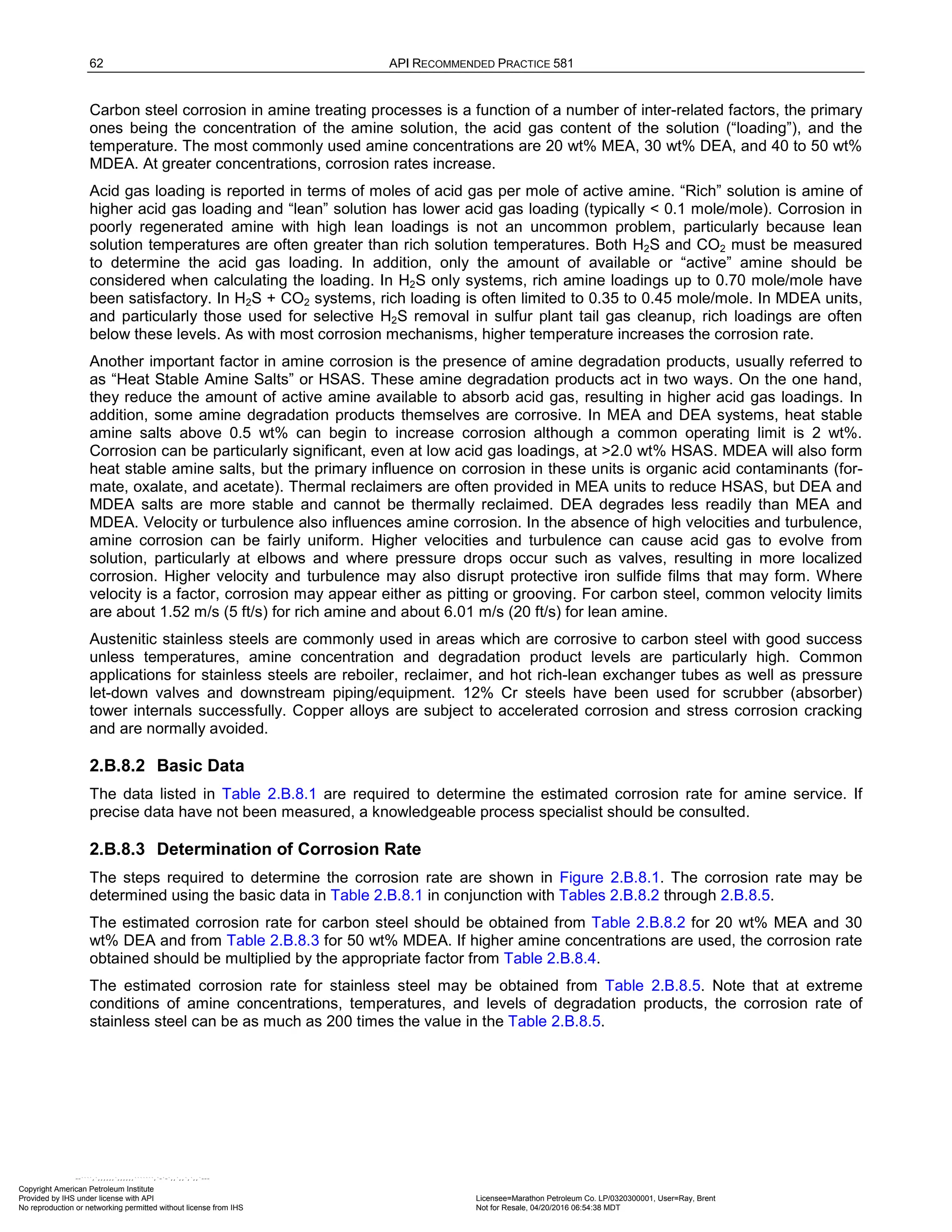
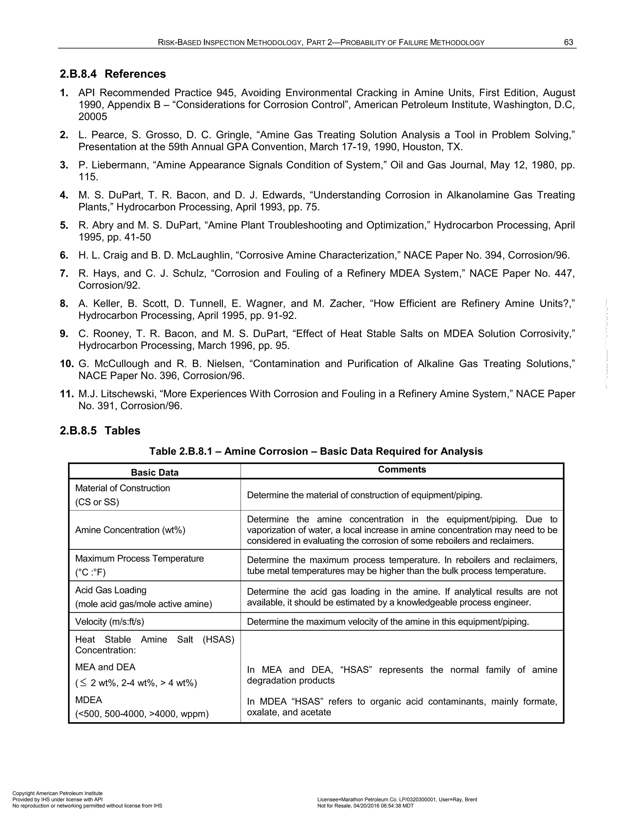
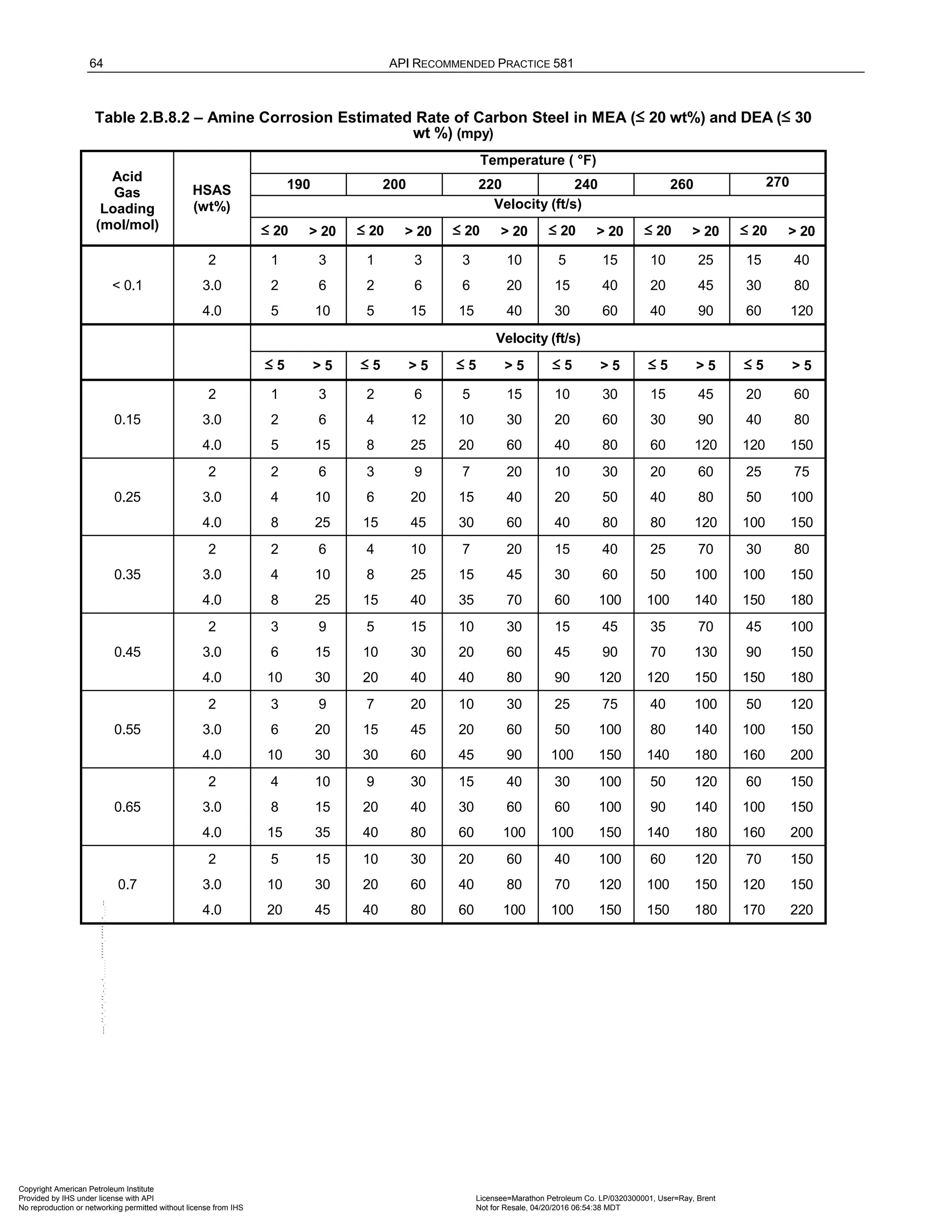
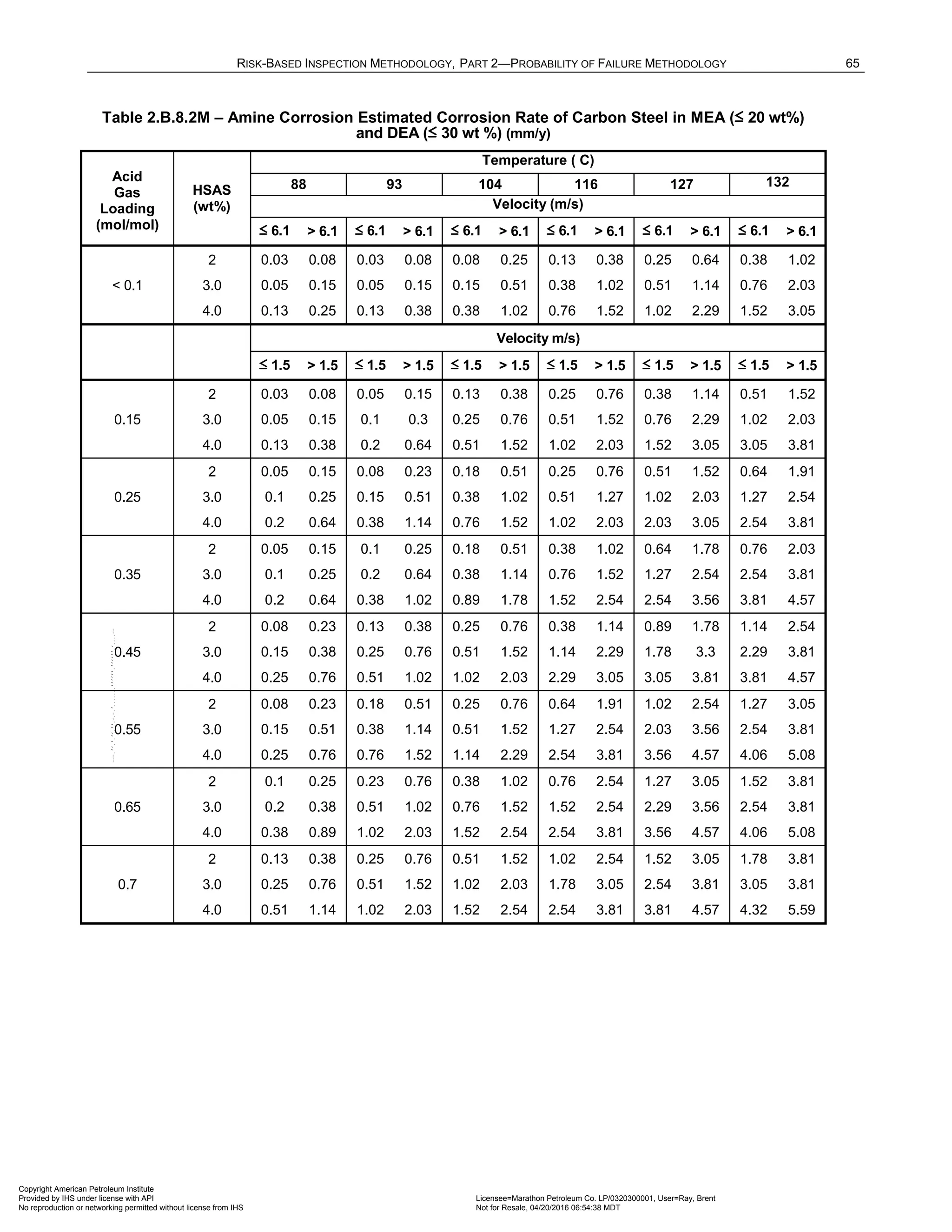

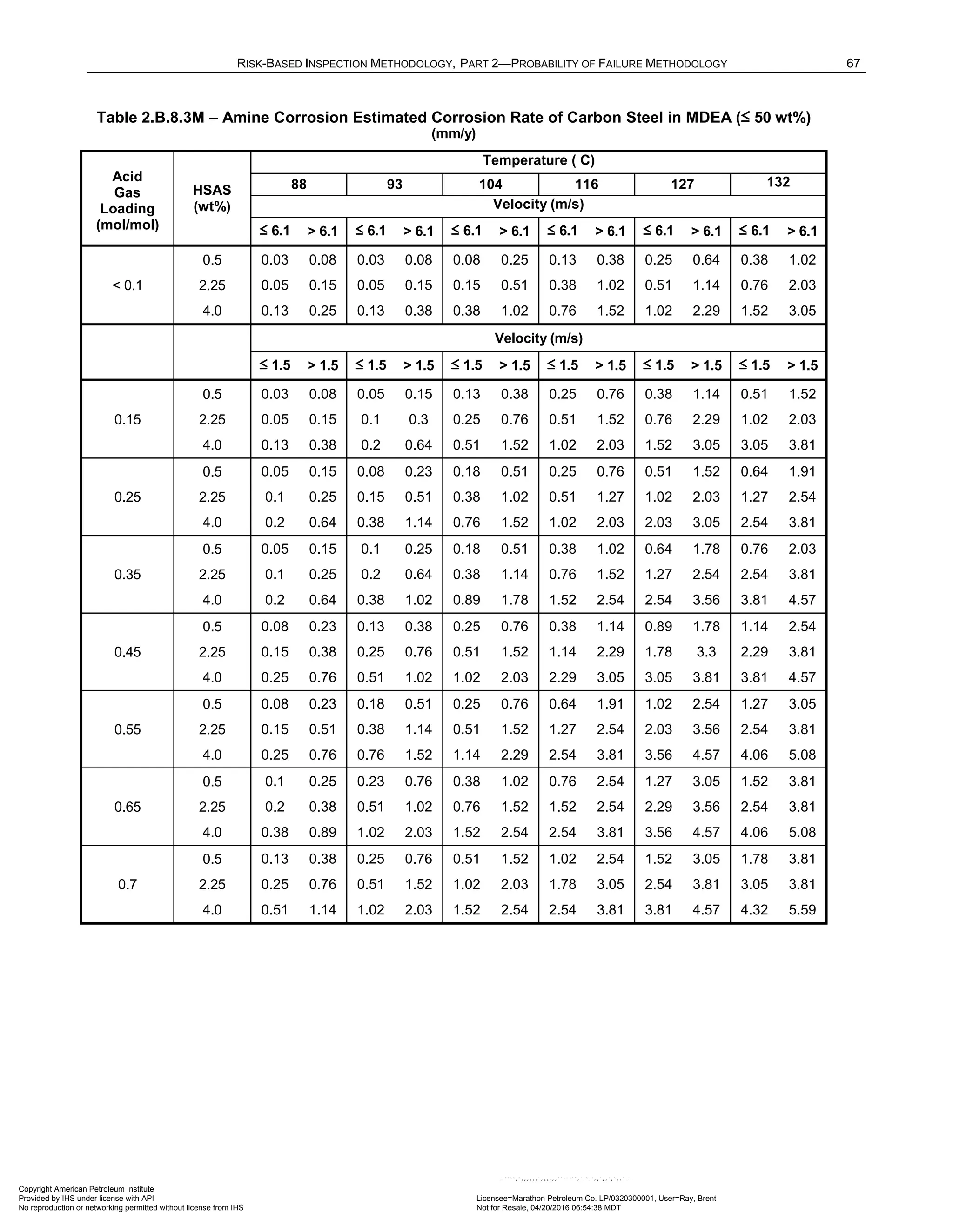
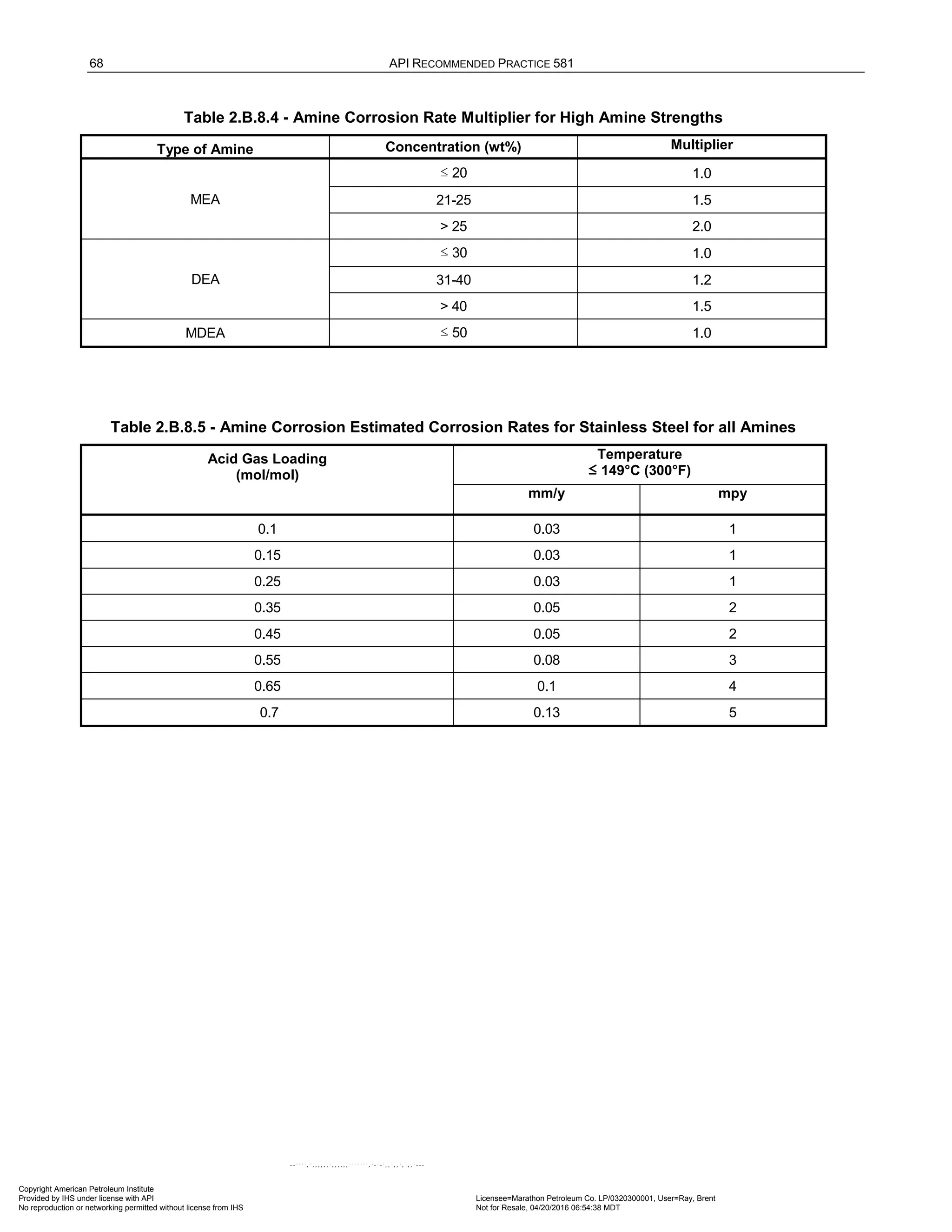
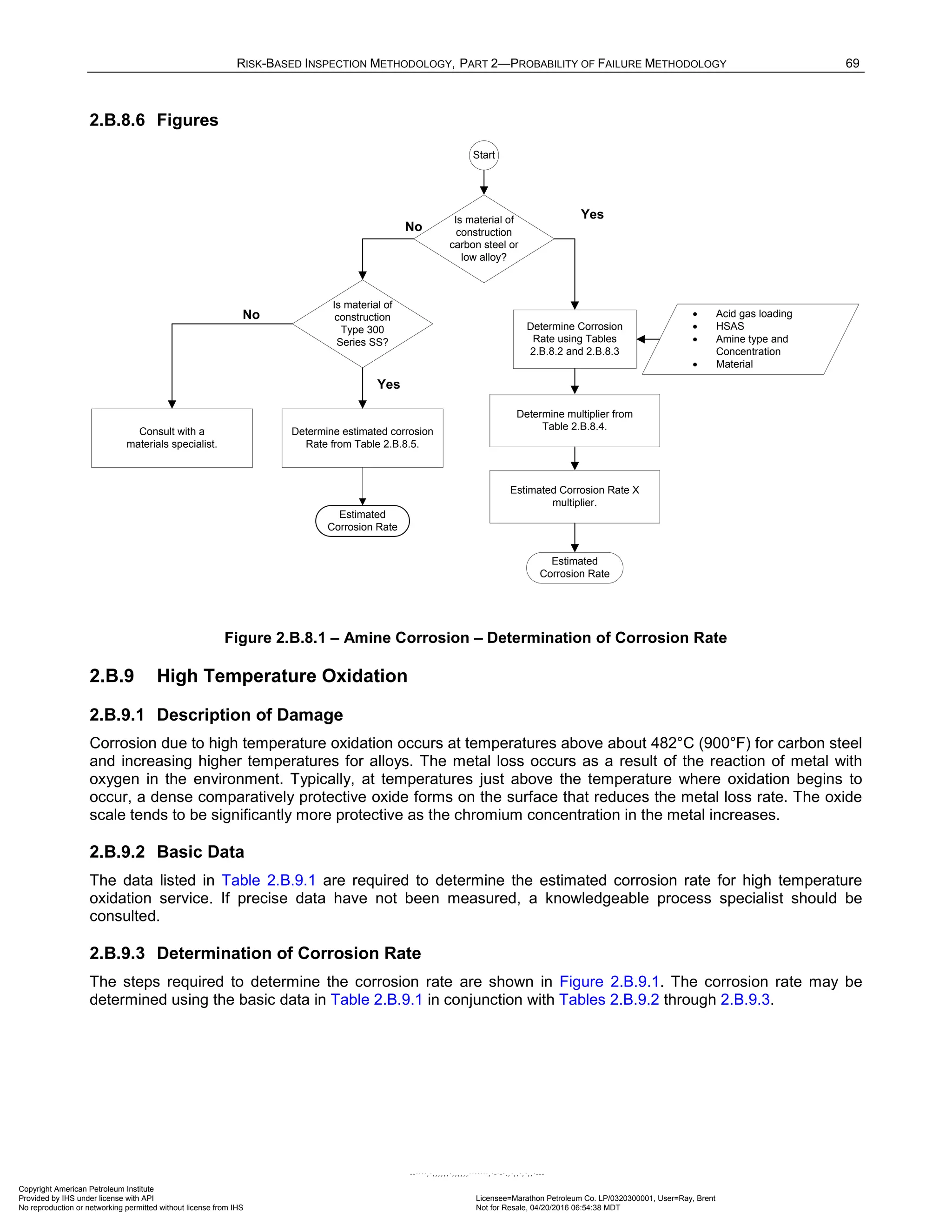
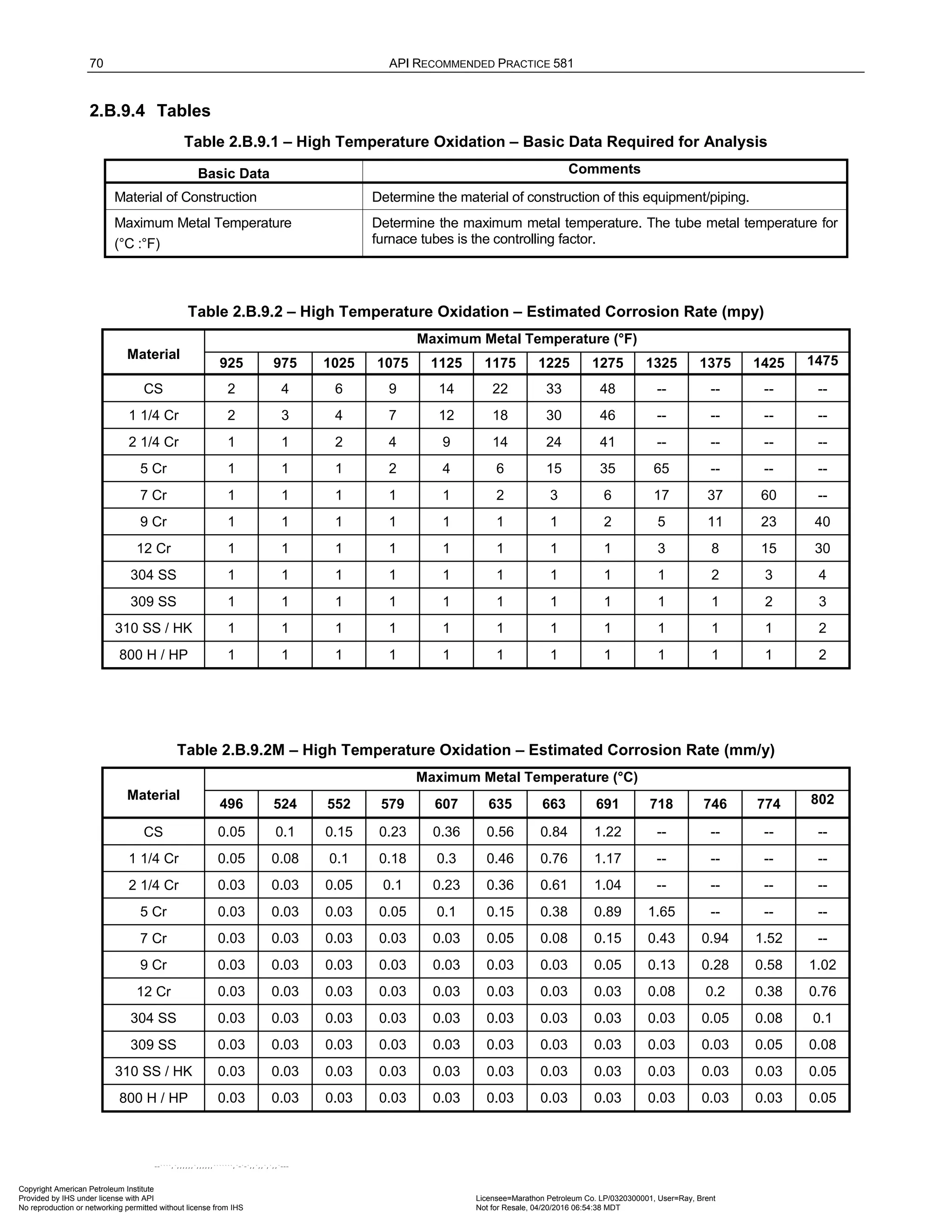
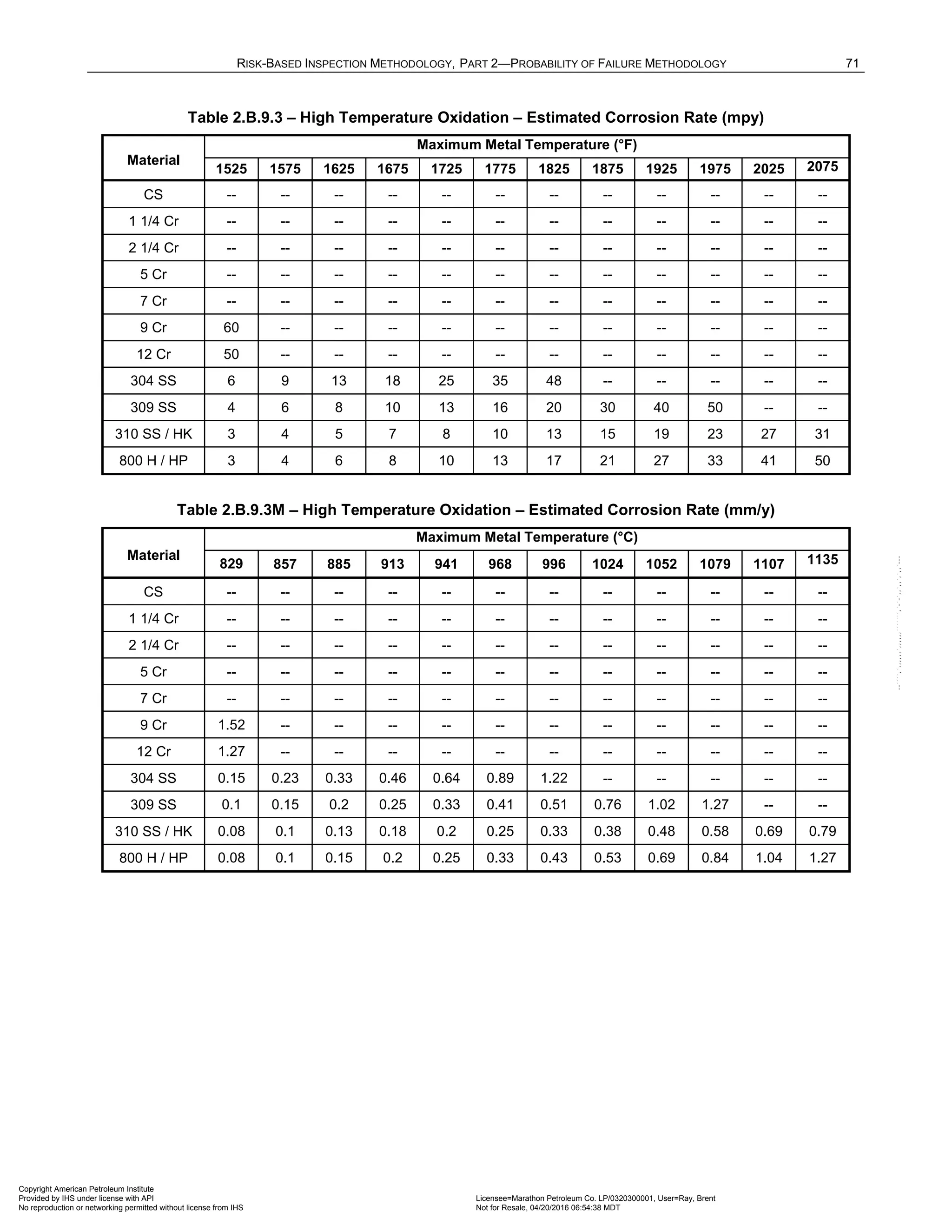
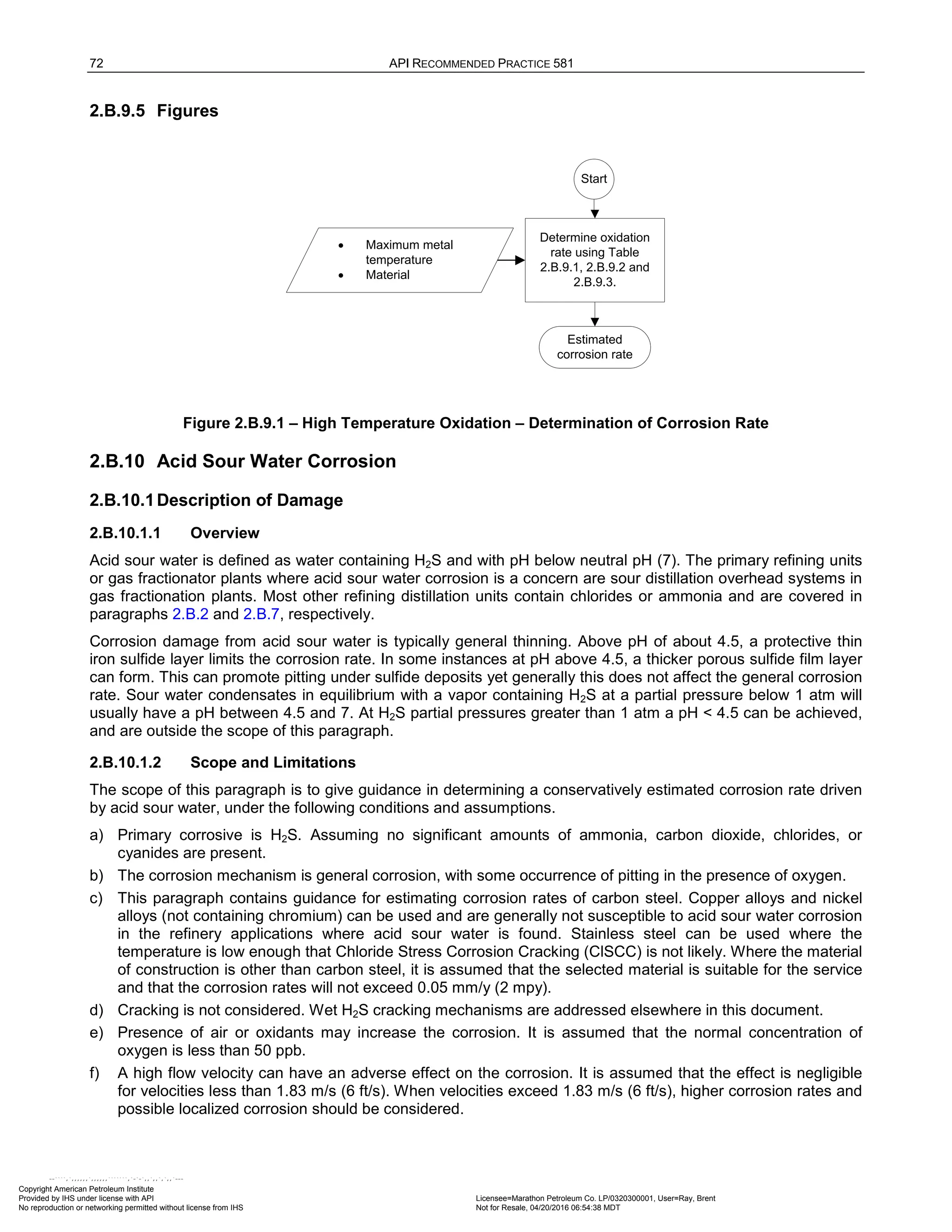
![RISK-BASED INSPECTION METHODOLOGY, PART 2—PROBABILITY OF FAILURE METHODOLOGY 73
The base corrosion rate is estimated from the pH level and temperature. An adjustment is made for oxygen
content. Other factors, such as content of chlorides, cyanides, etc. are relevant, but are considered less
significant for the end result in this context. The result is a conservative value for the estimated corrosion rate.
2.B.10.2Basic Data
The data listed in Table 2.B.10.1 is required to estimate the rate of corrosion rate in acid sour water. If precise
data have not been measured, a knowledgeable process specialist should be consulted.
2.B.10.3Determination of Corrosion Rate
The steps required to determine the corrosion rate are shown in Figure 2.B.10.1. If the pH is less than 4.5, then
the corrosion rate shall be calculated using paragraph 2.B.2. If the pH is greater than 7, then the corrosion rate
is calculated using paragraph 2.B.7. Otherwise, the corrosion rate of carbon steel exposed to acid sour water is
computed using Equation (2.B.1).
= ⋅ ⋅
ph O V
CR CR F F (2.B.1)
The base corrosion rate, pH
C , of carbon steel exposed to acid sour water as a function of pH is provided in
Table 2.B.10.2. The corrosion rate can vary significantly with level of dissolved oxygen. The modification factor
for the corrosion rate as a function of the oxygen content factor, O
F , is provided in Table 2.B.10.3. The
corrosion rate also varies with fluid velocity. The modification factor for fluid velocity is given by the following
equations.
For SI units, use Equations (2.B.2) through (2.B.4),
1.0
V
F = when velocity < 1.83 m/s (2.B.2)
0.82 0.5
V
F velocity
= ⋅ − when 1.83 m/s < velocity < 6.10 m/s (2.B.3)
5.0
V
F = when velocity > 6.10 m/s (2.B.4)
For US Customary units, use Equations (2.B.5) through (2.B.7),
1.0
V
F = when velocity < 6 ft/s (2.B.5)
0.25 0.5
V
F velocity
= ⋅ − when 6 ft/s < velocity < 20 ft/s (2.B.6)
5.0
V
F = when velocity > 20 ft/s (2.B.7)
2.B.10.4Nomenclature
CR is the corrosion rate
ph
CR is the base corrosion rate as a function of pH
O
F is the corrosion rate correction for oxygen
V
F is the corrosion rate correction for velocity
velocity is the fluid velocity, m/s [ft/s]
2.B.10.5References
1. Joerg Gutzeit, ”Corrosion of Steel by Sulfides and Cyanides in Refinery Condensate Water”, Materials
Protection, December 1968, p. 17-23.
2. R.H. Hausler and N.D. Coble, “Corrosion Control in Crude Unit Overhead Systems”, paper 42-72 at API
37th Midyear Meeting, May 10, 1972.
Copyright American Petroleum Institute
Provided by IHS under license with API Licensee=Marathon Petroleum Co. LP/0320300001, User=Ray, Brent
Not for Resale, 04/20/2016 06:54:38 MDT
No reproduction or networking permitted without license from IHS
--````,`,,,,,,`,,,,,,```````,`-`-`,,`,,`,`,,`---](https://image.slidesharecdn.com/api581-3rdedition-april2016-240227010601-3bf73ab5/75/Norma-API-581-3rd-Edition-April-2016-pdf-383-2048.jpg)
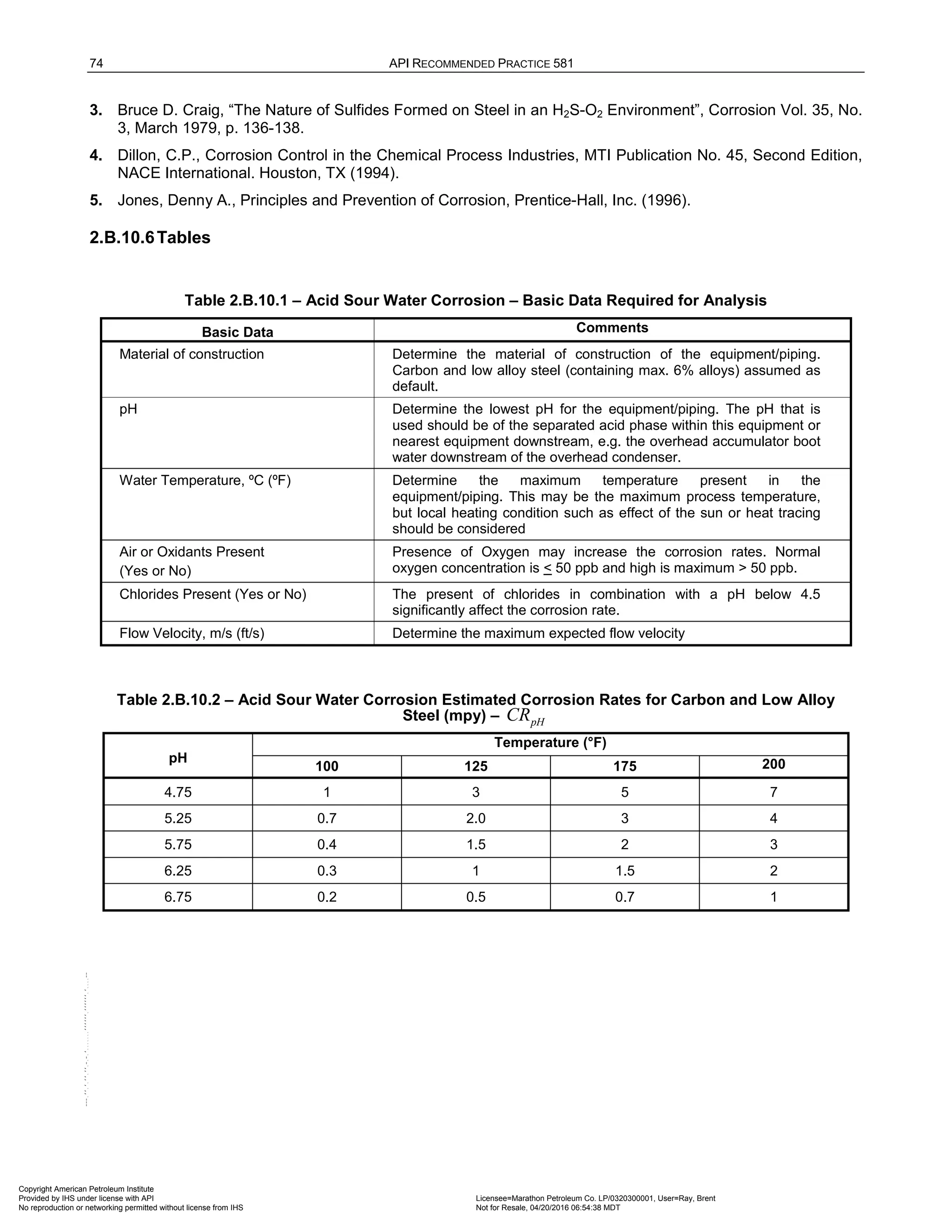
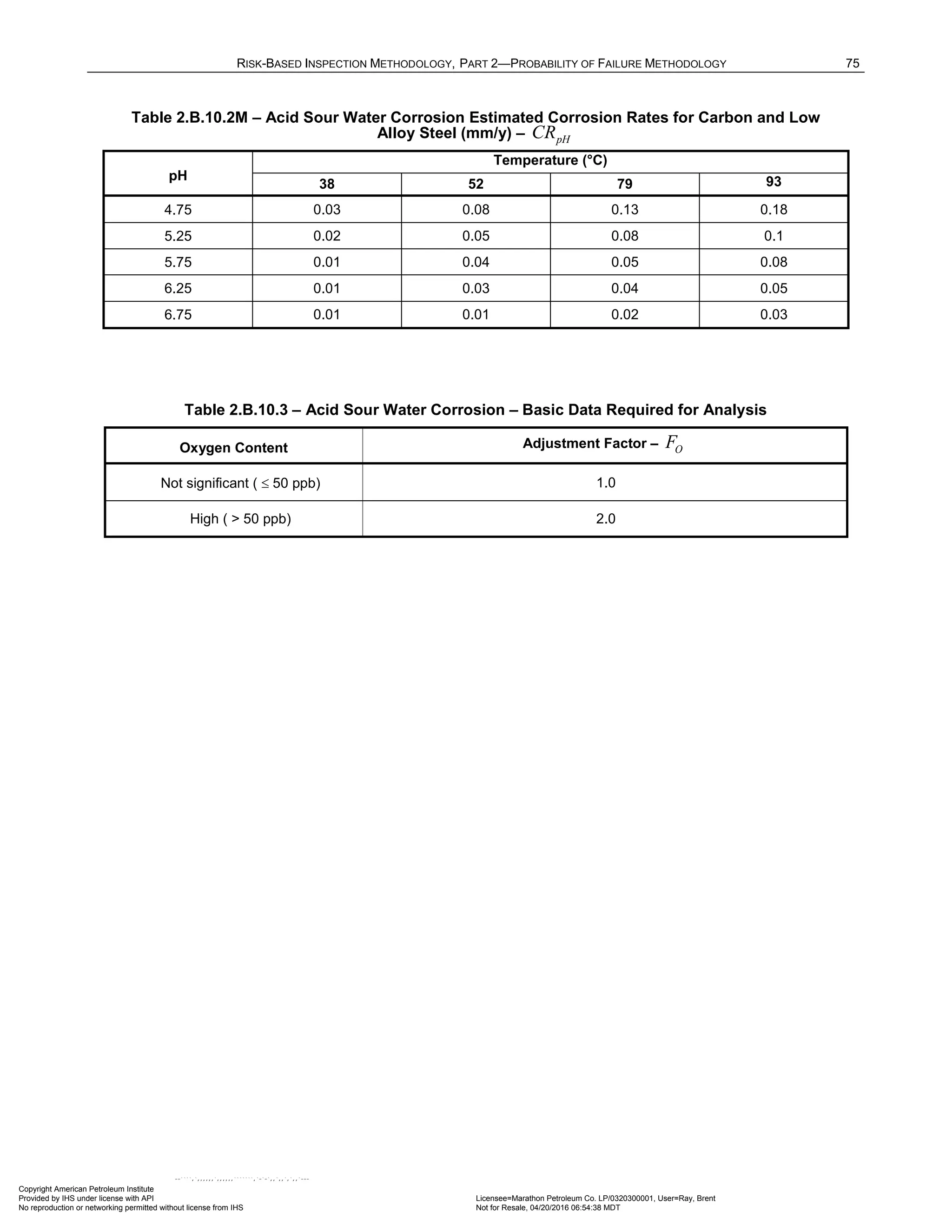
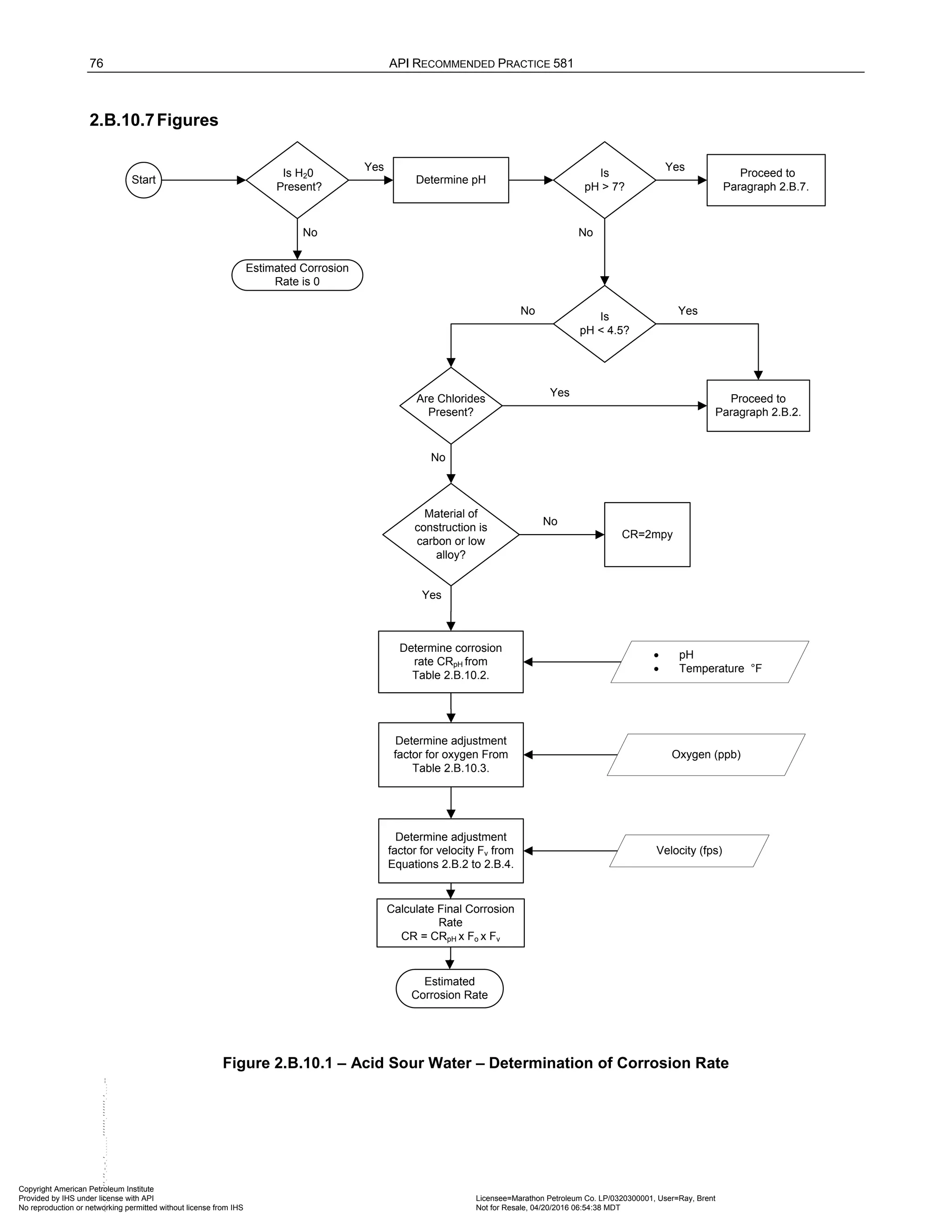
![RISK-BASED INSPECTION METHODOLOGY, PART 2—PROBABILITY OF FAILURE METHODOLOGY 77
2.B.11 Cooling Water Corrosion
2.B.11.1 Description of Damage
2.B.11.1.1 Overview
The objective for this paragraph is to describe a conservative approach for estimating corrosion rates of carbon
steel components in cooling water systems. In fresh water systems, a model uses the Ryznar Stability Index
(RSI), chloride content, temperature, and flow velocity to calculate a corrosion rate. For seawater systems, a
simple correlation of corrosion rate and velocity is used. Many other factors influence corrosion of the typical
modern cooling water system, and this paragraph also describes qualitatively some of these considerations.
This paragraph does not attempt to account for degradation of alloys other than carbon steel or to quantify the
effectiveness of water treatment. Many other alloys are used in cooling water systems. Some of these alloys
and the threats that they may face are described qualitatively, but corrosion rates of these alloys are assumed to
be very low. While low alloy steels are rarely used in cooling water systems, the corrosion rates given by this
methodology would be reasonably accurate for low alloy steels.
The best way to assess corrosion in cooling water systems is to use a variety of monitoring techniques, but
detailed use of those techniques is not described here. Most cooling water corrosion monitoring begins with the
use of corrosion coupons. Other techniques have been used to monitor cooling water corrosion in-situ, but they
are not described. Microbiologically-Induced Corrosion (MIC) is another common degradation mechanism in
cooling water systems, and coupons are not always a reliable way to monitor this corrosion or other corrosion
where there are deposits or stagnant areas. Direct monitoring and control of the microorganisms is
recommended.
2.B.11.1.2 Types of Cooling Water Systems
There are three types of cooling water systems typically found in industrial operations such as refineries:
a) Once through cooling – Does not reuse the heated water, which normally is pumped from a fresh water or
seawater source
b) Closed recirculating cooling – Continuously reuses water that is captive in the system. No make-up after the
initial water charge (except to replace accidental leakage).
c) Open recirculating cooling (cooling tower) – Reuses water from which the heat is rejected into a cooling
reservoir (tower or pond), needs continual make-up water to compensate for evaporation, blowdown, windage,
and drift losses, and needs a blow-down facility to limit the concentration of impurities that are typically
introduced with the make-up water.
2.B.11.1.3 Once Through Systems
Usually, the water source must be presumed corrosive since the surface waters are open to the atmosphere
and contain dissolved oxygen. In a general way, corrosion of iron and steel is proportional to the chloride
content when dissolved oxygen is constant, and vice versa. For seawater in particular, the flow velocity has a
significant impact on the corrosion rate.
Because once through cooling water is not reused, the volume of water circulated through such a system
effectively precludes chemical inhibition from a cost-effective standpoint. In some cases, a small amount of
scale inhibitor is added to the influent water. However, chlorination is usually necessary to control biological
growth (e.g., bacteria, slime, marine organisms).
Both fresh and saline waters are sufficiently corrosive to carbon steel that more corrosion-resistant materials
must be employed. In fresh water, galvanized steel is often adequate but brackish or salt water requires more
resistant materials (e.g., copper or nickel alloys; titanium; super-austenitic stainless steels [such as 6-Mo
stainless steels]; plastic; FRP or plastic-lined steel; concrete, etc.).
Copyright American Petroleum Institute
Provided by IHS under license with API Licensee=Marathon Petroleum Co. LP/0320300001, User=Ray, Brent
Not for Resale, 04/20/2016 06:54:38 MDT
No reproduction or networking permitted without license from IHS
--````,`,,,,,,`,,,,,,```````,`-`-`,,`,,`,`,,`---](https://image.slidesharecdn.com/api581-3rdedition-april2016-240227010601-3bf73ab5/75/Norma-API-581-3rd-Edition-April-2016-pdf-387-2048.jpg)
![RISK-BASED INSPECTION METHODOLOGY, PART 2—PROBABILITY OF FAILURE METHODOLOGY 81
a) Low alloy steels are rarely used in cooling water systems and will not be addressed in the remainder of this
paragraph. However, most of the content for carbon steel applies to low alloy steels.
b) This model does not consider degradation of alloys other than carbon steel. Beyond some general
comments, SCC and pitting of stainless steels and dealloying of copper alloys are not considered.
c) If coupon measurement results are available, these should be used instead of this model. As a rule of
thumb for carbon steel, the pitting rate is a factor of 5 to 10 times the coupon general corrosion rate,
(calculated by weight loss).
d) If corrosion inhibitors are being used, it is assumed that the program is designed and operated to
adequately control corrosion of carbon steel and alloy materials.
e) An effective microbiological control program is in place, and corrosion driven by MIC is negligible, i.e., can
be set to < 0.13 mm/y (5 mpy), pitting.
f) Water pH is kept within the range 6.5 to 9.5. Outside this pH range, the corrosion is assumed caused by
other means than what is covered in this paragraph.
g) In the event the RSI value is < 6, it is assumed that corrosion is retarded by scale formation, but can still be
estimated on the basis of the chloride content, temperature and flow velocity.
h) There is no deposition and no local low flow areas.
2.B.11.1.1 Corrosion Rates for Copper Alloys Components
This paragraph is not intended to cover material of construction other than carbon steel. The introduction of
other materials such as stainless steel, copper, nickel, zinc or aluminum-based alloys etc., might introduce other
types of degradation mechanisms. It is virtually impossible to model the complexity of the various materials and
interrelation with various chemical and contaminants in the water. Thus, it has been assumed that, in general,
the selection of appropriate alloy material combined with “correct” chemical treatment and process control will
render a negligible corrosion rate in the cooling water system.
In general, copper and its alloys are the most reliable and cost effective alloys for many water services, although
dezincification needs to be specifically inhibited for brasses containing more than 15% zinc. Copper, red brass,
inhibited admiralty brasses, aluminum brass, aluminum bronze, and cupronickels, in that order, are used for
water of increasing salinity and/or velocity. In the presence of dissolved oxygen, soft waters can be highly
corrosive to copper alloys. Also copper can suffer pitting under some conditions, which for fresh waters can be
described as three types of pitting:
a) Type 1 pitting is apparently caused by residual carbonaceous films from the manufacturing process;
b) Type 2 pitting is associated with hot soft waters (>60°C [140°F]), and
c) Type 3 pitting may occur in cold water or high pH and low salt concentrations, for unknown reasons.
Another issue related to copper alloys is cracking. Admiralty brass is very susceptible to ammonia SCC and
might experience SCC with only a trace amount of ammonia present.
An important factor for copper-based alloys is maintaining operation within design velocity limits. Velocities
under the lower limit can lead to increased deposition and underdeposit corrosion, and velocities exceeding the
upper limit can cause damage to the protective surface film resulting in impingement attack.
2.B.11.2 Basic Data
2.B.11.2.1 Recirculating Cooling Water Systems
The data listed in Table 2.B.11.1 is required for determining the estimated corrosion rate for recirculating cooling
water service. If precise data have not been measured, a knowledgeable process specialist should be
consulted.
2.B.11.2.2 Once Through Cooling Water Systems
The data listed in Table 2.B.11.2 is required for determining the estimated corrosion rate for once through
cooling water service. If precise data have not been measured, a knowledgeable process specialist should be
consulted.
Copyright American Petroleum Institute
Provided by IHS under license with API Licensee=Marathon Petroleum Co. LP/0320300001, User=Ray, Brent
Not for Resale, 04/20/2016 06:54:38 MDT
No reproduction or networking permitted without license from IHS
--````,`,,,,,,`,,,,,,```````,`-`-`,,`,,`,`,,`---](https://image.slidesharecdn.com/api581-3rdedition-april2016-240227010601-3bf73ab5/75/Norma-API-581-3rd-Edition-April-2016-pdf-391-2048.jpg)
![82 API RECOMMENDED PRACTICE 581
2.B.11.3 Determination of Corrosion Rate
2.B.11.3.1 Recirculating Cooling Water Systems
2.B.11.3.1.1 Corrosion Rate Equation
The steps required to determine the corrosion rate are shown in Figure 2.B.11.1. The corrosion rate is computed
using Equation (2.B.8). In this equation, the base corrosion rate, B
CR , is adjusted for temperature and flow
velocity for each component in the system to calculate a final representative corrosion rate.
= ⋅ ⋅
B T V
CR CR F F (2.B.8)
The estimated corrosion rates need further adjustments in case construction material is other than carbon steel.
This has not been addressed within this paragraph.
2.B.11.3.1.2 Base Corrosion Rate
The Base Corrosion Rate, B
CR , is an estimated corrosion rate that is determined from the water scale
tendency, chloride concentration, and a threshold for flow velocity (i.e., higher or lower than 2.44 m/s [8 ft/s]).
The concept of Ryznar stability indices is used to predict whether water variables in the pH range of 6.5 to 9.5
will produce conditions that are scaling or corrosive to carbon steel. The expected tendencies are increased
scaling conditions at higher temperatures, higher Ca hardness and higher MO Alkalinity and seeing corrosive
conditions at lower temperatures, lower Ca hardness or lower MO Alkalinity. MO Alkalinity refers to the Methyl
Orange and the test used to measure the total alkalinity of water.
For given values of calcium hardness, MO Alkalinity and total dissolved salt concentration, a value of pH ,
s
pH , exists at which the water is in equilibrium with solid CaCO3. The deposit of CaCO3 is thermodynamically
possible when the pH of water is higher than s
pH , i.e., higher than the pH at saturation of calcium
carbonate. The difference between the actual pH , a
pH , of a sample of water and the pH for CaCO3
saturated water, s
pH , is called the Langelier Saturation Index (LSI) and is computed using Equation (2.B.9).
s
a pH
pH
LSI −
= (2.B.9)
The Langelier Saturation Index is used to predict the tendency for CaCO3 to either dissolve or precipitate and
provide corrosion resistance in fresh water, under varying conditions.
While the concept of the Langelier index is correct and helpful; however, it should be emphasized that a positive
value of the index can result from waters of totally different quality. As the pH increases, the Ca2+
concentration decreases drastically. The corrosion protection characteristics of the resulting CaCO3 film differ
accordingly. In other words, waters of different pH , Ca hardness, and MO Alkalinity that give the same value
of the index have different corrosivity.
The Langelier index alone cannot be used to do any quantitative assessment. However when used along with
the Ryznar Stability Index (RSI) determined using Equation (2.B.10), a relatively good prediction of the scaling
or corrosive tendencies of a water is obtained.
2
=
⋅ −
s a
RSI pH pH (2.B.10)
This Ryznar Stability Index was developed based on actual operating results for waters with different saturation
indexes, and is used in practice for estimating corrosivity of water. The value of s
pH in Equation (2.B.10) is
calculated using Equation (2.B.11) and the parameters in Table 2.B.11.3.
Copyright American Petroleum Institute
Provided by IHS under license with API Licensee=Marathon Petroleum Co. LP/0320300001, User=Ray, Brent
Not for Resale, 04/20/2016 06:54:38 MDT
No reproduction or networking permitted without license from IHS
--````,`,,,,,,`,,,,,,```````,`-`-`,,`,,`,`,,`---](https://image.slidesharecdn.com/api581-3rdedition-april2016-240227010601-3bf73ab5/75/Norma-API-581-3rd-Edition-April-2016-pdf-392-2048.jpg)
![84 API RECOMMENDED PRACTICE 581
1 0.50 (3 )
V a
F V
= + ⋅ − for Va < 3 ft/s (2.B.16)
1
V
F = for 3 ft/s < Va < 8 ft/s (2.B.17)
1 0.25 ( 8)
V a
F V
=+ ⋅ − for Va > 8 ft/s (2.B.18)
This represents a fairly coarse and conservative way of factoring in the velocity effect in the corrosion rate
prediction model. In reality this effect is a product of a much more sophisticated interrelation between
temperature, dissolved oxygen, pH and velocity. However, the trend shown in Table 2.B.11.6 does comply with
actual testing described in [52] for velocities up to 2.13 m/s (7 ft/s). Note that for carbon steel in seawater, the
velocity is even more a governing factor for the corrosion rate.
2.B.11.3.2 Once Through Cooling Water Systems
2.B.11.3.2.1 Overview
The steps required to determine the corrosion rate are shown in Figure 2.B.11.1. Once through cooling water
systems are much less common in the US refinery industry than recirculation systems. Once through systems
may be economical where there is an abundance of surface water, but the effects of thermal pollution may be
too great to allow their use in some locations. Chemical treatment is normally environmentally unacceptable
and/or uneconomical. These systems rarely use anything but chlorination which controls biological growth.
It is assumed in this paragraph that chemical treatment is not applied and that the material of construction is
carbon steel. In practice, the materials of construction in once through systems may be copper alloys, titanium
alloys, stainless steels, PVC, cement-lined, or coated (organic) steel, or even galvanized carbon steel where the
supply source is known to be fairly clean fresh water.
The main concern for a once through cooling water system is the quality of the supply water, i.e., type of water
(sea or salt, brackish or fresh water) and level of contaminants (such as solids, phosphates, iron, ammonia,
bugs and bacteria, etc.). In total there are a large number of factors that ultimately affect damage to the
equipment in a once through cooling water system.
For simplicity of this corrosion model for once through systems, these systems are considered either as
seawater systems or fresh water systems, and the corrosion rates are determined as a function of temperature,
water flow velocity, dissolved oxygen and content of chlorides.
2.B.11.3.2.2 Fresh Water Once Through System
Fresh water comprises natural surface water with chloride content less than 1000 ppm. The corrosion rate is
estimated in the same manner as an open recirculating system, with no chemical treatment or corrosion
inhibition, except for biocide.
2.B.11.3.2.3 Seawater Once Through Systems
Seawater comprises brackish or seawater with a chloride content of more than 1000 ppm. The salts found in
seawater do not appreciably alter the pH value when dissolved in water. The main type of dissolved salt in
seawater is sodium chloride (NaCl).
Seawater typically contains about 3% sodium chloride with approximately 19,000 ppm chloride ion (and 11,000
ppm sodium). The chloride ions comprise about 55% of the Total Dissolved Solids (TDS). Dissolved Oxygen
(DO) is typically present at normal saturated values of 6 to 8 ppm at 24°C to 29°C (75°F to 85°F). The pH of
seawater is usually 7.7 to 8.3 in surface waters [44]. Seawater always contains SRB and a level of sulfate ion
concentration (2 to 3,000 ppm) conductive to SRB growth under anaerobic conditions. Anaerobic conditions will
exist under deposits (organic or inorganic), in crevices, and under the influence of BOD (Biological Oxygen
Demand) or COD (Chemical Oxygen Demand). One of the most important properties of seawater is its ratios of
concentrations of the major constituents are remarkably constant worldwide, including the level of chloride and
oxygen.
Copyright American Petroleum Institute
Provided by IHS under license with API Licensee=Marathon Petroleum Co. LP/0320300001, User=Ray, Brent
Not for Resale, 04/20/2016 06:54:38 MDT
No reproduction or networking permitted without license from IHS
--````,`,,,,,,`,,,,,,```````,`-`-`,,`,,`,`,,`---](https://image.slidesharecdn.com/api581-3rdedition-april2016-240227010601-3bf73ab5/75/Norma-API-581-3rd-Edition-April-2016-pdf-394-2048.jpg)
![RISK-BASED INSPECTION METHODOLOGY, PART 2—PROBABILITY OF FAILURE METHODOLOGY 85
The temperatures encountered in once through seawater systems usually preclude scale formation by inverse
solubility effects, which normally would initiate at about 88°C (190°F). Obviously deposits can occur under
extreme conditions of temperature in condensers, but this is an exceptional circumstance. Deposition of sand
and silt is primarily controlled by establishing a minimum flow and by mechanical cleaning as required.
Biofouling can be caused by soft organisms (slimes, algae and hydroids) and hard organisms (barnacles,
mussels, oysters, tubeworms and seasquirts). The degree of fouling depends to some extent on the material of
construction. Metals and alloys that produce toxic salts (e.g., copper, lead, and zinc) are more resistant. Both
fouling and bacterial effects are controlled largely by chlorination.
Corrosion of carbon steel in seawater is controlled by the availability of oxygen to the metal surface. Under static
conditions (zero velocity), carbon steel corrodes at rates between 0.10 and 0.20 mm/y (4 and 8 mpy), depending
on the local oxygen and temperature variations. As the velocity causes a mass flow of oxygen to the metal
surface, corrosion is very dependent on flow rate and can increase by a factor of 100 in moving from static
condition to a velocity of about 39.6 m/s (130 ft/s). Galvanizing confers only limited benefit under flow conditions,
as corrosion of zinc also increases with velocity. For the thickness normally used in seawater piping, it will
extend the life of the pipe for about 6 months only.
Thus, velocity is the most important single factor influencing design of carbon steel components in seawater
systems. The chosen design velocity controls the dimensions of many components, such as piping and valves.
When the corrosion rate is subject to mass transfer control, flow velocity at the metal surface becomes the rate-
determining factor.
Based on test results reported in [45,50,51]; Equations (2.B.19) and (2.B.20) may be used to compute the
corrosion rates on carbon steel in seawater systems as a function of the velocity, a
V . Values for the corrosion
rate as a function of velocity using this equation are shown in Table 2.B.11.7.
For SI Units, use Equation (2.B.19),
2 2.5
0.1318 0.3108 0.0579 .01208
a a a
CR V V V
= + ⋅ − ⋅ + ⋅ (2.B.19)
For US Customary units, use Equation (2.B.20).
2 2.5
5.1885 3.7293 0.21181 0.02439
a a a
CR V V V
= + ⋅ − ⋅ + ⋅ (2.B.20)
Equations (2.B.19) and (2.B.20) were developed based on the data specified in [50], assuming seawater
temperature of about 21°C (70°F) and an oxygen concentration of 6-8 ppm.
With high flow rates, the corrosion rate increases up to around 12.2 m/s (40 ft/s), where the attack changes to
erosion-corrosion. However, it is assumed that cooling water systems in the refining industry will not experience
water flow velocities in excess of 6.1 m/s (20 ft/s).
2.B.11.3.3 Ground Water
Ground waters are not specifically addressed in this paragraph. However, the following can be a quick guideline
for determining the level of corrosivity for such waters. The assessment needs to be made by a competent
person for water corrosivity issues.
Ground waters may contain well water, geothermal springs, or produced water (i.e., waters of brines co-
produced with oil or gas). Although ground waters can be considered one category, they might vary largely in
chemistry. Ground waters are often characterized in terms of Total Key Species (TKS), which is a sum of
chloride, sulfate, dissolved CO2, bicarbonate, carbonate, sulfide, and ammonia concentrations. TKS is a
measure of corrosivity. Depending on the TKS value, the corrosivity towards steel can be rated as:
a) Low (< 0.03 mm/y [1 mpy]) corrosion rate
b) Medium (0.03 to 0.25 mm/y [1 to 10 mpy])
c) High (0.25 to 1.27 mm/y [10 to 50 mpy])
d) Very High (> 1.27 mm/y [50 mpy])
The subject of specific TKS values versus corrosivity has not been addressed in this paragraph.
Copyright American Petroleum Institute
Provided by IHS under license with API Licensee=Marathon Petroleum Co. LP/0320300001, User=Ray, Brent
Not for Resale, 04/20/2016 06:54:38 MDT
No reproduction or networking permitted without license from IHS
--````,`,,,,,,`,,,,,,```````,`-`-`,,`,,`,`,,`---](https://image.slidesharecdn.com/api581-3rdedition-april2016-240227010601-3bf73ab5/75/Norma-API-581-3rd-Edition-April-2016-pdf-395-2048.jpg)
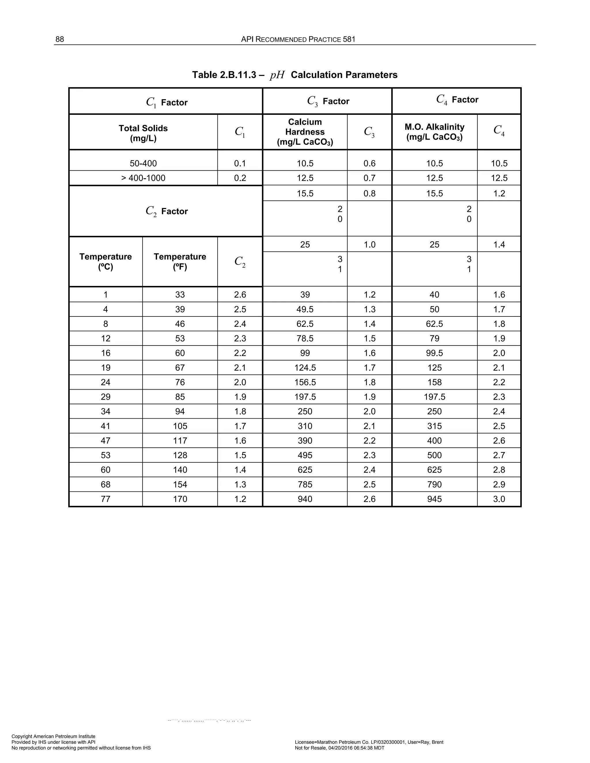
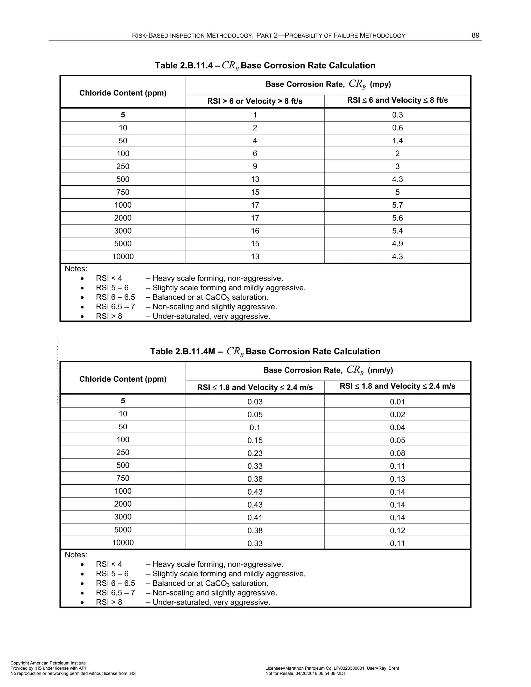
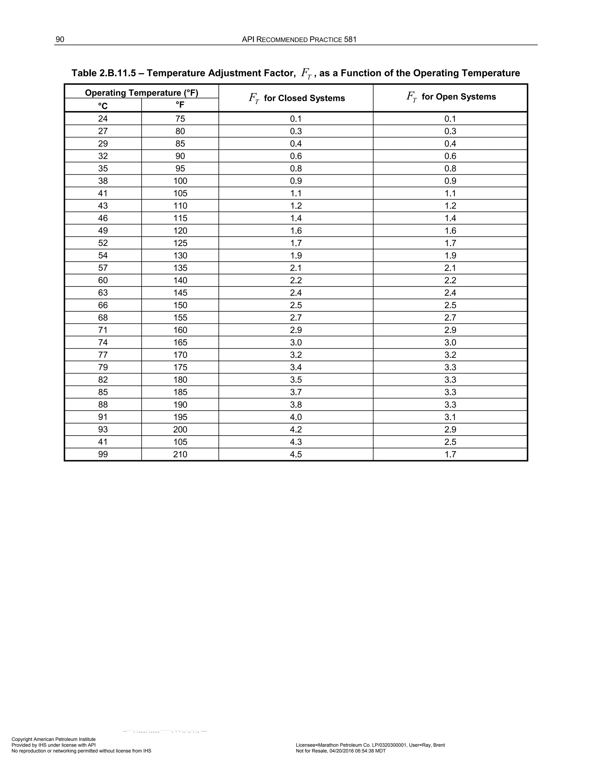
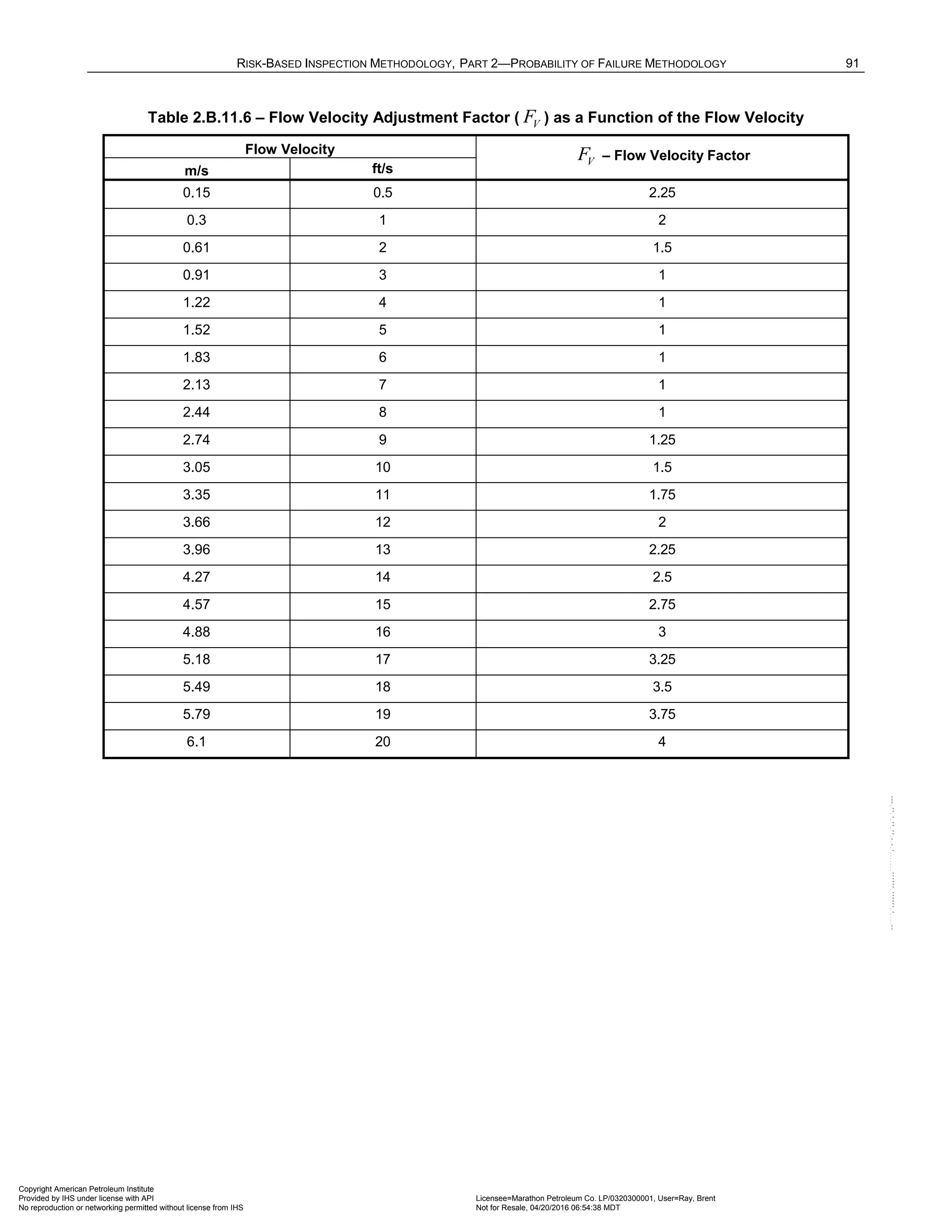
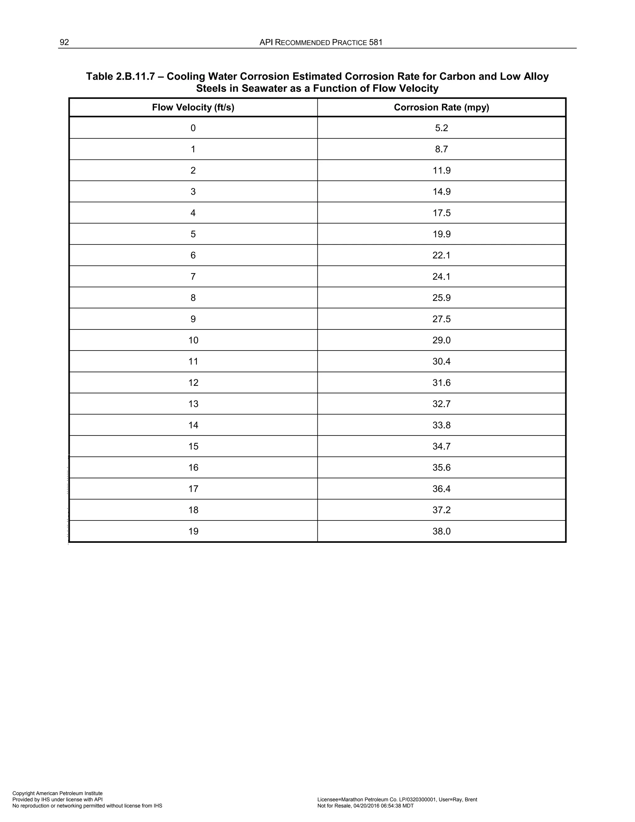
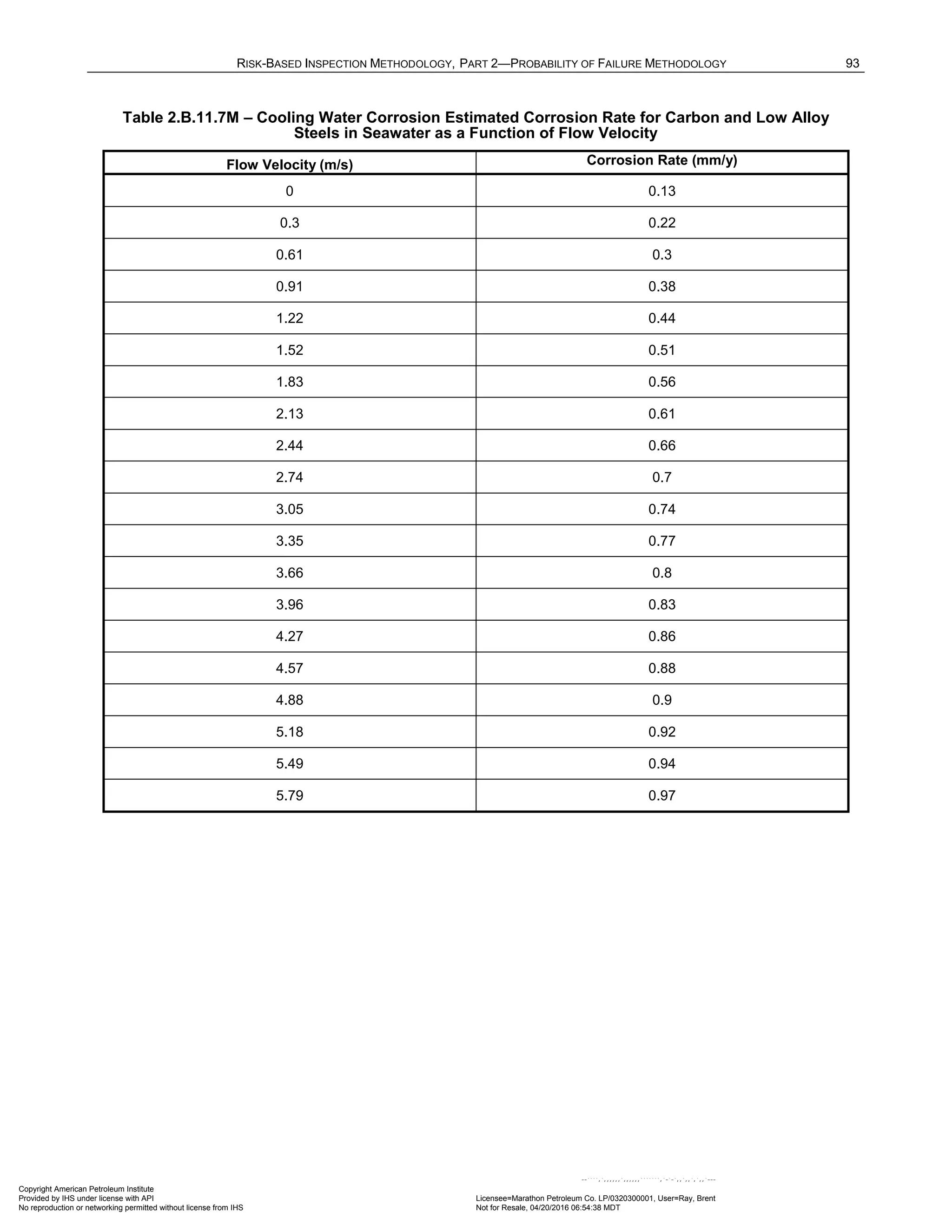
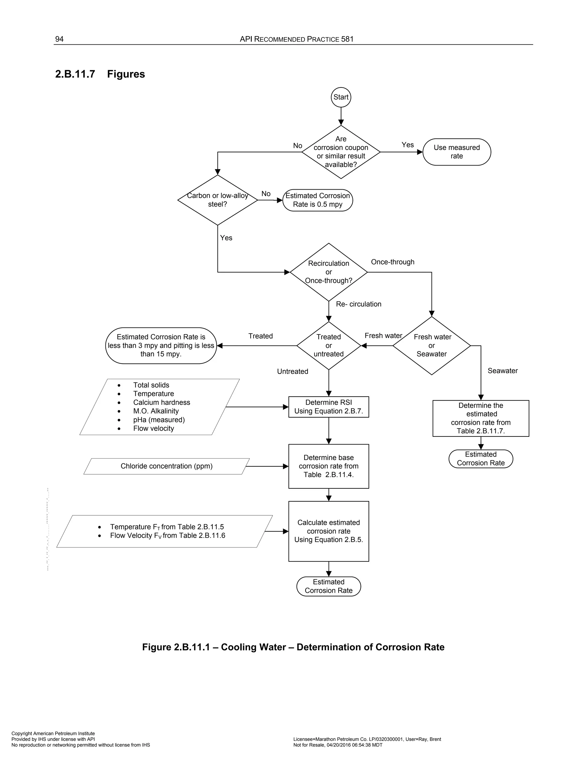
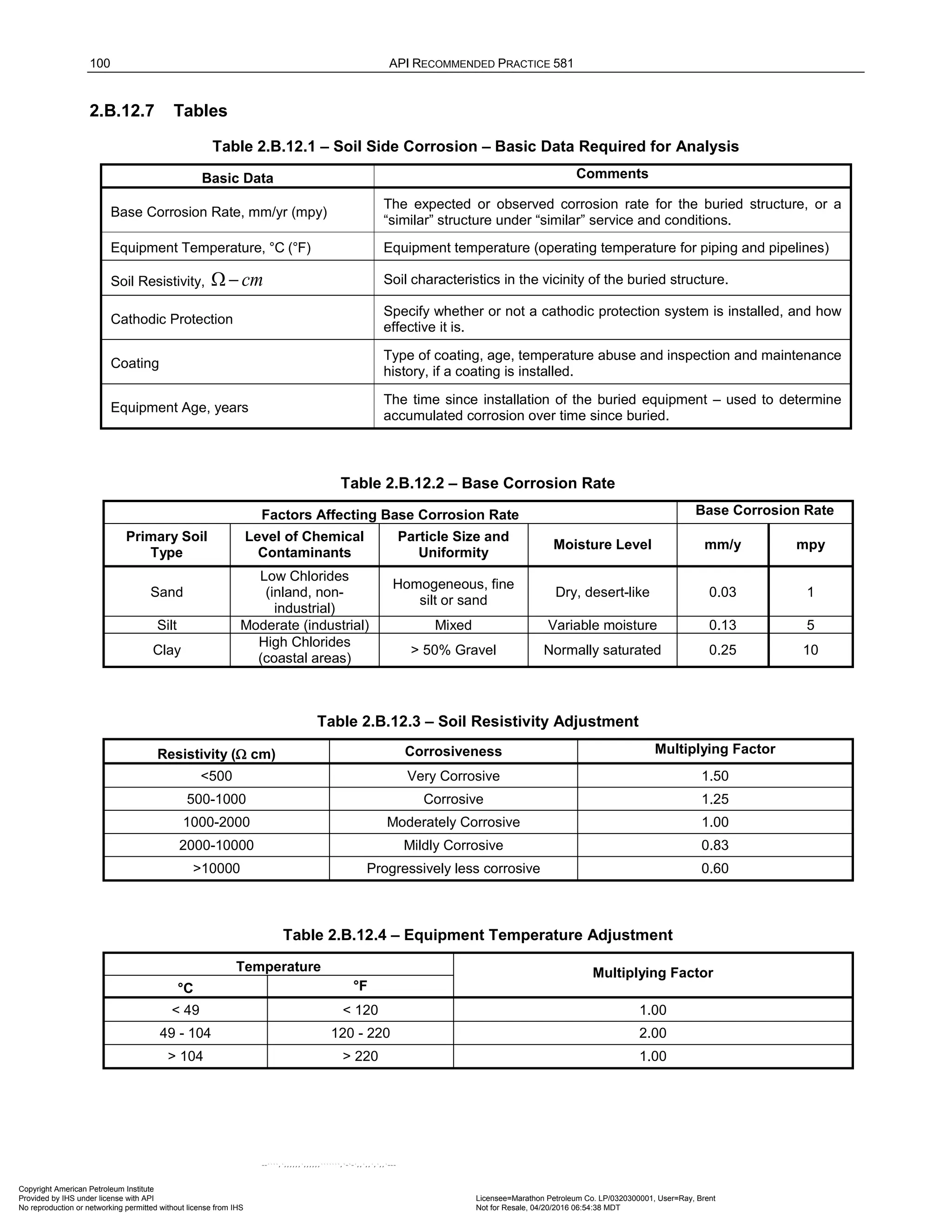
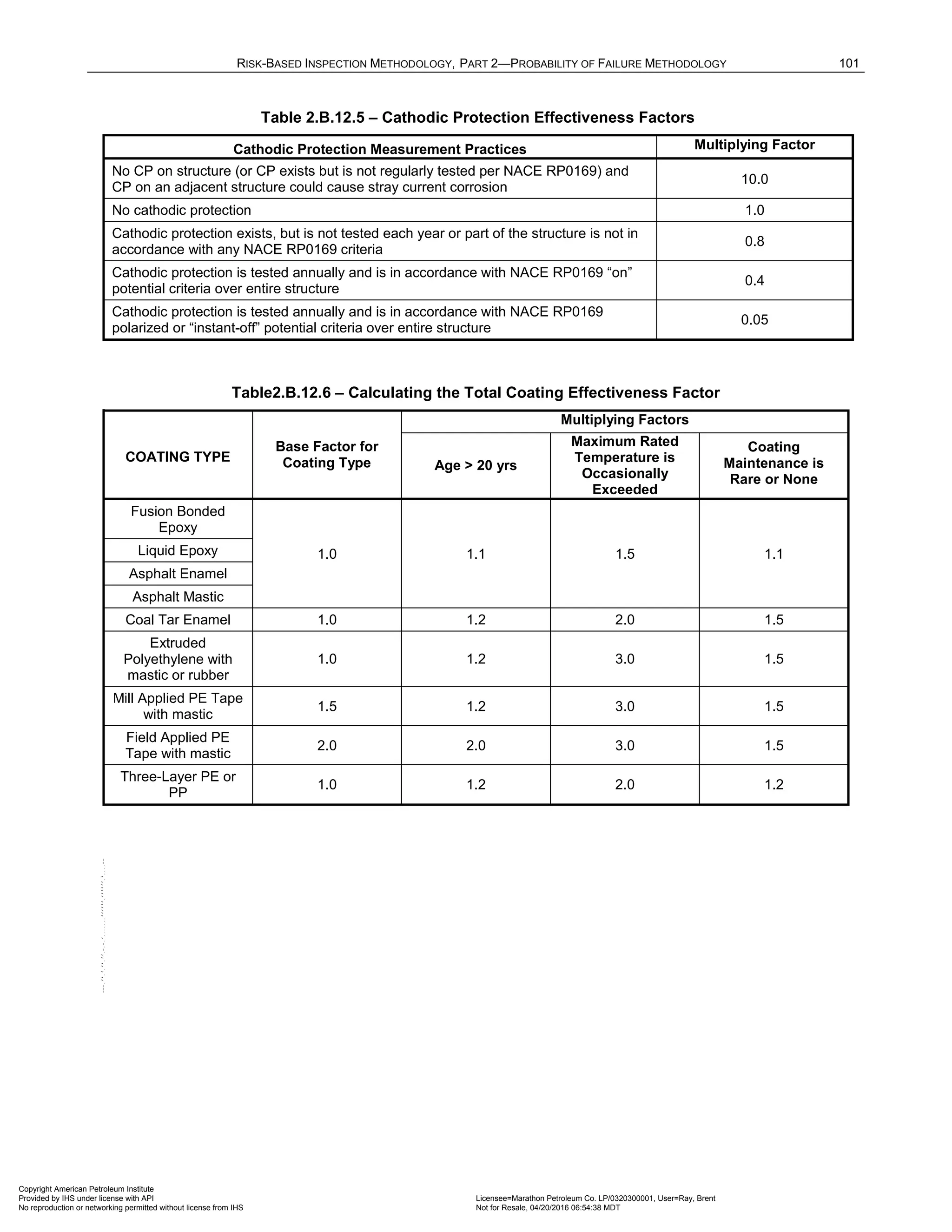
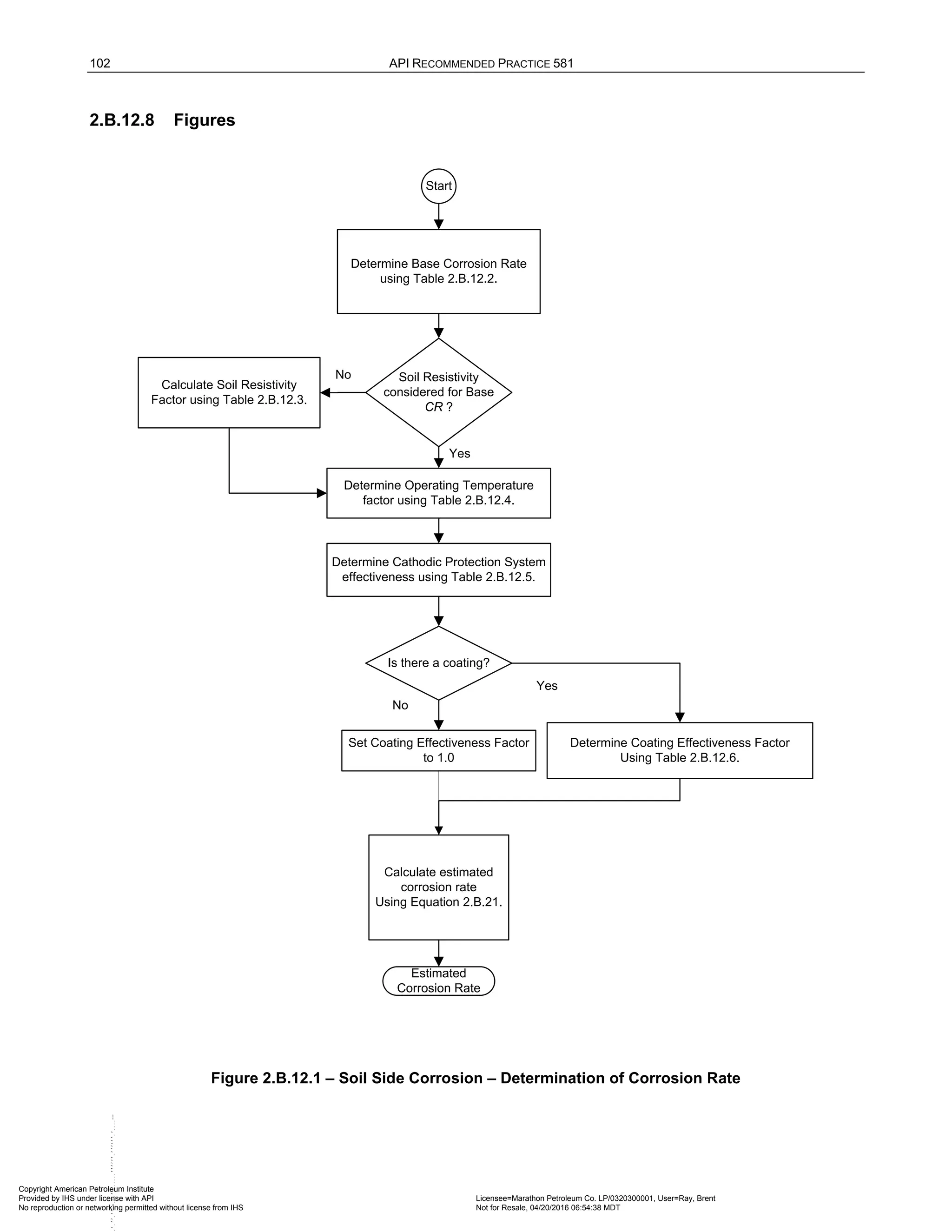
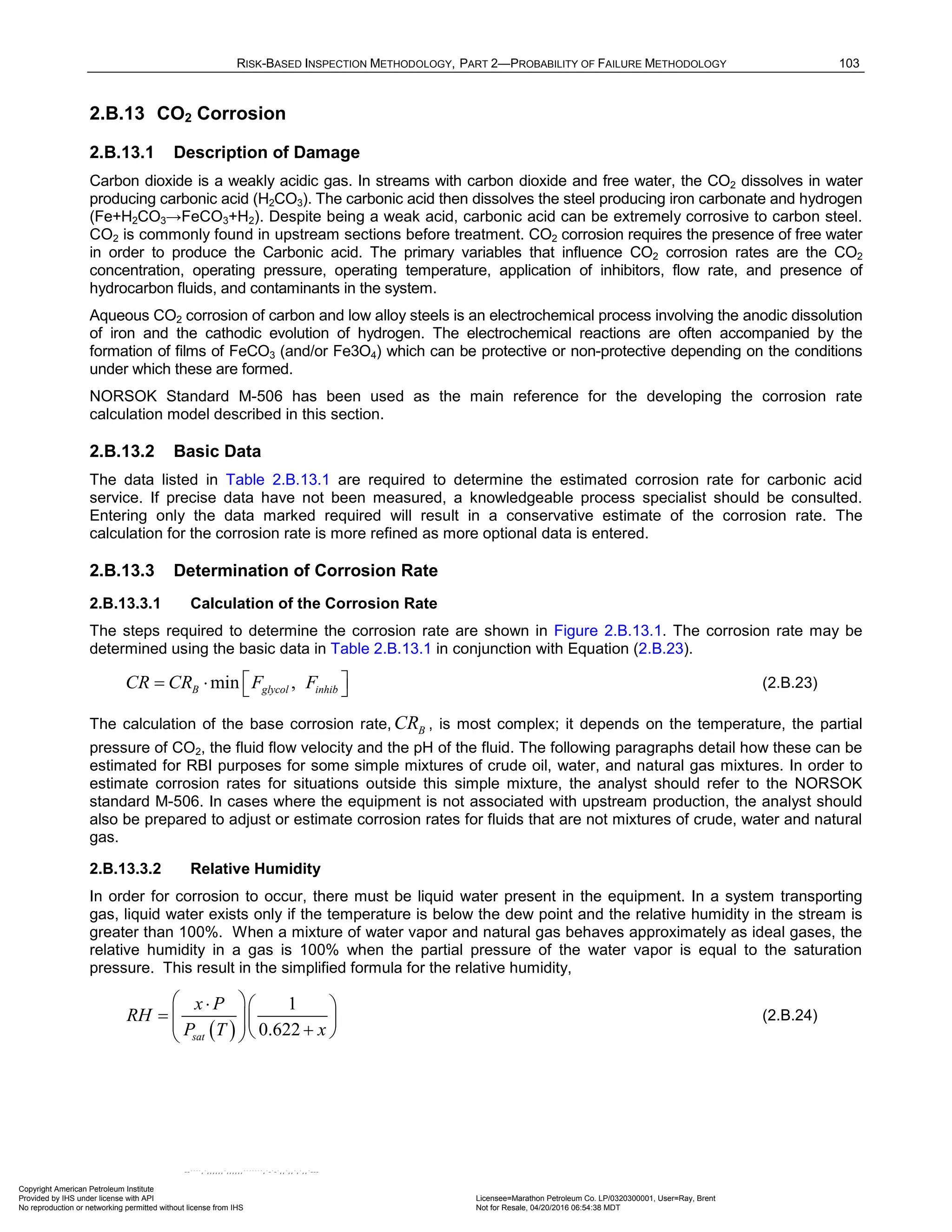
![104 API RECOMMENDED PRACTICE 581
In Equation (2.B.24), x is the ratio of the mass of water to the mass of dry gas, or ( )
% 100 %
w w
− , where
%wis the percent water by weight in the stream. The parameter P is the pressure and ( )
sat
P T is the
saturation pressure for water at temperature T , which can be obtained from steam tables. The 0.622 is the
ratio of the molecular weight of water (≈18) to the average molecular weight of air (≈29). Using Equation
(2.B.24) and standard steam tables, an approximate equation for the dew point temperature d
T (°F) can be
derived, see Equation (2.B.25).
[ ]
10 10 10
%
log 2.0866 0.2088 log 0.2242 log
100
d
w
T P
= + ⋅ + ⋅
(2.B.25)
In Equation (2.B.25), P is the pressure in psia, %w is the percent water by weight in the stream (lbm/100lbm),
between 0 and 30.
2.B.13.3.3 Base Corrosion Rate
The base corrosion rate in mm/y is calculated from Equation (2.B.26).To obtain mpy, multiply the result in mm/y
by 39.4.
( )
2
2
0.146 0.0324
0.62
,
19
CO
f
base CO
S
CR f T pH f
+
= ⋅ ⋅
(2.B.26)
In Equation (2.B.26), ( , )
f T pH is the temperature-pH function that is tabulated in Table 2.B.13.2. This
tabulated function was calculated by combining the M-506 temperature and temperature dependent function pH
function into a single quantity. It should be noted that the ( , )
f T pH function jumps sharply between 80°C and
90°C (176°F and 194°F.).
The CO2 fugacity, 2
CO
f in bar, pH, and the shear stress from the flow S in Pa needed to calculate the basic
corrosion rate are discussed in the following paragraphs.
2.B.13.3.4 Determining the pH
For RBI purposes, the pH term in temperature-pH function tabulated in Table 2.B.13.2 may be calculated using
one of the following approximations. For condensation,
[ ] 2
10 10
2.8686 0.7931 log 0.57 log CO
pH T p
= + ⋅ − ⋅ (2.B.27)
for Fe
++
saturated water,
[ ] 2
10 10
2.5907 0.8668 log 0.49 log CO
pH T p
= + ⋅ − ⋅ (2.B.28)
and for water with salinity slightly greater than seawater (salinity = 46 g/l),
[ ] 2
10 10
2.7137 0.8002 log 0.57 log CO
pH T p
= + ⋅ − ⋅ (2.B.29)
In Equations (2.B.27), (2.B.28), and (2.B.29), T is the temperature in °F and 2
CO
p is the CO2 partial pressure in
psi. These approximations were developed from Monte Carlo simulations. These simulation studies used the
equilibrium equations recommended and by M-506 to calculate the concentration of hydrogen cation and then
the pH for a wide range of temperatures, pressures, and CO2 mole fractions.
Equations (2.B.27), (2.B.28), and (2.B.29) apply to water, seawater and Fe
++
saturated water and do not account
for the buffering action of bicarbonate ions or for the increase acidity caused by salinity levels higher than 45 g/l.
In cases where these factors are significant, the analyst should consider using an alternative analysis such as
direct application of the provisions in M-506 for salinity and dissolved bicarbonate.
Copyright American Petroleum Institute
Provided by IHS under license with API Licensee=Marathon Petroleum Co. LP/0320300001, User=Ray, Brent
Not for Resale, 04/20/2016 06:54:38 MDT
No reproduction or networking permitted without license from IHS
--````,`,,,,,,`,,,,,,```````,`-`-`,,`,,`,`,,`---](https://image.slidesharecdn.com/api581-3rdedition-april2016-240227010601-3bf73ab5/75/Norma-API-581-3rd-Edition-April-2016-pdf-414-2048.jpg)
![RISK-BASED INSPECTION METHODOLOGY, PART 2—PROBABILITY OF FAILURE METHODOLOGY 105
2.B.13.3.5 Determining the CO2 Fugacity
Fugacity has units of pressure. It is used in place of the pressure – or partial pressure – in calculations
concerning the equilibrium of real gas mixtures. When the fugacity is used in place of the pressure, real gases
can be modeled using the equations for ideal gases. M-506 uses the following equation for modeling the
fugacity, 2
CO
f .
2 2 2
10 10
1.4
log log min 250, 0.0031
273
CO CO CO
f p p
T
= + ⋅ −
+
(2.B.30)
[ ]
2 2
10 10 10
log log log
CO CO
f p a
= +
(2.B.31)
In Equations (2.B.30) and (2.B.31), 2
CO
p is the CO2 partial pressure in bar and T is the temperature in °C.
Note that the fugacity coefficient, a , is the ratio between CO2 fugacity and the partial pressure, or:
2 2
CO CO
f p a
= ⋅ (2.B.32)
2.B.13.3.6 Determining the Flow Velocity
M-506 uses the fluid flow shear stress to model the effect of flow velocity on the base corrosion rate. M-506
recommends the Equation (2.B.33) to calculate the stress, S , in units of Pa. In the calculation for the corrosion
rate, the shear stress need not exceed 150 Pa.
2
2
m m
f u
S
ρ
⋅ ⋅
= (2.B.33)
In Equation (2.B.33), f is the friction factor, m
u is the mixture flow velocity in m/s, and m
ρ is the mixture mass
density in kg/m
3
. The friction coefficient may be approximated for turbulent flow (Re > 2300) by using Equation
(2.B.34).
0.33
6
10
0.001375 1 20000
e
f
D Re
= + +
(2.B.34)
The term e D is the relative roughness and Re is the Reynolds Number of the mixture given by Equation
(2.B.35).
m
m
m
m
A
D
m
u
D
Re
m
m
ρ
=
= (2.B.35)
In Equation (2.B.35), D is the diameter in meters, and m
m is viscosity of the mixture in Pa·s (0.001cP = Pa·s).
This equation also shows that the Reynolds number can be calculated using the mass flux, m
, and the cross
sectional area, A .
M-506 gives some guidance on the calculation of the two-phase viscosity, density, and fluid velocity. These
factors depend on the volumetric ratio of the liquid flow to the flow, sometimes known as the liquid hold up, the
amount of water in the liquid fraction, the gas water and oil viscosities at the temperature and pressure. These
calculations are complex and go beyond the scope of an RBI study. If required, the analyst can refer to the
recommendations in NORSOK or use the software provided by NORSOK to perform the calculations
recommended in M-506 to approximate the two-phase flow characteristics. While M-506 provides some
guidelines for the calculation of bulk fluid properties, they do not explicitly account for the solubility of natural gas
in oil, which can also affect the all of these properties.
Copyright American Petroleum Institute
Provided by IHS under license with API Licensee=Marathon Petroleum Co. LP/0320300001, User=Ray, Brent
Not for Resale, 04/20/2016 06:54:38 MDT
No reproduction or networking permitted without license from IHS
--````,`,,,,,,`,,,,,,```````,`-`-`,,`,,`,`,,`---](https://image.slidesharecdn.com/api581-3rdedition-april2016-240227010601-3bf73ab5/75/Norma-API-581-3rd-Edition-April-2016-pdf-415-2048.jpg)
![106 API RECOMMENDED PRACTICE 581
2.B.13.3.7 Adjustment for Inhibitors or Glycol
The addition of glycol reduces the CO2 corrosion rate. M-506 accounts for this by simply reducing the corrosion
rate by applying a factor of the form:
[ ]
( )
10
log 1.6 log 100 2
glycol
F G
= ⋅ − −
(2.B.36)
In Equation (2.B.36), G is the percent weight of glycol as a percent of water in the system. glycol
F is limited to a
minimum value of 0.008. The base corrosion rate is multiplied by the factor glycol
F to account for the corrosion
reduction due to glycol.
For other types of corrosion inhibitors added to the stream, M-506 requires that its effectiveness must be
independently determined and used directly as a reduction factor, inhib
F . If both glycol and an inhibitor are used,
the minimum of inhib
F and glycol
F should be used as shown in Equation (2.B.23).
2.B.13.4 Nomenclature
a is the fugacity coefficient
A is the pipe cross sectional area, m
2
[ft
2
]
CR is the corrosion rate
B
CR is the base corrosion rate
D is the pipe diameter, m [ft]
e D is the relative roughness
f is the fraction factor
2
CO
f is the CO2 fugacity, bar
( , )
f T pH is the temperature-pH function
glycol
F is the corrosion rate correction factor for glycol
inhib
F is the corrosion rate correction factor for the inhibitor
G is the percent weight of glycol as a percent of water in the system
m
is the calculated using the mass flux, kg/m
2
-s [lb/ft
2
-s]
P is the pressure, psia
( )
sat
P T is the saturation pressure for water at temperature T , psia
2
CO
p is the CO2 partial pressure, bar [psi]
%w is the percent water by weight in the stream
Re is the Reynolds Number
RH is the relative humidity
m
ρ is the mixture mass density, kg/m
3
S is the shear stress, Pa
T is the temperature, °C [°F]
d
T is dew point temperature, °C [°F]
m
u is the mixture flow velocity, m/s
m
m is the viscosity of the mixture, cp
x is the ratio of the mass of water to the mass of dry gas
Copyright American Petroleum Institute
Provided by IHS under license with API Licensee=Marathon Petroleum Co. LP/0320300001, User=Ray, Brent
Not for Resale, 04/20/2016 06:54:38 MDT
No reproduction or networking permitted without license from IHS
--````,`,,,,,,`,,,,,,```````,`-`-`,,`,,`,`,,`---](https://image.slidesharecdn.com/api581-3rdedition-april2016-240227010601-3bf73ab5/75/Norma-API-581-3rd-Edition-April-2016-pdf-416-2048.jpg)