(New) Borders for Quantum Cosmology

Paulo Vargas Moniz; Vitória / Rio de Janeiro - 2011 Quantum Cosmology - p. 1
(NEW) BORDERS FOR QUANTUM COSMOLOGY
Standpoint and (some) SUSY
LNP 803 - 804, Springer, 2010
Paulo Vargas Moniz(1)
(1) UBI & CENTRA-IST,

Abstract
Quantum Cosmology tackles the quantum description of the
early universe. It is aimed as an accessible primer that covers
the basics, critically discussing ideas and concepts that
comprise our current knowledge. The scope for analyzing
quantum cosmological models within a supersymmetric
framework is pointed.
As much as possible, it summarizes what we know, what we
think we know and what we think we do not know on an equal
footing. It is focused for ‘young’, inquisitive minds eager to
embark on in-depth research in this ﬁeld. It is hoped to suggest
the tools researchers will need to go on their own, pushing
them to ask the right questions rather than seek deﬁnitive
answers.

N=2 SUSY

QC SUSY part-I
■ Starting from
■ bosonic conﬁgurations
■ General Relativity or bosonic sector (strings)
■ Setting:
ds2
= −N2
(t)dt2
+ hij(t)ωi
ωj
hij(t) =
1
6π
e2α(t)
e2β
(t) ij
=
1
6π
e2βi
δij,
βij(t) ≡ diag(β+ +
√
3β−, β+ −
√
3β−, −2β+)

QC SUSY part-I
■ Hamiltonian
H =
1
2
(−p2
α + p2
+ + p2
−) + U(0)
(α, β+, β−)
=
3
2
(p1)2
+ (p2)2
+ (p3)2
− 2p1p2 − 2p1p3 − 2p2p3
+ U(0)
(β1
, β2
, β3
), (1)
■ U(0)
≡ −12π2
h(3)
R
type I : U
(0)
I ≡ 0 (2)
type II : U
(0)
II ≡
1
6
e4α
e−8β+
=
1
6
e4β3
, (3)
type IX : U
(0)
IX ≡
1
6
e4α
2e4β+
(cosh(4
√
3β−) − 1) + e−8β+
−4e−2β+
cosh(2
√
3β−)
=
1
6
e4β1
+ e4β2
+ e4β3
− 2e2β1
+2β2

QC SUSY part-I
■ Hidden supersymmetry (SUSY)
■ Retrieved when potential U(q) is derivable from a
superpotential W(q)
■
U(q) =
1
2
GXY
(q)
∂W(q)
∂qX
∂W(q)
∂qY
,
■ Hamilton-Jacobi equation
■ Euclidean time
■ Euclidean action

QC SUSY part-I
■ Superpotentials W
◆ Bianchi type I:
WI ≡ 0;
◆ Bianchi type II:
WII ≡
1
6
e2α−4β+
=
1
6
e2β3
;
◆ Bianchi type IX:
W
(0)
IX ≡
1
6
e2α
2e2β+
cosh 2
√
3β− + e−4β+
=
1
6
e2β1
+ e2β2
+ e2β3
; (1)

QC SUSY part-I
■ Classical Hamiltonian
Hc =
1
2
GXY
(q) pX pY +
∂W
∂qX
∂W
∂qY
.
■ Quantum Hamiltonian H,
2H = ˜SS + S ˜S
■ where S, ˜S are linear operators satisfying
S2
= 0 = ˜S2
.

QC SUSY part-I
■ The operators S and ˜S have the explicit form
S ≡ ψx
ex
Y
(q) πY + i
∂W
∂qY
(1)
˜S ≡ ¯ψxexY
(q) πY − i
∂W
∂qY
, (2)
■ ex
Y
(q) ≡ e−Ω
δY
x is the minisuperspace vielbein associated
with GXY
(q)
■ They satisfy ex
Y
(q)ey
X
(q)ηxy
≡ GXY
(q),

QC SUSY part-I
■ ηxy
is the local ‘Lorentz’ metric at the minisuperspace
tangent section.
■ The ψx
and their adjoint ¯ψx are fermionic operators,
■ constituting Grassmannian (odd) partners of the qX
,
■ Therefore: introducing fermionic (!) minisuperspace
degrees of freedom and enlarging the (minisuperspace)
conﬁguration space,
■ satisfying
{ψx
, ψy
} = 0 = ¯ψx, ¯ψy (1)
ψx
, ¯ψy = δx
y . (2)

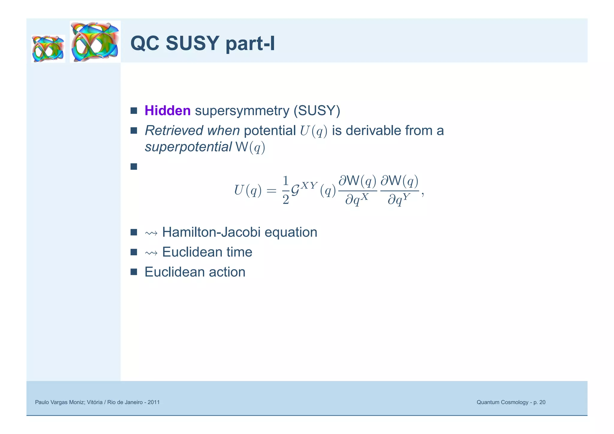
QC SUSY part-I
■ Hamiltonian
H = −
2
2 GXY ∂
∂qY
∂
∂qX + 1
2 GY X ∂W
∂qY
∂W
∂qX
+2 ex
Y
ey
X ∂2
W
∂qY ∂qX [ ¯ψx
, ψy
]
;
■ Fermion number
F ≡ ¯ψxψx
■ Conserved:
■
[H, F] = 0, [S, F] = S, [ ˜S, F] = − ˜S.

SQC and SUGRA

SQC SUGRA
■ Important “section”...
■ ... reduction of 4-dimensional canonical quantum N = 1
SUGRA
■ E.g., FRW models:
■ simplest
■ ‘bottom-up’
■ (prudent) approach on (i) how SQC research should
proceeded, (ii) methods that are to be applied and (iii) the
results retrieved: general? Useful?
■ FRW Minisuperspace Reduction Ansätse: Consistent with
■ supersymmetry,
■ Lorentz
■ general coordinate transformations,
■ Purpose: minisuperspace that will inherit invariance under
local time translations, supersymmetry and Lorentz
transformation.

SQC SUGRA
■ Tetrad and Gravitino Ansätze:
■ Closed (k = +1) FRW universes have S3
spatial sections.
■ Tetrad eAA
µ = ea
µσAA
a (in 2-spinor notation)
eaµ =
N(τ) 0
0 a(τ)eˆai
, eaµ
=
N(τ)−1
0
0 a(τ)−1
eˆai
,
■ For ψA
µ and ¯ψA
µ
■ ψA
0 and ¯ψA
0 to be functions of time only.
■ Furthermore
ψA
i = eAA
i
¯ψA , ¯ψA
i = eAA
i ψA ,

SQC SUGRA
■ Action:
■ integration over the spatial hypersurfaces
■ minisuperspace with N = 4 local supersymmetry and
time-invariance reparametrization
■ (obvious!) Elimination of (the presence) of spatial indices by
contraction.
■
Lfree = −
3a
N
˙a −
i
4
¯ψ0A
¯ψA
− ψA
ψ0A
2
−i
3
2
a3
nAA ψA ¯ψA
− i
3
2
a3
nAA
¯ψA ˙ψA
+ 3Na
+
3
2
a2 ¯ψ0A
¯ψA
+ ψA
ψ0A −
3
2
Na2
nAA
ψA
¯ψA
+
3
16
a3
nAA ¯ψ0A ψA
¯ψB ¯ψB + ψ0A
¯ψA ψB
ψB .(2)

SQC SUGRA
■ Hamiltonian
H = NH + ψA
0 SA + ¯SA
¯ψA
0 + MAB
JAB + ¯MA B ¯JA B ,
■ ψA
0 , ¯ψA
0 together with MAB
, ¯MA B
are Lagrange
multipliers.
■ H⊥ ≡ H Hamiltonian constraint, SA, ¯SA and JAB, ¯JA B
denote, respectively, the supersymmetry and Lorentz
constraints
■ Full set of constraints takes a rather simple form
SA = ψAπa − 6iaψa, (2)
H = −a−1
(π2
a + 36a2
), (3)
¯SA = ¯ψA πa + 6ia ¯ψA , (4)
JAB = ψ(A
¯ψB
nB)B . (5)

SQC SUGRA
■ E.g., Quantum States for the Vacuum Case
■ Momentum variables are represented as
¯ψA →
∂
∂ψA
, πa → −i
∂
∂a
.
■ SUSY constraints:
SA = −
1
2
√
3
aψA
∂
∂a
−
√
3a2
ψA,
¯SA =
1
2
√
3
a
∂
∂a
∂
∂ψA
−
√
3a2 ∂
∂ψA
. (2)
■ Lorentz:
JAB = ψ(A
∂
∂ψB)
.

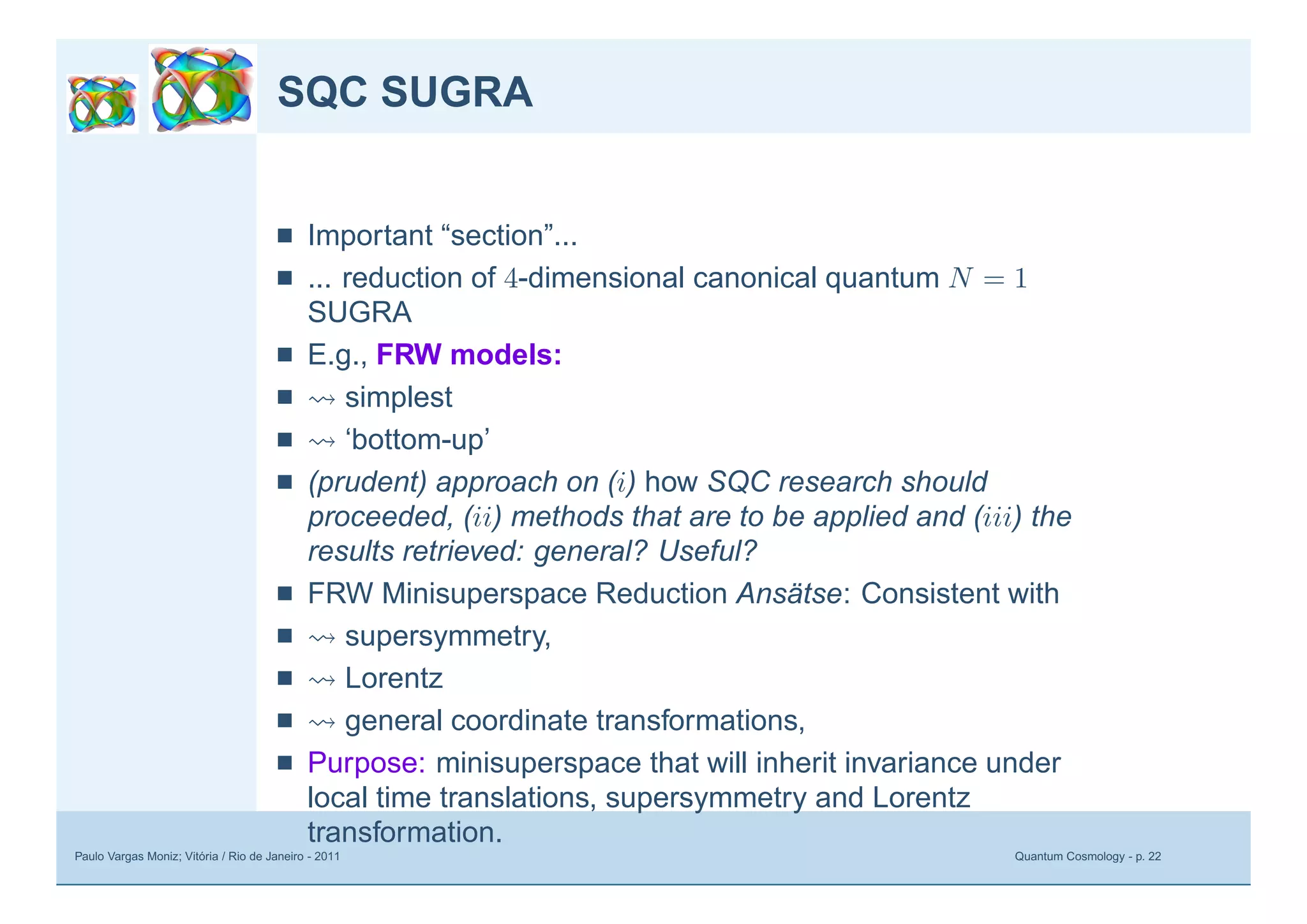
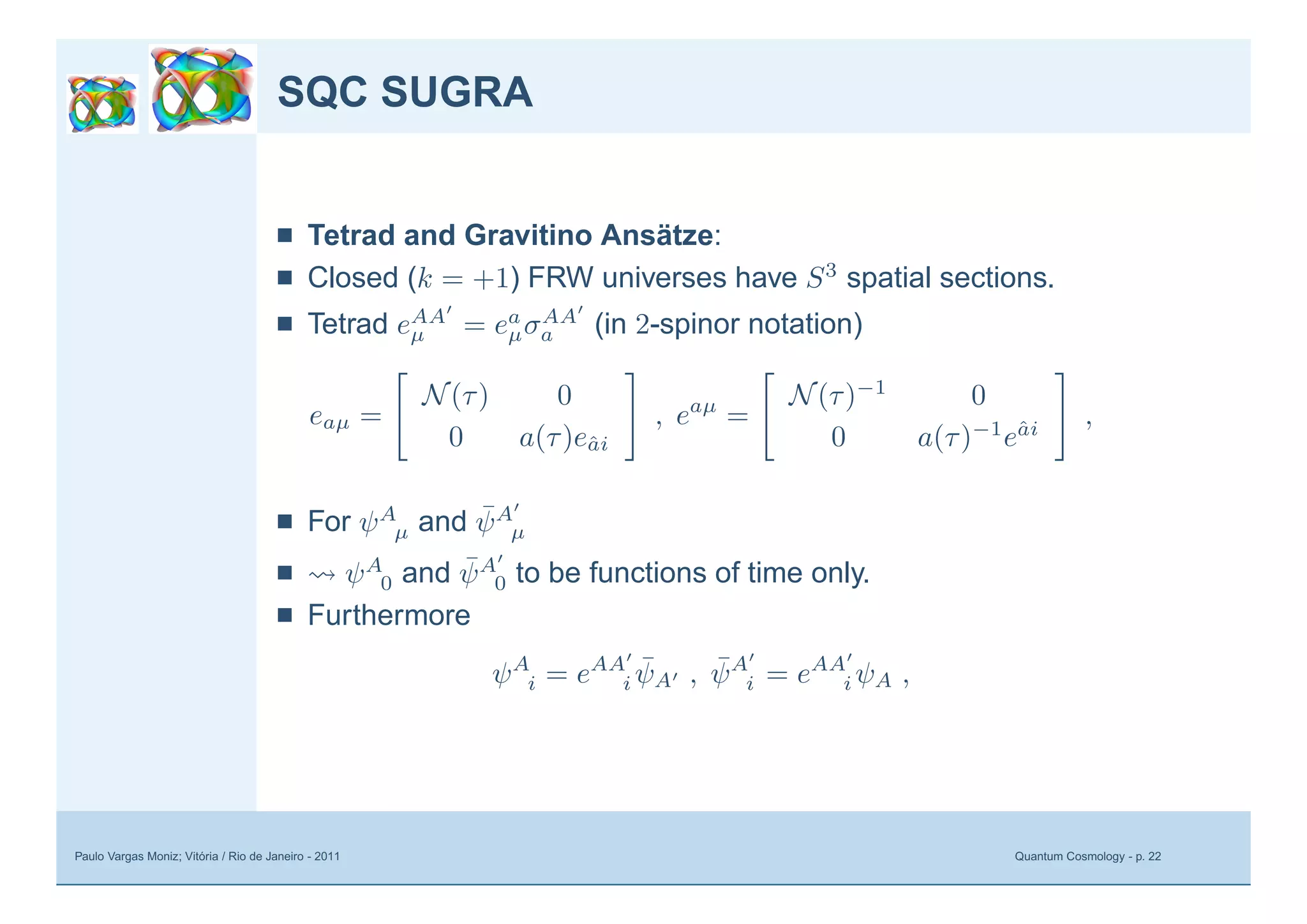
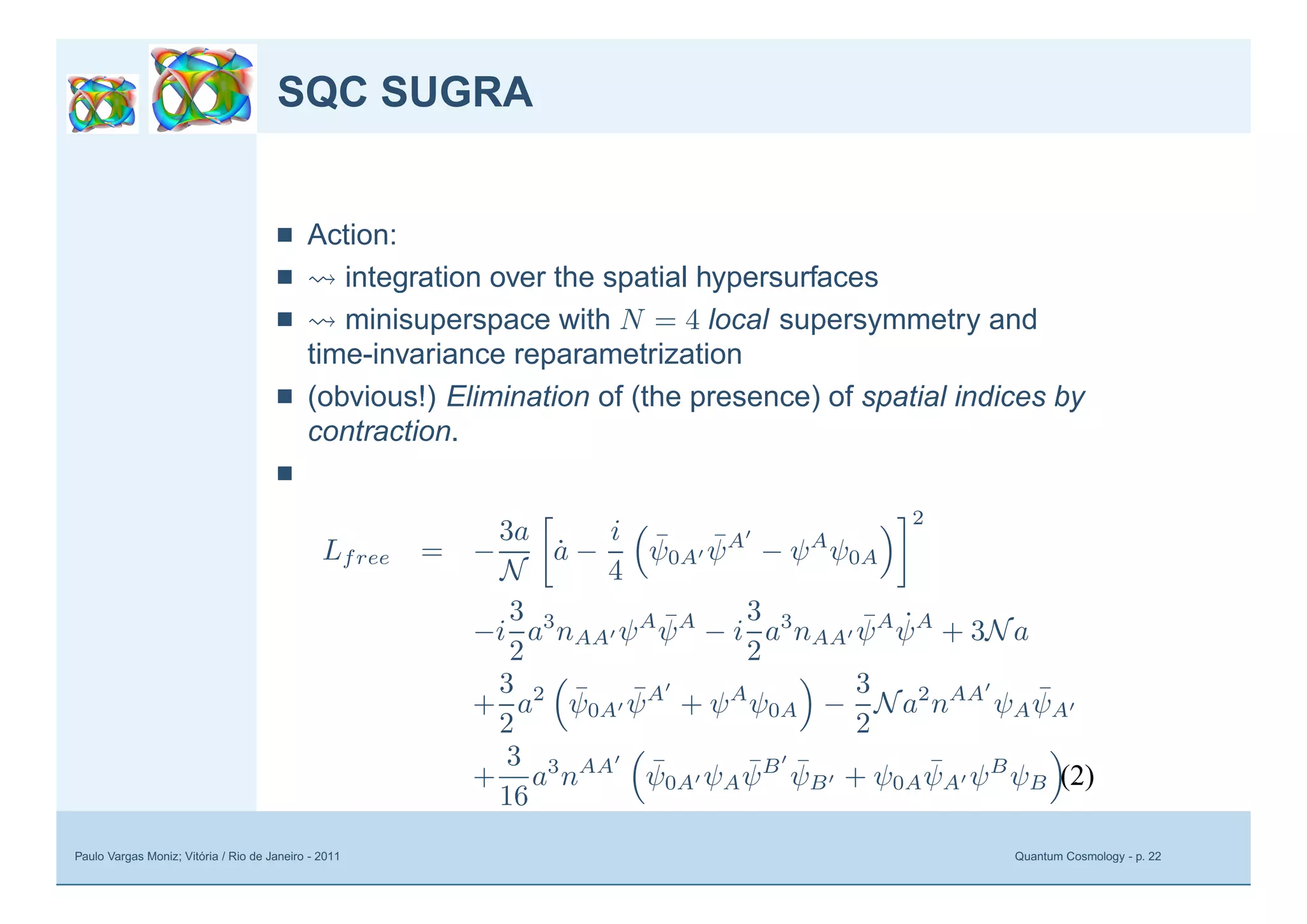
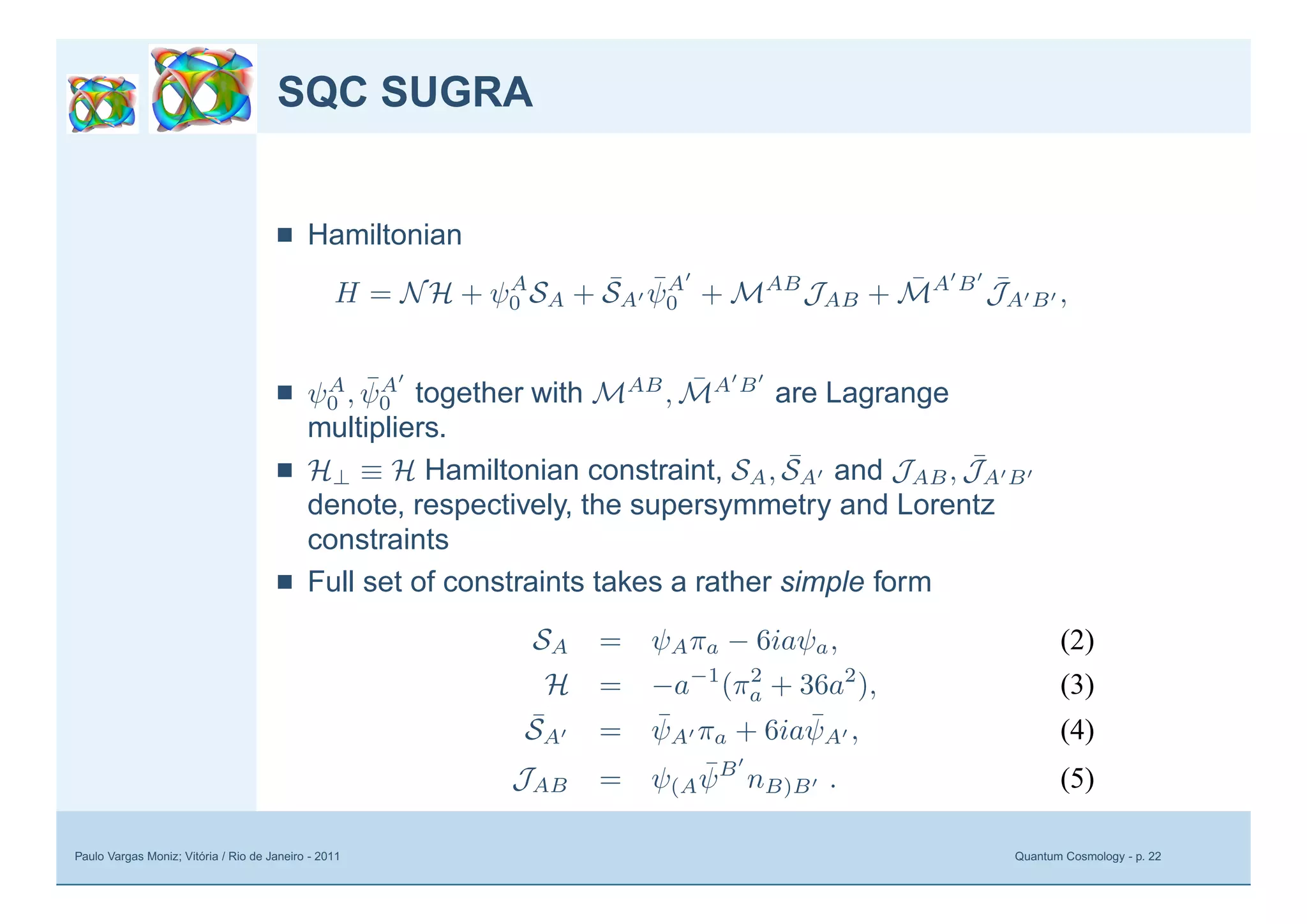
SQC SUGRA
■ Wave function:
ΨF RW
SUSY = A(a) + B(a)ψF
ψF . (2)
■ Equations to solve: SAΨ = 0, ¯SAΨ = 0
a
√
3
∂aB − 2
√
3a2
B = 0,
a
√
3
∂aA + 2
√
3a2
A = 0.
■ Solutions are
Ψ = A0 exp[−3a2
/ ] + B0 exp[3a2
/ ]ψAψA
,
■ A0 and B0 are independent of a and ψA
.
■ Semi-classical interpretation as exp(−I/ )
■ I.e., we get a Hartle–Hawking solution for B = 0

Can it be real?!

Semiclassical Expansion
■ ... if (and how) our physical (observed) universe can be
retrieved from SQC physical states

For Research...

Outlook yet again...
■ So,
1. How can the ‘hidden’ N = 2 SUSY be retrieved?
2. And what about when (super)matter includes a scalar
ﬁeld or a Yang–Mills sector?
3. How precisely can we implement a FRW SQC
(minisuperspace) from N = 1 SUGRA?
4. How can scalar (super)matter be included?
5. Why is the case of Bianchi models with a cosmological
constant still an issue?
6. How does the DeWitt supermetric relates to the usual
DeWitt metric?
7. What are the main features of SUGRA (quantum)
corrections into the Schrödinger equation?
8. Can SQC become ‘observational’?

(New) Borders for Quantum Cosmology

More Related Content

What's hot

Similar to (New) Borders for Quantum Cosmology

More from Paulo Vargas Moniz

Recently uploaded

(New) Borders for Quantum Cosmology