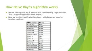
Naive Bayes is a simple classification technique based on Bayes' theorem that assumes independence between predictors. It works well for large datasets and is easy to build. Some key points:
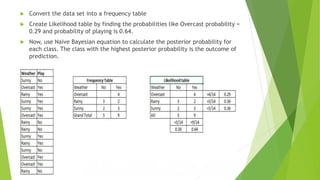
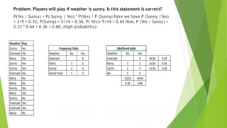
- It calculates the probability of class membership based on prior probabilities of classes and predictors.
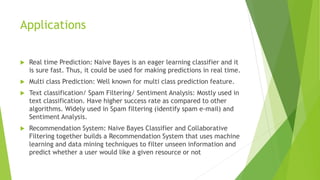
- It is commonly used for text classification like spam filtering due to its speed and accuracy.
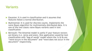
- Variants include Gaussian, Multinomial, and Bernoulli Naive Bayes for different data types.
- Limitations include its assumptions of independence and inability to tune parameters, but it remains a popular first approach for classification problems.


![Using Python
#Import Library of Gaussian Naive Bayes model
from sklearn.naive_bayes import GaussianNB
import numpy as np
#assigning predictor and target variables
X= np.array([[-3,7],[1,5], [1,2], [-2,0], [2,3], [-4,0], [-1,1], [1,1], [-2,2],
[2,7], [-4,1], [-2,7]])
y = np.array([3, 3, 3, 3, 4, 3, 3, 4, 3, 4, 4, 4])
#Create a Gaussian Classifier
model = GaussianNB()
# Train the model using the training sets
model.fit(X, y)
#Predict Output
predicted= model.predict([[1,2],[3,4]])
print(predicted)](https://image.slidesharecdn.com/naive-220827042219-07a0c734/85/Naive-pdf-9-320.jpg)